Compressed Data Structures for Binary Relations in Practice

Abstract

Binary relations are commonly used in Computer Science for modeling data. In addition to classical representations using matrices or lists, some compressed data structures have recently been proposed to represent binary relations in compact space, such as the $k^{2}$-tree and the Binary Relation Wavelet Tree (BRWT). Knowing their storage needs, supported operations and time performance is key for enabling an appropriate choice of data representation given a domain or application, its data distribution and typical operations that are computed over the data.

In this work, we present an empirical comparison among several compressed representations for binary relations. We analyze their space usage and the speed of their operations using different (synthetic and real) data distributions. We include both neighborhood and set operations, also proposing algorithms for set operations for the BRWT, which were not presented before in the literature. We conclude that there is not a clear choice that outperforms the rest, but we give some recommendations of usage of each compact representation depending on the data distribution and types of operations performed over the data. We also include a scalability study of the data representations.

=-15pt

I Introduction

Let $A$ and $B$ be two sets of objects. A binary relation $R$ is defined as a subset of the Cartesian product $A\times B$, where for each element $(a,b)\in R$, we say that $a$ is related to $b$ and denote this as $aRb$. In the areas of Mathematics and Computer Science, binary relations constitute a fundamental conceptual and methodological tool [1] used for representing properties or relationships among objects in a simple and intelligent way [2]. In Computer Science, binary relations can be modeled by using data structures such as graphs, trees, inverted indices, or discrete grids [3, 4]. By using binary relations, it is possible to model complex problems. For instance, connections among pages of a particular Web site, or even among all pages in the World Wide Web (WWW) [5, 6, 7, 8]; other fields are automated recommendation systems, where the users (customers) are related to purchased products [9, 10, 11].

For these relations we can name a number of Neighborhood queries, such as those defined in [12]. Consider a relation $R\subseteq A\times B$, with a total ordering $\leq_{A}$ in $A$ and a total ordering $\leq_{B}$ in $B$. Then, we define the following operations:

• $isRelated(x,y)=true\mbox{ if }xRy,~{}false\mbox{ otherwise}$.

• $successors(x)=\{y\in B|xRy\}$

• $predecessors(y)=\{x\in A|xRy\}$

• $rangeNeighborhood(x_{1},y_{1},x_{2},y_{2})=\{(x,y)|xRy,$ $x_{1}\leq_{A}x\leq_{A}x_{2}\wedge y_{1}\leq_{B}y\leq_{B}y_{2}\}$

Binary relations have been traditionally stored using either adjacency matrices or adjacency lists. However, and due to the growth on the size that the sets of binary relations currently generated are experiencing (for example, a graph of the whole WWW), it is convenient to store these sets using compact data structures. The goal of doing so is to reduce the storage needs (either RAM or disk), but maintaining the capacity of processing the data directly in their compressed form. Reducing the storage size may have the advantage of diminishing, even removing, the need for I/O operations.

One of the most widely known compact data structures used to store binary relations are the $k^{2}$-tree [8] and the Binary Relation Wavelet Tree (BRWT) [13], which is based on a Wavelet Tree [14]. In general, these structures support only some basic operations. For example, the $k^{2}$-tree was initially proposed to represent Web graphs, so it implemented operations such as $isRelated$ (which tests whether page $X$ links to page $Y$, called $access$ in the original paper), finding successor or predecessor neighbors, and range neighborhood queries. More recently, in [15], the operations over $k^{2}$-trees were extended to include set operations, that is, union, intersection, or difference, among others. In the case of BRWTs, there is a number of operations defined over them, such as primitive operations obtaining the labels associated to a given object, or the range of objects associated to a given label. However, no set operations are defined over BRWTs.

When deciding which compact data structure to choose for representing binary relations in the context of a given domain or application, it is very convenient to know in advance the adequacy of the available data structures, in terms of storage needs, supported operations, and time performance. The decision can also consider the frequency of each kind of operation. For example, one application might make an intensive use of union and intersection operations, but rarely searches for predecessor neighbors or performs range neighborhood queries.

In this work, we present a comparison of three compact data structures that can be used to represent binary relations: $k^{2}$-tree, $k^{2}$-tree1 and BRWT (Binary Relation Wavelet Tree). The comparison considers the same operations for all evaluated data structures. Basically, they are set operations (union, intersection, difference, and symmetric difference) and primitive neighborhood operations (isRelated, successors, predecessors, and range neighborhood queries). The goal of this comparison is to facilitate the choice of the most accurate data structure for a particular application or domain. As an additional alternative to compact data structures, we also include in our comparison the representation of the binary relations using compressed adjacency lists (using QMX and Rice-runs encoders).

Another contribution of the current work is the design and implementation of all of the algorithms needed to perform the set operations and the neighborhood queries over binary relations represented with BRWT. Like the operations we use for $k^{2}$-trees and $k^{2}$-tree1s, these algorithms operate directly over the compact data structures, without decompressing them.

The rest of this paper is organized as follows. Section II shows a review of the compact data structures considered in the comparison. Section III describes the algorithms for performing set operations over BRWTs. Section IV shows our empirical evaluation. Finally, the last section offers the overall discussion of the results and some conclusions of this work.

II Previous work

In this section, we describe the compact data structures and encoders that will be used in our comparison.

II-A $k^{2}$-tree

A $k^{2}$-tree [8] is a succinct data structure originally designed to represent Web graphs, but it is able to represent any binary relation.

A $k^{2}$-tree for a binary relation represented by a matrix of size $n\times n$ is built as follows: the root node is associated to the whole matrix, which is divided into $k^{2}$ submatrices ($k$ rows by $k$ columns). For each of these submatrices, a child is added to the root node. We store a 0 in the node if all cells in the submatrix are 0s, or a 1 if any cell contains a 1. We then proceed recursively on all children associated to a 1. The recursion stops when the algorithm processes either an individual cell or a submatrix of 0s, so the resulting tree is not balanced.

By design, $k^{2}$-trees perform very well when the matrix has a relatively low number of 1s that are clustered together, because large areas of 0s are represented by a single 0 bit in the $k^{2}$-tree. However, each 1 in the matrix can use more than one bit in the $k^{2}$-tree, so its behavior worsens if the number of 1s increases. To avoid this problem, a variation of the $k^{2}$-tree, which we denote $k^{2}$-tree1 in this work, was designed in [16]. Basically, it represents a uniform submatrix (either full of ones or zeroes) by a single 0 (with an additional bitmap to decide whether it is full of ones or zeroes) and mixed submatrices with ones and zeroes by a 1. The recursion proceeds only for these mixed areas.

Being succinct data structures, the described conceptual trees are not stored, but only the bitmaps of their nodes. Navigation operations over $k^{2}$-trees and $k^{2}$-tree1s are described in [8] and [16], respectively. Set operations for both, including the pseudocode for the algorithms as well as empirical results on their performance, are described in [15].

II-B BRWT

A Binary Relation Wavelet Tree, or BRWT [13], is a special type of wavelet tree [17] specifically designed to represent binary relations. An example of the conceptual tree built for a given binary matrix is show in Figure 1. Each node contains two bitmaps, which correspond to two submatrices: the top and bottom halves of the original matrix. A bitmap position is set to 0 if all values in this column of the submatrix are 0s (as in column 1 for the A-D bitmap in the root node) and it is set to 1 if any cell in this column has a 1 (column 2 at the same bitmap).

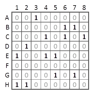
(a) A binary relation matrix

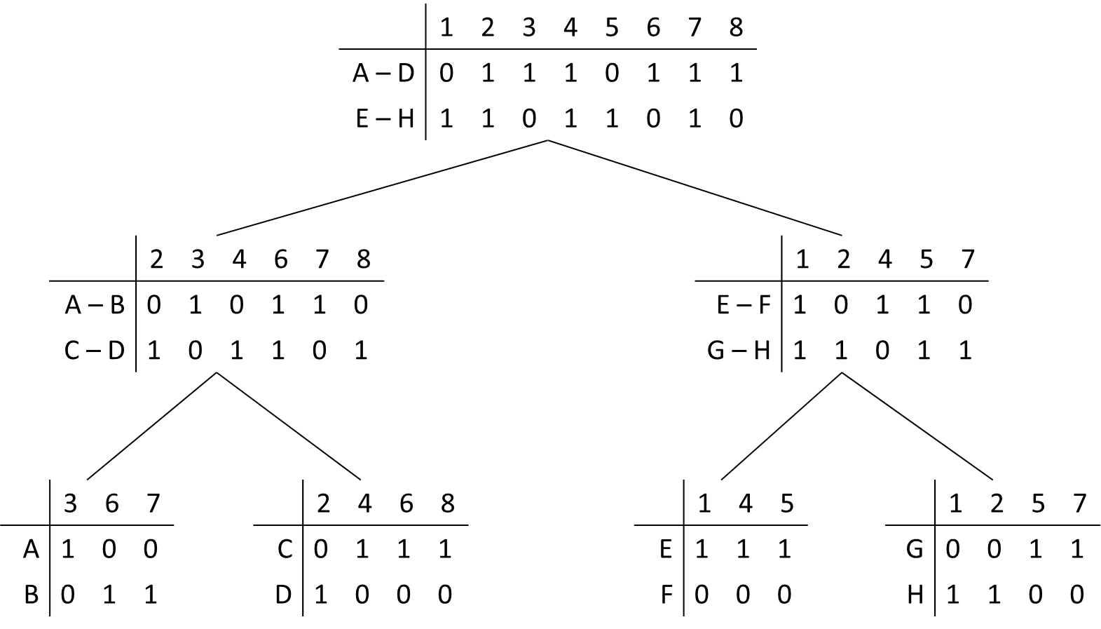
(b) Its BRWT representation

Figure 1: A BRWT example (based on [13]).

The left and right subtrees are built recursively considering the bits set to 1 at the top/bottom bitmaps. For example, column 1 does not appear in the left subtree of the root node. Note also that, like column 2, a column can propagate to both left and right subtrees. This fact makes the BRWT different from the original wavelet trees, because the bits of a given level may be more than $n$, the number of objects. Interested readers can find in [13] more information about the operations supported by BRWTs and some bounds on their complexity. We shall provide in the next section detailed information, as well as the pseudocode on which our implementation is based, of the set operations for binary relations implemented in BRWTs.

II-C Compressed adjacency lists

A very naive and (generally) space-consuming representation of a binary relation is an adjacency list. Although a valid representation, it is not suitable if the relation is big and does not fit into main memory. To avoid this problem, the adjacency lists can be compressed.

There are multiple techniques for compressing lists of integers, such as QMX and Rice-runs. QMX [18] is a compression algorithm that combines word-alignment, SIMD instructions, and run-length encoding. It also includes a SIMD-aware intersection algorithm [19]. Rice-runs combines the well-known Rice coding [20] with run-length compression [21, 22]. QMX performs really well for long adjacency lists, where SIMD instructions can be exploited. Rice-runs is specially suitable when the lists contain large sequences of consecutive 1s in the input relation matrix, due to the use of run-length compression, boosting both compression and intersection speed.

These techniques can be applied to compress any input. The authors have already used them to compress binary relations, using their own implementation in [15]. We must note, however, that these are not compact data structures. They are only compression schemes, and the lists must be decompressed before they can be used to efficiently perform the requested operations on the uncompressed data.

III Set Operations over BRWT

We now describe the algorithms for computing union, intersection, difference, and symmetric difference of binary relations represented using BRWTs.

Like the $k^{2}$-tree, BRWT is a hierarchical structure. Thus, the approach for the algorithms described in [15, 23] to implement set operations over $k^{2}$-trees can be applied here. Of course, the differences and specific properties of the BRWT must be taken into account.

The algorithms use essentially a breadth-first traversal of the trees that represent the input relations for the union, and a depth-first traversal for the remaining operations. The algorithm for the union is presented in Subsection III-A, and the algorithm for the intersection is described in Subsection  III-B. The remaining operations, difference and symmetric difference, use an algorithm very similar to the intersection, so they are briefly described in the same subsection.

For this section, given a node $b$ of the BRWT, $b_{l}$ and $b_{r}$ represent the bitmaps associated to $b$. For instance, considering $b$ the root node of the BRWT at Figure 1, $b_{l}$ is $01110111$, and $b_{r}$ is $11011010$.

III-A Breadth-first traversal algorithm (Union)

Given the properties of the union, if we are processing two nodes (of the two input BRWT), it is possible to obtain the result without accessing the children of these nodes. That is, if a bit representing a column in one of the nodes is $1$, the output is $1$ regardless of the value of the bit in the other node, and if both bits are $0$, the output is $0$. This enables the use of a breadth-first traversal over the BRWTs to compute the result of the union operation.

The traversal is performed by doing a synchronized sequential scan of the two input BRWT bitmaps $A$ and $B$. Note that this synchronization must take into account that there can exist a column that is defined in one of the two nodes being processed, but not in the other. Algorithm 1 uses queues (as usual for breadth-first traversal of any tree). In this case, each element of the queue is a pair of flags $\langle f_{A},f_{B}\rangle$ (indicating if the current column is defined in inputs $A$ and $B$, respectively), which is used to determine the output bit, and whether we should enqueue a new pair to process the current column in the child nodes (at the next level of the conceptual tree).

The algorithm actually uses two queues: $Q_{l}$ and $Q_{r}$. The reason behind their use is the way the bitmaps are stored: for each node $b$, we store the $b_{l}$ followed by the $b_{r}$. Then, $Q_{l}$ is used to manage the breadth-first traversal of the BRWT, while $Q_{r}$ is only used to process the $b_{r}$ part of each node (we can see in the algorithm that when an element is dequeued from $Q_{l}$, it is enqueued in $Q_{r}$, but the enqueuing needed to process lower levels of the conceptual tree is always done in $Q_{l}$).

Algorithm 1 UnionBRWT($A,B$)

1: $useQ_{l}\leftarrow true$

2: $pA\leftarrow 0,pB\leftarrow 0$

3: $bA\leftarrow 0,bB\leftarrow 0$

4: for $i\leftarrow 0\dots numOfObjects$ do

5:    $Q_{l}.Insert(\langle 1,1\rangle)$

6: end for

7: $Q_{l}.Insert(\langle 0,0\rangle)$

8: while $pA<|A|\vee pB<|B|$  do

9:    if $useQ_{l}$ then

10:       $\langle f_{A},f_{B}\rangle\leftarrow Q_{l}.Remove()$

11:    end if

12:    $children\leftarrow 0$

13:    while $((useQ_{l}\wedge(f_{A}\vee f_{B}))\vee(!useQ_{l}\wedge!Q_{r}IsEmpty()))$  do

14:       if $useQ_{l}$ then

15:          $Q_{r}.Insert(\langle f_{A},f_{B}\rangle)$

16:       else

17:          $\langle f_{A},f_{B}\rangle\leftarrow Q_{r}.Remove()$

18:       end if

19:       $bA\leftarrow f_{A}\wedge A[pA]$

20:       $bB\leftarrow f_{B}\wedge B[pB]$

21:       if $(bA\vee bB)\wedge(!isLeaf(pA)\vee!isLeaf(pB))$ then

22:          $Q_{l}.Insert(\langle bA,bB\rangle)$

23:          $children\leftarrow children+1$

24:       end if

25:       $R[posR]\leftarrow bA\vee bB$

26:       $posR\leftarrow posR+1$

27:       if $f_{A}$ then

28:          $pA\leftarrow pA+1$

29:       end if

30:       if $f_{B}$ then

31:          $pB\leftarrow pB+1$

32:       end if

33:       if $useQ_{l}$ then

34:          $\langle f_{A},f_{B}\rangle\leftarrow Q_{l}.Remove()$

35:       end if

36:    end while

37:    $useQ_{l}\leftarrow(\sim useQ_{l})$

38:    if $(!isLeaf(pA)\vee!isLeaf(pB))\wedge children>0$ then

39:       $Q_{l}.Insert(\langle 0,0\rangle)$

40:    end if

41: end while

42: return  $R$

III-B Depth-first traversal algorithms (intersection, difference, and symmetric difference)

The algorithms for the intersection, difference and symmetric difference use a depth-first traversal of the input BRWTs, because the output bit for a column in a node depends on the values of the same column in the descendants of this node, down to the leaves. The algorithms for the three operations are very similar, in fact the navigation scheme is exactly the same for all of them. The only changes are the value of the output, and the decision of whether it is necessary to explore the children or omit these nodes. Thus, we will explain the depth-first traversal only for the intersection, and highlight the differences for the rest of the operations.

The general idea is to process the input BRWTs column by column, recursively. Algorithm 2 describes how to perform the intersection between two BRWTs, processing every column of the root nodes calling the recursive algorithm for the intersection (Algorithm 3). An indication of how to adapt these algorithms to perform the difference and symmetric difference is shown later.

For the intersection, testing the value of a column in a given node, if both inputs have a $1$ (meaning this column is defined in both BRWTs), requires a recursive checking. However, if one of the inputs does not have this column defined, the output of the intersection will be a $0$, and there is no need to process their children. This is done for the parts $b_{l}$ and $b_{r}$ of each node $b$. For the intersection, the algorithm produces a column in the output if any of the parts ($b_{l}$ or $b_{r}$) has this column defined. Otherwise, the column is omitted in the output.

Note that, even when the access to any child could be done by using the rank and select operations for bitmaps, we considered the use of pointers to speed up the operations. The $initPointersBRWT$ operation in Algorithm 2 initializes these pointers to the start of each node. During the operation, if a column is defined in one of the BRWTs but not in the other, the $Skip$ function updates the pointers of the descendant nodes to omit this column. Otherwise, the pointers are shifted one position to process the next column after recursively computing the output value.

Algorithm 4 shows the $Skip$ function. Although in the worst case it would have to process all nodes of the BRWT, this case is extremely infrequent in practice.

Algorithm 2 IntersectBRWT($A,B$)

1: $pA\leftarrow initPointersBRWT(A)$

2: $pB\leftarrow initPointersBRWT(B)$

3: $bA\leftarrow 1,bB\leftarrow 1$

4: $idNode\leftarrow 0$

5: for $i\leftarrow 0\dots numOfObjects$ do

6:    $Intersect(A,B,pA,pB,bA,bB,R,idNode)$

7: end for

8: return  $R$

Algorithm 3 Intersect($A,B,pA,pB,rA,rB,R,idNode$)

1: $idCh_{left}\leftarrow(idNode+1)*2$

2: $idCh_{right}\leftarrow(idNode+2)*2$

3: $kl\leftarrow 0,kr\leftarrow 0$

4: $bA_{1}\leftarrow rA\wedge A[pA[idNode]]$

5: $bA_{2}\leftarrow rA\wedge A[pA[idNode+1]]$

6: $bB_{1}\leftarrow rB\wedge B[pB[idNode]]$

7: $bB_{2}\leftarrow rB\wedge B[pB[idNode+1]]$ {BEGIN code specific to Intersection}

8: if $!isLeaf(idNode)$ then

9:    if $bA_{1}\wedge bB_{1}$ then

10:       $kl\leftarrow Intersect(A,B,pA,pB,bA_{1},bB_{1},R,idCh_{left})$

11:    else if $bA_{1}$ then

12:       $Skip(A,pA,idCh_{left})$

13:    else if $bB_{1}$ then

14:       $Skip(B,pB,idCh_{left})$

15:    end if

16:    if $bA_{2}\wedge bB_{2}$ then

17:       $kr\leftarrow Intersect(A,B,pA,pB,bA_{2},bB_{2},idCh_{right})$

18:    else if $bA_{2}$ then

19:       $Skip(A,pA,idCh_{right})$

20:    else if $bB_{2}$ then

21:       $Skip(B,pB,idCh_{right})$

22:    end if

23: else

24:    $kl\leftarrow bA_{1}\wedge bB_{1}$

25:    $kr\leftarrow bA_{2}\wedge bB_{2}$

26: end if {END code specific to Intersection}

27: if $kl\vee kr\vee isRootNode(idNode)$ then

28:    $R[idNode]\leftarrow R[idNode]||kl$

29:    $R[idNode+1]\leftarrow R[idNode+1]||kr$

30: end if

31: if $rA\vee isRootNode(idNode)$ then

32:    $pA[idNode]\leftarrow pA[idNode]+1$

33:    $pA[idNode+1]\leftarrow pA[idNode+1]+1$

34: end if

35: if $rB\vee isRootNode(idNode)$ then

36:    $pB[idNode]\leftarrow pB[idNode]+1$

37:    $pB[idNode+1]\leftarrow pB[idNode+1]+1$

38: end if

39: return  $kl\vee kr$

Algorithm 4 Skip($X,pX,idNode$)

1: if $!isLeaf(idNode)$ then

2:    $bX_{1}\leftarrow X[pX[idNode]]$

3:    if $bX_{1}$ then

4:       $idCh_{left}\leftarrow(idNode+1)*2$

5:       $Skip(X,pX,idCh_{left})$

6:    end if

7:    $bX_{2}\leftarrow X[pX[idNode+1]]$

8:    if $bX_{2}$ then

9:       $idCh_{right}\leftarrow(idNode+2)*2$

10:       $Skip(X,pX,idCh_{left})$

11:    end if

12: end if

13: $pX[idNode]\leftarrow pX[idNode]+1$

14: $pX[idNode+1]\leftarrow pX[idNode+1]+1$

As Algorithm 3 shows, lines 8–26 are specific for the intersection. These lines must be modified to implement the difference and symmetric difference. The pseudocode for these changes is shown in Table I, but in summary there are basically two changes: the output bit for the column, and the management of the column when it is defined in only one BRWT. The output bit in lines 25–26 of Algorithm 3 is computed by performing the $AND$ between the two bits for the intersection, while it is the $AND$ with negated second bit for the difference, and the $EXOR$ for the symmetric difference. The recursion when the current column is defined for both input BRWTs is the same for all the algorithms, but when only one column is defined, they differ. We introduce a new $Copy$ function, which basically copies a column in one of the input bitmaps to the output bitmap. The algorithm for the difference copies the current column of the first bitmap if it is not defined in the second input. On the contrary, if the column is only defined in the second bitmap, it is skipped. For the symmetric difference, if the column is defined in either bitmap, it is copied to the output. No skipping is needed for this algorithm.

Difference

if $!isLeaf(idNode)$ then

if$bA_{1}\wedge bB_{1}$then

$kl\leftarrow RecDifference(A,B,pA,pB,bA_{1},bB_{1},R,idCh_{left})$

else if $bA_{1}$ then

$Copy(A,pA,R,idCh_{left})$

$kl\leftarrow 1$

else if $bB_{1}$ then

$Skip(B,pB,idCh_{left})$

end if      if $bA_{2}\wedge bB_{2}$ then

$kr\leftarrow RecDifference(A,B,pA,pB,bA_{2},bB_{2},idCh_{right})$

else if $bA_{2}$ then

$Copy(A,pA,R,idCh_{right})$

else if $bB_{2}$ then

$Skip(B,pB,idCh_{right})$

end if

else

$kl\leftarrow bA_{1}\wedge\sim bB_{1}$

$kr\leftarrow bA_{2}\wedge\sim bB_{2}$

end if

Symmetric difference

if $!isLeaf(idNode)$ then

if $bA_{1}\wedge bB_{1}$ then

$kl\leftarrow RecSymmDiff(A,B,pA,pB,bA_{1},bB_{1},R,idCh_{left})$

else if $bA_{1}$ then

$Copy(A,pA,R,idCh_{left})$

else if $bB_{1}$ then

$Copy(B,pB,R,idCh_{left})$

else

$kl\leftarrow 0$

end if

if $bA_{2}\wedge bB_{2}$ then

$kr\leftarrow RecSymmDiff(A,B,pA,pB,bA_{2},bB_{2},idCh_{right})$

else if $bA_{2}$ then

$Copy(A,pA,R,idCh_{right})$

else if $bB_{2}$ then

$Copy(B,pB,R,idCh_{right})$

else

$kr\leftarrow 0$

end if

else

$kl\leftarrow(\sim bA_{1}\wedge bB_{1})\vee(bA_{1}\wedge\sim bB_{1})$

$kr\leftarrow(\sim bA_{2}\wedge bB_{2})\vee(bA_{2}\wedge\sim bB_{2})$

end if

TABLE I: Code snippets for set operations.

IV Empirical Evaluation

In this section we describe the experiments we have conducted to compare the performance of the three compact data structures ($k^{2}$-trees, $k^{2}$-tree1s, and BRWT) and that of the compressed adjacency lists used to represent binary relations.

We first describe the datasets used in our experiments, of which one of them is real and three of them are synthetic. Then, we include some implementation details of our algorithms, and describe the experimental hardware and software framework we have used. Finally, we present our results.

IV-A Datasets

We ran our experiments over a real dataset (snaps-uk) and three synthetically generated distributions that use well-known random models, such as Erdős and Rényi [24], small-world (using Newman Watts-Strogatz distribution [25]), and Barabasi-Albert distribution [26]. We shall refer to these dataset distributions as random, smallworld and barabasi, respectively. Each dataset is formed by 12 files, so the metrics obtained on the sizes and timings consider the average for these files.

The snaps-uk dataset was taken from a series of twelve monthly snapshots of a Web graph from the .uk domain, collected by the Laboratory for Web Algorithmics [27, 28, 29]. We have cut down these graphs to use 1 million nodes ($n=1,000,000$). More information on this dataset is also available in [15].

The three synthetic datasets were generated using the NetworkX Python library. For the random distribution, only the number of nodes $n$ and number of edges $m$ were required as arguments. For the Barabasi-Albert and small-world distributions, a third parameter $k$ is needed, to specify the $k$-nearest neighbors to connect to a given node. This parameter determines the number of edges that is generated. If the number of generated edges is greater than the specified number $m$, the remaining edges are removed.

The output is a binary file containing the plain adjacency list, which in turn is used to build the compact data structure representations (for $k^{2}$-trees, $k^{2}$-tree1s, and BRWT) as well as the compressed adjacency lists (QMX and Rice-runs).

We have also generated 12 files for each distribution. All of them have $n=1,000,000$ nodes. In order to have the same density, the number of generated edges for each file was the same as the corresponding file for the snaps-uk dataset. That resulted in an average number of edges of $m=2,240,877$ per distribution, which gives a density $m/n^{2}=0.000224\%$.

Given that the distribution of 1s has a high impact on the size of the compressed structures, as well as in the performance of data structures, a sample of all datasets is shown in Figure 2. As we can see, the synthetically generated datasets are much less clustered than snaps-uk, the real dataset.

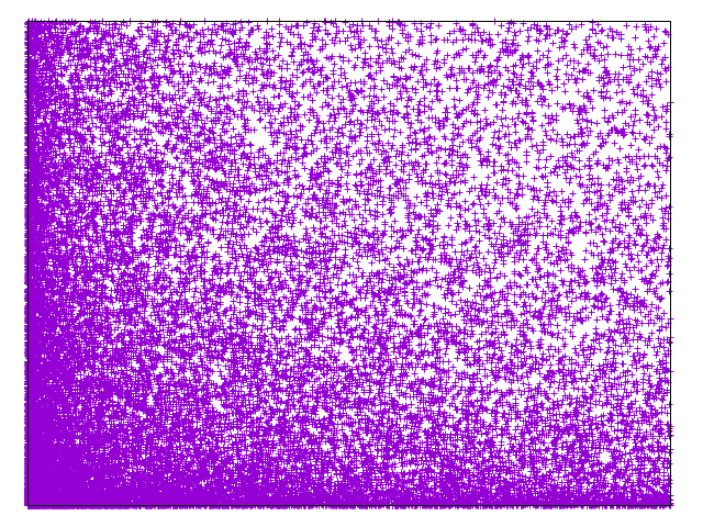
(a) Barabasi

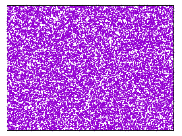
(b) random

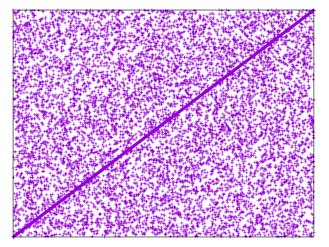
(c) smallworld

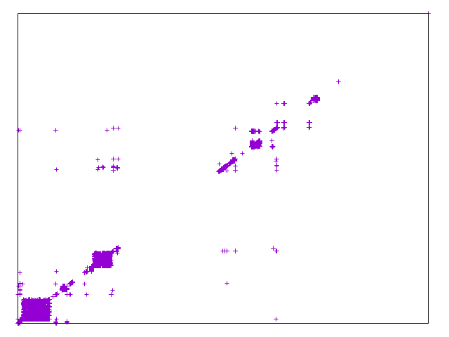
(d) snaps-uk

Figure 2: A sample of all dataset distributions.

IV-B Experimental framework

The comparison we performed considered, for all the data structures, the following operations:

• Neighborhood queries: isRelated, successors, predecessors, and range neighborhood.

• Set operations: union, intersection, difference, and symmetric difference.

The work described here required the coding of all of the algorithms (both neighborhood and set operations) for BRWT, as well as the neighborhood operations for $k^{2}$-tree1s and compressed adjacency lists using QMX and Rice-runs. For the remaining algorithms, we use the source code by the authors of the works described in [8] and [16].

The implementation language for all algorithms is C, compiled with gcc version 6.3.0. The experiments were run on an isolated Intel^® Xeon^® ES2470@2.30GHz processor with 20 MB of cache, and 64 GB of RAM. It runs Debian 10.1 (buster) with kernel 4.19.0 (64 bits).

IV-C Results

We present in this section the results of our empirical evaluation. First, we study independently the storage needs (the actual size) of the data structures, and their performance for both neighborhood queries and set operations. Then, both sizes and times are considered together in order to present some trade-offs that would apply when choosing a specific data structure. Finally, we analyze the data structures in terms of scalability.

In the neighborhood operations, besides the isRelated operation, we have included a similar one: isRelated-True. In fact, it is the same operation, but the result of the query is known to be $true$ (which corresponds to having a 1 in the matrix). Thus, isRelated-True acts as a worst-case scenario for the isRelated operation in most cases. For example, for $k^{2}$-trees, we know that this operation must navigate the tree until its leaves (the result is 1, so it cannot be discarded by a 0 in a previous level of the tree).

Also note that, for the naming of the data structures in the tables and graphics of this section, we have chosen shorter names: kt for $k^{2}$-tree, ktone for $k^{2}$-tree1, brwt for BWRT, qmx for the QMX encoder, and rice for the Rice-runs encoder.

IV-C1 Storage

The average size taken up by each structure for all distribution is shown in Table II. As a reference, the size of the full uncompressed adjacency lists is also included in the table. Our standard implementation uses 32-bit integers, so it is used as the base number. However, in order to represent a relation for 1 million nodes, only 20 bits suffice. Thus, we also show the size theoretically needed to represent this relation. Table III shows the same information as a ratio, considering the full adjacency lists as the base for comparison (value $1.0$), so the deviations can be better seen.

	barabasi	random	smallworld	snaps-uk
Full adj. list (32 bits)	12,963,523	12,963,523	12,963,523	12,963,523
Full adj. list (20 bits)	8,102,201	8,102,201	8,102,201	8,102,201
brwt	10,367,083	10,894,448	7,413,171	2,371,233
kt	9,737,915	10,724,430	4,770,940	1,419,065
ktone	15,613,223	17,304,302	7,344,613	1,771,421
qmx	16,567,964	22,101,395	19,599,142	7,569,547
rice	13,808,180	17,651,437	14,440,775	6,672,224

TABLE II: Average size (in bytes) for the different datasets.

	barabasi	random	smallworld	snaps-uk
Full adj. list (32 bits)	1.00	1.00	1.00	1.00
Full adj. list (20 bits)	0.63	0.63	0.63	0.63
brwt	0.80	0.84	0.57	0.18
kt	0.75	0.83	0.37	0.11
ktone	1.20	1.33	0.57	0.14
qmx	1.28	1.70	1.51	0.58
rice	1.07	1.36	1.11	0.51

TABLE III: Average size, shown as a ratio.

Considering the datasets, we can see that the distribution that allows for the best compression ratios (actually, the only one that gets compressed by all structures) is snaps-uk. This is reasonable, because this distribution is clustered, unlike the three synthetic ones, which are based on random models. More concretely, the best compression ratios are obtained by the $k^{2}$-tree variants, which benefit from distributions of small number of ones that are clustered. As for the QMX and Rice-runs, their behavior is worse, because they are based on run-length compression, and having a smaller runs of 1s produces worse compression ratios.

Considering the compressed data structures, we can see that standard $k^{2}$-trees obtain better results than the plain adjacency list using 20 bits for those clustered distributions (smallworld and snaps-uk), but not for those that follow a more random model (barabasi and random). In any case, compressed data structures obtain generally better results than compressed adjacency lists (except in the case of barabasi, which obtains better results for Rice-runs than for $k^{2}$-tree1). Compressed adjacency lists require, for all synthetic data distributions, larger spaces than the original plain representation. For example, using QMX to compress the random distribution actually obtains a file 70% bigger than the full adjacency lists using 32 bits.

IV-C2 Timings

The timings shown in this section consider only the time devoted to the operations themselves, without taking into account the I/O time of reading the structures (for neighborhood and set operations) or writing the result (only for set operations). In the case of the neighborhood operations, the time shown corresponds to the execution of $1,000$ queries of the same type over the same structure.

Let us first discuss the neighborhood operations. Their timings, in milliseconds, are shown in Table IV. For a better comparison, Table V shows the same information as ratios. The value $1.00$ corresponds to the shortest time for the operation on a distribution.

Query		barabasi	random	smallworld	snaps-uk
isRelated	brwt	0.312	0.418	0.261	0.075
	kt	0.975	1.240	1.057	0.313
	ktone	0.867	1.192	1.122	0.453
	qmx	0.565	0.941	0.602	0.162
	rice	0.460	0.586	0.456	0.135
isRelated-True	brwt	4.539	4.563	4.607	6.103
	kt	2.768	2.601	2.620	3.318
	ktone	2.899	3.501	2.506	3.260
	qmx	1.461	1.121	1.103	3.690
	rice	1.335	0.655	0.645	3.023
predecessors	brwt	19.814	20.709	16.269	14.018
	kt	270.140	356.439	190.632	11.515
	ktone	444.631	653.985	304.679	14.634
	qmx	337111.835	468610.372	358252.193	101397.174
	rice	206217.818	270400.268	200732.389	78405.505
successors	brwt	16.258	18.792	16.278	16.322
	kt	263.515	334.947	189.781	10.459
	ktone	437.586	635.259	298.441	13.610
	qmx	0.660	0.841	0.755	0.269
	rice	0.461	0.641	0.482	0.195
rangeNeighborhood	brwt	35.709	40.745	32.419	21.644
	kt	1.767	2.461	1.371	0.316
	ktone	4.308	6.175	1.860	0.373
	qmx	80.690	110.513	124.586	53.651
	rice	75.017	88.380	76.048	48.724

TABLE IV: Timings for neighborhood queries (in ms).

Query		barabasi	random	smallworld	snaps-uk
isRelated	brwt	1.00	1.00	1.00	1.00
	kt	3.13	2.97	4.05	4.17
	ktone	2.78	2.85	4.30	6.04
	qmx	1.81	2.25	2.31	2.16
	rice	1.47	1.40	1.75	1.80
isRelated-True	brwt	3.40	6.97	7.14	2.02
	kt	2.07	3.97	4.06	1.10
	ktone	2.17	5.35	3.89	1.08
	qmx	1.09	1.71	1.71	1.22
	rice	1.00	1.00	1.00	1.00
predecessors	brwt	1.00	1.00	1.00	1.22
	kt	13.63	17.21	11.72	1.00
	ktone	22.44	31.58	18.73	1.27
	qmx	17013.82	22628.34	22020.54	8805.66
	rice	10407.68	13057.14	12338.34	6808.99
successors	brwt	35.27	29.32	33.77	83.70
	kt	571.62	522.54	393.74	53.64
	ktone	949.21	991.04	619.17	69.79
	qmx	1.43	1.31	1.57	1.38
	rice	1.00	1.00	1.00	1.00
rangeNeighborhood	brwt	20.21	16.56	23.65	68.49
	kt	1.00	1.00	1.00	1.00
	ktone	2.44	2.51	1.36	1.18
	qmx	45.66	44.91	90.87	169.78
	rice	42.45	35.91	55.47	154.19

TABLE V: Timings for neighborhood queries (ratio).

The information that stands out most in these tables corresponds to the predecessors operation, where the fastest structure is the BRWT, and the QMX and Rice-runs encoders are much slower (up to $22,628$ times slower in the case of the random dataset). This is reasonable because encoders compress the adjacency lists row by row, and finding the predecessors requires the decompression of all of the encoded lists.

For successors, however, Rice-runs is the fastest, closely followed by QMX, while $k^{2}$-trees and $k^{2}$-tree1s are slower (almost $1,000$ times). The reason is that, in this case, the encoders have to decompress only one list (at most; if there are no 1s in the row, the answer is immediate).

Considering together predecessors and successors, we can see that the difference between the best and the worst is much larger in the predecessors because, as we mentioned, QMX and Rice-runs must decode all of the lists. However, for successors, the compact data structures have to explore only part of the binary relation, not all of it. This is because all of them are actually self-indices, so they allow for a fast access to a portion of the matrix. For the same reason, if we consider the rangeNeighborhood queries, we can see that the compact data structures perform better than the encoders, and, in this case, $k^{2}$-tree is the fastest structure.

For the isRelated and isRelated-True queries, all structures offer a more homogeneous behavior. Anyway, BRWT is the fastest for isRelated, while it is Rice-runs for isRelated-True. This is due to the fact that isRelated accesses a random cell in the matrix, and with a low density BRWT is able to answer false without reaching the leaf nodes, while in the case of isRelated-True query, BRWT must always reach a leaf node. The same happens for $k^{2}$-trees and $k^{2}$-tree1s.

Operation		barabasi	random	smallworld	snaps-uk
Difference	brwt	8228.666	9336.838	3706.757	745.321
	kt	4244.713	5001.098	1942.896	349.290
	ktone	5468.160	6072.274	2188.450	265.957
	qmx	715.745	890.225	694.532	310.097
	rice	480.035	563.134	377.019	148.794
Intersection	brwt	3887.119	4313.796	2304.365	610.479
	kt	2543.189	3095.668	1233.486	199.862
	ktone	4958.742	5491.372	2040.778	224.208
	qmx	562.268	682.922	680.239	321.681
	rice	284.395	335.176	367.698	153.825
Symmetric	brwt	11817.572	17987.314	5173.330	767.283
Difference	kt	5778.197	6716.642	2676.058	527.112
	ktone	5317.761	6253.623	2385.553	379.348
	qmx	819.924	952.049	724.674	346.717
	rice	561.967	661.309	445.186	126.816
Union	brwt	7371.075	7960.348	4201.526	1218.818
	kt	4117.581	4517.057	1927.165	571.612
	ktone	5552.810	6351.123	2392.387	444.056
	qmx	841.915	999.932	780.056	410.269
	rice	624.011	680.933	524.918	271.250

TABLE VI: Timings for set operations (in ms).

Operation		barabasi	random	smallworld	snaps-uk
Difference	brwt	17.14	16.58	9.83	5.01
	kt	8.84	8.88	5.15	2.35
	ktone	11.39	10.78	5.80	1.79
	qmx	1.49	1.58	1.84	2.08
	rice	1.00	1.00	1.00	1.00
Intersection	brwt	13.67	12.87	6.27	3.97
	kt	8.94	9.24	3.35	1.30
	ktone	17.44	16.38	5.55	1.46
	qmx	1.98	2.04	1.85	2.09
	rice	1.00	1.00	1.00	1.00
Symmetric	brwt	21.03	27.20	11.62	6.05
Difference	kt	10.28	10.16	6.01	4.16
	ktone	9.46	9.46	5.36	2.99
	qmx	1.46	1.44	1.63	2.73
	rice	1.00	1.00	1.00	1.00
Union	brwt	11.81	11.69	8.00	4.49
	kt	6.60	6.63	3.67	2.11
	ktone	8.90	9.33	4.56	1.64
	qmx	1.35	1.47	1.49	1.51
	rice	1.00	1.00	1.00	1.00

TABLE VII: Timings for set operations (ratio).

For the set operations, Table VI shows the actual times of our experiments, and the same information as ratios is shown in Table VII. Even when the difference between the best and worst data structure is not as large as for neighborhood operations, it is clear that the encoders (Rice-runs, closely followed by QMX) are the best option. The BRWT is almost always the slowest for these kinds of operations.

The reason behind that behavior is that set operations must access in general all the elements of the binary relation. The encoders just decompress row by row, build the result and encode it as a new output row. However, the three compact data structures, being self-indices, have an overhead that (as in general for any type of index) worsens the performance when the full dataset has to be accessed.

IV-C3 Storage size versus time

Let us consider now the trade-off between storage size and performance for all compared data structures. Figures 3–7 analyze their behavior. All figures contain two graphics: $(a)$ for the neighborhood operations, and $(b)$ for the set operations.

For the neighborhood operations, it is clear that the compact data structures, especially the standard $k^{2}$-tree, is the best option, in terms of both size and performance, while the encoders use more space and perform worse. Figure 3 shows this behavior considering an average of all the datasets together. If we take into account the data distribution, we can see that the previous conclusion is generally true, except for the $k^{2}$-tree1. This data structure is highly dependant on the degree of clustering (remember that it compresses areas of 1s in the matrix), and thus its size grows for non-clustered datasets (like barabasi, and random, as seen in Figures 4 and 5 respectively), and it behaves better for the more clustered (smallworld and and especially snaps-uk, as seen in Figures 6 and 7 respectively).

For the set operations, none of the data structures outperforms the rest in terms of size and performance. On the contrary, we can see in Figure 3 that we have a trade-off, because the compact data structures use less space, but they are slower than the encoders. The encoders are faster, but they need more space. Thus, the general advice would be the following: if we are primarily interested in speed, and there is enough available RAM to fit the data structures using the encoders, then use the encoders. If the datasets would not fit into RAM, use the compact data structures.

Parts $(b)$ of Figures 4–7 show this behavior for each data distribution. We can see that the BRWT is a poor choice for the set operations in any distribution in terms of speed (not in terms of space). Again, the $k^{2}$-tree1 shows a behavior highly dependent on the clusterization, being one of the fastest data structures for the snaps-uk dataset and one of the slowest technique for barabasi.

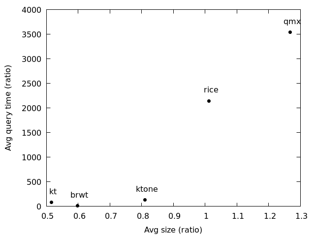
(a) Neighborhood operations

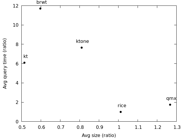
(b) Set operations

Figure 3: Average time versus average size for all distributions.

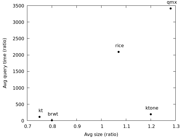
(a) Neighborhood operations

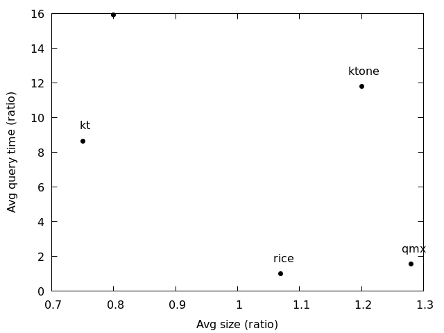
(b) Set operations

Figure 4: Average time versus average size for barabasi.

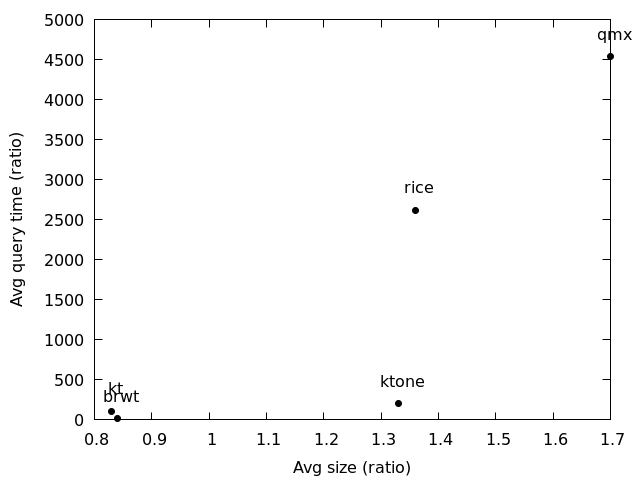
(a) Neighborhood operations

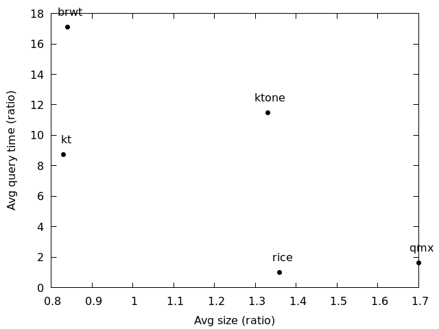
(b) Set operations

Figure 5: Average time versus average size for random.

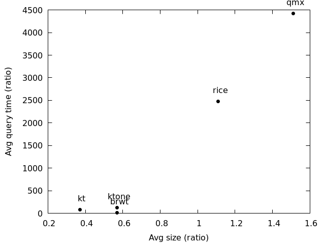
(a) Neighborhood operations

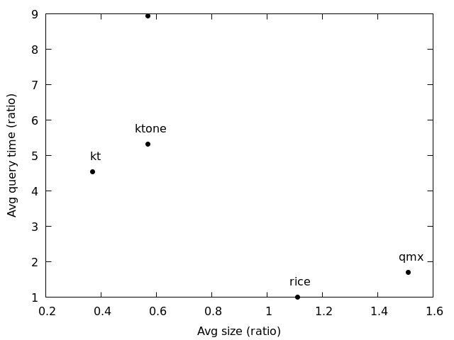
(b) Set operations

Figure 6: Average time versus average size for smallworld.

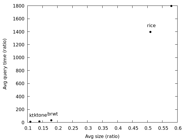
(a) Neighborhood operations

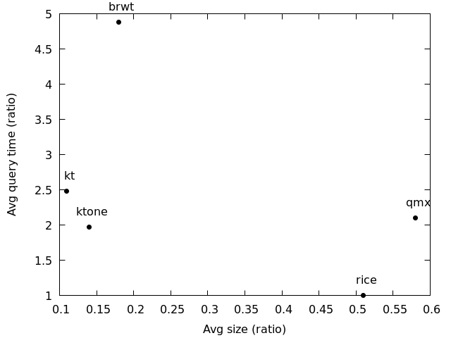
(b) Set operations

Figure 7: Average time versus average size for snaps-uk.

IV-D A note on scalability

The previous section analyzed the performance of the data structures over relations having 1 million nodes. However, we are also interested in the behavior of the data structures when the size of the relation grows.

We shall describe in this section the behavior of the data structures when the number of nodes varies, growing up to $10,000,000$ nodes. We have chosen the smallworld data distribution for these experiments, because it is the less biased distribution: it is not as clustered as the real dataset (snaps-uk), which would benefit the compact data structures, and it is not as evenly distributed as random or barabasi, which would benefit the QMX and Rice-runs encoders. The dataset was generated also using the NetworkX Python library, considering a value of 2 for the $k$ parameter (indicating the $k$ nearest neighbors that would be linked in the graph) in all cases.

Let us first analyze the neighborhood operations shown in Figure 8. In general, we can see that the data structures behavior is as expected from the previous analysis. The encoders scale very well for the isRelated-True and successors operations. Note that we have chosen the isRelated-True operation instead of isRelated, in order to force the structures to either navigate down the tree (compact data structures) or decompress a non-empty list (for the encoders). We also concluded that the encoders performed badly for predecessors, and this gets confirmed here. In fact, this operation could not be completed for the relations with 5 and 10 million nodes, with our hardware configuration. If we remove the encoders from the plot (Figure 8(d)), we can see that the BRWT scales well (almost constant) while the remaining compact data structures scale in a logarithmic order. It is also worth noticing that the $k^{2}$-tree and $k^{2}$-tree1 have a similar trend in all operations.

For the rangeNeighborhood operation, shown in Figure 9, we have tested the scalability in two different ways: varying the number of nodes (as in the previous cases) but maintaining a fixed range size of $500\times 500$, and fixing the number of nodes but varying the range size (up to $50,000\times 50,000$). It might seem strange that QMX and Rice-runs solve the range queries faster when the number of nodes increases. However, this can be explained, as when the number of nodes increases, the number of empty rows will probably increase too. Therefore, the number of rows actually explored and decompressed decreases, so the time to solve the query is shorter. Note that the behavior of the compact data structures is quite similar (it is not decreasing, but almost constant). Considering the variation of the range size, we can see that all data structures increase the time for longer ranges, but in a sublinear order in general, being the $k^{2}$-tree and $k^{2}$-tree1 the most efficient data structures.

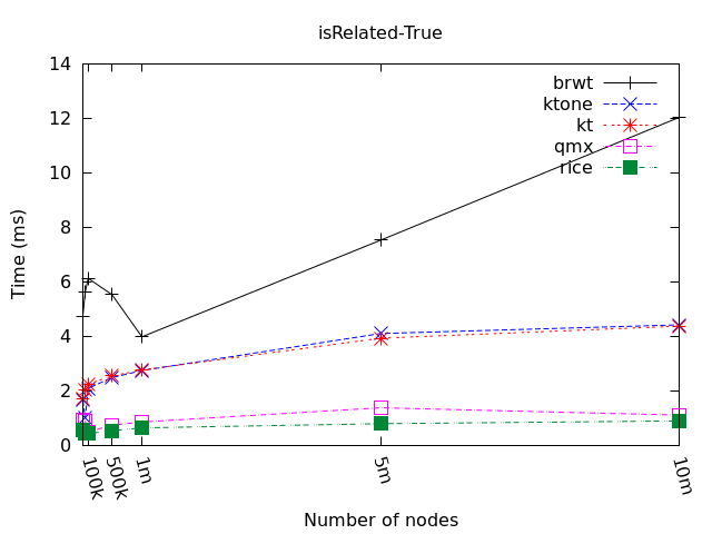
(a) isRelated

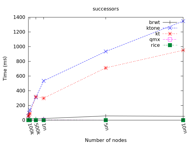
(b) successors

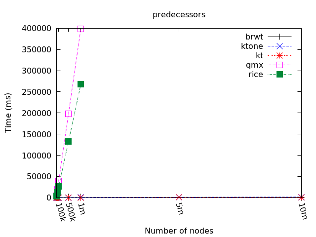
(c) predecessors

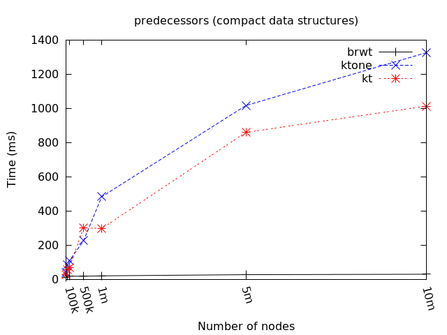
(d) predecessors (compact)

Figure 8: Number of nodes versus average time on neighborhood operations for scalability.

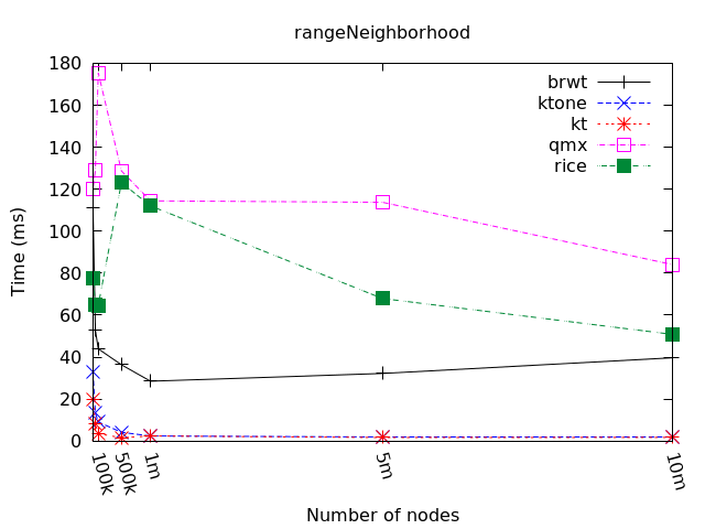
(a) Varying the number of nodes

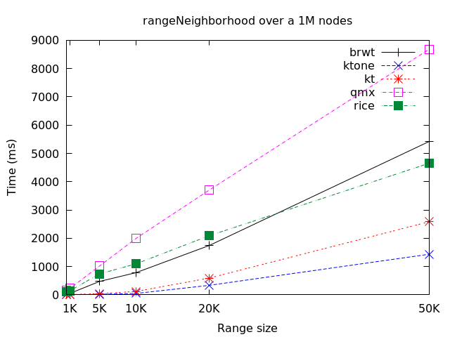
(b) Varying the range size

Figure 9: Scalability measures for rangeNeighborhood queries

For the set operations, illustrated in Figure 10, all data structures scale quite well, and in a uniform way (note that there are no crosses among the lines in the figure). We can highlight that the BRWT is the worst option for these operations, while the encoders are the more suitable ones. This confirms what was shown in Section IV-C2.

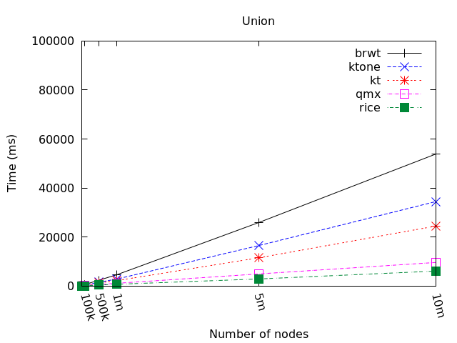
(a) Union

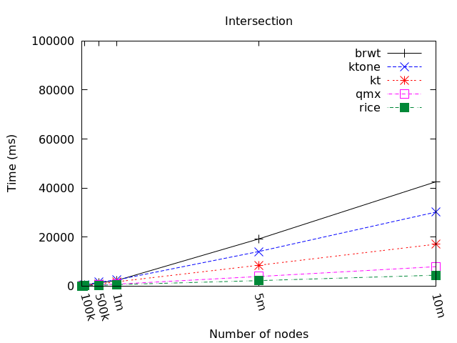
(b) Intersection

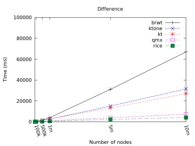
(c) Difference

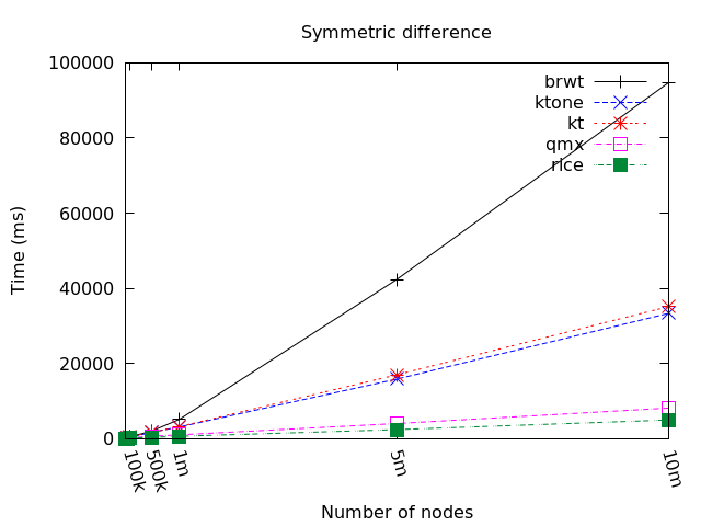
(d) Symmetric Difference

Figure 10: Number of nodes versus average time on set operations for scalability.

A final note about scalability, but regarding some implementation decisions for our algorithms: as we mentioned in Section III-B, we decided to use a set of pointers instead of using the rank and select operations to speed up the depth-first set operations over BRWTs. The same decision was taken to speed up the operations over both variants of $k^{2}$-trees. Figure 11 shows the behavior of the intersection algorithm using both implementations. The version with pointers clearly outperforms the rank/select version, especially for large datasets (up to 3 times faster). Of course, this speed-up comes with a price, because the pointer version takes up more memory (between 30% and 56%).

Figure 11: Speed improvement of queries on BRWT by using pointers

V Conclusions

In this work, we have conducted several experiments to compare the behavior of several data structures used to store binary relations. We have considered three compact data structures ($k^{2}$-tree, $k^{2}$-tree1 and BRWT) and two encoders or compressors (QMX and Rice-runs).

For the compact data structures, we used the algorithms for $k^{2}$-trees and $k^{2}$-tree1s developed in [8] and [15], but the algorithms for set operation over the BRWT are presented here for the first time, thus extending the functionality of this data structure.

We have found that there is no clear winner, no data structure is better than the rest in all cases. All of them have some advantages and disadvantages, depending on several factors. We have considered the storage size and the response time as basic measurements, and have tested them using several datasets with different characteristics, because the data distribution has a great impact on the performance of all data structures.

In order to offer some general conclusions, we can group the data structures in three groups that have a similar behavior: the encoders (QMX and Rice-runs), both $k^{2}$-tree variants, and BRWT.

With respect to the encoders, they proved to be the fastest option for the set operations in all cases, and are competitive for some neighborhood queries, except for rangeNeighborhood and especially the predecessors queries (which could not actually be executed for large datasets). In terms of storage needs, the encoders use in general more space than the compact data structures.

The $k^{2}$-trees excel at the rangeNeighborhood queries, but are outperformed for the successors operation. For the rest of the neighborhood queries they are competitive. For the set operations, these structures are not as fast as the encoders, but they are the best option amongst the compact data structures. They also scale reasonably well when the dataset grows. In terms of storage, $k^{2}$-trees are always the best option, using much less space than the other structures. This can let the $k^{2}$-tree be a good option for those operations where they are slower than the encoders, when the encoders cannot fit the relation into main memory.

BRWT is competitive for the neighborhood queries in general, and is the best option for the predecessors queries. For the set operations, however, it is usually the worst option. In terms of storage needs, it is competitive with respect to the remaining compact data structures, and better than the encoders.

Finally, we must highlight that the data distribution has a great impact on both the size of the data structure and the speed of the operations. In general, clustered data distributions tend to favor compact data structures, while more random or evenly distributed datasets tend to benefit the encoders.

We have presented here, to the best of our knowledge, the first study about the behavior of compressed data structures for binary relations, evaluating storage needs and speed of the operations based on different (synthetic and real) data distributions, considering also the scalability of the data structures.

Carlos Quijada Fuentes obtained his degree in Civil Engineering in Computer Science in 2011 and his Master in Computer Science in 2017, both from the University of Bío-Bío. His research area is data structures and algorithms. Chillán/Chile.

Miguel R. Penabad obtained his Master in Computer Science in 1994 at the University of A Coruña. He received his Ph.D in 2001 at the University of A Coruña. He is a professor in the same university since 2000. His main research interests are database query optimization, and algorithms and data structures for information retrieval.

Susana Ladra received the bachelor’s degree in mathematics from the National Distance Education University (UNED), in 2014, and the master’s in computer science engineering and the Ph.D. degree in computer science from the University of A Coruña, in 2007 and 2011, respectively. She is currently an Associate Professor with the Universidade da Coruña. She is the Principal Investigator of several national and international research projects. She has published more than 40 articles in various international journals and conferences. Her research interests include design and analysis of algorithms and data structures, and data compression and data mining in the fields of information retrieval and bioinformatics.

Gilberto Gutiérrez Retamal received his M. Sc. from the University of Chile in 1999 and the Ph.D. in computer science in 2007 from the same university. His research areas include data structures and algorithms, spatial and spatio-temporal databases. He is currently an associate professor in the Department of Computer Science and Information Technology, at the University of Bío-Bío, Chillán / Chile.

References

- [1] D. J. Dougherty and C. Gutiérrez, “Normal forms for binary relations,” Theoretical Computer Science, vol. 360, no. 1, pp. 228 – 246, 2006. [Online]. Available: http://www.sciencedirect.com/science/article/pii/S0304397506002787
- [2] J. Ah-Pine, “A general framework for comparing heterogeneous binary relations,” in Geometric Science of Information, F. Nielsen and F. Barbaresco, Eds. Berlin, Heidelberg: Springer Berlin Heidelberg, 2013, pp. 188–195.
- [3] N. R. Brisaboa, G. de Bernardo, and G. Navarro, “Compressed dynamic binary relations,” in Procs. of DCC, 2012, pp. 52–61.
- [4] N. Brisaboa, A. Cerdeira-Pena, G. de Bernardo, and G. Navarro, “Compressed representation of dynamic binary relations with applications,” Information Systems, vol. 69, pp. 106–123, 2017.
- [5] A. Broder, R. Kumar, F. Maghoul, P. Raghavan, S. Rajagopalan, R. Stata, A. Tomkins, and J. Wiener, “Graph structure in the web,” Comput. Netw., vol. 33, no. 1-6, pp. 309–320, Jun. 2000. [Online]. Available: http://dx.doi.org/10.1016/S1389-1286(00)00083-9
- [6] P. Boldi and S. Vigna, “The webgraph framework i: Compression techniques,” in Proceedings of the 13th International Conference on World Wide Web, ser. WWW ’04. New York, NY, USA: ACM, 2004, pp. 595–602. [Online]. Available: http://doi.acm.org/10.1145/988672.988752
- [7] P. Papadimitriou, A. Dasdan, and H. Garcia-Molina, “Web graph similarity for anomaly detection,” Journal of Internet Services and Applications, vol. 1, no. 1, pp. 19–30, May 2010. [Online]. Available: https://doi.org/10.1007/s13174-010-0003-x
- [8] N. R. Brisaboa, S. Ladra, and G. Navarro, “Compact representation of web graphs with extended functionality,” Information Systems, vol. 39(1), pp. 152–174, 2014.
- [9] B. Awerbuch, B. Patt-Shamir, D. Peleg, and M. Tuttle, “Improved recommendation systems,” in Proceedings of the Sixteenth Annual ACM-SIAM Symposium on Discrete Algorithms, ser. SODA ’05. Philadelphia, PA, USA: Society for Industrial and Applied Mathematics, 2005, pp. 1174–1183. [Online]. Available: http://dl.acm.org/citation.cfm?id=1070432.1070599
- [10] Z. Heng-Ru, M. Fan, and X. Yuan-Yuan, “A hybrid recommender system based on user-recommender interaction,” Mathematical Problems in Engineering, vol. 2015, p. 11, 2015.
- [11] G. Navarro, Compact Data Structures – A practical approach. Cambridge University Press, 2016, iSBN 978-1-107-15238-0. 536 pages.
- [12] Y. Yao, “Semantics of fuzzy sets in rough set theory,” in Transactions on rough sets II. Springer, 2004, pp. 297–318.
- [13] J. Barbay, F. Claude, and G. Navarro, “Compact binary relation representations with rich functionality,” Infomation and Computation, vol. 232, pp. 19–37, 2013.
- [14] R. Grossi, A. Gupta, and J. S. Vitter, “High-order entropy-compressed text indexes,” in Proceedings of the Fourteenth Annual ACM-SIAM Symposium on Discrete Algorithms, ser. SODA ’03. Philadelphia, PA, USA: Society for Industrial and Applied Mathematics, 2003, pp. 841–850. [Online]. Available: http://dl.acm.org/citation.cfm?id=644108.644250
- [15] C. Quijada-Fuentes, M. R. Penabad, S. Ladra, and G. Gutiérrez, “Set operations over compressed binary relations,” Information Systems, vol. 80, pp. 76 – 90, 2019. [Online]. Available: http://www.sciencedirect.com/science/article/pii/S0306437917302612
- [16] G. de Bernardo, S. Álvarez-García, N. R. Brisaboa, G. Navarro, and O. Pedreira, “Compact querieable representations of raster data,” in Procs. of SPIRE, 2013, pp. 96–108.
- [17] R. Grossi, A. Gupta, and J. Vitter, “High-order entropy-compressed text indexes,” Proceedings of the Annual ACM-SIAM Symposium on Discrete Algorithms, pp. 841–850, 2003.
- [18] A. Trotman, “Compression, SIMD, and postings lists.” in Proc. 19th Australasian Document Computing Symposium (ADCS), 2014, pp. 50–57.
- [19] D. Lemire, L. Boytsov, and N. Kurz, “SIMD compression and the intersection of sorted integers,” Software: Practice and Experience, vol. 46(6), pp. 723–749, 2016.
- [20] I. Witten, A. Moffat, and T. Bell, Managing Gigabytes. Morgan Kaufmann, 2nd edition, 1999.
- [21] J. Culpepper and A. Moffat, “Efficient set intersection for inverted indexing,” ACM Transactions on Information Systems), vol. 29, no. 1, p. art. 1, 2010.
- [22] F. Transier and P. Sanders, “Engineering basic algorithms of an in-memory text search engine,” ACM Transactions on Information Systems), vol. 29, no. 1, p. art. 2, 2010.
- [23] N. R. Brisaboa, G. de Bernardo, G. Gutiérrez, S. Ladra, M. R. Penabad, and B. A. Troncoso, “Efficient set operations over k2-trees,” in 2015 Data Compression Conference, DCC 2015, Snowbird, UT, USA, April 7-9, 2015. IEEE, 2015, pp. 373–382. [Online]. Available: https://doi.org/10.1109/DCC.2015.9
- [24] P. Erdős and A. Rényi, “On random graphs i.” Publicationes Mathematicae (Debrecen), vol. 6, pp. 290–297, 1959 1959.
- [25] M. Newman, S. Strogatz, and D. Watts, “Random graphs with arbitrary degree distributions and their applications,” Arxiv preprint cond-mat/0007235, 2001.
- [26] R. Albert and A.-L. Barabási, “Statistical mechanics of complex networks,” Reviews of Modern Physics, vol. 74, pp. 47–97, Jan. 2002.
- [27] P. Boldi and S. Vigna, “The WebGraph framework I: Compression techniques,” in Proc. of the Thirteenth International World Wide Web Conference (WWW 2004). Manhattan, USA: ACM Press, 2004, pp. 595–601.
- [28] P. Boldi, M. Rosa, M. Santini, and S. Vigna, “Layered label propagation: A multiresolution coordinate-free ordering for compressing social networks,” in Proceedings of the 20th international conference on World Wide Web, S. Srinivasan, K. Ramamritham, A. Kumar, M. P. Ravindra, E. Bertino, and R. Kumar, Eds. ACM Press, 2011, pp. 587–596.
- [29] P. Boldi, M. Santini, and S. Vigna, “A large time-aware graph,” SIGIR Forum, vol. 42, no. 2, pp. 33–38, 2008.