We compute the exact partition function of the isotropic 6-vertex model on a cylinder geometry with free boundary conditions, for lattices of intermediate size, using Bethe ansatz and algebraic geometry. We perform the computations in both the open and closed channels. We also consider the partial thermodynamic limits, whereby in the open (closed) channel, the open (closed) direction is kept small while the other direction becomes large. We compute the zeros of the partition function in the two partial thermodynamic limits, and compare with the condensation curves.

1 Introduction

Computing partition functions of integrable vertex models at intermediate lattice size is a hard problem. For small lattice size, the partition function can be computed simply by brute force. For large lattice size, where the thermodynamic limit is a good approximation, various methods are available, including the Wiener-Hopf method [1, 2, 3], non-linear integral equations [4, 5] and a distribution approach [6]. At intermediate lattice size, brute force is no longer an option, and the thermodynamic approximation is inaccurate. In a previous work [7], three of the authors developed an efficient method to compute the exact partition function of the 6-vertex model analytically for intermediate lattice size. They considered the 6-vertex model at the isotropic point on the torus, i.e. with periodic boundary conditions in both directions. The method is based on the rational $Q$-system [8] and computational algebraic geometry (AG). The algebro-geometric approach to Bethe ansatz was initiated in [9], with the general goal of exploring the structure of the solution space of Bethe ansatz equations (BAE) and developing new methods to obtain analytic results in integrable models. The simplest example for such a purpose is the BAE of the $SU(2)$-invariant Heisenberg XXX spin chain with periodic boundary conditions. It is an interesting question to generalize these methods to more sophisticated cases such as higher-rank spin chains, quantum deformations and non-trivial boundary conditions.

In the current work, we take one step forward in this direction and consider the partition function of the 6-vertex model on the cylinder. Namely, we take one direction of the lattice to be periodic and impose free open boundary conditions in the other direction. This set-up has several new features compared to the torus geometry already considered in [7].

First of all, to consider open boundary conditions for the vertex model, we put the model on a diagonal square lattice where each square is rotated by $45^{\circ}$, as is shown in figure 2.1. The partition function on such a lattice can be formulated in terms of a diagonal-to-diagonal transfer matrix [10], which does not commute for different values of the spectral parameter. Nevertheless, the $R$-matrix approach (the so-called Quantum Inverse Scattering Method) can be applied by reformulating this transfer matrix in terms of an inhomogeneous double-row transfer matrix [11] with suitable alternating inhomogeneities [12, 13]. It turns out that these inhomogeneities depend on the spectral parameter. As a result, the BAE depend on a free parameter; hence, the Bethe roots are functions of this parameter, instead of pure numbers. In general, this new feature makes it significantly more difficult to solve the BAE. However, in the algebro-geometric approach, there is no extra difficulty, because the computations are purely algebraic and analytic – there is not much qualitative difference between manipulating numbers and algebraic expressions. Therefore, the AG computations can be adapted to cases with free parameters straightforwardly, which further demonstrates the power of our method.

Secondly, in the torus case, the computation of the partition function can be done in two directions which are equivalent. For the cylinder case, however, the computations of the partition function in the two directions or channels are quite different. In the open channel, we need to diagonalize the transfer matrix corresponding to open spin chains. The partition function is given by the sum over traces of powers of the open-channel transfer matrix, similarly to the torus case. In the closed channel, we diagonalize transfer matrices corresponding to closed spin chains, and the open boundaries become non-trivial boundary states. The partition function is thus given by a matrix element, between boundary states, of powers of the closed-channel transfer matrix.

For a given lattice size, the final results should be the same in both channels. Nevertheless, we may consider different limits. In the open (closed) channel, we can take the lattice size in the open (closed) direction to be finite and let the other direction tend to infinity. This partial thermodynamic limit has been studied in the torus case [7]. In the cylinder case, there are two different partial thermodynamic limits (“long narrow straw” and “short wide pancake”), which we study in detail in this paper. In these limits, it follows from the Beraha-Kahane-Weiss theorem [14] that the zeros of the partition function condense on certain curves in the complex plane of the spectral parameter.

The rest of the paper is structured as follows. In section 2, we give the set-up of the vertex model and its reformulation in terms of a diagonal-to-diagonal transfer matrix. In sections 3 and 4, we discuss the computation of the partition function in the two different channels, using Bethe ansatz and algebraic geometry. Section 5 is devoted to some general discussions on the algebro-geometric computations for the BAE/QQ-relation with a free parameter. In section 6 we present the partition functions which can be written in closed forms for any $M$ or $N$ in the two channels. These include $M=1$ in the open channel and $N=1,2,3$ in the closed channel. In section 7, we compute the zeros of the partition function close to the two partial thermodynamic limits (i.e., for very large aspect ratios) and compare them with the condensation curves, which we compute from the transfer matrix spectra. In appendix A, we give a brief introduction to the basic notions of computational algebraic geometry which are used in this paper. In appendix B, we give more details on the algebro-geometric computations. Appendix C to E contain the proofs of some statements in the main text. We collect explicit exact results in appendix F for small $M$ and $N$, where we can perform the computation in both channels and make consistency checks.

Some of the results we obtained are too large to be presented in the paper. They can also be downloaded from the webpage ($576$ MB in compressed form):

http://staff.ustc.edu.cn/~yzhphy/integrability.html

2 Set-up

We consider the 6-vertex model at the isotropic point on a $(2M+1)\times 2N$ medial lattice, for positive integers $M$ and $N$. We impose periodic boundary conditions in the vertical direction, and free boundary conditions in the horizontal direction; the geometry under consideration is a cylinder, as is shown in figure 2.1.

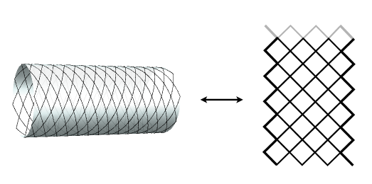
Figure 2.1: The 6-vertex model on a cylinder. In the open channel, there are $2M+1$ sites in the horizontal direction with free boundary conditions, and $2N$ sites in the vertical direction with periodic boundary conditions.

The partition function on the lattice can be computed in two different channels.

Open channel.

In the open channel, we define the diagonal-to-diagonal transfer matrix

$$\mathrm{t}_{D}(u)=\check{R}_{23}(u)\,\check{R}_{45}(u)\cdots\check{R}_{2M,2M+1}(u)\,\check{R}_{12}(u)\,\check{R}_{34}(u)\cdots\check{R}_{2M-1,2M}(u)\,,$$ (2.1)

shown in figure 2.2; by convention the direction of propagation (the “imaginary time” direction) is upwards in our figures.

Figure 2.2: Diagonal-to-diagonal transfer matrix

The subscripts label the spaces being acted upon, and $\check{R}$ is related to the standard $R$-matrix of the isotropic 6-vertex model by

$$\check{R}_{jk}(u)=P_{jk}\,R_{jk}(u)\,,$$ (2.2)

where $P$ is the permutation operator. Written explicitly, the $R$-matrix is given by

$$R(u)=u+iP=\left(\begin{array}[]{cccc}a(u)&0&0&0\\ 0&b(u)&c(u)&0\\ 0&c(u)&b(u)&0\\ 0&0&0&a(u)\\ \end{array}\right)\,,$$ (2.7)

with the Boltzmann weights

$$a(u)=u+i\,,\qquad b(u)=u\,,\qquad c(u)=i\,.$$ (2.8)

The partition function is given by

$$Z(u,M,N)=\mathrm{tr}\,\big{[}\mathrm{t}_{D}(u)^{N}\big{]}\,.$$ (2.9)

For small values of $M$ and $N$, the results can be directly computed by brute force from the definition, for example

$$Z(u,1,1) =2(u+2i)^{2}\,,$$

$$Z(u,1,2) =2\left(u^{4}+8iu^{3}-12u^{2}-8iu+4\right)\,,$$ (2.10)

$$Z(u,2,2) =2\left(u^{8}+16iu^{7}-76u^{6}-184iu^{5}+268u^{4}+256iu^{3}-160u^{2}-64iu+16\right)\,.$$

Closed channel.

In the closed channel, the graph is rotated by $90^{\circ}$ degrees, as shown in figure 2.3.

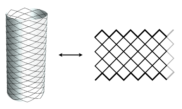
Figure 2.3: In the closed channel, there are $2N$ sites in the horizontal direction with periodic boundary conditions, and $2M+1$ sites in the vertical direction with free boundary conditions.

The rotated $R$-matrix which will be denoted by $R^{\text{c}}$ takes the following form

$$R^{\text{c}}(u)=\left(\begin{array}[]{cccc}b(u)&0&0&0\\ 0&a(u)&c(u)&0\\ 0&c(u)&a(u)&0\\ 0&0&0&b(u)\\ \end{array}\right)\,.$$ (2.15)

Notice that this $R$-matrix does not satisfy the Yang-Baxter equation. In the closed channel, the partition function is no longer given by a trace, since periodic boundary conditions are not imposed in the vertical direction. Instead, the open boundary conditions give rise to non-trivial boundary states in the closed channel. The partition function in the closed channel is given by

$$Z^{\text{c}}(u,M,N)=\langle\Psi_{0}|U^{\dagger}\,\tilde{\mathrm{t}}_{D}(u)^{M}|\Psi_{0}\rangle\,,$$ (2.16)

where $U$ is the one-site shift operator

$$U=P_{12}P_{23}\cdots P_{2N-1,2N}\,,$$ (2.17)

and $\tilde{\mathrm{t}}_{D}(u)$ is defined as

$$\tilde{\mathrm{t}}_{D}(u)=\check{R}^{\text{c}}_{12}(u)\,\check{R}^{\text{c}}_{34}(u)\cdots\check{R}^{\text{c}}_{2N-1,2N}(u)\,\check{R}^{\text{c}}_{23}(u)\,\check{R}^{\text{c}}_{45}(u)\cdots\check{R}^{\text{c}}_{2N-2,2N-1}(u)\,\check{R}^{\text{c}}_{2N,1}(u)\,,$$ (2.18)

where $\check{R}^{\text{c}}_{ij}(u)=P_{ij}R^{\text{c}}_{ij}(u)$. The boundary state $|\Psi_{0}\rangle$ is given by

$$|\Psi_{0}\rangle=|\psi_{0}\rangle^{\otimes N},\qquad|\psi_{0}\rangle=|\uparrow\,\rangle\otimes|\downarrow\,\rangle+|\downarrow\,\rangle\otimes|\uparrow\,\rangle\,,$$ (2.19)

where we have used the notation

$$|\uparrow\,\rangle\equiv{1\choose 0}\,,\qquad|\downarrow\,\rangle\equiv{0\choose 1}\,.$$ (2.20)

The result for the partition function of course does not depend on how we perform the computation, so we have

$$Z(u,M,N)=Z^{\text{c}}(u,M,N)\,.$$ (2.21)

To verify the correctness of our various computations (see below), we have explicitly checked this identity for small value of $M$ and $N$.

Our goal is to compute analytic expressions of $Z(u,M,N)$ explicitly for different intermediate values of $M$ and $N$. When both $M$ and $N$ are large, the system can be well approximated by the computation in the thermodynamic limit. Here we instead focus on the interesting intermediate case where we keep one of $M$, $N$ to be finite (namely, the one that determines the dimension of the transfer matrix) and the other to be large. For finite $M$ ($\leq 10$) and large $N$ (around a few hundred to thousands), we perform the computation in the open channel using (2.9); whereas for finite $N$ and large $M$, we work in the closed channel using (2.16). We discuss the computation of the partition function in both channels from the perspective of Bethe ansatz and algebraic geometry.

3 Partition function in the open channel

In this section, we discuss the computation of the partition function in the open channel using Bethe ansatz and algebraic geometry. Using this method, we are able to compute the partition function for finite $M\leq 10$ and large $N$ (ranging from a few hundred to thousands).

3.1 Reformulation and Bethe ansatz

In order to apply the $R$-matrix machinery, the first step is to re-express the diagonal-to-diagonal transfer matrix $\mathrm{t}_{D}(u)$ (2.1) in terms of an integrable open-chain transfer matrix with $2M+1$ sites and with inhomogeneities $\{\theta_{j}\}$ [11]. Let us define

$$\mathrm{t}(u;\{\theta_{j}\})={\rm tr}_{a}K^{+}(u)\,T_{a}^{(2M+1)}(u;\{\theta_{j}\})\,K^{-}(u)\,\widehat{T}_{a}^{(2M+1)}(u;\{\theta_{j}\})\,,$$ (3.1)

where the monodromy matrices are given by

$$T_{a}^{(l)}(u;\{\theta_{j}\}) =R_{a1}(u-\theta_{1})\ldots R_{a\,l}(u-\theta_{l})\,,$$

$$\widehat{T}_{a}^{(l)}(u;\{\theta_{j}\}) =R_{a\,l}(u+\theta_{l})\ldots R_{a1}(u+\theta_{1})\,.$$ (3.2)

For our isotropic problem, the $K$-matrices are simply $K^{+}(u)=K^{-}(u)=\mathbb{I}$.

The eigenvalues $\Lambda(u;\{\theta_{j}\})$ of the transfer matrix $\mathrm{t}(u;\{\theta_{j}\})$ (3.1), which can be obtained using algebraic Bethe ansatz [11], are given by

$$\Lambda(u;\{\theta_{j}\}) =\frac{2(u+i)}{(2u+i)}\left[\prod_{j=1}^{2M+1}(u-\theta_{j}+i)(u+\theta_{j}+i)\right]\prod_{k=1}^{K}\frac{(u-u_{k}-\frac{i}{2})(u+u_{k}-\frac{i}{2})}{(u-u_{k}+\frac{i}{2})(u+u_{k}+\frac{i}{2})}$$

$$+\frac{2u}{(2u+i)}\left[\prod_{j=1}^{2M+1}(u-\theta_{j})(u+\theta_{j})\right]\prod_{k=1}^{K}\frac{(u-u_{k}+\frac{3i}{2})(u+u_{k}+\frac{3i}{2})}{(u-u_{k}+\frac{i}{2})(u+u_{k}+\frac{i}{2})}\,,$$ (3.3)

where the $\{u_{k}\}$ are solutions of the BAE

$$\prod_{j=1}^{2M+1}\frac{(u_{k}-\theta_{j}+\frac{i}{2})(u_{k}+\theta_{j}+\frac{i}{2})}{(u_{k}-\theta_{j}-\frac{i}{2})(u_{k}+\theta_{j}-\frac{i}{2})}=\prod_{j=1;j\neq k}^{K}\frac{(u_{k}-u_{j}+i)(u_{k}+u_{j}+i)}{(u_{k}-u_{j}-i)(u_{k}+u_{j}-i)}\,.$$ (3.4)

The key point (due to Destri and de Vega [12]) is to choose alternating spectral-parameter-dependent inhomogeneities as follows

$$\theta_{j}=\theta_{j}(u)=(-1)^{j}u\,,\qquad j=1,\ldots,2M+1\,.$$ (3.5)

One can then show [13] that the diagonal-to-diagonal transfer matrix $\mathrm{t}_{D}(u)$ is given by

$$\mathrm{t}_{D}(u)=\frac{1}{i^{2M+1}(u+2i)}\mathrm{t}(\tfrac{u}{2};\{\theta_{j}(\tfrac{u}{2})\})\,,$$ (3.6)

noting that half of the $R$-matrices become proportional to permutation operators, and the spin chain geometry is transformed into the vertex one, see Figure 3.4.

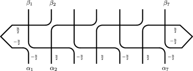
Figure 3.4: The $R$-matrices with zero argument act as permutation operators depicted with avoiding lines. This transforms the double-row transfer matrix of the spin-chain geometry into the diagonal-to-diagonal transfer matrix of the boundary vertex model.

Specifying in (3.3)-(3.4) the inhomogeneities as in (3.5), it follows that the eigenvalues $\Lambda_{D}(u)$ of $\mathrm{t}_{D}(u)$ are given by

$$\Lambda_{D}(u) =\Lambda_{D,K}(u)=\frac{1}{i^{2M+1}(u+2i)}\Lambda(\tfrac{u}{2};\{\theta_{j}(\tfrac{u}{2})\})$$ (3.7)

$$=(u+i)^{2M}\prod_{k=1}^{K}\frac{(\frac{u}{2}-u_{k}-\frac{i}{2})(\frac{u}{2}+u_{k}-\frac{i}{2})}{(\frac{u}{2}-u_{k}+\frac{i}{2})(\frac{u}{2}+u_{k}+\frac{i}{2})}\,,$$ (3.8)

where the $\{u_{k}\}$ are solutions of the Bethe equations

$$\left[\frac{(u_{k}-\frac{u}{2}+\frac{i}{2})(u_{k}+\frac{u}{2}+\frac{i}{2})}{(u_{k}-\frac{u}{2}-\frac{i}{2})(u_{k}+\frac{u}{2}-\frac{i}{2})}\right]^{2M+1} =\prod_{j=1;j\neq k}^{K}\frac{(u_{k}-u_{j}+i)(u_{k}+u_{j}+i)}{(u_{k}-u_{j}-i)(u_{k}+u_{j}-i)}.$$ (3.9)

Here $k=1,\ldots,K$ and $K=0,1,\ldots,M\,$. Note that the BAE (3.9) depend on the spectral parameter $u$, which is an unusual feature.

We observe that $\mathrm{t}_{D}(u)$ has $su(2)$ symmetry

$$\left[\mathrm{t}_{D}(u)\,,\vec{S}\right]=0\,,\qquad\vec{S}=\sum_{j=1}^{2M+1}\tfrac{1}{2}\vec{\sigma}_{j}\,.$$ (3.10)

The Bethe states are $su(2)$ highest-weight states, with spin

$$s=s^{z}=\frac{1}{2}(2M+1)-K\,.$$ (3.11)

For a given value of $K$, the corresponding eigenvalue therefore has degeneracy

$$2s+1=2M+2-2K\,.$$ (3.12)

We conclude that the partition function (2.9) is given by

$$Z(u,M,N)=\sum_{K=0}^{M}\sum_{\text{sol}(M,K)}(2M+2-2K)\,\Lambda_{D,K}(u)^{N}\,,$$ (3.13)

where $\Lambda_{D,K}(u)$ is given by (3.8). Here $\text{sol}(M,K)$ stands for physical solutions $\{u_{1},\ldots,u_{K}\}$ of the BAE (3.9) with $2M+1$ sites and $K$ Bethe roots. The number $\mathcal{N}(M,K)$ of such solutions has been conjectured to be given by [15]

$$\mathcal{N}(M,K)={2M+1\choose K}-{2M+1\choose K-1}\,.$$ (3.14)

In order to find the explicit expressions for the partition function (3.13), we need to find the eigenvalues $\Lambda_{D,K}(u)$. They depend on the values of rapidities which are solutions of the BAE (3.9). We encounter two difficulties. Firstly, the solution set of the BAE (3.9) contains some redundancy, since not all solutions are physical; therefore one needs to impose extra selection rules [15]. Secondly, generally Bethe equations are a complicated system of algebraic equations, which cannot be solved analytically. What is worse, our BAE (3.9) depend on a free parameter $u$, which means that the Bethe roots are functions of $u$, thereby making the BAE even harder than usual to solve.

In order to overcome these two difficulties, we need new tools, namely the rational $Q$-system and computational algebraic geometry. These methods have been applied successfully in computing the torus partition function of the 6-vertex model [7]. The BAE can be reformulated as a set of $QQ$-relations, with appropriate boundary conditions [8]. The benefit of working with the $Q$-system is twofold. Firstly, it is much more efficient to solve the rational $Q$-system than to directly solve the BAE. Secondly, all the solutions of the $Q$-system are physical, so there is no need to impose further selection rules [16, 17]. The rational $Q$-system, which was first developed for isotropic (XXX) spin chains with periodic boundary conditions [8], was recently generalized to anisotropic (XXZ) spin chains and to spin chains with certain open boundary conditions [17, 18]. We briefly review the $Q$-system for open boundary conditions in section 3.2.

Turning to the second difficulty, finding all solutions of the BAE (or of the corresponding $Q$-system) is in general only possible numerically. However, it was realized in [9] that if the goal is to sum over all the solutions of the BAE/$Q$-system for some rational function $f(\{u_{j}\})$ of the Bethe roots, then it can be done without knowing all the solutions explicitly. The idea is based on computational algebraic geometry. The solutions of the BAE/$Q$-system form a finite-dimensional linear space called the quotient ring. The dimension of the quotient ring is the number of physical solutions of the BAE/$Q$-system. A basis of the quotient ring can be constructed by standard methods using a Gröbner basis. Once a basis for the quotient ring is known, one can construct the companion matrix for the function $f(\{u_{j}\})$, which is a finite-dimensional representation of this function in the quotient ring. Taking the trace of the companion matrix gives the sought-after sum. For a more detailed introduction to these notions and explicit examples in the context of toroidal boundary conditions, we refer to the original papers [9, 7] and the textbooks [19, 20].

The same strategy can be applied to the open boundary conditions. The new feature that appears in this case is the dependence on a free parameter $u$. While this creates extra difficulty for numerical computations, it does not cost more effort in the algebro-geometric approach. The reason is that the constructions of the Gröbner basis, the basis for the quotient ring and companion matrices are purely algebraic; and it does not make much qualitative difference whether we have to manipulate numbers or algebraic expressions.

3.2 BAE and $Q$-system

In this section, we review the rational $Q$-system for the $SU(2)$-invariant XXX spin chain with open boundary conditions [18]. Let us first consider the BAE with generic inhomogeneities $\{\theta_{j}\}$ (3.4)

$$\prod_{l=1}^{L}\frac{(u_{j}-\theta_{l}+\tfrac{i}{2})(u_{j}+\theta_{l}+\tfrac{i}{2})}{(u_{j}-\theta_{l}-\tfrac{i}{2})(u_{j}+\theta_{l}-\tfrac{i}{2})}=\prod_{k\neq j}^{K}\frac{(u_{j}-u_{k}+i)(u_{j}+u_{k}+i)}{(u_{j}-u_{k}-i)(u_{j}+u_{k}-i)}\,,$$ (3.15)

where $L=2M+1$. For given value of $L$ and $K$, we consider a two-row Young tableau with number of boxes $(L-K,K)$. At each vertex of the Young tableau, we associate a $Q$-function denoted by $Q_{a,s}$. The BAE (3.15) can be obtained from the following $QQ$-relations

$$v\,Q_{a+1,s}(v)\,Q_{a,s+1}(v)\propto Q^{+}_{a+1,s+1}(v)\,Q^{-}_{a,s}(v)-Q^{-}_{a+1,s+1}(v)\,Q^{+}_{a,s}(v)\,,$$ (3.16)

where $f^{\pm}(v):=f(v\pm\frac{i}{2})$, and the $Q$-functions $Q_{a,s}(v)$ are even polynomials of $v$

$$Q_{a,s}(v)=v^{2M_{a,s}}+\sum_{k=0}^{M_{a,s}-1}c_{a,s}^{(k)}\,v^{2k}\,,$$ (3.17)

where $M_{a,s}$ is the number of boxes in the Young tableau to the right and top of the vertex $(a,s)$. The boundary conditions are chosen such that $Q_{2,s}=1$, $Q_{1,s>K}=1$ and

$$Q_{0,0}(v)= \,\prod_{j=1}^{L}(v-\theta_{j})(v+\theta_{j})\,,$$

$$Q_{1,0}(v)= \,Q(v)=\prod_{k=1}^{K}(v-u_{k})(v+u_{k})\,.$$ (3.18)

Here $Q_{1,0}(v)$ is the usual Baxter $Q$-function, whose zeros are the Bethe roots. Comparing to the periodic $QQ$-relations [8], the main differences are an extra factor $v$ that appears on the left-hand side of (3.16), and the degree of the polynomial of $Q_{a,s}$ which is twice the one for the periodic case. More details can be found in section 4.2 of [18].

For the Bethe equations (3.9), corresponding to the alternating inhomogeneities (3.5), we simply have

$$Q_{0,0}(v)=\left[(v-\tfrac{u}{2})(v+\tfrac{u}{2})\right]^{2M+1}\,.$$ (3.19)

To solve the $Q$-system, we impose the condition that all the $Q_{a,s}$ functions are polynomials. This requirement generates a set of algebraic equations called zero remainder conditions (ZRC) for the coefficients $c_{a,s}^{(k)}$. In principle, one can then solve the ZRC’s and find $Q_{a,s}$, in particular the main $Q$-function $Q_{1,0}$. The zeros of $Q_{1,0}$ are the Bethe roots $\{u_{k}\}$, which are functions of the parameter $u$.

After finding the $Q$-functions, the next step is to find the eigenvalues $\Lambda_{D}$ (3.8), which in terms of $Q$-functions are given simply by

$$\Lambda_{D}(u)=(u+i)^{2M}\frac{Q(\frac{u}{2}-\frac{i}{2})}{Q(\frac{u}{2}+\frac{i}{2})}\,.$$ (3.20)

Plugging these into (3.13), we finally obtain the partition function.

3.3 Algebraic geometry

In this subsection, we give the main steps for the algebro-geometric computation of the partition function:

1. Generate the set of zero remainder conditions (ZRC) from the rational $Q$-system;

2. Compute the Gröbner basis of the ZRC;

3. Construct the quotient ring of the ZRC;

4. Compute the companion matrix for the eigenvalues $\Lambda_{D,K}(u)$ (3.8) which will be denoted by $\mathbb{T}_{M,K}(u)$;

5. Compute the matrix power of $\mathbb{T}_{M,K}(u)$ and take the trace

   $$Z(u,M,N)=\sum_{K=0}^{M}(2M+2-2K)\,{\rm tr}\left[\mathbb{T}_{M,K}(u)\right]^{N}\,.$$ (3.21)

Most steps listed above can be done straightforwardly, adapting the corresponding working of [7]. The only step that requires some additional work is step 4. The variables of ZRC are $c_{a,s}^{(k)}$ which are coefficients of the $Q$-functions. From these variables, it is easy to construct the companion matrix of the $Q$-function. For fixed $M$ and $K$, we denote the companion matrix by $\mathbb{Q}_{M,K}$. To find the companion matrix of $\Lambda_{D}$, which is essentially the companion matrix of $\Lambda$ (3.20) up to some multiplicative factors, the most direct way is to use homomorphism property of the companion matrix and write

$$\mathbb{T}_{M,K}(u)= \,(u+i)^{2M}\frac{\mathbb{Q}_{M,K}(\tfrac{u}{2}-\tfrac{i}{2})}{\mathbb{Q}_{M,K}(\tfrac{u}{2}+\tfrac{i}{2})}\,,$$ (3.22)

where $\mathbb{T}_{M,K}(u)$ is the companion matrix for $\Lambda_{D}(u)$ with fixed $M$ and $K$. Unfortunately, this method involves taking the inverse of the matrix $\mathbb{Q}_{M,K}(u+\tfrac{i}{2})$ analytically, which can be slow when the dimension of the matrix is large.

We find that a much more efficient way is to use the following $TQ$-relation

$$u\,T(u-\tfrac{i}{2})Q(u)= \,(u+\tfrac{i}{2})\left[(u+\tfrac{i}{2})^{2}-(\tfrac{z}{2})^{2}\right]^{L}Q(u-i)$$ (3.23)

$$+(u-\tfrac{i}{2})\left[(u-\tfrac{i}{2})^{2}-(\tfrac{z}{2})^{2}\right]^{L}Q(u+i).$$

In our case, we need to take $L=2M+1$ and $z=u$. To solve the $TQ$ relation (3.23), we make the following ansatz for the two polynomials

$$T(u)= \,t_{2L}u^{2L}+t_{2L-1}u^{2L-1}+\cdots+t_{0},$$ (3.24)

$$Q(u)= \,u^{2K}+s_{K-1}u^{2(K-1)}+\cdots+s_{0}.$$

Notice that $Q(u)$ is an even polynomial and only even powers of $u$ appear, which is not the case for $T(u)$. Plugging the ansatz (3.24) into (3.23), we obtain a system of algebraic equations for the coefficients $\{t_{0},t_{1},\cdots,t_{2L},s_{0},\cdots,s_{K-1}\}$. In fact, solving these set of algebraic equations is yet another way to find the Bethe roots. For our purpose, we only solve the equation partially, namely we view $\{s_{0},\cdots,s_{K-1}\}$ as parameters and solve $\{t_{k}\}$ in terms of $\{s_{j}\}$. This turns out to be much simpler since the equations are linear. We find that $t_{k}(\{s_{j}\})$ are polynomials in the variables $\{s_{j}\}$. From ZRC and algebro-geometric computations, we can find the companion matrix of $s_{j}$ which we denote by $\mathbf{s}_{j}$. Replacing $s_{j}$ by $\mathbf{s}_{j}$ and the products by matrix multiplication in $t_{k}(\{s_{j}\})$, we find the companion matrix $\mathbf{t}_{k}=t_{k}(\{\mathbf{s}_{j}\})$. Then the companion matrix of the eigenvalues of the transfer matrix is given by

$$\mathbb{T}_{M,K}(u)=\mathbf{t}_{2L}\,u^{2L}+\mathbf{t}_{2L-1}\,u^{2L-1}+\cdots+\mathbf{t}_{0}.$$ (3.25)

More details on the implementation of the algebro-geometric computations are given in appendix B.

Using the AG approach, we have computed the partition functions for $M$ up to $6$, with $N$ up to $2048$. We also calculated some partition functions with higher $M$ and lower $N$. The results for $2\leq M,N\leq 6$ are given in Appendix F.

4 Partition function in the closed channel

In this section, we compute the partition function in the closed channel. There are both simplifications and complications due to the presence of non-trivial boundary states. Indeed, the presence of boundary states imposes selection rules for the allowed solutions of the BAE. Firstly, it restricts to the states with zero total spin. This implies that the length of the spin chain must be even, which we denote by $2N$; and the only allowed number of Bethe roots is $K=N$. In contrast, for the periodic (torus) case [7], one must consider all the sectors $K=0,1,\ldots,N$. Moreover, the Bethe roots must form Cooper-type pairs (4.35), which leads to significant simplification in the computation of the Gröbner basis and quotient ring.

This simplification comes with a price. Recall that the partition function in the closed channel takes the form of a matrix element given by (2.16). To evaluate this matrix element, we need the overlaps between the boundary states and the Bethe states. These overlaps are a new feature, which is not present in the open channel. They are complicated functions of the rapidities, which makes the computation of the companion matrix more difficult.

4.1 Reformulation and Bethe ansatz

To compute the expression (2.16) for the partition function in the closed channel, the first step is to rewrite $\tilde{\mathrm{t}}_{D}$ (2.18) in terms of integrable closed-chain transfer matrices. To this end, we observe that ${R}^{\text{c}}(u)$ (2.15) is related to $R(u)$ by

$${R}^{\text{c}}_{12}(u)=-\sigma_{1}^{z}\,R_{12}(\tilde{u})\,\sigma_{1}^{z}=-\sigma_{2}^{z}\,R_{12}(\tilde{u})\,\sigma_{2}^{z}\,,$$ (4.1)

where $\tilde{u}$ is the ‘crossing transformed’ spectral parameter defined by

$$\tilde{u}=-u-i\,.$$ (4.2)

The corresponding “checked” $R$-matrices are therefore related by

$$\check{{R}}^{\text{c}}_{12}(u)=-\sigma_{2}^{z}\,\check{R}_{12}(\tilde{u})\,\sigma_{2}^{z}\,.$$ (4.3)

For later convenience, we define

$$\tilde{V}^{(1)}= \,\check{R}^{\text{c}}_{23}(u)\,\check{R}^{\text{c}}_{45}(u)\cdots\check{R}^{\text{c}}_{2N-2,2N-1}(u)\,\check{R}^{\text{c}}_{2N,1}(u)\,,$$

$$\tilde{V}^{(2)}= \,\check{R}^{\text{c}}_{12}(u)\,\check{R}^{\text{c}}_{34}(u)\cdots\check{R}^{\text{c}}_{2N-1,2N}(u)\,,$$ (4.4)

in terms of which $\tilde{\mathrm{t}}_{D}$ (2.18) is given by

$$\tilde{\mathrm{t}}_{D}(u)=\tilde{V}^{(2)}(u)\,\tilde{V}^{(1)}(u)\,.$$ (4.5)

It follows from (4.3) that

$$\tilde{V}^{(1)}(u) =(-1)^{N}\,\Omega^{(2)}\,V^{(1)}(\tilde{u})\,\Omega^{(1)}\,,$$

$$\tilde{V}^{(2)}(u) =(-1)^{N}\,\Omega^{(1)}\,V^{(2)}(\tilde{u})\,\Omega^{(2)}\,,$$ (4.6)

where

$$\Omega^{(1)}=\sigma^{z}_{1}\sigma^{z}_{3}\cdots\sigma^{z}_{2N-1}\,,\qquad\Omega^{(2)}=\sigma^{z}_{2}\sigma^{z}_{4}\cdots\sigma^{z}_{2N}\,,$$ (4.7)

and the $V^{(i)}$ are the same as the corresponding $\tilde{V}^{(i)}$, but with $R$’s instead of ${R}^{\text{c}}$’s:

$$V^{(1)}(u) =\check{R}_{23}(u)\,\check{R}_{45}(u)\,\ldots\check{R}_{2N-2,2N-1}(u)\,\check{R}_{2N,1}(u)\,,$$

$$V^{(2)}(u) =\check{R}_{12}(u)\,\check{R}_{34}(u)\,\ldots\check{R}_{2N-1,2N}(u)\,.$$ (4.8)

Let us now introduce integrable inhomogeneous closed-chain transfer matrices of length $2N$

$$\tau(u;\{\theta_{j}\}) ={\rm tr}_{a}T_{a}^{(2N)}(u;\{\theta_{j}\})\,,$$

$$\widehat{\tau}(u;\{\theta_{j}\}) ={\rm tr}_{a}\widehat{T}_{a}^{(2N)}(u;\{\theta_{j}\})\,,$$ (4.9)

where the monodromy matrices are defined in (3.2). Using crossing symmetry

$$R_{12}(\tilde{u})=-\sigma_{1}^{y}\,R_{12}^{t_{1}}(u)\,\sigma_{1}^{y}\,,$$ (4.10)

where ‘$t_{1}$’ stands for transposition in the first quantum space, one can show that

$$\tau(\tilde{u};\{\theta_{j}\})=\widehat{\tau}(u;\{\theta_{j}\})\,.$$ (4.11)

The transfer matrices (4.9) can be diagonalized by algebraic Bethe ansatz. We define the operators $A$, $B$, $C$, $D$ as matrix elements of the monodromy matrix (3.2) as usual

$$T_{a}^{(2N)}(u-\tfrac{i}{2};\{\theta_{j}\})=\left(\begin{array}[]{cc}A(u)&B(u)\\ C(u)&D(u)\\ \end{array}\right)\,,$$ (4.14)

but note the shift in the spectral parameter. We consider the reference state or pseudovacuum

$$|0\rangle=|\uparrow\rangle^{\otimes 2N}\,.$$ (4.15)

The Bethe states and their duals are constructed by acting with $B$- and $C$-operators on the reference state

$$|\mathbf{u}\rangle=B(u_{1})\cdots B(u_{K})|0\rangle\,,\qquad\langle\mathbf{u}|=\langle 0|C(u_{1})\cdots C(u_{K})\,.$$ (4.16)

These states are eigenstates of the transfer matrix $\tau(u;\{\theta_{j}\})$ (4.9)

$$\tau(u;\{\theta_{j}\})|\mathbf{u}\rangle=\Lambda_{c}(u;\{\theta_{j}\})|\mathbf{u}\rangle\,,$$ (4.17)

with eigenvalues $\Lambda_{c}(u;\{\theta_{j}\})$ given by

$$\Lambda_{c}(u;\{\theta_{j}\})=\prod_{j=1}^{2N}(u-\theta_{j}+i)\prod_{k=1}^{K}\frac{u-u_{k}-\tfrac{i}{2}}{u-u_{k}+\tfrac{i}{2}}+\prod_{j=1}^{2N}(u-\theta_{j})\prod_{k=1}^{K}\frac{u-u_{k}+\tfrac{3i}{2}}{u-u_{k}+\tfrac{i}{2}}\,,$$ (4.18)

provided that the rapidities $\mathbf{u}=\{u_{1},\cdots,u_{K}\}$ satisfy the BAE

$$\prod_{j=1}^{2N}\frac{u_{k}-\theta_{j}+\tfrac{i}{2}}{u_{k}-\theta_{j}-\tfrac{i}{2}}=\prod_{j=1;j\neq k}^{K}\frac{u_{k}-u_{j}+i}{u_{k}-u_{j}-i}\,.$$ (4.19)

In contradistinction with (3.9) these BAE do not depend on the spectral parameter $u$, as is usually the case. The eigenvalues $\widehat{\Lambda}_{c}(u;\{\theta_{j}\})$ of $\widehat{\tau}(u;\{\theta_{j}\})$ are given by

$$\widehat{\Lambda}_{c}(u;\{\theta_{j}\})=\Lambda_{c}(\tilde{u};\{\theta_{j}\})\,,$$ (4.20)

as follows from (4.11).

To make contact with $\tilde{\mathrm{t}}_{D}$, we again choose alternating spectral-parameter-dependent inhomogeneities

$$\theta_{j}=\theta_{j}(u)=(-1)^{j+1}u,\qquad j=1,\ldots,2N\,.$$ (4.21)

The $V$’s (4.8) can then be related to the closed-chain transfer matrices (4.9) by

$$V^{(2)}(u)\,V^{(1)}(u)=(-1)^{N}\,\tau(\tfrac{u}{2};\{\theta_{j}(\tfrac{u}{2})\})\,\widehat{\tau}(\tfrac{u}{2};\{\theta_{j}(\tfrac{u}{2})\})\,,$$ (4.22)

which is similar to (3.6), see Figure 4.5.

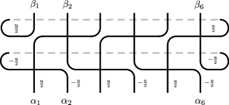
Figure 4.5: The $R$-matrices with zero argument act as permutation operators depicted with avoiding lines. This transforms the product of periodic transfer matrices of the spin-chain geometry into the periodic diagonal-to-diagonal transfer matrix of the vertex model.

In view of the relations (4.6) between $\tilde{V}$’s and $V$’s, we conclude that $\tilde{\mathrm{t}}_{D}$ (4.5) is given by

$$\tilde{\mathrm{t}}_{D}(u) =\tilde{V}^{(2)}(u)\,\tilde{V}^{(1)}(u)$$

$$=\Omega^{(1)}\,V^{(2)}(\tilde{u})\,V^{(1)}(\tilde{u})\,\Omega^{(1)}$$

$$=(-1)^{N}\Omega^{(1)}\,\tau(\tfrac{\tilde{u}}{2};\{\theta_{j}(\tfrac{\tilde{u}}{2})\})\,\widehat{\tau}(\tfrac{\tilde{u}}{2};\{\theta_{j}(\tfrac{\tilde{u}}{2})\})\,\Omega^{(1)}\,.$$ (4.23)

The expression (2.16) for the partition function in the closed channel can therefore be recast as

$$Z^{\text{c}}(u,M,N) =(-1)^{MN}\langle\Psi_{0}|U^{\dagger}\Omega^{(1)}\left[\tau(\tfrac{\tilde{u}}{2};\{\theta_{j}(\tfrac{\tilde{u}}{2})\})\,\widehat{\tau}(\tfrac{\tilde{u}}{2};\{\theta_{j}(\tfrac{\tilde{u}}{2})\})\right]^{M}\Omega^{(1)}|\Psi_{0}\rangle$$

$$=(-1)^{(M+1)N}\langle\Phi_{0}|U^{\dagger}\left[\tau(\tfrac{\tilde{u}}{2};\{\theta_{j}(\tfrac{\tilde{u}}{2})\})\,\widehat{\tau}(\tfrac{\tilde{u}}{2};\{\theta_{j}(\tfrac{\tilde{u}}{2})\})\right]^{M}|\Phi_{0}\rangle\,,$$ (4.24)

where $|\Phi_{0}\rangle$ is the so-called dimer state

$$|\Phi_{0}\rangle=\Omega^{(1)}|\Psi_{0}\rangle=(-1)^{N}\,\Omega^{(2)}|\Psi_{0}\rangle=|\phi_{0}\rangle^{\otimes N},\qquad|\phi_{0}\rangle=|\uparrow\,\rangle\otimes|\downarrow\,\rangle-|\downarrow\,\rangle\otimes|\uparrow\,\rangle,$$ (4.25)

and we have also used the fact that $U^{\dagger}\Omega^{(1)}U=\Omega^{(2)}$. We now insert in (4.24) the completeness relation in terms of Bethe states (which are $SU(2)$ highest-weight states) and their lower-weight descendants

$$\sum_{K}\sum_{\text{sol}_{\rm c}(N,K)}\frac{1}{{\cal N}(\mathbf{u})}|\mathbf{u}\rangle\langle\mathbf{u}|+\ldots={\bf 1}\,,$$ (4.26)

where $\text{sol}_{\rm c}(N,K)$ stands for physical solutions $\mathbf{u}$ of the closed-chain BAE (4.19) with $2N$ sites and $K$ Bethe roots. Moreover, the normalization factor is given by

$${\cal N}(\mathbf{u})=\langle\mathbf{u}|\mathbf{u}\rangle\,,$$ (4.27)

and the ellipsis denotes the descendant terms. However, these descendant terms do not contribute to the matrix element (4.24), since the dimer state is annihilated by the spin raising and lowering operators

$$S^{\pm}\,|\Phi_{0}\rangle=0\,,\qquad\text{where}\qquad S^{\pm}=S^{x}\pm iS^{y}\,,\qquad\vec{S}=\sum_{j=1}^{2N}\tfrac{1}{2}\vec{\sigma}_{j}\,.$$ (4.28)

Moreover, in view of the fact

$$0=\langle\mathbf{u}|S^{z}|\Phi_{0}\rangle=(N-K)\langle\mathbf{u}|\Phi_{0}\rangle\,,$$ (4.29)

the overlap $\langle\mathbf{u}|\Phi_{0}\rangle$ vanishes unless $K=N$. The matrix element (4.24) therefore reduces to

$$Z^{\text{c}}(u,M,N) =(-1)^{(M+1)N}\sum_{\text{sol}_{c}(N,N)}\frac{\langle\Phi_{0}|U^{\dagger}|\mathbf{u}\rangle\langle\mathbf{u}|\Phi_{0}\rangle}{{\cal N}(\mathbf{u})}\left[\Lambda_{\rm c}(\tfrac{\tilde{u}}{2};\{\theta_{j}(\tfrac{\tilde{u}}{2})\})\,\widehat{\Lambda}_{c}(\tfrac{\tilde{u}}{2};\{\theta_{j}(\tfrac{\tilde{u}}{2})\})\right]^{M}\,,$$ (4.30)

where the sum runs over all physical solutions of the closed-chain BAE (4.19) in the $K=N$ sector. We note that the expressions involving the eigenvalues are given by

$$\Lambda_{\rm c}(\tfrac{\tilde{u}}{2};\{\theta_{j}(\tfrac{\tilde{u}}{2})\}) =(-iu)^{N}\prod_{k=1}^{N}\frac{-\frac{u}{2}-u_{k}-i}{-\frac{u}{2}-u_{k}}\,,$$

$$\widehat{\Lambda}_{c}(\tfrac{\tilde{u}}{2};\{\theta_{j}(\tfrac{\tilde{u}}{2})\}) =(-iu)^{N}\prod_{k=1}^{N}\frac{\frac{u}{2}-u_{k}+i}{\frac{u}{2}-u_{k}}\,,$$ (4.31)

as follows from (4.18) and (4.20). The normalization factor (4.27) is given by the Gaudin formula [21, 22]

$${\cal N}(\mathbf{u}) =(-1)^{N}\prod_{j=1}^{N}\left[\left(u_{j}+\tfrac{\tilde{u}}{2}\right)^{2}+\tfrac{1}{4}\right]^{N}\left[\left(u_{j}-\tfrac{\tilde{u}}{2}\right)^{2}+\tfrac{1}{4}\right]^{N}\left[\prod_{j,k=1\,;j\neq k}^{N}\frac{u_{j}-u_{k}-i}{u_{j}-u_{k}}\right]\,{\rm det}{}_{N}\left(G_{jk}\right)\,,$$ (4.32)

where

$$G_{jk}=\delta_{jk}\left\{N\left[K_{\frac{1}{2}}(u_{j}-\tfrac{\tilde{u}}{2})+K_{\frac{1}{2}}(u_{j}+\tfrac{\tilde{u}}{2})\right]-\sum_{l=1}^{N}K_{1}(u_{j}-u_{l})\right\}+K_{1}(u_{j}-u_{k})\,,$$ (4.33)

and

$$K_{a}(u)=\frac{2a}{u^{2}+a^{2}}\,.$$ (4.34)

Overlaps similar to $\langle\mathbf{u}|\Phi_{0}\rangle$ have been studied extensively, see e.g. [23, 24, 25, 26, 27, 28, 29, 30], see also [31, 32]. The cases of even and odd $N$ must be analyzed separately.

4.2 Even $N$

Let us first consider even values of $N$. Interestingly, only Bethe states with “paired” Bethe roots of the form

$$\{u_{1}\,,-u_{1}\,,\ldots\,,u_{\frac{N}{2}}\,,-u_{\frac{N}{2}}\}$$ (4.35)

have non-zero overlaps [25, 26]. Such Bethe states have even parity, see (E.5) below. For such Bethe states, the overlaps are given by (see Appendix C)

$$\langle\mathbf{u}|\Phi_{0}\rangle=\left(\tfrac{\tilde{u}}{2}+\tfrac{i}{2}\right)^{N}\,\left[\prod_{j=1}^{\frac{N}{2}}\frac{1}{u_{j}\sqrt{u_{j}^{2}+\frac{1}{4}}}\right]\sqrt{\frac{{\rm det}{}_{\frac{N}{2}}\left(G^{+}_{jk}\right)}{{\rm det}{}_{\frac{N}{2}}\left(G^{-}_{jk}\right)}}\sqrt{{\cal N}(\mathbf{u})}\,,$$ (4.36)

where

$$G^{\pm}_{jk}=\delta_{jk}\left\{N\left[K_{\frac{1}{2}}(u_{j}-\tfrac{\tilde{u}}{2})+K_{\frac{1}{2}}(u_{j}+\tfrac{\tilde{u}}{2})\right]-\sum_{l=1}^{\frac{N}{2}}K^{(+)}_{1}(u_{j}\,,u_{l})\right\}+K^{(\pm)}_{1}(u_{j}\,,u_{k})\,,$$ (4.37)

with

$$K^{(\pm)}_{a}(u,v)=K_{a}(u-v)\pm K_{a}(u+v)\,,$$ (4.38)

and $K_{a}(u)$ is defined in (4.34). We remark that, for these states,

$${\rm det}{}_{N}\left(G_{jk}\right)={\rm det}{}_{\frac{N}{2}}\left(G^{+}_{jk}\right)\,{\rm det}{}_{\frac{N}{2}}\left(G^{-}_{jk}\right)\,.$$ (4.39)

Moreover, we show in Appendix D the relation

$$\langle\Phi_{0}|U^{\dagger}|\mathbf{u}\rangle=i^{N}(\tilde{u}+i)^{-N}\Lambda_{\rm c}(\tfrac{\tilde{u}}{2};\{\theta_{j}(\tfrac{\tilde{u}}{2})\})\langle\mathbf{u}|\Phi_{0}\rangle\,.$$ (4.40)

The matrix element (4.30) therefore reduces to

$$Z^{\text{c}}(u,M,N) =\frac{i^{N}(-1)^{(M+1)N}}{2^{2N}}(\tilde{u}+i)^{N}\sum_{\text{sol}(u_{1},\ldots,u_{\frac{N}{2}})}\left[\prod_{j=1}^{\frac{N}{2}}\frac{1}{u_{j}^{2}\left(u_{j}^{2}+\frac{1}{4}\right)}\right]\frac{{\rm det}{}_{\frac{N}{2}}\left(G^{+}_{jk}\right)}{{\rm det}{}_{\frac{N}{2}}\left(G^{-}_{jk}\right)}$$

$$\qquad\qquad\times\Lambda_{\rm c}(\tfrac{\tilde{u}}{2};\{\theta_{j}(\tfrac{\tilde{u}}{2})\})\left[\Lambda_{\rm c}(\tfrac{\tilde{u}}{2};\{\theta_{j}(\tfrac{\tilde{u}}{2})\})\,\widehat{\Lambda}_{c}(\tfrac{\tilde{u}}{2};\{\theta_{j}(\tfrac{\tilde{u}}{2})\})\right]^{M}\,,$$

$$=2^{-2N}u^{2N(M+1)}\sum_{\text{sol}(u_{1},\ldots,u_{\frac{N}{2}})}\left[\prod_{j=1}^{\frac{N}{2}}\frac{1}{u_{j}^{2}\left(u_{j}^{2}+\frac{1}{4}\right)}\right]\frac{{\rm det}{}_{\frac{N}{2}}\left(G^{+}_{jk}\right)}{{\rm det}{}_{\frac{N}{2}}\left(G^{-}_{jk}\right)}$$

$$\qquad\qquad\times\left[\prod_{k=1}^{\frac{N}{2}}\left(\frac{\frac{u}{2}-u_{k}+i}{\frac{u}{2}-u_{k}}\right)\left(\frac{\frac{u}{2}+u_{k}+i}{\frac{u}{2}+u_{k}}\right)\right]^{2M+1}\,,$$ (4.41)

where we have used (4.31) to pass to the second equality, and the sum is over all physical solutions of the BAE (4.19) with paired Bethe roots (4.35), see (4.52) below.

4.3 Odd $N$

For odd values of $N$, the only Bethe states with non-zero overlaps have one 0 Bethe root, and all the other Bethe roots form pairs; i.e., the Bethe roots are of the form

$$\{u_{1}\,,-u_{1}\,,\ldots\,,u_{\frac{N-1}{2}}\,,-u_{\frac{N-1}{2}}\,,0\}\,.$$ (4.42)

Such Bethe states have odd parity, see (E.6) below. The overlaps are now given by

$$\langle\mathbf{u}|\Phi_{0}\rangle=-\left(\tfrac{\tilde{u}}{2}+\tfrac{i}{2}\right)^{N}\,\left[\prod_{j=1}^{\frac{N-1}{2}}\frac{1}{u_{j}\sqrt{u_{j}^{2}+\frac{1}{4}}}\right]\sqrt{\frac{{\rm det}{}_{\frac{N+1}{2}}\left(H_{jk}\right)}{{\rm det}{}_{\frac{N-1}{2}}\left(G^{-}_{jk}\right)}}\sqrt{{\cal N}(\mathbf{u})}\,,$$ (4.43)

where $H$ is the block matrix

$$H=\left(\begin{array}[]{cc}G^{+}&2C\\ C^{t}&D\end{array}\right)_{\frac{N+1}{2}\times\frac{N+1}{2}}\,,$$ (4.46)

and $G^{\pm}$ are now the $\frac{N-1}{2}\times\frac{N-1}{2}$ matrices given by

$$G^{\pm}_{jk} =\delta_{jk}\left\{N\left[K_{\frac{1}{2}}(u_{j}-\tfrac{\tilde{u}}{2})+K_{\frac{1}{2}}(u_{j}+\tfrac{\tilde{u}}{2})\right]-K_{1}(u_{j})-\sum_{l=1}^{\frac{N-1}{2}}K^{(+)}_{1}(u_{j}\,,u_{l})\right\}$$

$$\qquad\qquad\qquad\qquad+K^{(\pm)}_{1}(u_{j}\,,u_{k})\,,\qquad\qquad j\,,k=1,\ldots\,,\frac{N-1}{2}\,,$$ (4.47)

with $K^{(\pm)}_{a}(u,v)$ and $K_{a}(u)$ defined as before, see (4.38), (4.34). Moreover, in (4.46), $C$ is an $\frac{N-1}{2}$-component column vector, $C^{t}$ is the corresponding row vector, and $D$ is a scalar, which are given by

$$C_{j} =K_{1}(u_{j})\,,\qquad j=1,\ldots\,,\frac{N-1}{2}\,,$$

$$D =2NK_{\frac{1}{2}}(\tfrac{\tilde{u}}{2})-2\sum_{l=1}^{\frac{N-1}{2}}K_{1}(u_{l})\,.$$ (4.48)

We remark that, for these states,

$${\rm det}{}_{N}\left(G_{jk}\right)={\rm det}{}_{\frac{N+1}{2}}\left(H_{jk}\right)\,{\rm det}{}_{\frac{N-1}{2}}\left(G^{-}_{jk}\right)\,.$$ (4.49)

Moreover,

$$\langle\Phi_{0}|U^{\dagger}|\mathbf{u}\rangle=i^{N}(\tilde{u}+i)^{-N}\Lambda_{\rm c}(\tfrac{\tilde{u}}{2};\{\theta_{j}(\tfrac{\tilde{u}}{2})\})\langle\mathbf{u}|\Phi_{0}\rangle\,.$$ (4.50)

The matrix element (4.30) now reduces to

$$Z^{\text{c}}(u,M,N) =\frac{i^{N}(-1)^{(M+1)N}}{2^{2N}}(\tilde{u}+i)^{N}\sum_{\text{sol}(u_{1},\ldots,u_{\frac{N-1}{2}})}\left[\prod_{j=1}^{\frac{N-1}{2}}\frac{1}{u_{j}^{2}\left(u_{j}^{2}+\frac{1}{4}\right)}\right]\frac{{\rm det}{}_{\frac{N+1}{2}}\left(H_{jk}\right)}{{\rm det}{}_{\frac{N-1}{2}}\left(G^{-}_{jk}\right)}$$

$$\qquad\qquad\times\Lambda_{\rm c}(\tfrac{\tilde{u}}{2};\{\theta_{j}(\tfrac{\tilde{u}}{2})\})\left[\Lambda_{\rm c}(\tfrac{\tilde{u}}{2};\{\theta_{j}(\tfrac{\tilde{u}}{2})\})\,\widehat{\Lambda}_{c}(\tfrac{\tilde{u}}{2};\{\theta_{j}(\tfrac{\tilde{u}}{2})\})\right]^{M}\,,$$

$$=2^{-2N}u^{2N(M+1)}\sum_{\text{sol}(u_{1},\ldots,u_{\frac{N-1}{2}})}\left[\prod_{j=1}^{\frac{N-1}{2}}\frac{1}{u_{j}^{2}\left(u_{j}^{2}+\frac{1}{4}\right)}\right]\frac{{\rm det}{}_{\frac{N+1}{2}}\left(H_{jk}\right)}{{\rm det}{}_{\frac{N-1}{2}}\left(G^{-}_{jk}\right)}$$

$$\qquad\qquad\times\left[\left(\frac{u+2i}{u}\right)\prod_{k=1}^{\frac{N-1}{2}}\left(\frac{\frac{u}{2}-u_{k}+i}{\frac{u}{2}-u_{k}}\right)\left(\frac{\frac{u}{2}+u_{k}+i}{\frac{u}{2}+u_{k}}\right)\right]^{2M+1}\,,$$ (4.51)

where we have used (4.31) to pass to the second equality, and the sum is over all physical solutions of the BAE (4.19) with paired Bethe roots (4.42), see (4.57) below.

4.4 BAE and $Q$-system

We now summarize the BAE and $Q$-systems in the closed channel. They are special cases of those for the spin chain with periodic boundary condition with length $2N$ and magnon number $N$.

Even $N$.

For the paired Bethe roots (4.35), the closed-chain Bethe equations (4.19) reduce to open-chain-like Bethe equations

$$\left(\frac{u_{k}-\tfrac{\tilde{u}}{2}+\frac{i}{2}}{u_{k}-\tfrac{\tilde{u}}{2}-\frac{i}{2}}\right)^{N}\left(\frac{u_{k}+\tfrac{\tilde{u}}{2}+\frac{i}{2}}{u_{k}+\tfrac{\tilde{u}}{2}-\frac{i}{2}}\right)^{N} =\left(\frac{u_{k}+\frac{i}{2}}{u_{k}-\frac{i}{2}}\right)\prod_{j=1;j\neq k}^{\frac{N}{2}}\left(\frac{u_{k}-u_{j}+i}{u_{k}-u_{j}-i}\right)\left(\frac{u_{k}+u_{j}+i}{u_{k}+u_{j}-i}\right)\,,$$ (4.52)

where $k=1,\ldots,\frac{N}{2}$. The corresponding $QQ$-relations are

$$Q_{a+1,s}(v)\,Q_{a,s+1}(v)\propto Q^{+}_{a+1,s+1}(v)\,Q^{-}_{a,s}(v)-Q^{-}_{a+1,s+1}(v)\,Q^{+}_{a,s}(v)\,,$$ (4.53)

where $Q_{a,s}(v)$ are even polynomial functions of $v$. In particular, the main $Q$-function is given by

$$Q_{1,0}(v)=\prod_{j=1}^{\frac{N}{2}}(v-u_{j})(v+u_{j})=\sum_{k=0}^{\frac{N}{2}}c_{1,0}^{(2k)}v^{2k}=v^{N}+c_{1,0}^{(N-2)}v^{N-2}+\cdots+c_{1,0}^{(0)}\,.$$ (4.54)

Moreover,

$$Q_{0,0}(v)=\left[(v-\tfrac{\tilde{u}}{2})(v+\tfrac{\tilde{u}}{2})\right]^{N}\,.$$ (4.55)

Therefore, to obtain the ZRC for this case, we can simply take the ZRC for the generic periodic case and add the following constraints

$$c_{1,0}^{(2k+1)}=0,\qquad k=0,1,\ldots,\tfrac{N}{2}-1.$$ (4.56)

Odd $N$.

For odd $N$, the nonzero paired Bethe roots (4.42) satisfy the open-chain-like Bethe equations

$$\left(\frac{u_{k}-\tfrac{\tilde{u}}{2}+\frac{i}{2}}{u_{k}-\tfrac{\tilde{u}}{2}-\frac{i}{2}}\right)^{N}\left(\frac{u_{k}+\tfrac{\tilde{u}}{2}+\frac{i}{2}}{u_{k}+\tfrac{\tilde{u}}{2}-\frac{i}{2}}\right)^{N} =\left(\frac{u_{k}+\frac{i}{2}}{u_{k}-\frac{i}{2}}\right)\left(\frac{u_{k}+i}{u_{k}-i}\right)\prod_{j=1;j\neq k}^{\frac{N-1}{2}}\left(\frac{u_{k}-u_{j}+i}{u_{k}-u_{j}-i}\right)\left(\frac{u_{k}+u_{j}+i}{u_{k}+u_{j}-i}\right)\,,$$ (4.57)

where $k=1,\ldots,(N-1)/2$. The corresponding $QQ$-relations are again given by (4.53), with $Q_{0,0}(v)$ given by (4.55). The $Q$-functions are odd polynomials in this case. In particular, the main $Q$-function takes the form

$$Q_{1,0}(v)=v\prod_{j=1}^{\frac{N-1}{2}}(v-u_{j})(v+u_{j})=\sum_{k=0}^{\frac{N-1}{2}}c_{1,0}^{(2k+1)}v^{2k+1}=v^{N}+c_{1,0}^{(N-2)}v^{N-2}+\cdots c_{1,0}^{(1)}v\,.$$ (4.58)

Therefore, to obtain the ZRC in this case, we take the general ZRC for the generic periodic case and impose the conditions

$$c_{1,0}^{(2k)}=0,\qquad k=0,1,\ldots,(N-1)/2.$$ (4.59)

For both even and odd values of $N$, we conjecture that the number $\mathcal{N}(N)$ of such physical solutions of the BAE (4.52), (4.57) is given simply by

$$\mathcal{N}(N)={N\choose\lfloor N/2\rfloor}\,,$$ (4.60)

where $\lfloor x\rfloor$ denotes the integer part of $x$. The first 10 values are given by

$$\{1,2,3,6,10,20,35,70,126,252\}\,,$$ (4.61)

which we checked by explicit computations.

4.5 Algebraic geometry

The procedure for algebro-geometric computations follows the same steps as in the open channel. As we mentioned before, the computation of the Gröbner basis and quotient ring is simpler. The complication comes from computing the companion matrices. The companion matrix of the transfer matrices $\Lambda_{\rm c}(v;\{\theta_{j}(u)\})$ can be constructed similarly from the $TQ$ relation

$$Q(v)T(v-\tfrac{i}{2})=\left[(v+\tfrac{i}{2})^{2}-u^{2}\right]^{N}Q(v-i)+\left[(v-\tfrac{i}{2})^{2}-u^{2}\right]^{N}Q(v+i).$$ (4.62)

The most complicated part is the ratio of determinants in (4.2) and (4.3). These are complicated functions in terms of rapidities $\mathbf{u}$. As in the open channel, the natural variables that enter the AG computation are $c_{a,s}^{(k)}$. Therefore, in order to construct the companion matrices of the ratio of determinants, we need to first convert it to be functions $c_{a,s}^{(k)}$. This can be done because the ratio of determinants are symmetric rational functions.

Even $N$.

For even $N$, after expanding the determinant the result can be written in the form

$$\frac{\mathrm{N}(u_{1},\ldots,u_{N/2})}{\mathrm{D}(u_{1},\ldots,u_{N/2})}\,,$$ (4.63)

where $\mathrm{N}(u_{1},\ldots,u_{N/2})$ and $\mathrm{D}(u_{1},\ldots,u_{N/2})$ are symmetric polynomials in $\{u_{1}^{2},\ldots,u_{N/2}^{2}\}$. By the fundamental theorem of symmetric polynomials, they can be written in terms of elementary symmetric polynomials of $\{u_{1}^{2},\ldots,u_{N/2}^{2}\}$, which we denote by $\{s_{0},s_{1},\ldots,s_{N/2-1}\}$:

$$s_{0}= \,u_{1}^{2}u_{2}^{2}\cdots u_{\frac{N}{2}}^{2}\,,$$ (4.64)

$$\cdots$$

$$s_{\frac{N}{2}-2}= \,u_{1}^{2}u_{2}^{2}+u_{1}^{2}u_{3}^{2}+\ldots+u_{\frac{N}{2}-1}^{2}u_{\frac{N}{2}}^{2}\,,$$

$$s_{\frac{N}{2}-1}= \,u_{1}^{2}+u_{2}^{2}+\ldots+u_{\frac{N}{2}-1}^{2}\,.$$

They are related to the coefficients $c_{1,0}^{(2k)}$ in (4.54) as

$$c_{1,0}^{(2k)}=(-1)^{\frac{N}{2}+k}s_{k}\,,\qquad k=0,1,\ldots,\tfrac{N}{2}-1\,.$$ (4.65)

Odd $N$.

For odd $N$, the result can be written as

$$\frac{\mathrm{N}(u_{1},\ldots,u_{\frac{N-1}{2}})}{\mathrm{D}(u_{1},\ldots,u_{\frac{N-1}{2}})}$$ (4.66)

Similarly, we can do the symmetry reduction and write the result in terms of the elementary symmetric polynomials

$$s_{0}= \,u_{1}^{2}u_{2}^{2}\cdots u_{\frac{N-1}{2}}^{2}\,,$$ (4.67)

$$\cdots$$

$$s_{\frac{N-1}{2}-2}= \,u_{1}^{2}u_{2}^{2}+u_{1}^{2}u_{3}^{2}+\ldots+u_{\frac{N-1}{2}-1}^{2}u_{\frac{N-1}{2}}^{2}\,,$$

$$s_{\frac{N-1}{2}-1}= \,u_{1}^{2}+u_{2}^{2}+\ldots+u_{\frac{N-1}{2}-1}^{2}\,.$$

They are related to the coefficients $c_{1,0}^{(2k+1)}$ in (4.58) as

$$c_{1,0}^{(2k+1)}=(-1)^{\frac{N-1}{2}+k}s_{k},\qquad k=0,1,\ldots,\tfrac{N-1}{2}-1\,.$$ (4.68)

There are two sources of complication worth mentioning. Firstly, computing the determinant explicitly and performing the symmetric reduction is straightforward in principle, but becomes cumbersome very quickly. It would be desirable to have a simpler form for these quantities. Secondly, the companion matrix of the quantity $1/\mathrm{D}$ is the inverse of the companion matrix of $\mathrm{D}$. Computing the inverse of a matrix analytically is also straightforward, but it has a negative impact on the efficiency of the computations when the dimension of the matrix becomes large. For the eigenvalues of the transfer matrix, we saw in (3.23) that the problem of computing inverses can be circumvented by using the $TQ$-relations. For the expression of the overlaps, it is not clear whether we can find better means to compute the companion matrix of the ratio $\mathrm{N}/\mathrm{D}$ so as to avoid taking matrix inverses.

Using the algebro-geometric approach in the closed channel, we computed partition functions for $N$ up to 7 and $M$ up to 2048. The results for $2\leq M,N\leq 6$ are listed in Appendix F.

5 Algebraic equation with free parameters

In this section, we discuss the Gröbner basis of the ZRC in the closed channel in more detail. This will demonstrate further the power of the algebro-geometric approach for algebraic equations, especially for cases with free parameters.

The system of algebraic equations we consider depends on a parameter $u$. This means that the coefficients of the equations are no longer pure numbers, but functions of $u$. As a result, the solutions also depend on the parameter $u$. As we vary the parameter $u$, the solutions also change. One important question is if there are any special values $u$ where the solution space changes drastically. To understand this point, let us consider the following simple equation for $x$ whose coefficients depend on the free parameter $u$

$$(u^{2}-1)x^{2}+ux-1=0.$$ (5.1)

At generic values of $u$, this is a quadratic equation with two solutions. However, when $u=\pm 1$, the leading term vanishes and the equation become linear. The number of solutions becomes one. Therefore at these ‘singular’ points, the structure of the solution space changes drastically.

A similar phenomena occurs in the BAE of the Heisenberg spin chain. Consider for a moment the more general XXZ spin chain and take the anisotropy parameter (alias quantum group deformation parameter) $q$ as the free parameter of the BAE. It is well-known that the solution space is very different between generic $q$ and $q$ being a root of unity. The traditional way to see this is by studying representation theory of the $U_{q}(\mathfrak{sl}(2))$ symmetry of the spin chain [33]. A more straightforward way to see this fact is by the algebro-geometric approach. We can compute the Gröbner basis of the corresponding BAE/$Q$-system and analyze the coefficients as functions of $q$. We shall discuss this problem in more detail in a future publication.

Related to the current work, we consider the ZRC in the closed channel for the XXX spin chain. Here the free parameter is the inhomogeneity $u$. We want to know whether there are special singular points of $u$ where the structure of solution space changes drastically. Recall that from elementary algebraic geometry, the number of solutions equals the linear dimension of the quotient ring. Furthermore, the quotient ring dimension is completely determined by the leading terms of the Gröbner basis. Therefore, to this end, we compute the Gröbner basis explicitly. For $N=3$, the ideal can be written as $\langle g_{1},g_{2},g_{3}\rangle$ where the elements of the Gröbner basis $g_{i}$ are given by

$$g_{1}= \,192s_{1}^{3}+(192u^{2}-208)s_{1}^{2}-(192u^{4}+288u^{2}-4)s_{1}-192u^{6}+48u^{4}+60u^{2}+9\,,$$ (5.2)

$$g_{2}= \,s_{2}\,,$$

$$g_{3}= \,s_{0}\,.$$

Here we have chosen the ordering

$$s_{0}\prec s_{1}\prec s_{2}.$$ (5.3)

We see from (5.2) that the leading terms are independent of $u$. This implies that the dimension of the quotient ring $\mathbb{C}[s_{0},s_{1},s_{2}]/\langle g_{1},g_{2},g_{3}\rangle$, or equivalently the number of solutions, is independent of the value of $u$. Of course, the explicit solutions of the BAE will depend on the value of $u$, but there will always be 3 solutions to the ZRC for $N=3$ at any value of $u$.

Similarly, we can write down a slightly more non-trivial example for $N=4$. The ideal is given by $\langle g_{1},\cdots,g_{6}\rangle$ where the Gröbner basis elements $g_{i}$ are given by

$$g_{1}= \,\mathbf{11520s_{0}^{3}}+(-864-3840u^{2}-13824u^{4})s_{0}^{2}+(3+48u^{2}+288u^{4}+768u^{6}+768u^{8})s_{2}^{2}$$ (5.4)

$$\,+(-1296+1728u^{2}+2304u^{4}-3072u^{6})s_{0}s_{2}+(-4-64u^{2}-384u^{4}-1024u^{6}-1024u^{8})s_{2}$$

$$\,+(-251-3632u^{2}-1056u^{4}+3328u^{6}-6912u^{8})s_{0}+(-2-32u^{2}-192u^{4}-512u^{6}-512u^{8}),$$

$$g_{2}= \,\mathbf{2304s_{0}^{2}s_{2}}-1536s_{0}s_{2}+(768+3072u^{2})s_{0}^{2}+(-1-16u^{2}-96u^{4}-256u^{6}-256u^{8})s_{2}$$

$$\,+(-80-2624u^{2}-768u^{4}+1024u^{6})s_{0}+(-2-32u^{2}-192u^{4}-512u^{6}-512u^{8}),$$

$$g_{3}= \,\mathbf{768s_{0}s_{2}^{2}}+(-2304+1024u^{2})s_{0}s_{2}+1280s_{0}^{2}+(-96-3840u^{2}-1536u^{4})s_{0}$$

$$\,+(-3-48u^{2}-288u^{4}-768u^{6}-768u^{8}),$$

$$g_{4}= \,\mathbf{48s_{2}^{3}}+(-48+64u^{2})s_{2}^{2}-352s_{0}s_{2}+(-6-112u^{2}-96u^{4})s_{2}$$

$$\,+(16-576u^{2})s_{0}+(3+12u^{2}-48u^{4}-192u^{6})$$

$$g_{5}= \,\mathbf{s_{1}}$$

$$g_{6}= \,\mathbf{s_{3}}.$$

The leading terms are in boldface letters. We see again these terms are independent of $u$. For all the values of $N$ which we compute, this is true. It would be nice to prove this for general $N$.

Therefore from the algebro-geometric computation, we conclude that for any value of $u$, there exist solutions with definite parity (parity even/odd for even/odd $N$). For fixed $N$, the number of solutions is the same for any value of $u$, which has been given in (4.60).

We end this section by the following comment. The conclusion that there always exist solutions with definite parity for any $u$ is far from obvious from the ZRC or original BAE. It is also not easy to see this from numerical computations. On the contrary, it is a straightforward observation from the algebro-geometric computation. This shows again that algebro-geometric approach is a powerful tool to analyze the solution space of BAE.

6 Analytical results in closed form

In this section, we discuss the analytical results which can be written in closed forms for arbitrary $N$ and $M$ in the open and closed channel respectively.

6.1 Open channel

We first discuss the open channel. The partition function takes the same form as the torus case, which is written as the trace of the $N$-th power of the transfer matrix. If the eigenvalues of the transfer matrix can be found analytically, we can write down the partition function for any $N$. Here by analytical we mean more precisely expressible in terms of radicals. In the algebro-geometric approach, we first compute the companion matrix of the eigenvalue of the transfer matrix. The dimension of the companion matrix equals the number of physical solutions of the open channel BAE/Q-system. The eigenvalues of the companion matrix give the eigenvalues of the transfer matrices evaluated at each solution. From Galois theory, if the dimension of the companion matrix is less than 5, the eigenvalues can be expressed in terms of radicals. Therefore for the values of $M$ where all the companion matrices have dimension less than 5, we can obtain the analytical expression for any $N$. This requirement is only met by $M=1$. Already for $M=2$, we need to consider the sectors $K=0,1,2$, and for $K=1$ and $2$ the dimensions of the companion matrices are $4$ and $6$ respectively. For larger $M$, the dimensions of the companion matrices are even larger. We give the closed form expression for $M=1$ and any $N$ in what follows.

The $M=1$ case.

We need to consider $K=0,1$. For $K=0$, the eigenvalue of the transfer matrix is given by

$$\Lambda_{\mathrm{D},0}(u)=(u+i)^{2}.$$ (6.1)

For $K=1$, the solution of BAE takes the form $\{u_{1},-u_{1}\}$. The companion matrix is 2-dimensional. The two eigenvalues of the transfer matrix in this sector are given by

$$\lambda_{1}(u)= \,-\frac{u^{2}}{2}-1-\frac{iu}{2}\sqrt{3u^{2}+4}\,,$$ (6.2)

$$\lambda_{2}(u)= \,-\frac{u^{2}}{2}-1+\frac{iu}{2}\sqrt{3u^{2}+4}\,.$$

The closed-form expression of the partition function, taking into account the $su(2)$ multiplicities (3.12), is then

$$Z(u,1,N)=4(u+i)^{2N}+2\left(\lambda_{1}(u)^{N}+\lambda_{2}(u)^{N}\right)\,.$$ (6.3)

Let us make one comment on the comparison with the torus case. The closed-form results have been found up to $M=6$ in the torus case [7]. There we also used the fact that certain companion matrices can be further decomposed into smaller blocks, which implies the existence of non-trivial primary decompositions over the field $\mathbb{Q}$. Physically, this primary decomposition is related to decomposing the solutions of BAE/Q-system according to the total momentum. In the cylinder case, however, the total momentum is automatically zero for all allowed solutions, due to the presence of the boundary. Therefore, further decomposition according to the total momentum is not possible in the current case.

6.2 Closed channel

The situation is more interesting in the closed channel. The expression for the partition function is qualitatively different from the torus case, since we have a new ingredient: the non-trivial overlap between Bethe states and the boundary state. To find the analytical expressions, we first compute the companion matrices, both for the transfer matrix and the overlaps. For the values of $N$ where the dimensions of the companion matrices are less than 5, we can express the final result in terms of radicals for any $M$. This is satisfied by $N=1,2,3$. The dimensions of the companion matrices are $1,2,3$ respectively. We present the analytical results for these cases in what follows.

The $N=1$ case.

This case is somewhat trivial, but we give it here for completeness. There is only one allowed solution to the BAE, which is $\{0\}$. The eigenvalue of the transfer matrix is given by

$$\Lambda_{c}=-i(u+2i).$$ (6.4)

The contribution from the overlaps only comes from $\det H_{jk}$ which is given by

$$\det H_{jk}=\frac{8}{u(u+2i)}.$$ (6.5)

The partition function is thus given by (4.3).

$$Z(u,M,1)=\frac{i(-1)^{M}}{4}u\,\left(-i(u+2i)\right)^{2M+1}\,\frac{8}{u(u+2i)}=2(u+2i)^{2M}.$$ (6.6)

The $N=2$ case.

This is the simplest non-trivial case where $N$ is even. The Bethe roots take the form $\{u_{1},-u_{1}\}$. There are two such solutions, which can be found straightforwardly by directly solving Bethe equations. Let us denote the companion matrices of $\Lambda_{c}\big{(}\tfrac{\tilde{u}}{2},\{\tfrac{\tilde{u}}{2}\}\big{)}$ by $\mathbb{T}_{2}(u)$ and companion matrix of the following factor

$$\frac{1}{u_{1}(u_{1}^{2}+\frac{1}{4})}\frac{\det G^{+}_{jk}}{\det G^{-}_{jk}}$$ (6.7)

by $\mathbb{F}_{2}(u)$. The partition function is given by (4.2)

$$Z(u,M,2)=-\frac{1}{16}u^{2}\,{\rm tr}\left[\mathbb{T}^{2M+1}_{2}(u)\cdot\mathbb{F}_{2}(u)\right]\,.$$ (6.8)

Let us denote the eigenvalues of $\mathbb{T}_{2}(u)$ and $\mathbb{F}_{2}(u)$ by $\lambda_{\mathrm{T},i}(u)$ and $\lambda_{\mathrm{F},i}$, $i=1,2$ respectively. They are given by

$$\lambda_{\mathrm{T},1}(u)= \,1-iu-\sqrt{1+(u+2i)(u+i)^{2}u}\,,$$ (6.9)

$$\lambda_{\mathrm{T},2}(u)= \,1-iu+\sqrt{1+(u+2i)(u+i)^{2}u}$$

and

$$\lambda_{\mathrm{F},1}(u)= \,\frac{32}{u^{2}(u+2i)^{2}}+\frac{16(u^{2}+2iu-2)\sqrt{1+(u+2i)(u+i)^{2}u}}{u^{2}(u+2i)^{2}(u^{4}+4iu^{3}-5u^{2}-2iu+1)}\,,$$ (6.10)

$$\lambda_{\mathrm{F},2}(u)= \,\frac{32}{u^{2}(u+2i)^{2}}-\frac{16(u^{2}+2iu-2)\sqrt{1+(u+2i)(u+i)^{2}u}}{u^{2}(u+2i)^{2}(u^{4}+4iu^{3}-5u^{2}-2iu+1)}\,.$$

Collecting all the results, the explicit closed-form expression for $N=2$ and any $M$ is given by

$$Z(u,M,2)=-\frac{1}{16}u^{2}\left([\lambda_{\mathrm{T},1}(u)]^{2M+1}\lambda_{\mathrm{F},1}(u)+[\lambda_{\mathrm{T},2}(u)]^{2M+1}\lambda_{\mathrm{F},2}(u)\right)\,.$$ (6.11)

One may check that this agrees in particular with (2.10) for $M=2$. We see here that the eigenvalues take rather complicated forms in terms of radicals whose arguments are polynomials of $u$. Nevertheless, the final result is a polynomial, as it should be.

The ${N=3}$ case.

This is the simplest non-trivial case where $N$ is odd. The results are bulky, therefore it is more convenient to write them in terms of smaller building blocks. To this end, we recall the solution for cubic polynomial equations. Let us consider the following generic cubic equation

$$ax^{3}+bx^{2}+cx+d=0\,,$$ (6.12)

where $a\neq 0$. We define

$$\Delta_{0}=b^{2}-3ac,\qquad\Delta_{1}=2b^{3}-9abc+27a^{2}d$$ (6.13)

and

$$C=\left(\frac{\Delta_{1}+\sqrt{\Delta_{1}^{2}-4\Delta_{0}^{3}}}{2}\right)^{1/3}\,.$$ (6.14)

Then the three solutions of the cubic equation (6.12) are given by

$$x_{k}=-\frac{1}{3a}\left(b+\xi^{k}\,C+\frac{\Delta_{0}}{\xi^{k}C}\right),\qquad k=1,2,3$$ (6.15)

where $\xi=(-1+i\sqrt{3})/2$.

For $N=3$, the solutions of the Bethe equations take the form $\{u_{1},-u_{1},0\}$. There are three physical solutions. Let us denote the companion matrix of $\Lambda_{c}\big{(}\tfrac{\tilde{u}}{2},\{\tfrac{\tilde{u}}{2}\}\big{)}$ by $\mathbb{T}_{3}(u)$ and the companion matrix of the following factor

$$\frac{1}{u_{1}(u_{1}^{2}+\frac{1}{4})}\frac{\det H_{jk}}{\det G^{-}_{jk}}$$ (6.16)

by $\mathbb{F}_{3}(u)$. The partition function is given by

$$Z(u,M,3)=-\frac{i(-1)^{3M}}{64}u^{3}\,{\rm tr}\left[\mathbb{T}^{2M+1}_{3}(u)\cdot\mathbb{F}_{3}(u)\right]\,,$$ (6.17)

where the trace is over the 3-dimensional quotient ring. One can check explicitly that $\mathbb{T}_{3}(u)$ and $\mathbb{F}_{3}(u)$ commute with each other and can thus be diagonalized simultaneously. Let us denote their eigenvalues by $\lambda_{\mathrm{T},i}(u)$ and $\lambda_{\mathrm{F},i}(u)$, with $i=1,2,3$. The characteristic equations of $\mathbb{T}_{3}(u)$ and $\mathbb{F}_{3}(u)$ take cubic forms

$$x^{3}+b_{\mathrm{T}}x^{2}+c_{\mathrm{T}}x+d_{\mathrm{T}}=0\,,\qquad x^{3}+b_{\mathrm{F}}x^{2}+c_{\mathrm{F}}x+d_{\mathrm{F}}=0\,,$$ (6.18)

where the coefficients are rational functions of $u$. The characteristic equations can be solved by radicals using (6.15). The relevant quantities are given as follows. For the eigenvalues of $\mathbb{T}_{3}(u)$, we have

$$a_{\mathrm{T}}=1,\qquad b_{\mathrm{T}}=2u^{2}+3iu-2$$ (6.19)

and

$$\Delta_{0}^{\mathrm{T}}= \,-6iu^{5}+31u^{4}+54iu^{3}-41u^{2}-12iu+4\,,$$ (6.20)

$$\Delta_{1}^{\mathrm{T}}= \,27iu^{9}-216u^{8}-684iu^{7}+1096u^{6}+1035iu^{5}-840u^{4}-666iu^{3}+300u^{2}+72iu-16\,.$$

The eigenvalues $\{\lambda_{\mathrm{T},1},\lambda_{\mathrm{T},2},\lambda_{\mathrm{T},3}\}$ are given by

$$\lambda_{\mathrm{T},i}(u)=-\frac{1}{3}\left(b_{\mathrm{T}}+\xi^{i}\,C_{\mathrm{T}}+\frac{\Delta_{0}^{\mathrm{T}}}{\xi^{i}C_{\mathrm{T}}}\right)\,,\qquad i=1,2,3$$ (6.21)

where $C_{\mathrm{T}}$ is defined as in (6.14). For the eigenvalues of $\mathbb{F}_{3}$, we have

$$a_{\mathrm{F}}=1\,,\qquad b_{\mathrm{F}}=-\frac{512}{u^{3}(2i+u)^{3}}$$ (6.22)

and

$$\Delta_{0}^{\mathrm{F}}=\frac{16384}{u^{6}(2i+u)^{6}}\frac{P_{0}(u)}{P(u)}\,,\qquad\Delta_{1}^{\mathrm{F}}=-\frac{4194304}{u^{9}(2i+u)^{9}}\frac{P_{1}(u)}{P(u)}\,,$$ (6.23)

where

$$P(u)= \,27u^{10}+270iu^{9}-1125u^{8}-2520iu^{7}+3345u^{6}+2934iu^{5}$$

$$\,-1875u^{4}-420iu^{3}-468u^{2}-96iu+64\,,$$

$$P_{0}(u)= \,27u^{10}+270iu^{9}-1395u^{8}-4680iu^{7}+10680u^{6}+16704iu^{5}$$ (6.24)

$$\,-16608u^{4}-7872iu^{3}-576u^{2}-1536iu+1024\,,$$

$$P_{1}(u)= \,27u^{10}+270iu^{9}-1530u^{8}-5760iu^{7}+15360u^{6}+29664iu^{5}$$

$$\,-39648u^{4}-33792iu^{3}+11520u^{2}-6144iu+4096\,.$$

The eigenvalues are given by

$$\lambda_{\mathrm{F},i}(u)=-\frac{1}{3}\left(b_{\mathrm{F}}+\xi^{i-1}\,C_{\mathrm{F}}+\frac{\Delta_{0}^{\mathrm{F}}}{\xi^{i-1}C_{\mathrm{F}}}\right),\qquad i=1,2,3$$ (6.25)

Finally, combining all the results, the closed form expression is given by

$$Z(u,M,3)=-\frac{i(-1)^{3M}}{64}u^{3}\sum_{i=1}^{3}(\lambda_{\mathrm{T},i})^{2M+1}\lambda_{\mathrm{F},i}(u)\,.$$ (6.26)

7 Zeros of partition functions

The study of partition function zeros is a well-known tool to access the phase diagram of models in statistical physics. The seminal works by Lee and Yang [34] and by Fisher [35] studied the zeros of the Ising model partition function, respectively with a complex magnetic field (at the critical temperature) and at a complex temperature (in zero magnetic field). But more generally, any statistical model depending on one (or more) parameters can be studied in the complex plane of the corresponding variable(s). In particular, the chromatic polynomial with $Q\in\mathbb{C}$ colors has been used as a test bed to develop a range of numerical, analytical and algebraic tools for computing partition function zeros and analyzing their behavior as the (partial) thermodynamic limit is approached [36, 37, 38, 39, 40, 41, 42]. Further information about the physical relevance of studying partition function zeros can be found in [43] and the extensive list of references in [36].

In the case at hand, we are interested in zeros of the partition function $Z(u,M,N)$ of the six-vertex model, in the complex plane of the spectral parameter, $u\in\mathbb{C}$. As explained in section 2, the algebro-geometric approach permits us to efficiently compute $Z(u,M,N)$ close to the partial thermodynamic limits $N\gg M$ (open channel) or $M\gg N$ (closed channel), and more precisely for aspect ratios $\rho:=N/M$ of the order $\sim 10^{3}$ and $\sim 10^{-3}$, respectively.

7.1 Condensation curves

An important result for analyzing these cases is the Beraha-Kahane-Weiss (BKW) theorem [14]. When applied to partition functions of the form (3.13) for the open channel, respectively (4.2) or (4.3) for the closed channel, it states that the partition function zeros in the partial thermodynamic limits ($\rho\to\infty$ or $\rho\to 0$, respectively) will condense on a set of curves in the complex $u$-plane that we shall refer to as condensation curves. In particular, the condensation set cannot comprise isolated points, or areas. By standard theorems of complex analysis, each closed region delimited by these curves constitutes a thermodynamic phase (in the partial thermodynamic limit).

To be more precise, let $\Lambda_{i}(u)$ denote the eigenvalues of the relevant transfer matrix (for the open or closed channel, respectively) that effectively contributes to $Z(u,M,N)$. For a given $u$, we order these eigenvalues by norm, so that $|\Lambda_{1}(u)|\geq|\Lambda_{2}(u)|\geq\cdots$, and we say that an eigenvalue $\Lambda_{i}(u)$ is dominant at $u$ if there does not exist any other eigenvalue having a strictly greater norm. Under a mild non-degeneracy assumption (which is satisfied for the expressions of interest here), the BKW theorem [14] states that the condensation curves are given by the loci where there are (at least) two dominant eigenvalues, $|\Lambda_{1}(u)|=|\Lambda_{2}(u)|$. It is intuitively clear that this defines curves, since the relative phase $\phi(u)\in\mathbb{R}$ defined by $\Lambda_{2}(u)={\rm e}^{i\phi(u)}\Lambda_{1}(u)$ is allowed to vary along the curve. Moreover, a closer analysis [36] shows that the condensation curves may have bifurcation points (usually called T-points) or higher-order crossings when more than two eigenvalues are dominant. They may also have end-points under certain conditions; see [36] for more details.

A numerical technique for tracing out the condensation curves has been outlined in our previous paper on the toroidal geometry [7]. It builds on an efficient method for the numerically exact diagonalization of the relevant transfer matrix, and on a direct-search method that allows us to trace out the condensation curves. We refer the reader to [7] for more details, and focus instead on a technical point that is important (especially in the closed channel) for correctly computing the condensation curves for the cylindrical boundary conditions studied in this paper.

One might of course choose to obtain the eigenvalues by solving the BAE, either analytically or numerically. However, the Bethe ansatz does not provide a general principle to order the eigenvalues by norm. It is of course well known that in many, if not most, Bethe-ansatz solvable models, for “physical” values of the parameters the dominant eigenvalue and its low-lying excitations are characterized by particularly nice and symmetric arrangements of the Bethe roots, and hence one can easily single out those eigenvalues. However, we here wish to examine our model for all complex values of the parameter $u$, and it is quite possible—and in fact true, as we shall see—that there will be a complicated pattern of crossings (in norm) of eigenvalues throughout the complex $u$-plain. To apply the BAE one would therefore have to make sure to obtain all the physical eigenvalues and compare their norm for each value of $u$. By contrast, the numerical scheme (Arnoldi’s method) that we use for the direct numerical diagonalization of the transfer matrix is particularly well suited for computing only the first few eigenvalues (in norm), so we shall rely on it here. We shall later compare the computed condensation curves with the zeros of partition functions obtained using Bethe ansatz and algebraic geometry.

The reader will have noticed that above we have twice referred to the diagonalization of a “relevant” transfer matrix. By this we mean a transfer matrix whose spectrum contains only the eigenvalues that provide non-zero contributions to $Z(u,M,N)$, after taking account of the boundary conditions via the trace (2.9) in the open channel, or the sandwich between boundary states (2.16) in the closed channel. These contributing eigenvalues correspond to the physical solutions in (3.13) for the open channel, or in (4.2) and (4.3) for the closed channel. A “relevant” transfer matrix is thus not only a linear operator that can build up the partition function $Z(u,M,N)$, but it must also have the correct dimension, namely $\sum_{K}{\cal N}(M,K)$ given by (3.14) in the open channel, or ${\cal N}(N)$ given by (4.60) in the closed channel. Ensuring this is an issue of representation theory. We begin by discussing it in the open channel, which is easier.

7.2 Open channel

The defining ingredient of the transfer matrix is the $\check{R}$-matrix. Using (2.2)–(2.7), it reads

$$\check{R}(u)=\left(\begin{array}[]{cccc}a(u)&0&0&0\\ 0&c(u)&b(u)&0\\ 0&b(u)&c(u)&0\\ 0&0&0&a(u)\\ \end{array}\right)\,,$$ (7.5)

with $a(u)=u+i$, $b(u)=u$ and $c(u)=i$. The most immediate transfer matrix approach is to let the diagonal-to-diagonal transfer matrix $t_{D}(u)$ given by (2.1) act in the 6-vertex model representation, that is, on the space $\{|\uparrow\rangle,|\downarrow\rangle\}^{\otimes 2M+1}$ of dimension $2^{2M+1}$.

If we constrain to a fixed magnon number $K$, the dimension reduces to ${2M+1\choose K}$. This is larger than ${\cal N}(M,K)$ given by (3.14), because we have not restricted to $su(2)$ highest-weight states. Therefore, each eigenvalue would appear with a multiplicity given by (3.12). Since each eigenvalue actually does contribute to $Z(u,M,N)$, dealing with this naive representation provides a feasible route to computing the condensation curves (and this was actually the approach used in [7]). However, the appearance of multiplicities is cumbersome and impedes the efficiency of the computations.

7.2.1 Temperley-Lieb algebra

To overcome this problem, notice that in the more general XXZ model with quantum-group deformation parameter $q$, the integrable $\check{R}$-matrix may be taken as

$$\check{R}_{i,i+1}(u)=\alpha I+\beta E_{i}\,,$$ (7.6)

for certain coefficients $\alpha$, $\beta$ depending on $u$ and $q$. Here $I$ denotes the identity operator and $E_{i}$ is a generator of the Temperley-Lieb (TL) algebra. The defining relations of this algebra, acting on $L=2M+1$ sites, are

$$E_{i}E_{i} = \delta E_{i}\,,$$

$$E_{i}E_{i\pm 1}E_{i} = E_{i}\,,$$ (7.7)

$$E_{i}E_{j} = E_{j}E_{i}\mbox{ for }|i-j|>1\,,$$

where $i,j=1,2,\ldots,L-1$ and the parameter $\delta:=q+q^{-1}$. A representation of $E_{i}$, written in the same 6-vertex model representation as (7.5), reads

$$E_{i}=\left(\begin{array}[]{cccc}0&0&0&0\\ 0&q^{-1}&1&0\\ 0&1&q&0\\ 0&0&0&0\\ \end{array}\right)\,.$$ (7.12)

By taking tensor products, one may check that this satisfies the relations (7.7). We can match with (7.6) by taking

$$\alpha=u+i\,,\qquad\beta=u\,,\qquad q=-1\,,\qquad\delta=-2\,.$$ (7.13)

The trick is now that there exists another representation of the TL algebra having exactly the required dimension ${\cal N}(M,K)$. The basis states of this representation are link patterns on $L$ sites with $d:=L-2K$ defects. A link pattern consists of a pairwise matching of $L-d=2K$ points (usually depicted as $K$ arcs) and $d$ defect points, subject to the constraint of planarity: two arcs cannot cross, and an arc is not allowed to straddle a defect point. We show here two possible link patterns for $L=5$ and $d=1$ (hence $M=2$ and $K=2$):

(7.14)

The TL generator $E_{i}$ acts on sites $i$ and $i+1$ by first contracting them, then adding a new arc between $i$ and $i+1$. This can be visualized by placing the graphical representation $E_{i}=\raisebox{-1.00006pt}{ \leavevmode\hbox to9.34pt{\vbox to9.34pt{\text{[drawing]}}}}$ on top of the link pattern. If a loop is formed in the contraction, it is removed and replaced by the weight $\delta$. If a contraction involves an arc and a defect point, the defect point moves to the other extremity of the arc. If a contraction involves two distinct arcs, the opposite ends of those arcs become paired by an arc. For instance, the action of $E_{1}$ on the two link patterns in (7.14) produces

(7.15)

Recall from (3.11) that the spin $s$ associated with the $K$-magnon sector in the chain of $L=2M+1$ sites reads $s=\frac{L}{2}-K$. The generators $E_{i}$ can decrease $s$ by contracting a pair of defects and replacing them by an arc. It is however possible to define a representation of the TL algebra in which $s$ is fixed, by defining the action of $E_{i}$ to be zero whenever there is a pair of defects at sites $i$ and $i+1$. In the literature on the TL algebra, these representations in terms of link patterns with a conserved number of defects are known as standard modules and denoted ${\mathcal{W}}_{s}$. Meanwhile, in TL representation theory, the partition function in the open channel is no longer written in terms of a trace as in (2.9). Instead it is written as a so-called Markov trace

$$Z(u,M,N)={\rm Mtr}\,\left[t_{D}(u)^{N}\right]\,,$$ (7.16)

which can be interpreted diagramatically as the stacking of $N$ rows of diagrams, followed by a gluing operation in which the top and the bottom of the system are identified and each resulting loop replaced by the corresponding weight $\delta$. It is a remarkable fact that this Markov trace can be computed as a linear combination of ordinary matrix traces over the standard modules, as follows:

$$Z(u,M,N)=\sum_{s=1/2,3/2,\ldots}^{M+1/2}(1+2s)_{q}{\rm tr}_{{\mathcal{W}}_{s}}\left[t_{D}(u)^{N}\right]\,.$$ (7.17)

We have here defined the $q$-deformed numbers

$$(n)_{q}=\frac{q^{n}-q^{-n}}{q-q^{-1}}=U_{n-1}\left(\frac{\delta}{2}\right)\,,$$ (7.18)

where $U_{p}(x)$ denotes the $p$-th order Chebyshev polynomial of the second kind. This result (7.17) can be proved by using the quantum group symmetry $U_{q}(su(2))$ enjoyed by the spin chain in the open channel [44], or alternatively by purely combinatorial means [45].

The factors $(1+2s)_{q}$ appearing in (7.17) account for the multiplicities in the problem. In the limit $q\to-1$ corresponding to the XXX case of interest, the $q$-deformed numbers become $(n)_{q}=n$ for $n$ odd, and $(n)_{q}=-n$ for $n$ even. The latter minus sign can be eliminated at the price of an overall sign change of the partition function (7.17), since only even $n=1+2s$ occur in the problem. This corresponds to $q\mapsto-q$, so that the quantum group symmetry $U_{q}(su(2))$ becomes just ordinary $su(2)$ in the limit. The multiplicities then become $(1+2s)_{q}=1+2s=2M+2-2K$, in agreement with (3.11).

In conclusion, we see that not only do the link pattern representations of the TL algebra lead to the correct dimensions ${\mathcal{N}}(M,K)$, but they also account for the correct $su(2)$ multiplicities $2M+2-2K$ of eigenvalues in the XXX spin chain.

7.2.2 Results

We have computed the condensation curves by applying the numerical methods of [7] to the transfer matrix $t_{D}(u)$ given by (2.1). The latter is taken to act on the representation given by the union of link patterns on $L=2M+1$ sites with $K\in\{0,1,\ldots,M\}$ arcs and $d=L-2K$ defects.

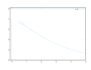
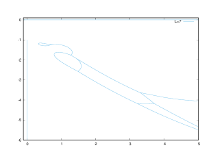
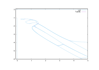
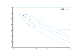
Figure 7.6: Condensation curves for partition function zeros on a $(2M+1)\times 2N$ cylinder, in the limit $N\to\infty$ (aspect ratio $\rho\to\infty$, open channel). The panels show, in reading direction, the cases $M=2,3,4,5$.

The results for the condensation curves with $M=2,3,4,5$ are shown in Figure 7.6. The curves are confined to the half-space ${\rm Im}\,u\leq 0$, and they are invariant under changing the sign of ${\rm Re}\,u$. Therefore it is enough to consider them in the fourth quadrant: ${\rm Re}\,u\geq 0$, ${\rm Im}\,u\leq 0$. The condensation curves display several noteworthy features:

1. Outside the curves and in the enclosed regions delimited by blue curves, the dominant eigenvalue belongs to the $K=M$ magnon sector (i.e., $d=1$ defect in the TL representation). For the largest size $M=5$ there are also enclosed regions delimited by green curves: in this case the dominant eigenvalue belongs to the $K=M-1$ sector ($d=3$).

2. The whole real axis forms part of the curve. In fact, when $u\in\mathbb{R}$, all the eigenvalues are equimodular and have norm $(u^{2}+1)^{M}$. Above the real axis (${\rm Im}\,u>0$) the dominant eigenvalue is the unique eigenvalue in the $K=0$ sector.

3. There is a segment of the imaginary axis, ${\rm Re}\,u=0$ and ${\rm Im}\,u\leq u_{\rm c}(M)$ which also belongs to the condensation curve. Along this segment, the two dominant eigenvalues come from the $K=M$ sector. For the end-point $u_{\rm c}(M)$ we find the following results:
   $M$ 2 3 4 5 6 7 $u_{\rm c}(M)$ -1.091487 -1.065097 -1.050552 -1.041328 -1.034954 -1.030285
   

4. It seems compelling from these data that

   $$u_{\rm c}(M)\to-1\mbox{ as }M\to\infty\,,$$ (7.19)

   with a finite-size correction proportional to $1/M$. We also note that at this asymptotic end-point, $u=-i$, for all finite $M$ there is a unique dominant eigenvalue which belongs to the $K=M$ sector and has norm 1, while all other eigenvalues have norm 0.

5. The remainder of the condensation curve forms a single connected component with no end-points. It however has a number of T-points that grows fast with $M$. Notice that we have taken great care to determine all of these T-points, some of which are very close and thus hard to distinguish in the figures. To help the reader identifying them, they have been marked by small crosses.

6. For the leftmost point $u_{\star}$ of this connected component (i.e., the point with the smallest imaginary part) we find the following results:
   $M$ 2 3 4 5 6 7 ${\rm Re}\,u_{\star}(M)$ 0.496489 0.338134 0.258384 0.209593 0.176490 0.152498 ${\rm Im}\,u_{\star}(M)$ -1.307913 -1.196739 -1.146652 -1.117510 -1.098264 -1.084539
   

7. It seems compelling from these data that

   $${\rm Re}\,u_{\star}(M)\to 0\mbox{ as }M\to\infty\,,$$

   $${\rm Im}\,u_{\star}(M)\to-1\mbox{ as }M\to\infty\,,$$ (7.20)

   both with finite-size corrections proportional to $1/M$. We conclude that the leftmost point of the connected component converges to the same value as the end-point, namely $u=-i$. This kind of “pinching” is characteristic of a phase transition [34, 35]; note however that the limit $u\to-i$ of the XXX model is singular and does not present a critical point in the usual sense.

We now compare the condensation curves with the partition function zeros. The partition functions $Z(u,M,N)$ were first computed from the algebro-geometric approach, for $M=2,3,4,5$ and $N=1024$, which corresponds to a very large aspect ratio $\rho\sim 10^{3}$. The zeros of $Z(u,M,N)$ were then computed by the program MPSolve [46][47], which is a multiprecision implementation of the Ehrlich-Aberth method [48, 49], an iterative approach to finding all zeros of a polynomial simultaneously.

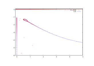
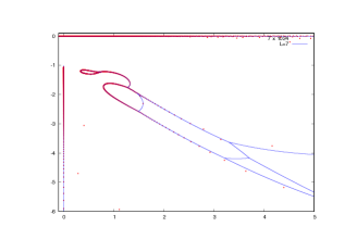
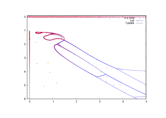
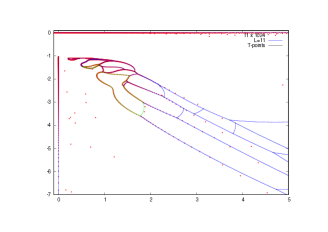
Figure 7.7: Comparison between the partition function zeros on a $(2M+1)\times 2N$ cylinder, with $N=1024$, and the corresponding condensation curves in the $N\to\infty$ limit (open channel). The panels show, in reading direction, the cases $M=2,3,4,5$.

The resulting zeros are shown in Figure 7.7, as red points superposed on the condensation curves of Figure 7.6. The agreement is in general very good, although some portions of the condensation curves are very sparsely populated with zeros; in those cases the zeros are still at a discernible distance from the curves, in spite of the large aspect ratio. We have verified that the agreement improves upon increasing $\rho$.

7.3 Closed channel

In the closed channel the $\check{R}$-matrix can be inferred from (2.15) and (2.2). It reads

$$\check{R}^{\rm c}(u)=\left(\begin{array}[]{cccc}b(u)&0&0&0\\ 0&c(u)&a(u)&0\\ 0&a(u)&c(u)&0\\ 0&0&0&b(u)\\ \end{array}\right)\,,$$ (7.25)

still with $a(u)=u+i$, $b(u)=u$ and $c(u)=i$. However, as we shall soon see, it is convenient to apply a diagonal gauge transformation $D={\rm diag}(1,-1)$ in the left in-space and the right out-space of $\check{R}^{\rm c}$; that is, $\check{R}_{12}^{\rm c}\mapsto D_{1}\,\check{R}_{12}^{\rm c}\,D_{1}$. This has the effect of changing the sign of $c(u)$ while leaving the partition function unchanged: the gauge matrices square to the identity at the intersections between $\check{R}$-matrices when taking powers of the transfer matrix $\tilde{\mathrm{t}}_{D}(u)$ given by (2.18). To complete the transformation, the first and last row of gauge transformations have to be absorbed into a redefinition of the boundary states $\langle\Psi_{0}|$ and $|\Psi_{0}\rangle$ appearing in (2.16).

7.3.1 Temperley-Lieb algebra

As in the open channel, we can rewrite the $\check{R}$-matrix in terms of TL generators (7.12):

$$\check{R}^{\rm c}_{i,i+1}(u)=\alpha I+\beta E_{i}\,.$$ (7.26)

To match (7.25), with $c(u)=-i$ after the gauge transformation, we must now set

$$\alpha=u\,,\qquad\beta=u+i\,,\qquad q=-1\,,\qquad\delta=-2\,.$$ (7.27)

In the closed channel, the TL algebra is defined on $L=2N$ sites. The goal is now to find a representation having the same dimension ${\cal N}(N)$, see (4.60), as the number of physical solutions appearing in the closed-channel expressions of the partition function, (4.2) and (4.3). This issue is more complicated than in the open channel.

As a first step, we let the TL generators act on the basis of link patterns, as before. Since the boundary states restrict to zero total spin, the only allowed number of Bethe roots is $K=N$ (see section 4). This implies that the link patterns are free of defects ($d=0$). The transfer matrix $\tilde{\mathrm{t}}_{D}(u)$ is then given by (2.18) with (7.26), where the TL generators $E_{i}$ act on the link patterns as described in section 7.2.1. To reproduce the partition function (2.16) we also need to interpret the boundary state (2.19) within the TL representation. The natural object is the quantum-group singlet of two neighboring sites

$$|\psi_{0}\rangle_{\rm TL}=q^{1/2}|\uparrow\rangle\otimes|\downarrow\rangle+q^{-1/2}|\downarrow\rangle\otimes|\uparrow\rangle\,,$$ (7.28)

which is represented in terms of link patterns as a short arc joining the neighboring sites. We should however remember at this stage the gauge transformation that allowed us to switch the sign of $c(u)$. To compensate this, we need to insert a minus sign for a down-spin in the second tensorand, to obtain

$$|\tilde{\psi}_{0}\rangle_{\rm TL}=-q^{1/2}|\uparrow\rangle\otimes|\downarrow\rangle+q^{-1/2}|\downarrow\rangle\otimes|\uparrow\rangle\,,$$ (7.29)

With $q=-1$, this is proportional to $|\psi_{0}\rangle$ of (2.19).

On the other hand it is easy to check from (7.12) that the TL generator $E_{i}$ is nothing but the (unnormalized) projector onto the quantum-group singlet. Therefore, just as $E_{i}=\raisebox{-1.00006pt}{ \leavevmode\hbox to9.34pt{\vbox to9.34pt{\text{[drawing]}}}}$, the initial boundary state $|\Psi_{0}\rangle$ can be represented graphically by the defect-free link pattern in which sites $2j-1$ and $2j$ are connected by an arc, for each $j=1,2,\ldots,N$. Similarly, the final boundary state $\langle\Psi_{0}|$ is interpreted as the TL contraction of the corresponding pairs of sites. With these identifications, we have explicitly verified for small $N$ and $M$ that the TL formalism produces the correct partition functions, such as (2.10).

With the spin-zero constraint imposed, the TL dimension is thus equal to the number of defect-free link patterns on $L=2N$ sites. This is easily shown to be given by the Catalan numbers

$${\rm Cat}(N)=\frac{1}{N+1}{2N\choose N}\,,$$ (7.30)

for which the first 10 values are given by

$$\{1,2,5,14,42,132,429,1430,4862,16796\}\,.$$ (7.31)

Although this is smaller than the dimension of the 6-vertex-model representation constrained to the $S^{z}=0$ sector, viz. ${2N\choose N}$, it is not as small as (4.60), so further work is needed.

The transfer matrix and the boundary states are also symmetric under cyclic shifts (in units of two lattice spacings) of the $L=2N$ sites. This symmetry can be used to further reduce the dimension of the transfer matrix. Indeed, after acting with $\tilde{\mathrm{t}}_{D}(u)$ we project each link pattern obtained onto a suitably chosen image under the cyclic group $\mathbb{Z}_{N}$. In this way each orbit under $\mathbb{Z}_{N}$ is mapped onto a unique representative link pattern. The dimension of the corresponding rotation invariant transfer matrix then reduces to [50]

$${\rm dim}_{\mathbb{Z}_{N}}(N)=\frac{1}{N}\sum_{m|N}\varphi(N/m){2m\choose m}-{\rm Cat}(N)\,,$$ (7.32)

where the sum is over the divisors of $N$, and $\varphi(x)$ denotes the Euler totient function. The first 10 values are given by

$$\{1,2,3,6,10,28,63,190,546,1708\}\,.$$ (7.33)

But one can go a bit further, since the transfer matrix and boundary states are also invariant under reflections. This gives rise to a symmetry under the dihedral group $\mathbb{D}_{N}$. The dimension of the rotation-and-reflection invariant transfer matrix then becomes [50]

$${\rm dim}_{\mathbb{D}_{N}}(N)=\frac{1}{2}\left(\frac{1}{N}\sum_{m|N}\varphi(N/m){2m\choose m}-{\rm Cat}(N)+{N\choose\lfloor N/2\rfloor}\right)\,,$$ (7.34)

of which the first 10 values are

$$\{1,2,3,6,10,24,49,130,336,980\}\,.$$ (7.35)

The process of imposing more and more symmetries and reducing the dimension of the relevant transfer matrices might be realized at the ZRC level by imposing more and more constraints on the $Q$-functions. Consider the ZRC of a closed spin chain with length $L=2N$ and $N$ magnons. The corresponding Bethe states are in the $S^{z}=0$ sector. In order to restrict to the parity symmetric solutions, we need to impose the condition $Q(u)=Q(-u)$ for any $u$. This leads to further constraints to the ZRC and reduces the number of allowed solutions down to $\mathcal{N}(N)$. Since $Q(u)$ is a polynomial of order $N$, the constraint $Q(u)=Q(-u)$ can also be imposed by $Q(x_{k})=Q(-x_{k})$ at $N$ different values. Now the main observation is that at certain values of $x_{k}$, the constraints have a clear physical meaning. For example, taking $x_{1}=i/2$, the constraint $Q(i/2)=Q(-i/2)$ is equivalent to

$$\frac{Q(-i/2)}{Q(+i/2)}=\prod_{k=1}^{N}\frac{u_{k}+\tfrac{i}{2}}{u_{k}-\tfrac{i}{2}}=1,$$ (7.36)

which restricts to the solutions with zero total momentum. It is therefore an interesting question to see whether the dihedral symmetry can be realized in this way. If so, at which further value(s) of $x_{k}$ would we need to impose $Q(x_{k})=Q(-x_{k})$ ?

We do not presently know if and how one can identify a TL representation whose dimension equals ${\cal N}(N)={N\choose\lfloor N/2\rfloor}$ given by (4.60). It certainly appears remarkable at this stage that

$$2\,{\rm dim}_{\mathbb{D}_{N}}(N)-{\rm dim}_{\mathbb{Z}_{N}}(N)={\cal N}(N)\,,$$ (7.37)

as already noticed in [50]. It is also worth pointing out that ${\cal N}(N)$ can be interpreted as the number of defect-free link patterns on $2N$ sites which are symmetric around the mid-point. We leave the further investigation of this question for future work.

7.3.2 Results

We have computed the condensation curves in the closed channel, using the TL link-pattern representations identified above, namely using: 1) spin-zero (i.e., defect free) link patterns, 2) spin-zero link patterns with cyclic symmetry $\mathbb{Z}_{N}$, and 3) spin-zero link patterns with dihedral symmetry.

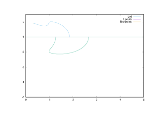
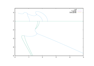
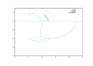
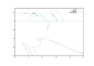
Figure 7.8: Condensation curves for partition function zeros on a $(2M+1)\times 2N$ cylinder, in the limit $M\to\infty$ (closed channel), for a system exhibiting only spin-zero symmetry. The panels show, in reading direction, the cases $N=3,4,5,6$.

Figure 7.8 shows the results using only the spin-zero constraint. In the regions enclosed by curves of blue color there is a unique dominant eigenvalue, whereas in the regions enclosed by green (resp. yellow) color the dominant eigenvalue has multiplicity two (resp. three). Obviously the sought-after representation of dimension ${\cal N}(N)$ is expected to be multiplicity-free, so the corresponding condensation curve should be free of green and yellow branches. Nevertheless, the curves in Figure 7.8 are expected to correctly produce the condensation curves of partition function zeros for any system described by the transfer matrix $\tilde{\mathrm{t}}_{D}(u)$ and with boundary states that impose only the spin-zero symmetry, while breaking any other symmetry (e.g., by imposing spatially inhomogeneous weights).

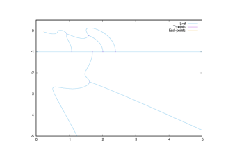
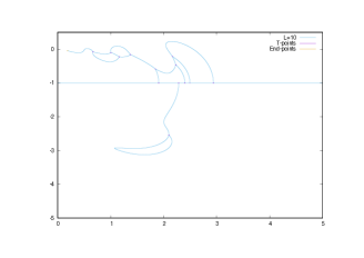
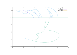
Figure 7.9: Condensation curves for partition function zeros on a $(2M+1)\times 2N$ cylinder, in the limit $M\to\infty$ (closed channel), for a system exhibiting spin-zero and cyclic symmetry $\mathbb{Z}_{N}$. The panels show, in reading direction, the cases $N=4,5,6,7$.

Next we show in Figure 7.9 the results using both the spin-zero and the cyclic symmetry $\mathbb{Z}_{N}$. When compared to Figure 7.8 it can be seen that many branches of the curves are unchanged. However all of the yellow and some of the green curves have now disappeared, reflecting the fact that the eigenvalues which were formerly dominant inside the regions enclosed by green and yellow colors have now been eliminated from the spectrum, since they do not correspond to $\mathbb{Z}_{N}$ symmetric eigenstates. The curves in Figure 7.9 should give the correct condensation curves for systems having the spin-zero and cyclic symmetries. But those with $N=4,5$ should even provide the correct results for the full “Cooper-pair” symmetry (4.35), since the TL dimension is then equal to the number of physical solutions.

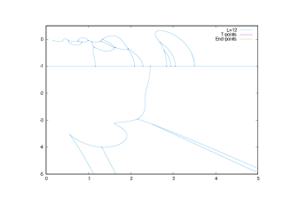
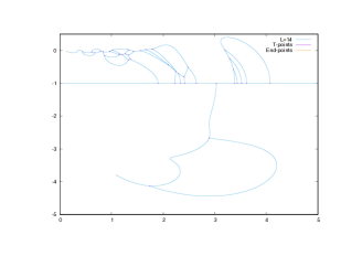
Figure 7.10: Condensation curves for partition function zeros on a $(2M+1)\times 2N$ cylinder, in the limit $M\to\infty$ (closed channel), for a system exhibiting spin-zero and dihedral symmetry $\mathbb{D}_{N}$. The panels show the cases $N=6,7$.

Finally we depict in Figure 7.10 results using the spin-zero and dihedral symmetry $\mathbb{D}_{N}$. For $N=6$ the condensation curve is identical to the one found with cyclic symmetry, meaning that none of the four eliminated eigenvalues (when going from ${\rm dim}_{\mathbb{Z}_{N}}(6)=28$ to ${\rm dim}_{\mathbb{D}_{N}}(6)=24$) was dominant anywhere in the complex $u$-plane. It should provide the correct result for the full “Cooper-pair” symmetry (4.35) if the elimination of four more eigenvalues (going from ${\rm dim}_{\mathbb{D}_{N}}(6)=24$ to ${\cal N}(6)=20$) turned out to be equally innocuous. The $N=7$ curve with dihedral symmetry has only branches corresponding to multiplicity-free eigenvalues, so it may also apply to the full paired symmetry, although a greater amount of eigenvalues are redundant in this case.

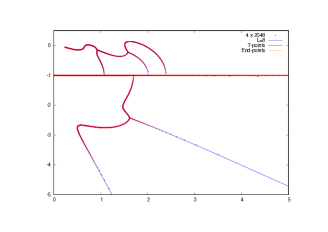
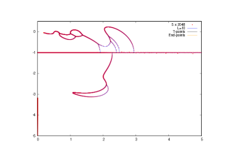
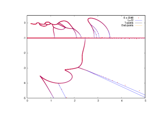
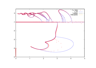
Figure 7.11: Comparison between the partition function zeros on a $(2M+1)\times 2N$ cylinder, with $M=2048$, and the corresponding condensation curves in the $M\to\infty$ limit (closed channel). The panels show, in reading direction, the cases $N=4,5,6,7$.

All the curves contain an end-point $u_{\rm e}$ close to the origin for which we have found the following results:
$N$ 4 5 6 7 8 9 ${\rm Re}\,u_{\rm e}(N)$ 0.234690 0.186435 0.154775 0.132364 0.115649 0.102696 ${\rm Im}\,u_{\rm e}(N)$ -0.057271 -0.045012 -0.037154 -0.031665 -0.027604 -0.024475
It seems compelling from these data that

$$u_{\rm e}(N)\to 0\mbox{ as }N\to\infty\,,$$ (7.38)

with finite-size correction in both the real and imaginary parts proportional to $1/N$.

To finish this section, we now compare the condensation curves with the actual partition function zeros. This is done for $N=4,5,6,7$ in Figure 7.11. For the partition function zeros, we have $M=2048$, except for $N=7$ where we have only $M=1024$; this ensures an aspect ratio $\rho<10^{-2}$ in all cases. The agreement with the condensation curves appears excellent, with the possible exception of the bubble-shaped region with $-5<{\rm Im}\,u<-2$ in the $N=7$ case.

8 Conclusions and discussions

We have computed the exact partition functions for the 6-vertex model on intermediate size lattices with periodic boundary condition in one direction and free open boundary conditions in the other. This work is a natural continuation of a previous work [7] by three of the authors on the partition function of the 6-vertex model where periodic boundary conditions were imposed in both directions. The presence of free open boundary conditions brings new features and challenges. To overcome these challenges, we have further developed the application of algebro-geometric methods to the Bethe ansatz equations in various directions. We have incorporated recent developments in integrability such as rational $Q$-systems for open spin chains [18] and the exact formulae for overlaps between integrable boundary states and Bethe states [23, 24, 25, 26, 27]. We have also developed powerful algorithms to perform the algebraic geometry computations, such as the construction of Gröbner bases and companion matrices, in the presence of a free parameter.

Equipped with these new developments, we obtained the following exact results for the cylinder partition function $Z(u,M,N)$.

• Open channel. In the open channel, for $M=1$, we obtained a closed-form expression (6.3) valid for any $N$. For $M=2,3,4,5,6$, we have computed the partition function for fixed $N$, both for small values and large values. For small values, we computed $N=2,3,4,5,6$. These results are given in appendix F. For large values, we computed $N=128,256,512,1024,2048$. These results were used to generate the zeros of partition functions in the partial thermodynamic limit. The exact results for large $N$ are not suitable to be put in the paper, so we have uploaded them as ancillary data files.

• Closed channel. In the closed channel, for $N=1,2,3$, we obtained closed-form expressions valid for any $M$. The results are given in (6.6), (6.8) and (6.26), respectively. For $N=4,5,6,7$ we have computed partition functions for fixed $M$, both for small and large values. For small values of $M$, we computed $M=2,3,4,5,6$ for $N=4,5,6$ because for these values we can compare the results in both channels and make non-trivial consistency checks. For large values of $M$, we computed $M=128,256,512,1024,2048$ for $M=4,5,6$ and $M=128,256,512,1024$ for $M=7$. The results for large values of $M$ have been used to obtain the zeros of the partition function in the closed channel and are uploaded as ancillary files.

We studied the partial thermodynamic limit of the partition function in both channels using the exact results. In particular, we computed the zeros of the partition functions in these limits and found that they condense on certain curves. The condensation curves in the partial thermodynamic limit can be found by a numerical approach based on the BKW theorem. This numerical approach has been applied in the torus case and was further developed in the current context by taking into account the new features, especially in the closed channel. Comparing the distribution of the zeros obtained from the exact partition function and the condensation curve obtained from the numerical approach, we found nice agreement and were able to shed light on several interesting features. The condensation curves in both the open and closed channels were found to involve very intricate features with multiple bifurcation points and enclosed regions. We believe that the further study of these curves might be of independent interest.

There are many other questions which deserve further investigation.

One of the most interesting directions is to compute the partition function for the $q$-deformed case. For generic values of $q$ (namely, when $q$ is not a root of unity), $Q$-systems for both closed and open chains have been formulated in a recent work [18]. This should provide a good starting point for developing an algebro-geometric approach, since $QQ$-relations are more efficient than Bethe equations and give only physical solutions. It would presumably be easier to first study the torus case where the relevant Bethe equations are those of the periodic XXZ spin chain. After that, one could move to the more complicated cylinder case.

We have focused here on the cylinder geometry with free boundary conditions. The case of fixed boundary conditions (with two arbitrary boundary parameters) may now also be in reach, using the new $Q$-system [51].

From the perspective of algebro-geometric computations, it will be desirable to sharpen the computational power of our method. For instance, we will try to apply the modern implements of Faugère’s F4 algorithm [53], which is in general more efficient than Buchberger’s algorithm.

Appendix A Basic notions of computational algebraic geometry

In this appendix, we give a brief introduction to some basic notions of computational algebraic geometry which are used in the main text.

A.1 Polynomial ring and ideal

Polynomial ring

Let us start with the notion of polynomial ring which is denoted by $A_{K}[z_{1},\ldots,z_{n}]$ or $A_{K}$ for short. It is the set of all polynomials in $n$ variables $z_{1},z_{2},\ldots,z_{n}$ whose coefficients are in the field $K$. In our case, the field is often taken to be the set of complex numbers $\mathbb{C}$ or rational numbers $\mathbb{Q}$.

Ideal

An ideal $I$ of $A_{K}$ is a subset of $A_{K}$ such that

1. $f_{1}+f_{2}\in I$, if $f_{1}\in I$ and $f_{2}\in I$,

2. $gf\in I$, for $f\in I$ and $g\in A_{K}$.

Importantly, any ideal $I$ of the polynomial ring $A_{K}$ is finitely generated. This means, for any ideal $I$, there exists a finite number of polynomials $f_{i}\in I$ such that any polynomial $F\in I$ can be written as

$$F=\sum_{i=1}^{k}f_{i}g_{i},\qquad g_{i}\in A_{K}.$$ (A.1)

We can write $I=\langle f_{1},f_{2},\ldots,f_{k}\rangle$. Here the polynomials $\{f_{k}\}$ are called a basis of the ideal.

A.2 Gröbner basis

As mentioned before, an ideal is generated by a set of basis $\{f_{1},\ldots,f_{k}\}$. The choice of the basis is not unique. Namely, the same ideal can be generated by several different choices of bases

$$I=\langle f_{1},\ldots,f_{k}\rangle=\ldots=\langle g_{1},\ldots,g_{s}\rangle.$$ (A.2)

Notice that in general $k$ does not have to be the same as $s$. For many cases, a convenient basis is needed. For solving polynomial equations and the polynomial reduction problem, it is most convenient to work with a Gröbner basis.

We can introduce the Gröbner basis by considering polynomial reduction. A polynomial reduction of a given polynomial $F$ over a set of polynomials $\{f_{1},\ldots,f_{k}\}$ is given by

$$F=\sum g_{i}f_{i}+r,\qquad g_{i}\in A_{K}$$ (A.3)

where $r$ is a polynomial that cannot be reduced further by any of the $f_{i}$. The polynomial $r$ is called the remainder of the polynomial reduction. One important fact is that the polynomial reduction is not unique for a generic basis $\{f_{1},\ldots,f_{k}\}$. As a simple example, let us take $f_{1}=y^{2}-1$ and $f_{2}=xy-1$, and consider $F(x,y)=x^{2}y+xy^{2}+y^{2}$. The polynomial reduction of $F(x,y)$ over $f_{1}$ and $f_{2}$ can be performed in two different ways

$$F(x,y)= \,(x+1)\,f_{1}+x\,f_{2}+(2x+1),$$ (A.4)

$$F(x,y)= \,f_{1}+(x+y)f_{2}+(x+y+1).$$

As we can see, the remainders are $r_{1}=2x+1$ and $r_{2}=x+y+1$ respectively. Therefore for a generic basis, the remainder of the polynomial is not well-defined. A basis of an ideal $\{g_{1},\ldots,g_{s}\}$ is said to be a Gröbner basis if the polynomial reduction is well-defined in the sense that the remainder is unique. Now we move to the more formal definition of the Gröbner basis.

Monomial ordering

To define a Gröbner basis, we first need to define monomial orders in the polynomial ring. A monomial order $\prec$ is specified by the following two rules

• If $u\prec v$ then for any monomial $w$, we have $uw\prec vw$.

• If $u$ is non-constant monomial, then $1\prec u$.

Some commonly used orders are lex (Lexicographic), deglex (DegreeLexicographic) and degrevlex (DegreeReversedLexicographic).

Leading term

Once a monomial order $\prec$ is specified, for any polynomial $f$, we can define the leading term uniquely. The leading term, which is denoted by LT($f$), is defined as the highest monomial of $f$ with respect to the monomial order $\prec$.

Gröbner basis

A Gröbner basis $G(I)$ of an ideal $I$ with respect to the monomial order $\prec$ is a basis of the ideal $\{g_{1},\ldots,g_{s}\}$ such that for any $f\in I$, there exists a $g_{i}\in G(I)$ such that LT($f$) is divisible by LT($g_{i}$). A Gröbner basis for a given ideal with a monomial order can by computed by standard algorithms such as Buchberger algorithm [52] or the F4/F5 algorithms [53]. For an ideal $I$, given a monomial order $\prec$, the so-called minimal reduced Gröbner basis is unique.

A.3 Quotient ring and companion matrix

Quotient ring

Given an ideal $I$, we can define the quotient ring $A_{K}/I$ by the equivalence relation: $f\sim g$ if and only if $f-g\in I$.

Polynomial reduction and Gröbner basis provide a canonical representation of the elements in the quotient ring $A_{K}/I$. Two polynomials $F_{1}$ and $F_{2}$ belong to the same element in the quotient ring $A_{K}/I$ if and only if their remainders of the polynomial reduction are the same. In particular, $f\in I$ if and only if its remainder of the polynomial reduction is zero. This gives a very efficient method to determine whether a polynomial $f$ is in the ideal $I$ or not.

Dimension of quotient ring

To our purpose, the dimension of the quotient ring is important. Consider a system of polynomial equations of $n$ variables

$$f_{1}(z_{1},\ldots,z_{n})=\cdots=f_{k}(z_{1},\ldots,z_{n})=0,$$ (A.5)

we can define the ideal and the quotient ring as

$$I=\langle f_{1},\ldots,f_{k}\rangle,\qquad Q_{I}=\mathbb{C}[z_{1},\ldots,z_{n}]/\langle f_{1},\ldots,f_{k}\rangle.$$ (A.6)

One crucial result is that the linear dimension of the quotient ring $\text{dim}_{K}Q_{I}$ equals the number of the solutions of the system (A.5). Therefore, if the number of solutions of the polynomial equations (A.5) is finite, $Q_{I}$ is a finite dimensional linear space. Let $G(I)$ be the Gröbner basis of the ideal $I$. The linear space is spanned by monomials which are not divisible by any elements in LT[$G(I)$].

Companion matrix

Another important notion for our applications is the companion matrix. The main idea is that we can represent any polynomial $f\in A_{K}$ as a matrix in the quotient ring which is a finite dimensional linear space. More precisely, let $(m_{1},\ldots,m_{N})$ be the monomial basis of $A_{K}/I$, which can be constructed by the Gröbner basis $G(I)$. Given any polynomial, we can define an $N\times N$ matrix as follows

1. Multiply $f$ with one of the basis monomials $m_{i}$, perform the polynomial reduction with respect to the Gröbner basis $G(I)$ and find the remainder $r_{i}$. It is clear that $r_{i}$ sits in the quotient ring $A_{K}/I$.

2. Since $r_{i}$ is in the quotient ring, we can expand it in terms of the basis $(m_{1},\ldots,m_{N})$, namely $r_{i}=c_{ij}m_{j}$. In terms of formulas, we can write

   $$[f\times m_{i}]_{G(I)}=\sum_{j}c_{ij}\,m_{j}$$ (A.7)

   where $[F]_{G(I)}$ means the remainder of the polynomial reduction of $F$ with respect to the Gröbner basis $G(I)$.

3. The companion matrix of $f$ is defined by

   $$(M_{f})_{ij}=c_{ij}.$$ (A.8)

Properties of companion matrix

Let us denote the companion matrix of the polynomials $f$ and $g$ by $M_{f}$ and $M_{g}$. It is clear that $M_{f}=M_{g}$ if and only if $[f]=[g]$ in $A_{K}/I$. Furthermore, we have the following properties

$$M_{f+g}=M_{f}+M_{g},\qquad M_{fg}=M_{f}M_{g}=M_{g}M_{f}.$$ (A.9)

If $M_{g}$ is an invertible matrix, we can actually define the companion matrix of the rational function $f/g$ by

$$M_{f/g}=M_{f}M_{g}^{-1}.$$ (A.10)

The companion matrix is a powerful tool for computing the sum over solutions of the polynomial system (A.5). As we mentioned before, the dimension of $Q_{I}$ equals the number of solutions of (A.5). Let us denote the $N$ solutions to be $(\vec{\xi}_{1},\ldots,\vec{\xi}_{N})$. Then we have the following important result

$$\sum_{i=1}^{N}f(\vec{\xi}_{i})=\text{Tr}\,M_{f}.$$ (A.11)

Appendix B More details on AG computation

In this section, we summarize the algorithm of our algebra-geometry based partition function computation for this paper.

• We first compute the Gröbner basis and quotient ring linear basis of the TQ relation equations (3.23) and QQ relation equations (4.55). Note that the TQ and QQ relations contain the free parameter $u$. It is possible to compute the corresponding Gröbner basis analytically in $u$ via sophisticated computational algebraic-geometry algorithms, like “slimgb” in the software Singular [54].

  However, we find that it is more efficient to set $u$ to some integral value, and compute the Groebner basis. The computation is done with the standard Gröbner basis command “std” in Singular. In this approach, we maximize the power of parallelization since the Groebner basis running time for different values of $u$ is quite uniform.

• Then we compute the power of companion matrices $(\mathbb{T}_{M,K})^{N}$. Although from the Gröbner basis it is straightforward to evaluate $(\mathbb{T}_{M,K})^{N}$, $\mathbb{T}_{M,K}$ is usually a dense matrix and the matrix product is a heavy computation. Instead, we postpone the matrix computations to the end, and evaluate the polynomial power $F^{N}$ first. Here $F$ is the corresponding polynomial of $\mathbb{T}_{M,K}$. After each polynomial multiplication step, we divide the polynomial by the ideal’s Gröbner basis to save RAM usage by trimming high-degree terms. To speed up the computation, we apply the binary strategy, i.e., $F^{N}=F^{N/2}F^{N/2}$. After $F^{N}$ is calculated, a standard polynomial division computation provides the companion matrix power $(\mathbb{T}_{M,K})^{N}$. So the partition function for a particular $u$ value is obtained.

• In previous steps, $u$ is set as an integral number. To get the analytic partition function in $u$, we have to repeat the computation, and then interpolate in $u$. We know that for both the closed and open channel partition functions, the maximum degree in $u$ is $2MN$. Hence, we compute the partition function with $2MN+1$ integer values. These results are then interpolated to the analytic partition function in $u$. The interpolation is carried out with the Newton polynomial method.

The whole computation is powered by our codes in Singular. The parallelization is implemented in the Gröbner basis and companion matrix power steps, for different integer values of $u$’s. The interpolation step is not parallelized, although it is also straightforward to do so in the future.

We remark that through the computations, the coefficient field is chosen to be the rational number field $\mathbb{Q}$. We observe that the resulting analytic partition function contains large-integer coefficients, so finite-field techniques may not speed up the computation.

Appendix C The overlap (4.36)

The overlap (4.36) can be deduced from results in the paper by Pozsgay and Rákos [27] (based on [23, 24]), to which we refer here by PR. Their $R$-matrix is given by PR (2.6), which has the same form as ours (2.7), except with

$$a(u)=\sinh(u+\eta)\,,\qquad b(u)=\sinh(u)\,,\qquad c(u)=\sinh(\eta)\,.$$ (C.1)

Moreover, they work with the “quantum monodromy matrix” given by PR (2.33)

$$T_{QTM}(u) =R_{2N,0}(u-\eta+\omega)\,R_{2N-1,0}(u-\omega)\,\ldots R_{2,0}(u-\eta+\omega)\,R_{1,0}(u-\omega)$$

$$=\left(\begin{array}[]{cc}A(u)&B(u)\\ C(u)&D(u)\\ \end{array}\right)\,.$$ (C.4)

By choosing

$$\omega=\frac{\eta}{2}-u\,,$$ (C.5)

scaling the variables as

$$u\mapsto\epsilon\,u\,,\qquad\eta\mapsto i\epsilon\,,$$ (C.6)

and keeping the leading order in $\epsilon$, our shifted monodromy matrix $\widehat{T}_{a}^{(2N)}(u-\frac{i}{2};\{\theta_{j}(u)\})$ (3.2) with alternating inhomogeneities (4.21) can be obtained.

In order to relate the generic boundary states PR (2.36)–(2.38) to the dimer state, the boundary parameters in PR (2.15) can be chosen as follows

$$\alpha\rightarrow\infty\,,\qquad\beta=0\,,\qquad\theta=0\,,$$ (C.7)

so that the K-matrices are proportional to the identity matrix. In this limit, the overlap PR (3.4) together with PR (3.3) gives our overlap (4.36).

Appendix D The relation (4.40)

We show here that the relation (4.40) follows from two simpler lemmata.

Lemma 1:

$$\langle\Phi_{0}|U^{\dagger}=\left(\frac{i}{2v-i}\right)^{N}\langle\Phi_{0}|\tau(v;\{\theta_{j}(v)\})\,.$$ (D.1)

This lemma follows from the observation

$$\tau(v;\{\theta_{j}(v)\})=i^{N}R_{12}(2v)\,R_{34}(2v)\ldots R_{2N-1,2N}(2v)\,P_{2N-3,2N-1}\,\ldots P_{3,5}\,P_{1,3}\,,$$ (D.2)

together with

$$\langle\Phi_{0}|R_{12}(2v)\,R_{34}(2v)\ldots R_{2N-1,2N}(2v)=(2v-i)^{N}\langle\Phi_{0}|\,,$$ (D.3)

and

$$\langle\Phi_{0}|P_{2N-3,2N-1}\,\ldots P_{3,5}\,P_{1,3}=(-1)^{N}\langle\Phi_{0}|U^{\dagger}\,.$$ (D.4)

Taking the scalar product of (D.1) with transfer-matrix eigenvectors $|\mathbf{u}\rangle$ (which are constructed using B-operators with alternating inhomogeneities $\{\theta_{j}(v)\}$) and setting $v=\frac{\tilde{u}}{2}$, we obtain

$$\langle\Phi_{0}|U^{\dagger}|\mathbf{u}\rangle =\left(\frac{i}{\tilde{u}-i}\right)^{N}\langle\Phi_{0}|\tau(\tfrac{\tilde{u}}{2};\{\theta_{j}(\tfrac{\tilde{u}}{2})\})|\mathbf{u}\rangle$$

$$=\left(\frac{i}{\tilde{u}-i}\right)^{N}\Lambda_{\rm c}(\tfrac{\tilde{u}}{2};\{\theta_{j}(\tfrac{\tilde{u}}{2})\})\langle\Phi_{0}|\mathbf{u}\rangle\,.$$ (D.5)

Lemma 2:

The following relation is valid off shell

$$\langle\Phi_{0}|\mathbf{u}\rangle=\left(\frac{2v-i}{2v+i}\right)^{N}\langle\mathbf{u}|\Phi_{0}\rangle\,.$$ (D.6)

See e.g. (3.3) in [27], with (C.5) and (C.6).

For our case, with $v=\frac{\tilde{u}}{2}$, we have

$$\langle\Phi_{0}|\mathbf{u}\rangle=\left(\frac{\tilde{u}-i}{\tilde{u}+i}\right)^{N}\langle\mathbf{u}|\Phi_{0}\rangle\,.$$ (D.7)

Inserting (D.7) in the RHS of (D.5), we obtain

$$\langle\Phi_{0}|U^{\dagger}|\mathbf{u}\rangle=\left(\frac{i}{\tilde{u}+i}\right)^{N}\Lambda_{\rm c}(\tfrac{\tilde{u}}{2};\{\theta_{j}(\tfrac{\tilde{u}}{2})\})\langle\mathbf{u}|\Phi_{0}\rangle\,,$$ (D.8)

which coincides with (4.40).

Appendix E Parity of states with paired Bethe roots

Following [55, 56], the parity operator $\Pi$ in the closed channel (length $2N$) is defined by

$$\Pi\,X_{n}\,\Pi^{-1}=X_{2N+1-n}\,,$$ (E.1)

where $X_{n}$ is any operator at site $n\in\{1,2,\ldots,2N\}$, and is given by

$$\Pi=P_{1,2N}\,P_{2,2N-1}\ldots P_{N,N+1}\,,$$ (E.2)

hence $\Pi=\Pi^{-1}=\Pi^{{\dagger}}$. The parity operator has a simple and beautiful action on the $B$-operator, namely

$$\Pi\,B(u)\,\Pi=-B(-u)\,,$$ (E.3)

while the reference state (4.15) remains invariant under parity

$$\Pi\,|0\rangle=|0\rangle\,.$$ (E.4)

It follows from (E.3) and (E.4) that Bethe states (4.16) corresponding to the paired Bethe roots (4.35) (even $N$) are eigenstates of parity with eigenvalue $+1$

$$\Pi|u_{1}\,,-u_{1}\,,\ldots\,,u_{\frac{N}{2}}\,,-u_{\frac{N}{2}}\rangle=|u_{1}\,,-u_{1}\,,\ldots\,,u_{\frac{N}{2}}\,,-u_{\frac{N}{2}}\rangle\,.$$ (E.5)

Similarly, Bethe states corresponding to the paired Bethe roots (4.42) (odd $N$) are eigenstates of parity with eigenvalue $-1$

$$\Pi|u_{1}\,,-u_{1}\,,\ldots\,,u_{\frac{N-1}{2}}\,,-u_{\frac{N-1}{2}}\,,0\rangle=-|u_{1}\,,-u_{1}\,,\ldots\,,u_{\frac{N-1}{2}}\,,-u_{\frac{N-1}{2}}\,,0\rangle\,.$$ (E.6)

The dimer state $|\Phi_{0}\rangle$ (4.25) is an eigenstate of parity with eigenvalue $(-1)^{N}$

$$\Pi|\Phi_{0}\rangle=(-1)^{N}|\Phi_{0}\rangle\,,$$ (E.7)

which is consistent with the fact that the overlaps $\langle\Phi_{0}|\mathbf{u}\rangle$ are nonzero only for Bethe states with paired Bethe roots (4.35), (4.42).

Appendix F Exact partition functions

In this appendix, we list all the exact partition functions for $2\leq M,N\leq 6$ apart from the simple ones that have already been given in the main text (2.10). For these values of $M$ and $N$, the partition function can be computed in both channels. As a consistency check, computations in the two channels give the same result, as it should be.

F.1 $N=6$

$$Z_{6,6}= \,2u^{72}+288iu^{71}-14328u^{70}-414000iu^{69}+8317584u^{68}+127125504iu^{67}$$ (F.1)

$$\,-1559236944u^{66}-15897457728iu^{65}+138130609500u^{64}+1041934800608iu^{63}$$

$$\,-6921377423424u^{62}-40952806081344iu^{61}+217832067312960u^{60}+1049571874084608iu^{59}$$

$$\,-4610142527559840u^{58}-18559041008388480iu^{57}+68788394401561470u^{56}$$

$$\,+235662122430397008iu^{55}-748761418763439296u^{54}-2212828011779983200iu^{53}$$

$$\,+6098355792769470156u^{52}+15707717731534712832iu^{51}-37888459151633760240u^{50}$$

$$\,-85733900199121648320iu^{49}+182272478003908656432u^{48}+364591770627856882608iu^{47}$$

$$\,-686967220132168504248u^{46}-1220600244357970313168iu^{45}+2047050659153089585764u^{44}$$

$$\,+3243098453976454684320iu^{43}-4857133424214480178560u^{42}-6881082470938635503328iu^{41}$$

$$\,+9226096556900912648334u^{40}+11712585761982875838624iu^{39}-14083587268444001339280u^{38}$$

$$-16044127855808638420656iu^{37}+17319816398521272862676u^{36}+17719150885149621701664iu^{35}$$

$$\,-17180252444447853950520u^{34}-15786443250650483906112iu^{33}+13745313212235461309790u^{32}$$

$$\,+11338458117413798884752iu^{31}-8858516711168371303152u^{30}-6552673143433555176576iu^{29}$$

$$\,+4587036228059022522828u^{28}+3037167694581592157600iu^{27}-1900876723794459666576u^{26}$$

$$\,-1123749410112064351008iu^{25}+626974446577452175698u^{24}+329820882193355585184iu^{23}$$

$$\,-163410941489958322920u^{22}-76159342969170112944iu^{21}+33342588484553082888u^{20}$$

$$\,+13690734769961746560iu^{19}-5263022902673709824u^{18}-1890408224237932800iu^{17}$$

$$\,+633003570392541120u^{16}+197095658448168960iu^{15}-56899838812276224u^{14}$$

$$\,-15180285240013824iu^{13}+3728675863226880u^{12}+839585772859392iu^{11}$$

$$\,-172442609104896u^{10}-32118023696384iu^{9}+5386833271296u^{8}$$

$$\,+806617128960iu^{7}-106666801152u^{6}-12280172544iu^{5}+1206835200u^{4}$$

$$\,+98304000iu^{3}-6340608u^{2}-294912iu+8192$$

$$Z_{5,6}= \,2u^{60}+240iu^{59}-10200u^{58}-247760iu^{57}+4106064u^{56}+50944128iu^{55}$$ (F.2)

$$\,-501290288u^{54}-4069332864iu^{53}+28034725284u^{52}+167372075712iu^{51}$$

$$-879568749504u^{50}-4117046950656iu^{49}+17320477694784u^{48}+65956540414464iu^{47}$$

$$\,-228627359471520u^{46}-724727457569280iu^{45}+2108994608155482u^{44}+5652786955676832iu^{43}$$

$$\,-13995089127459600u^{42}-32084625043816128iu^{41}+68261467147861284u^{40}$$

$$\,+135034284911783616iu^{39}-248788374633283104u^{38}-427529707088463360iu^{37}$$

$$\,+686116309138082856u^{36}+1029410431077285360iu^{35}-1445199354794151720u^{34}$$

$$\,-1899914808354007664iu^{33}+2340240191331772812u^{32}+2702070900176216160iu^{31}$$

$$\,-2925317019312145664u^{30}-2970027518108113056iu^{29}+2827960377154344960u^{28}$$

$$\,+2525039773174991216iu^{27}-2113704343901047104u^{26}-1658217850739230320iu^{25}$$

$$\,+1218539894552498448u^{24}+838213811707493088iu^{23}-539306661016030248u^{22}$$

$$\,-324234959917029984iu^{21}+181939121823624930u^{20}+95158509487089840iu^{19}$$

$$\,-46317104213610216u^{18}-20941877029818960iu^{17}+8777163928275864u^{16}$$

$$\,+3401716413897600iu^{15}-1215689053318848u^{14}-399309726257280iu^{13}+120092906906976u^{12}$$

$$\,+32925815343360iu^{11}-8187331182336u^{10}-1835366381568iu^{9}+368278769664u^{8}+65577553920iu^{7}$$

$$\,-10251309056u^{6}-1387327488iu^{5}+159490560u^{4}+15134720iu^{3}-1136640u^{2}-61440iu+2048$$

$$Z_{4,6}= \,8u^{48}+336iu^{47}-7728u^{46}-123856iu^{45}+1484064u^{44}+13860000iu^{43}$$ (F.3)

$$\,-104403144u^{42}-652530240iu^{41}+3461257458u^{40}+15858754400iu^{39}-63627652560u^{38}$$

$$\,-225943164384iu^{37}+716128871152u^{36}+2039662782720iu^{35}-5249124545904u^{34}$$

$$\,-12261248086848iu^{33}+26092620286092u^{32}+50742484822368iu^{31}-90406264918472u^{30}$$

$$\,-147877208599872iu^{29}+222439906309668u^{28}+308118607243360iu^{27}-393433500079944u^{26}$$

$$\,-463456204858080iu^{25}+503911508965434u^{24}+505852778886192iu^{23}-468842183109432u^{22}$$

$$\,-401107676795728iu^{21}+316601908242108u^{20}+230384778687264iu^{19}-154393257821456u^{18}$$

$$\,-95159659506624iu^{17}+53851823641602u^{16}+27924428347584iu^{15}-13235329354320u^{14}$$

$$\,-5716979185248iu^{13}+2242521937456u^{12}+795411629952iu^{11}-253808103360u^{10}$$

$$\,-72409421696iu^{9}+18332792928u^{8}+4082245632iu^{7}-790647936u^{6}-131353344iu^{5}+18380160u^{4}$$

$$\,+2105344iu^{3}-190464u^{2}-12288iu+512$$

$$Z_{3,6}= \,2u^{36}+144iu^{35}-3240u^{34}-41760iu^{33}+371556u^{32}+2500704iu^{31}$$ (F.4)

$$\,-13426440u^{30}-59457600iu^{29}+222050034u^{28}+710461408iu^{27}-1970740872u^{26}$$

$$\,-4783539888iu^{25}+10235477796u^{24}+19420445664iu^{23}-32825856240u^{22}-49607005056iu^{21}$$

$$\,+67208955660u^{20}+81794924496iu^{19}-89535239664u^{18}-88204716144iu^{17}+78198825096u^{16}$$

$$\,+62348094624iu^{15}-44646023160u^{14}-28655915040iu^{13}+16442440386u^{12}+8405591184iu^{11}$$

$$\,-3811764096u^{10}-1524747232iu^{9}+534186864u^{8}+162405504iu^{7}-42326208u^{6}-9318528iu^{5}$$

$$\,+1700640u^{4}+249600iu^{3}-28800u^{2}-2304iu+128$$

$$Z_{2,6}= \,2u^{24}+96iu^{23}-1488u^{22}-12464iu^{21}+67908u^{20}+267360iu^{19}$$ (F.5)

$$\,-818024u^{18}-2043648iu^{17}+4286358u^{16}+7635536iu^{15}-11600448u^{14}-15070368iu^{13}$$

$$\,+16767884u^{12}+15970080iu^{11}-12994512u^{10}-9014240iu^{9}+5311314u^{8}+2637792iu^{7}-1094360u^{6}$$

$$\,-375504iu^{5}+103512u^{4}+22016iu^{3}-3648u^{2}-384iu+32$$

F.2 $N=5$

$$Z_{6,5}= \,2u^{60}+240iu^{59}-10140u^{58}-248000iu^{57}+4185570u^{56}+53344848iu^{55}$$ (F.6)

$$\,-542357480u^{54}-4562838000iu^{53}+32597238180u^{52}+201557883000iu^{51}-1094433249708u^{50}$$

$$\,-5278042287600iu^{49}+22813265943960u^{48}+89030269264680iu^{47}-315622898284860u^{46}$$

$$\,-1021614345486960iu^{45}+3032155944987750u^{44}+8282078769490080iu^{43}-20883263266224960u^{42}$$

$$\,-48740210535148320iu^{41}+105537643218985020u^{40}+212434648891515000iu^{39}$$

$$\,-398192299717983780u^{38}-696081663569207040iu^{37}+1136284932112092120u^{36}$$

$$\,+1734011186676432768iu^{35}-2476033587009228660u^{34}-3310802034120343280iu^{33}$$

$$\,+4148085867425363430u^{32}+4871950812684428040iu^{31}-5365880829686871812u^{30}$$

$$\,-5543013568038622320iu^{29}+5370865405192114860u^{28}+4880969524493532440iu^{27}$$

$$\,-4159536448109346180u^{26}-3322896661947378912iu^{25}+2487244973239722900u^{24}$$

$$\,+1743350380048456200iu^{23}-1143361265067321060u^{22}-700989597010688640iu^{21}$$

$$\,+401316693215927490u^{20}+214260526736194800iu^{19}-106515303269030220u^{18}$$

$$\,-49218120113100480iu^{17}+21095469547685670u^{16}+8367142598539080iu^{15}-3062728016717700u^{14}$$

$$\,-1031401068624240iu^{13}+318402566218770u^{12}+89734056144240iu^{11}-22976204056848u^{10}$$

$$\,-5314648800960iu^{9}+1103026376160u^{8}+203688568320iu^{7}-33111380480u^{6}-4671793152iu^{5}$$

$$\,+561016320u^{4}+55685120iu^{3}-4362240u^{2}-245760iu+8192$$

$$Z_{5,5}= \,2u^{50}+200iu^{49}-6800u^{48}-133600iu^{47}+1816720u^{46}+18696280iu^{45}$$ (F.7)

$$\,-153516300u^{44}-1041341760iu^{43}+5980862700u^{42}+29622561920iu^{41}-128320692620u^{40}$$

$$\,-491601126800iu^{39}+1680469080490u^{38}+5162580577360iu^{37}-14337030631180u^{36}$$

$$\,-36164934863280iu^{35}+83189622229650u^{34}+175077243069600iu^{33}-338033265929600u^{32}$$

$$\,-600140879412320iu^{31}+981612780573350u^{30}+1481512519939600iu^{29}-2065877195101300u^{28}$$

$$\,-2664254653480000iu^{27}+3180146358121680u^{26}+3515139558674328iu^{25}-3599034368401500u^{24}$$

$$\,-3413530724251600iu^{23}+2998653880187200u^{22}+2438862766979800iu^{21}-1835361722793380u^{20}$$

$$\,-1276908650973200iu^{19}+820389106281650u^{18}+486066456229800iu^{17}-265119363721020u^{16}$$

$$\,-132847449311520iu^{15}+61002271510150u^{14}+25593377506000iu^{13}-9776149068460u^{12}$$

$$\,-3385803508640iu^{11}+1057993826450u^{10}+296565427400iu^{9}-74059916520u^{8}-16339593600iu^{7}$$

$$\,+3151663680u^{6}+524266240iu^{5}-73811200u^{4}-8550400iu^{3}+780800u^{2}+51200iu-2048$$

$$Z_{4,5}= \,2u^{40}+160iu^{39}-4440u^{38}-69280iu^{37}+728000u^{36}+5674392iu^{35}$$ (F.8)

$$\,-34874340u^{34}-176140320iu^{33}+752228880u^{32}+2769883720iu^{31}-8912697344u^{30}$$

$$\,-25297249440iu^{29}+63775686230u^{28}+143577146200iu^{27}-289901804220u^{26}$$

$$\,-526881584016iu^{25}+864503010900u^{24}+1283718138360iu^{23}-1728451887060u^{22}$$

$$\,-2113229980800iu^{21}+2348251006860u^{20}+2372768013000iu^{19}-2180177662980u^{18}$$

$$\,-1820882530080iu^{17}+1381238400930u^{16}+950393607264iu^{15}-592143230220u^{14}$$

$$\,-333299096320iu^{13}+168978930950u^{12}+76875351000iu^{11}-31236020084u^{10}$$

$$\,-11269764880iu^{9}+3584938290u^{8}+996761760iu^{7}-239659680u^{6}-49170048iu^{5}+8454080u^{4}$$

$$\,+1185280iu^{3}-130560u^{2}-10240iu+512$$

$$Z_{3,5}= \,2u^{30}+120iu^{29}-2340u^{28}-25120iu^{27}+182970u^{26}+1000824iu^{25}$$ (F.9)

$$\,-4342200u^{24}-15435600iu^{23}+45931380u^{22}+116188080iu^{21}-252735000u^{20}$$

$$\,-476824800iu^{19}+785325960u^{18}+1134545880iu^{17}-1442491140u^{16}-1617100080iu^{15}$$

$$\,+1599383250u^{14}+1395092760iu^{13}-1072037820u^{12}-724305120iu^{11}+428924070u^{10}$$

$$\,+221637600iu^{9}-99319260u^{8}-38260800iu^{7}+12523890u^{6}+3435384iu^{5}-774840u^{4}-139840iu^{3}$$

$$\,+19680u^{2}+1920iu-128$$

$$Z_{2,5}= \,32u^{20}+320iu^{19}-1760u^{18}-7680iu^{17}+28560u^{16}+87696iu^{15}$$ (F.10)

$$\,-218880u^{14}-446160iu^{13}+747090u^{12}+1031120iu^{11}-1177868u^{10}-1117760iu^{9}+880230u^{8}$$

$$\,+572520iu^{7}-306660u^{6}-134064iu^{5}+46290u^{4}+12240iu^{3}-2480u^{2}-320iu+32$$

F.3 $N=4$

$$Z_{6,4}= \,2u^{48}+192iu^{47}-6432u^{46}-125344iu^{45}+1695768u^{44}+17380704iu^{43}$$ (F.11)

$$\,-142071744u^{42}-957909984iu^{41}+5456197416u^{40}+26727665408iu^{39}-114171998592u^{38}$$

$$\,-430010518272iu^{37}+1440779616064u^{36}+4325994981888iu^{35}-11709940237824u^{34}$$

$$\,-28718431904256iu^{33}+64075191370944u^{32}+130502828494848iu^{31}-243315793126400u^{30}$$

$$\,-416238684174336iu^{29}+654563752915968u^{28}+947664700456960iu^{27}-1264641410790912u^{26}$$

$$\,-1556980053712896iu^{25}+1769626440158208u^{24}+1857530670661632iu^{23}-1801001830855680u^{22}$$

$$\,-1612788643440640iu^{21}+1333448855969280u^{20}+1017287720361984iu^{19}-715462372579328u^{18}$$

$$\,-463315439579136iu^{17}+275828260637184u^{16}+150674393284608iu^{15}-75348310695936u^{14}$$

$$\,-34399109013504iu^{13}+14290811226112u^{12}+5382179758080iu^{11}-1829435990016u^{10}$$

$$\,-558255153152iu^{9}+151954421760u^{8}+36599955456iu^{7}-7720648704u^{6}-1406828544iu^{5}$$

$$\,+217178112u^{4}+27590656iu^{3}-2752512u^{2}-196608iu+8192$$

$$Z_{5,4}= \,2u^{40}+160iu^{39}-4512u^{38}-72352iu^{37}+789416u^{36}+6439584iu^{35}$$ (F.12)

$$\,-41590944u^{34}-220803168iu^{33}+988466328u^{32}+3799026688iu^{31}-12701096768u^{30}$$

$$\,-37309082496iu^{29}+97056390560u^{28}+225028607488iu^{27}-467409758976u^{26}-873387327744iu^{25}$$

$$\,+1472970252384u^{24}+2247880822272iu^{23}-3110257952256u^{22}-3907451351040iu^{21}$$

$$\,+4461712923648u^{20}+4633176305664iu^{19}-4376312765952u^{18}-3759173240832iu^{17}$$

$$\,+2934531772416u^{16}+2079427166208iu^{15}-1335273784320u^{14}-775224616960iu^{13}$$

$$\,+405738771968u^{12}+190745063424iu^{11}-80192927744u^{10}-29991620608iu^{9}+9914835456u^{8}$$

$$\,+2874777600iu^{7}-723861504u^{6}-156229632iu^{5}+28375040u^{4}+4218880iu^{3}$$

$$\,-491520u^{2}-40960iu+2048$$

$$Z_{4,4}= \,2u^{32}+128iu^{31}-2720u^{30}-33088iu^{29}+275920u^{28}+1721920iu^{27}$$ (F.13)

$$\,-8468640u^{26}-33967296iu^{25}+113839344u^{24}+324510720iu^{23}-797262912u^{22}$$

$$\,-1704729984iu^{21}+3195196320u^{20}+5276663040iu^{19}-7705800576u^{18}-9976315392iu^{17}$$

$$\,+11469719520u^{16}+11721735168iu^{15}-10651210752u^{14}-8600710656iu^{13}+6162514560u^{12}$$

$$\,+3908175360iu^{11}-2185631232u^{10}-1072522752iu^{9}+458877312u^{8}+169820160iu^{7}-53830656u^{6}$$

$$\,-14436352iu^{5}+3218944u^{4}+581632iu^{3}-81920u^{2}-8192iu+512$$

$$Z_{3,4}= \,2u^{24}+96iu^{23}-1536u^{22}-13376iu^{21}+76656u^{20}+321984iu^{19}$$ (F.14)

$$\,-1060064u^{18}-2847552iu^{17}+6375696u^{16}+12024320iu^{15}-19217088u^{14}-26146944iu^{13}$$

$$\,+30396896u^{12}+30257664iu^{11}-25802112u^{10}-18824192iu^{9}+11701920u^{8}+6151680iu^{7}$$

$$\,-2706944u^{6}-984576iu^{5}+290688u^{4}+68096iu^{3}-12288u^{2}-1536iu+128$$

$$Z_{2,4}= \,2u^{16}+64iu^{15}-576u^{14}-2912iu^{13}+9928u^{12}+24864iu^{11}$$ (F.15)

$$\,-47840u^{10}-71968iu^{9}+85176u^{8}+80128iu^{7}-60608u^{6}-36480iu^{5}+16864u^{4}+5888iu^{3}$$

$$\,-1536u^{2}-256iu+32$$

F.4 $N=3$

$$Z_{6,3}= \,2u^{36}+144iu^{35}-3672u^{34}-54720iu^{33}+566172u^{32}+4421808iu^{31}$$ (F.16)

$$\,-27359952u^{30}-138421152iu^{29}+585564318u^{28}+2106246952iu^{27}-6526250244u^{26}$$

$$\,-17601308640iu^{25}+41667849936u^{24}+87178071096iu^{23}-162100318500u^{22}$$

$$\,-269073694512iu^{21}+400109679918u^{20}+534347671248iu^{19}-642039336300u^{18}$$

$$\,-694728826992iu^{17}+677171433726u^{16}+594340399176iu^{15}-469220702148u^{14}$$

$$\,-332676139248iu^{13}+211359220146u^{12}+119998562832iu^{11}-60673432464u^{10}$$

$$\,-27204293440iu^{9}+10758322656u^{8}+3726162432iu^{7}-1119674880u^{6}-288110592iu^{5}+62295552u^{4}$$

$$\,+10997760iu^{3}-1511424u^{2}-147456iu+8192$$

$$Z_{5,3}= \,2u^{30}+120iu^{29}-2544u^{28}-30784iu^{27}+254340u^{26}+1570464iu^{25}$$ (F.17)

$$\,-7633440u^{24}-30170016iu^{23}+99104634u^{22}+274915920iu^{21}-652019508u^{20}$$

$$\,-1335239136iu^{19}+2379520968u^{18}+3712304088iu^{17}-5091867900u^{16}-6157254672iu^{15}$$

$$\,+6573306816u^{14}+6196463352iu^{13}-5152840800u^{12}-3772407312iu^{11}+2424284226u^{10}$$

$$\,+1362333816iu^{9}-666211176u^{8}-281734272iu^{7}+102169152u^{6}+31401216iu^{5}-8038656u^{4}$$

$$\,-1669120iu^{3}+268800u^{2}+30720iu-2048$$

$$Z_{4,3}= \,8u^{24}+168iu^{23}-1920u^{22}-15344iu^{21}+91506u^{20}+418992iu^{19}$$ (F.18)

$$\,-1508768u^{18}-4370976iu^{17}+10394316u^{16}+20622512iu^{15}-34552644u^{14}$$

$$\,-49294128iu^{13}+60175370u^{12}+62991480iu^{11}-56528844u^{10}-43384016iu^{9}+28353042u^{8}$$

$$\,+15688800iu^{7}-7297568u^{6}-2825088iu^{5}+896448u^{4}+227840iu^{3}-44544u^{2}-6144iu+512$$

$$Z_{3,3}= \,2u^{18}+72iu^{17}-828u^{16}-5328iu^{15}+22914u^{14}+71568iu^{13}-170652u^{12}$$ (F.19)

$$\,-321264iu^{11}+488124u^{10}+605480iu^{9}-614664u^{8}-509040iu^{7}+341826u^{6}+184392iu^{5}-78840u^{4}$$

$$\,-26304iu^{3}+6624u^{2}+1152iu-128$$

$$Z_{2,3}= \,2u^{12}+48iu^{11}-348u^{10}$$ (F.20)

$$\,-1264iu^{9}+2934u^{8}+4968iu^{7}-6420u^{6}-6192iu^{5}+4338u^{4}+2224iu^{3}-816u^{2}-192iu+32$$

F.5 $N=2$

$$Z_{6,2}= \,2u^{24}+96iu^{23}-1704u^{22}-17936iu^{21}+131208u^{20}+717696iu^{19}$$ (F.21)

$$\,-3057152u^{18}-10408704iu^{17}+28851648u^{16}+66013184iu^{15}-126014976u^{14}$$

$$\,-202398720iu^{13}+275340800u^{12}+318861312iu^{11}-315426816u^{10}-266989568iu^{9}+193300992u^{8}$$

$$\,+119365632iu^{7}-62486528u^{6}-27439104iu^{5}+9934848u^{4}+2883584iu^{3}-638976u^{2}-98304iu+8192$$

$$Z_{5,2}= \,2u^{20}+80iu^{19}-1160u^{18}-9840iu^{17}+57240u^{16}+245376iu^{15}$$ (F.22)

$$\,-806208u^{14}-2081664iu^{13}+4300128u^{12}+7203584iu^{11}-9888512u^{10}-11208704iu^{9}$$

$$\,+10543104u^{8}+8245248iu^{7}-5351424u^{6}-2863104iu^{5}+1245696u^{4}+430080iu^{3}-112640u^{2}$$

$$\,-20480iu+2048$$

$$Z_{4,2}= \,2u^{16}+64iu^{15}-720u^{14}-4640iu^{13}+20080u^{12}+62592iu^{11}$$ (F.23)

$$\,-145856u^{10}-260224iu^{9}+361824u^{8}+397312iu^{7}-347264u^{6}-241920iu^{5}+133504u^{4}+57344iu^{3}$$

$$\,-18432u^{2}-4096iu+512$$

$$Z_{3,2}= \,2u^{12}+48iu^{11}-384u^{10}-1696iu^{9}$$ (F.24)

$$\,+4848u^{8}+9600iu^{7}-13632u^{6}-14208iu^{5}+11040u^{4}+6400iu^{3}-2688u^{2}-768iu+128$$

References

- [1] H. J. de Vega and F. Woynarovich, “Method for calculating finite-size corrections in Bethe Ansatz systems: Heisenberg chain and six-vertex model,” Nucl. Phys. B 251 (1985) 439.
- [2] F. Woynarovich and H.-P. Eckle, “Finite-size corrections and numerical calculations for long spin 1/2 Heisenberg chains in the critical region,” J. Phys. A20 (1987) L97.
- [3] C. J. Hamer, G. R. W. Quispel, and M. T. Batchelor, “Conformal anomaly and surface energy for Potts and Ashkin-teller quantum chains,” J. Phys. A20 (1987) 5677.
- [4] P. A. Pearce and A. Klümper, “Finite-size corrections and scaling dimensions of solvable lattice models: An analytic method,” Phys. Rev. Lett. 66 (1991) 974.
- [5] C. Destri and H. J. de Vega, “Unified approach to thermodynamic Bethe Ansatz and finite size corrections for lattice models and field theories,” Nucl. Phys. B 438 (1994) 413.
- [6] E. Granet, J. L. Jacobsen, and H. Saleur, “A distribution approach to finite-size corrections in Bethe Ansatz solvable models,” Nucl. Phys. B 934 (2018) 96–117, arXiv:1801.05676.
- [7] J. L. Jacobsen, Y. Jiang, and Y. Zhang, “Torus partition function of the six-vertex model from algebraic geometry,” JHEP 03 (2019) 152, arXiv:1812.00447 [hep-th].
- [8] C. Marboe and D. Volin, “Fast analytic solver of rational Bethe equations,” J. Phys. A50 no. 20, (2017) 204002, arXiv:1608.06504 [math-ph].
- [9] Y. Jiang and Y. Zhang, “Algebraic geometry and Bethe ansatz. Part I. The quotient ring for BAE,” JHEP 03 (2018) 087, arXiv:1710.04693 [hep-th].
- [10] A. L. Owczarek and R. J. Baxter, “Surface free energy of the critical six-vertex model with free boundaries,” J. Phys. A22 (1989) 1141.
- [11] E. K. Sklyanin, “Boundary Conditions for Integrable Quantum Systems,” J. Phys. A21 (1988) 2375.
- [12] C. Destri and H. J. de Vega, “Bethe ansatz and quantum groups: the light cone lattice approach. 1. Six vertex and SOS models,” Nucl. Phys. B374 (1992) 692–719.
- [13] C. M. Yung and M. T. Batchelor, “Integrable vertex and loop models on the square lattice with open boundaries via reflection matrices,” Nucl. Phys. B435 (1995) 430–462, arXiv:hep-th/9410042 [hep-th].
- [14] S. Beraha, J. Kahane, and N. J. Weiss, “Limits of zeroes of recursively defined polynomials,” Proc. Natl. Acad. Sci. 72 (1975) 4209–4209.
- [15] A. M. Gainutdinov, W. Hao, R. I. Nepomechie, and A. J. Sommese, “Counting solutions of the Bethe equations of the quantum group invariant open XXZ chain at roots of unity,” J. Phys. A48 no. 49, (2015) 494003, arXiv:1505.02104 [math-ph].
- [16] R. I. Nepomechie and C. Wang, “Algebraic Bethe ansatz for singular solutions,” J. Phys. A46 (2013) 325002, arXiv:1304.7978 [hep-th].
- [17] E. Granet and J. L. Jacobsen, “On zero-remainder conditions in the Bethe ansatz,” JHEP 03 (2020) 178, arXiv:1910.07797 [hep-th].
- [18] Z. Bajnok, E. Granet, J. L. Jacobsen, and R. I. Nepomechie, “On Generalized -systems,” JHEP 03 (2020) 177, arXiv:1910.07805 [hep-th].
- [19] D. Cox, J. Little, and D. O’Shea, Using Algebraic Geometry. Springer, 1998.
- [20] D. Cox, J. Little, and D. O’Shea, Ideals, Varieties, and Algorithms. Springer, 2007.
- [21] M. Gaudin, B. M. McCoy, and T. T. Wu, “Normalization sum for the Bethe’s hypothesis wave functions of the Heisenberg-Ising chain,” Phys. Rev. D23 no. 2, (1981) 417.
- [22] V. E. Korepin, “Calculation of norms of Bethe wave functions,” Commun. Math. Phys. 86 (1982) 391–418.
- [23] B. Pozsgay, “Overlaps between eigenstates of the XXZ spin-1/2 chain and a class of simple product states,” J. Stat. Mech. no. 6, (2014) P06011, arXiv:1309.4593 [cond-mat.stat-mech].
- [24] M. Brockmann, J. De Nardis, B. Wouters, and J.-S. Caux, “A Gaudin-like determinant for overlaps of Neel and XXZ Bethe states ,” J. Phys. A 47 no. 14, (2014) 145003, arXiv:1401.2877 [cond-mat.stat-mech].
- [25] M. Brockmann, J. De Nardis, B. Wouters, and J.-S. Caux, “Neel-XXZ state overlaps: odd particle numbers and Lieb-Liniger scaling limit ,” J. Phys. A 47 (2014) 345003,, arXiv:1403.7469 [cond-mat.stat-mech].
- [26] L. Piroli, B. Pozsgay, and E. Vernier, “What is an integrable quench?,” Nucl. Phys. B925 (2017) 362–402, arXiv:1709.04796 [cond-mat.stat-mech].
- [27] B. Pozsgay and O. Rakos, “Exact boundary free energy of the open XXZ chain with arbitrary boundary conditions,” J. Stat. Mech. 1811 no. 11, (2018) 113102, arXiv:1804.09992 [cond-mat.stat-mech].
- [28] M. de Leeuw, C. Kristjansen, and K. Zarembo, “One-point Functions in Defect CFT and Integrability,” JHEP 08 (2015) 098, arXiv:1506.06958 [hep-th].
- [29] I. Buhl-Mortensen, M. de Leeuw, C. Kristjansen, and K. Zarembo, “One-point Functions in AdS/dCFT from Matrix Product States,” JHEP 02 (2016) 052, arXiv:1512.02532 [hep-th].
- [30] M. de Leeuw, C. Kristjansen, and S. Mori, “AdS/dCFT one-point functions of the SU(3) sector,” Phys. Lett. B763 (2016) 197–202, arXiv:1607.03123 [hep-th].
- [31] O. Tsuchiya, “Determinant formula for the six-vertex model with reflecting end,” J. Math. Phys. 39 (1998) 5946–5951, arXiv:solv-int/9804010 [nlin.SI].
- [32] K. K. Kozlowski and B. Pozsgay, “Surface free energy of the open XXZ spin-1/2 chain,” J. Stat. Mech. 1205 (2012) P05021, arXiv:1201.5884 [nlin.SI].
- [33] V. Pasquier and H. Saleur, “Common Structures Between Finite Systems and Conformal Field Theories Through Quantum Groups,” Nucl. Phys. B330 (1990) 523–556.
- [34] C. N. Yang and T. D. Lee, “Statistical theory of equations of state and phase transitions. I. Theory of condensation,” Phys. Rev. 87 (Aug, 1952) 404–409. https://link.aps.org/doi/10.1103/PhysRev.87.404.
- [35] M. Fisher, “The nature of critical points,” in Lecture notes in theoretical physics, W. Brittin, ed., vol. 7c, pp. 1–159. University of Colorado Press, Boulder, 1965.
- [36] J. Salas and A. D. Sokal, “Transfer matrices and partition-function zeros for antiferromagnetic Potts models. I. General theory and square-lattice chromatic polynomial,” J. Stat. Phys. 104 (2001) 609–699, arXiv:cond-mat/0004330.
- [37] J. L. Jacobsen and J. Salas, “Transfer matrices and partition-function zeros for antiferromagnetic Potts models. II. Extended results for square-lattice chromatic polynomial,” J. Stat. Phys. 104 (2001) 701–723, arXiv:cond-mat/0011456.
- [38] J. L. Jacobsen, J. Salas, and A. D. Sokal, “Transfer matrices and partition-function zeros for antiferromagnetic Potts models. III. Triangular-lattice chromatic polynomial,” J. Stat. Phys. 112 (2003) 921–1017, arXiv:cond-mat/0204587.
- [39] J. L. Jacobsen and J. Salas, “Transfer matrices and partition-function zeros for antiferromagnetic Potts models. IV. Chromatic polynomial with cyclic boundary conditions,” J. Stat. Phys. 122 (2006) 705–760, arXiv:cond-mat/0407444.
- [40] J. L. Jacobsen and J. Salas, “Phase diagram of the chromatic polynomial on a torus,” Nucl. Phys. B 783 (2007) 238–296, arXiv:cond-mat/0703228.
- [41] J. L. Jacobsen and J. Salas, “A generalized Beraha conjecture for non-planar graphs,” Nucl. Phys. B 875 (2013) 678–718, arXiv:1303.5210.
- [42] J. L. Jacobsen, J. Salas, and C. R. Scullard, “Phase diagram of the triangular-lattice Potts antiferromagnet,” J. Phys. A: Math. Theor. 50 (2017) 345002, arXiv:1702.02006.
- [43] C. Itzykson and J.-M. D. Drouffe, Statistical Field Theory: Volume 1, from Brownian Motion to Renormalization and Lattice Gauge Theory. Cambridge University Press, 1991.
- [44] H. Saleur and M. Bauer, “On Some Relations Between Local Height Probabilities and Conformal Invariance,” Nucl. Phys. B320 (1989) 591–624.
- [45] J.-F. Richard and J. L. Jacobsen, “Character decomposition of Potts model partition functions, I: Cyclic geometry,” Nucl. Phys. B750 (2006) 250–264, arXiv:math-ph/0605016 [math-ph].
- [46] D. A. Bini and G. Fiorentino, “Design, analysis, and implementation of a multiprecision polynomial rootfinder,” Numer. Algorithms 23 no. 2-3, (2000) 127–173. https://doi.org/10.1023/A:1019199917103.
- [47] D. A. Bini and L. Robol, “Solving secular and polynomial equations: A multiprecision algorithm,” J. Comp. Appl. Math. 272 (2015) 276–292.
- [48] L. W. Ehrlich, “A modified Newton method for polynomials,” Comm. of the ACM 10 (1967) 107–108.
- [49] O. Aberth, “Iteration methods for finding all zeros of a polynomial simultaneously,” Math. Comp. 27 (1973) 339–344.
- [50] S.-C. Chang, J. L. Jacobsen, J. Salas, and R. Shrock, “Exact Potts model partition functions for strips of the triangular lattice,” J. Stat. Phys. 114 (2004) 763.
- [51] R. I. Nepomechie, “Q-systems with boundary parameters,” arXiv:1912.12702 [hep-th].
- [52] B. Buchberger, A theoretical basis for the reduction of polynomials to canonical forms, SIGSAM Bull. 10 (Aug., 1976) 19–29.
- [53] J.-C. Faugère, “A new efficient algorithm for computing Gröbner bases (F4),” J. Pure Appl. Algebra 139 (1999) 61–88.
- [54] W. Decker, G.-M. Greuel, G. Pfister, and H. Schönemann, “Singular 4-1-2 — A computer algebra system for polynomial computations.” http://www.singular.uni-kl.de, 2019.
- [55] A. Doikou and R. I. Nepomechie, “Discrete symmetries and S matrix of the XXZ chain,” J. Phys. A31 (1998) L621–L628, arXiv:hep-th/9808012 [hep-th].
- [56] A. Doikou and R. I. Nepomechie, “Parity and charge conjugation symmetries and S matrix of the XXZ chain,” in Statistical Physics on the Eve of the Twenty-First Century, M. Batchelor and L. Wille, eds., pp. 391–411. World Scientific, 1999. arXiv:hep-th/9810034 [hep-th].