Improving Sampling Accuracy of Stochastic Gradient MCMC Methods via Non-uniform Subsampling of Gradients

Ruilin Li Georgia Institute of Technology Xin Wang Google Inc. Hongyuan Zha The Chinese University of Hong Kong, Shenzhen Molei Tao mtao@gatech.edu Georgia Institute of Technology
Abstract

Many Markov Chain Monte Carlo (MCMC) methods leverage gradient information of the potential function of target distribution to explore sample space efficiently. However, computing gradients can often be computationally expensive for large scale applications, such as those in contemporary machine learning. Stochastic Gradient (SG-)MCMC methods approximate gradients by stochastic ones, commonly via uniformly subsampled data points, and achieve improved computational efficiency, however at the price of introducing sampling error. We propose a non-uniform subsampling scheme to improve the sampling accuracy. The proposed exponentially weighted stochastic gradient (EWSG) is designed so that a non-uniform-SG-MCMC method mimics the statistical behavior of a batch-gradient-MCMC method, and hence the inaccuracy due to SG approximation is reduced. EWSG differs from classical variance reduction (VR) techniques as it focuses on the entire distribution instead of just the variance; nevertheless, its reduced local variance is also proved. EWSG can also be viewed as an extension of the importance sampling idea, successful for stochastic-gradient-based optimizations, to sampling tasks. In our practical implementation of EWSG, the non-uniform subsampling is performed efficiently via a Metropolis-Hastings chain on the data index, which is coupled to the MCMC algorithm. Numerical experiments are provided, not only to demonstrate EWSG’s effectiveness, but also to guide hyperparameter choices, and validate our non-asymptotic global error bound despite of approximations in the implementation. Notably, while statistical accuracy is improved, convergence speed can be comparable to the uniform version, which renders EWSG a practical alternative to VR (but EWSG and VR can be combined too).

1 Introduction

Consider the construction of algorithms that sample a target probability distribution πZ1ρ(𝒙)d𝒙similar-to𝜋superscript𝑍1𝜌𝒙𝑑𝒙\pi\sim Z^{-1}\rho(\boldsymbol{x})d\boldsymbol{x}, where Z𝑍Z is a normalization constant and the unnormalized density ρ𝜌\rho is assumed to be nonzero on the domain. Let V(𝒙):=logρ(𝒙)assign𝑉𝒙𝜌𝒙V(\boldsymbol{x}):=-\log\rho(\boldsymbol{x}) and then the target density can be rewritten in the form of Gibbs distribution, i.e. Z1exp(V(𝒙))superscript𝑍1𝑉𝒙Z^{-1}\exp(-V(\boldsymbol{x})), where V𝑉V will be referred to as the potential function.

For this purpose, many MCMC algorithms use physics-inspired evolution such as Langevin dynamics (Brooks et al., 2011) to utilize gradient information (i.e., V𝑉\nabla V) in order to efficiently explore the target distribution over continuous parameter space. However, gradient-based MCMC methods are often limited by the computational cost of evaluating the gradient on large data sets, which often correspond to specific potentials of the form V(𝒙)=i=1nVi(𝒙)𝑉𝒙superscriptsubscript𝑖1𝑛subscript𝑉𝑖𝒙V(\boldsymbol{x})=\sum_{i=1}^{n}V_{i}(\boldsymbol{x}), where n𝑛n is very large; this type of additive potential with many terms will be the setup of this paper.

Motivated by the great success of stochastic gradient methods for optimization, which uses a stochastic estimator of the batch gradient V𝑉\nabla V instead of evaluating all Visubscript𝑉𝑖\nabla V_{i} terms, stochastic gradient MCMC methods (SG-MCMC) for sampling have also been gaining increasing attention. More precisely, when the accurate but expensive-to-evaluate batch gradients in a MCMC method are replaced by computationally cheaper estimates based on a subset of the data, the method is turned to a stochastic gradient version. Classical examples include SG (overdamped) Langevin Dynamics (Welling and Teh, 2011) and SG Hamiltonian Monte Carlo (Chen et al., 2014), both designed for scalability suitable for machine learning tasks.

However, directly replacing the batch gradient by a (uniform) stochastic one without additional mitigation generally causes a MCMC method to sample from a statistical distribution different from the target, because the transition kernel of the MCMC method gets corrupted by the noise of subsampled gradient. In general, the additional noise is tolerable if the learning rate/step size is tiny or decreasing. However, when large steps are used for better efficiency, the extra noise is non-negligible and undermines the performance of downstream applications such as Bayesian inference.

In this paper, we present a state-dependent non-uniform SG-MCMC algorithm termed Exponentially Weighted Stochastic Gradients method (EWSG), which continues the efforts of uniform SG-MCMC methods for scalable sampling. Our approach is based on designing the transition kernel of a SG-MCMC method to approximate the transition kernel of a full-gradient-based MCMC method. This approximation leads to non-uniform (in fact, exponential) weights that aim at capturing the entire state-variable distribution of the full-gradient-based MCMC method, rather than providing unbiased gradient estimator and reducing its variance. Nevertheless, if focusing on the variance, the advantage of EWSG is the following: recall the stochasticity of a SG-MCMC method can be decomposed into the intrinsic randomness of MCMC and the extrinsic randomness introduced by gradient subsampling; in conventional uniform subsampling treatments, the latter randomness is independent of the former, and thus when they are coupled together, variances add up; EWSG, on the other hand, dynamically chooses the weight of each datum according to the current state of the MCMC, and thus the variances do not add up due to dependence. However, the gained accuracy is beyond reduced variance, as EWSG, when converged, samples from a distribution close to the invariant distribution of the full-gradient MCMC method (which has no variance contributed by the extrinsic randomness), because its transition kernel (of the corresponding Markov process) is close to that of the full-gradient-MCMC method. This is how better sampling accuracy can be achieved.

Our main demonstration of EWSG is based on 2nd-order Langevin equations (a.k.a. inertial, kinetic, or underdamped Langevin), although it works for other MCMC methods too (e.g., Appendix E,F). To concentrate on the role of non-uniform SG weights, we will work with constant step sizes only. The fact that EWSG has locally reduced variance than its uniform counterpart is rigorously shown in Theorem 2. Furthermore, a global non-asymptotic error analysis is given in Theorem 3 to quantify the convergence and improved accuracy of EWSG, as well as to provide insights about hyperparameter choices.

Practically, the non-uniform gradient subsampling of EWSG is efficiently implemented via a Metropolis-Hastings chain over the data index. A number of experiments on synthetic and real world data sets, across downstream tasks including Bayesian logistic regression and Bayesian neural networks, are conducted to demonstrate the effectiveness of EWSG and validate our theoretical results, despite the approximation used in the implementation. In addition to improved accuracy, the convergence speed was empirically observed, in a fair comparison setup based on the same data pass, to be comparable to its uniform counterpart when hyper-parameters are appropriately chosen. The convergence (per data pass) was also seen to be clearly faster than a classical Variance Reduction (VR) approach (note: for sampling, not optimization), and EWSG hence provides a useful alternative to VR. Additional theoretical study of EWSG convergence speed is provided in Appendix H.

Notation-wise, V𝑉\nabla V will be referred to as the full/batch-gradient, nVI𝑛subscript𝑉𝐼n\nabla V_{I} with random I[n]𝐼delimited-[]𝑛I\in[n], which is a statistical estimator of V𝑉\nabla V, will be called stochastic gradient (SG), and when I𝐼I is uniformly distributed it will be called a uniform SG/subsampling, otherwise non-uniform. When uniform SG is used to approximate the batch-gradient in underdamped Langevin, the method will be referred to as (vanilla) Stochastic Gradient Underdamped Langevin Dynamics (SGULD/SGHMC111SGULD is the same as the well-known SGHMC with B^=0^𝐵0\hat{B}=0, see eq. (13) and Sec. 3.3 in Chen et al. (2014) for details. To be consistent with existing literature, we will refer SGULD as SGHMC in the sequel.), and it serves as a baseline in experiments.

2 Related Works

Stochastic Gradient MCMC Methods (SG-MCMC)

Based on approximating gradients by uniformly subsampled ones, stochastic gradient methods are computationally more favorable than their full gradient counterparts and have been widely studied and used in the field of optimization. Inspired by the great success of stochastic gradient methods in optimization, people also have also applied stochastic gradient methods to sampling problems. Since the seminal work of Stochastic Gradient Langevin Dynamics (SGLD) (Welling and Teh, 2011), much progress (Ahn et al., 2012; Patterson and Teh, 2013) has been made in the field of SG-MCMC. Teh et al. (2016) theoretically justified the convergence of SGLD and offered practical guidance on tuning step size. Li et al. (2016) introduced a preconditioner and improved stability of SGLD. We also refer to Maclaurin and Adams (2015) and Fu and Zhang (2017) which will be discussed in Sec. 5. While these work were mostly based on 1st-order (overdamped) Langevin, other dynamics were considered too. For instance, Chen et al. (2014) proposed Stochastic Gradient Hamiltonian Monte Carlo (SGHMC), which is closely related to 2nd-order Langevin dynamics (Bou-Rabee and Sanz-Serna, 2018; Bou-Rabee et al., 2018), and Ma et al. (2015) put it in a more general framework. 2nd-order Langevin was recently shown to be faster than the 1st-order version in appropriate setups (Cheng et al., 2018b, a; Li et al., 2021) and began to gain more attention.

Variance Reduction (VR)

For optimization, vanilla SG methods usually find approximate solutions quickly but the convergence slows down (due to variance) when an accurate solution is needed (Bach, 2013; Johnson and Zhang, 2013). SAG (Schmidt et al., 2017) improved the convergence speed of stochastic gradient methods to linear, which is the same as gradient descent methods with full gradient, at the expense of large memory overhead. SVRG (Johnson and Zhang, 2013) successfully reduced this memory overhead. SAGA (Defazio et al., 2014) furthers improved convergence speed over SAG and SVRG. For sampling, Dubey et al. (2016) applied VR techniques to SGLD (see also (Baker et al., 2019; Chatterji et al., 2018)). However, many VR methods have large memory overhead and/or periodically use the whole data set for gradient estimation calibration, and hence can be resource-demanding.

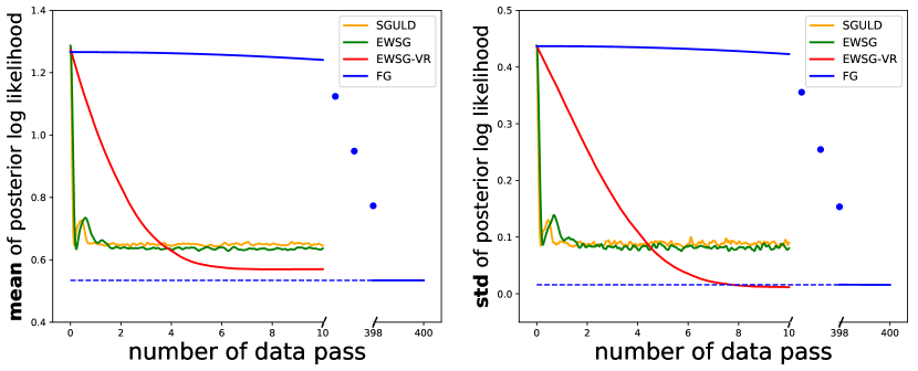
EWSG is derived based on matching transition kernels of MCMC and improves the accuracy of the entire distribution rather than just the variance. However, it does have a consequence of variance reduction and thus can be implicitly regarded as a VR method. When compared to the classic work on VR for SG-MCMC (Dubey et al., 2016), EWSG converges faster when the same amount of data pass is used, although its sampling accuracy is below that of VR for Gaussian targets (but well above vanilla SG; see Sec. 5.1). In this sense, EWSG and VR suit different application domains: EWSG can replace vanilla SG for tasks in which the priority is speed and then accuracy, as it keeps the speed but improves the accuracy; on the other hand, VR remains to be the heavy weapon for accuracy-demanding scenarios. Importantly, EWSG, as a generic way to improve SG-MCMC methods, can be combined with VR too (e.g., Sec. F); thus, they are not exclusive or competing with each other.

Importance Sampling (IS)

IS methods employ nonuniform weights to improve the convergence speed of stochastic gradient methods for optimization. Traditional IS methods use fixed weights that do not change along iterations, and the weight computation requires prior information of gradient terms, e.g., Lipschitz constant of the gradient (Needell et al., 2014; Schmidt et al., 2015; Csiba and Richtárik, 2018), which are usually unknown or difficult to estimate. Adaptive IS was also proposed in which the importance was re-evaluated at each iteration, whose computation usually required the entire data set per iteration and may also require information like the upper bound of gradient (Zhao and Zhang, 2015; Zhu, 2016).

For sampling, it is not easy to combine IS with SG (Fu and Zhang, 2017); the same paper is, to our knowledge, the closest to this goal and will be compared with in Sec. 5.3. EWSG can be viewed as a way to combine (adaptive) IS with SG for efficient sampling. It require no oracle about the gradient, nor any evaluation over the full data set. Instead, an inner-loop Metropolis chain maintains a random index that approximates a state-dependent non-uniform distribution (i.e. the weights/importance).

Other Mini-batch MCMC Methods

Besides SG-MCMC methods, there are also many non-gradient-based MCMC methods that use only a subset of data in each iteration so that the MCMC methods can scale to large data sets. For example, austerity MH (Korattikara et al., 2014) formulates Metropolis-Hastings step as a statistical hypothesis testing problem and proposes to use only a subset of data to make statistically significant accept/reject decision. Using a subsampled unbiased estimator of the likelihood in a pseudo-marginal framework to accelerate the Metropolis-Hastings algorithm is proposed in Bardenet et al. (2017). A notable exact MCMC method is FlyMC Maclaurin and Adams (2015), which introduces an auxiliary binary random variable for each datum and only the subset of data whose corresponding auxiliary binary indicator ”light” up, are used in iteration. Some more recent advances on exact MCMC methods include Zhang and De Sa (2019); Zhang et al. (2020). We also refer to Bardenet et al. (2017) for an excellent review on subsampling MCMC methods.

3 Underdamped Langevin: the continuous time backbone of a MCMC method

Underdamped Langevin Dynamics (ULD) is given by the SDE

{d𝜽=𝒓dtd𝒓=(V(𝜽)+γ𝒓)dt+σd𝑾cases𝑑𝜽absent𝒓𝑑𝑡𝑑𝒓absent𝑉𝜽𝛾𝒓𝑑𝑡𝜎𝑑𝑾\displaystyle\begin{cases}d\boldsymbol{\boldsymbol{\theta}}&=\boldsymbol{r}dt\\ d\boldsymbol{r}&=-(\nabla V(\boldsymbol{\boldsymbol{\theta}})+\gamma\boldsymbol{r})dt+\sigma d\boldsymbol{W}\end{cases} (1)

where 𝜽,𝒓d𝜽𝒓superscript𝑑\boldsymbol{\boldsymbol{\theta}},\boldsymbol{r}\in\mathbb{R}^{d} are state and momentum variables, V𝑉V is a potential energy function which in our context is, as originated from cost minimization or Bayesian inference over many data, the sum of many terms V(𝜽)=i=1nVi(𝜽)𝑉𝜽superscriptsubscript𝑖1𝑛subscript𝑉𝑖𝜽V(\boldsymbol{\boldsymbol{\theta}})=\sum_{i=1}^{n}V_{i}(\boldsymbol{\theta}), γ𝛾\gamma is a friction coefficient, σ𝜎\sigma is intrinsic noise amplitude, and 𝑾𝑾\boldsymbol{W} is a standard d𝑑d-dimensional Wiener process. Under mild assumptions on V𝑉V, Langevin dynamics admits a unique invariant distribution π(𝜽,𝒓)exp(1T(V(𝜽)+𝒓22))similar-to𝜋𝜽𝒓1𝑇𝑉𝜽superscriptnorm𝒓22\pi(\boldsymbol{\theta},\boldsymbol{r})\sim\exp\left(-\frac{1}{T}(V(\boldsymbol{\theta})+\frac{\|\boldsymbol{r}\|^{2}}{2})\right) and is in many cases geometric ergodic (Pavliotis, 2014). T𝑇T is the temperature of system determined via the fluctuation dissipation theorem σ2=2γTsuperscript𝜎22𝛾𝑇\sigma^{2}=2\gamma T (Kubo, 1966).

We consider ULD instead of the overdamped version mainly for two reasons: (i) one may think ULD is more complicated, and we’d like to show it is still easy to be paired with EWSG (EWSG can work for many MCMC methods; Appendix E has an overdamped version); (ii) it is believed that ULD has faster convergence than overdamped Langevin for instance in high-dimensions where (local) condition number is likely to be larger (e.g., Cheng et al. (2018b, a); Tao and Ohsawa (2020)). Like the overdamped version, numerical integrators for ULD with well captured statistical properties of the continuous process have been extensively investigated (e.g, Roberts et al. (1996); Bou-Rabee and Owhadi (2010)), and both the overdamped and underdamped integrators are friendly to derivations that will allow us to obtain explicit expressions of the non-uniform weights.

4 Method

4.1 Motivation: An Illustration of Non-optimality of Uniform Subsampling

Uniform subsampling of gradients have long been the dominant way of stochastic gradient approximations mainly because it is intuitive, unbiased and easy to implement.

However, uniform gradient subsampling can introduce large noise, and is sub-optimal even in the family of unbiased stochastic gradient estimator, as the following Theorem 1 will show. One intuition is, consider for example cases where data size n𝑛n is larger than dimension d𝑑d. In such cases, {Vi}i=1,2,,ndsubscriptsubscript𝑉𝑖𝑖12𝑛superscript𝑑\{\nabla V_{i}\}_{i=1,2,\cdots,n}\subset\mathbb{R}^{d} are linearly dependent and hence it is likely that there exist probability distributions {pi}i=1,2,,nsubscriptsubscript𝑝𝑖𝑖12𝑛\{p_{i}\}_{i=1,2,\cdots,n} other than the uniform one such that the gradient estimate is unbiased, however with smaller variance because linearly dependent terms need not to be all used. This is a motivation for us to develop non-uniform subsampling schemes (weights may be 𝜽𝜽\boldsymbol{\theta} dependent), although we will not require n>d𝑛𝑑n>d later.

Theorem 1

Suppose given 𝛉d𝛉superscript𝑑\boldsymbol{\theta}\in\mathbb{R}^{d}, the errors of SG approximation 𝐛i=nVi(𝛉)V(𝛉),1informulae-sequencesubscript𝐛𝑖𝑛subscript𝑉𝑖𝛉𝑉𝛉1𝑖𝑛\boldsymbol{b}_{i}=n\nabla V_{i}(\boldsymbol{\theta})-\nabla V(\boldsymbol{\theta}),1\leq i\leq n are i.i.d. absolutely continuous random vectors with possibly-𝛉𝛉\boldsymbol{\theta}-dependent density p(|𝛉)p(\cdot|\boldsymbol{\theta}) and n>d𝑛𝑑n>d. We call 𝐩n𝐩superscript𝑛\boldsymbol{p}\in\mathbb{R}^{n} a sparse vector if the number of non-zero entries in 𝐩𝐩\boldsymbol{p} is no greater than d+1𝑑1d+1, i.e. θ0d+1subscriptnorm𝜃0𝑑1\|\theta\|_{0}\leq d+1. Then with probability 111, the optimal probability distribution 𝐩superscript𝐩\boldsymbol{p}^{\star} that is unbiased and minimizes the trace of the covariance of nVI(𝛉)𝑛subscript𝑉𝐼𝛉n\nabla V_{I}(\boldsymbol{\theta}), i.e. 𝐩superscript𝐩\boldsymbol{p}^{\star} which solves the following, is a sparse vector.

min𝒑Tr(𝔼I𝒑[𝒃I𝒃IT])s.t. 𝔼I𝒑[𝒃I]=𝟎,subscript𝒑Trsubscript𝔼similar-to𝐼𝒑delimited-[]subscript𝒃𝐼superscriptsubscript𝒃𝐼𝑇s.t. subscript𝔼similar-to𝐼𝒑delimited-[]subscript𝒃𝐼0\displaystyle\min_{\boldsymbol{p}}\text{\rm Tr}(\mathbb{E}_{I\sim\boldsymbol{p}}[\boldsymbol{b}_{I}\boldsymbol{b}_{I}^{T}])\quad\text{s.t. }\mathbb{E}_{I\sim\boldsymbol{p}}[\boldsymbol{b}_{I}]=\boldsymbol{0}, (2)

Despite the sparsity of 𝒑superscript𝒑\boldsymbol{p}^{\star}, which seemingly suggests one only needs at most d+1𝑑1d+1 gradient terms per iteration when using SG methods, it is not practical because 𝒑superscript𝒑\boldsymbol{p}^{\star} requires solving the linear programming problem (2) in Theorem 1, for which an entire data pass is needed. Nevertheless, this result motivates us to seek alternatives to uniform SG. For example, the EWSG method we will develop will have reduced local variance with high probability, and at the same time remain efficiently implementable without having to use all data per parameter update; it can be biased though, but a global error analysis (Thm.3) will show that trading bias for variance can still be worthy.

4.2 Exponentially Weighted Stochastic Gradient

MCMC methods are characterized by their transition kernels. In traditional SG-MCMC methods, uniform SG is used, which is independent of the intrinsic randomness of MCMC methods (e.g. diffusion in ULD), as a result, the transition kernel of SG-MCMC is quite different from that with full gradient. Therefore, it is natural to ask — is it possible to couple the two originally independent randomness, so that the transition kernel of the SG-MCMC better matches that of the batch-gradient-MCMC, and the sampling accuracy is thus improved?

Here is one way to do so. Consider Euler-Maruyama (EM) discretization222EM is not the most accurate or robust discretization, see e.g., (Roberts et al., 1996; Bou-Rabee and Owhadi, 2010), but since it may still be the most used method, demonstrations here will be based on EM. The same idea of EWSG can easily apply to most other discretizations such as GLA (Bou-Rabee and Owhadi, 2010). of Eq. (1):

{𝜽k+1=𝜽k+𝒓kh𝒓k+1=𝒓k(V(𝜽k)+γ𝒓k)h+σh𝝃k+1casessubscript𝜽𝑘1absentsubscript𝜽𝑘subscript𝒓𝑘subscript𝒓𝑘1absentsubscript𝒓𝑘𝑉subscript𝜽𝑘𝛾subscript𝒓𝑘𝜎subscript𝝃𝑘1\begin{cases}\boldsymbol{\theta}_{k+1}&=\boldsymbol{\theta}_{k}+\boldsymbol{r}_{k}h\\ \boldsymbol{r}_{k+1}&=\boldsymbol{r}_{k}-(\nabla V(\boldsymbol{\theta}_{k})+\gamma\boldsymbol{r}_{k})h+\sigma\sqrt{h}\boldsymbol{\xi}_{k+1}\end{cases} (3)

where hh is step size and 𝝃k+1subscript𝝃𝑘1\boldsymbol{\xi}_{k+1}’s are i.i.d. d𝑑d-dimensional standard Gaussian random variables. Denote the transition kernel of EM discretization with full gradient by PEM(𝜽k+1,𝒓k+1|𝜽k,𝒓k)superscript𝑃𝐸𝑀subscript𝜽𝑘1conditionalsubscript𝒓𝑘1subscript𝜽𝑘subscript𝒓𝑘P^{EM}(\boldsymbol{\theta}_{k+1},\boldsymbol{r}_{k+1}|\boldsymbol{\theta}_{k},\boldsymbol{r}_{k}).

Then consider a SG version: replace V(𝜽k)𝑉subscript𝜽𝑘\nabla V(\boldsymbol{\theta}_{k}) by a weighted SG nVIk(𝜽k)𝑛subscript𝑉subscript𝐼𝑘subscript𝜽𝑘n\nabla V_{I_{k}}(\boldsymbol{\theta}_{k}), where Iksubscript𝐼𝑘I_{k} is the index chosen to approximate full gradient and has p.m.f. (Ik=i|𝜽k,𝒓k)=pisubscript𝐼𝑘conditional𝑖subscript𝜽𝑘subscript𝒓𝑘subscript𝑝𝑖\mathbb{P}(I_{k}=i|\boldsymbol{\theta}_{k},\boldsymbol{r}_{k})=p_{i}. Denote the new transition kernel by P~EM(𝜽k+1,𝒓k+1|𝜽k,𝒓k)superscript~𝑃𝐸𝑀subscript𝜽𝑘1conditionalsubscript𝒓𝑘1subscript𝜽𝑘subscript𝒓𝑘\tilde{P}^{EM}(\boldsymbol{\theta}_{k+1},\boldsymbol{r}_{k+1}|\boldsymbol{\theta}_{k},\boldsymbol{r}_{k}).

It is not hard to see that

PEM(𝜽k+1,𝒓k+1|𝜽k,𝒓k)superscript𝑃𝐸𝑀subscript𝜽𝑘1conditionalsubscript𝒓𝑘1subscript𝜽𝑘subscript𝒓𝑘\displaystyle P^{EM}(\boldsymbol{\theta}_{k+1},\boldsymbol{r}_{k+1}|\boldsymbol{\theta}_{k},\boldsymbol{r}_{k})
=\displaystyle= 1{𝜽k+𝒓kh}(𝜽k+1)1Zexp(𝒓k+1𝒓k+(V(𝜽k)+γ𝒓k)h22σ2h)subscript1subscript𝜽𝑘subscript𝒓𝑘subscript𝜽𝑘11𝑍superscriptnormsubscript𝒓𝑘1subscript𝒓𝑘𝑉subscript𝜽𝑘𝛾subscript𝒓𝑘22superscript𝜎2\displaystyle 1_{\{\boldsymbol{\theta}_{k}+\boldsymbol{r}_{k}h\}}(\boldsymbol{\theta}_{k+1})\,\frac{1}{Z}\exp\left(-\frac{\|\boldsymbol{r}_{k+1}-\boldsymbol{r}_{k}+(\nabla V(\boldsymbol{\theta}_{k})+\gamma\boldsymbol{r}_{k})h\|^{2}}{2\sigma^{2}h}\right)
=\displaystyle= 1{𝜽k+𝒓kh}(𝜽k+1)1Zexp(𝒙+i=1n𝒂i22)subscript1subscript𝜽𝑘subscript𝒓𝑘subscript𝜽𝑘11𝑍superscriptnorm𝒙superscriptsubscript𝑖1𝑛subscript𝒂𝑖22\displaystyle 1_{\{\boldsymbol{\theta}_{k}+\boldsymbol{r}_{k}h\}}(\boldsymbol{\theta}_{k+1})\,\frac{1}{Z}\exp\left(-\frac{\|\boldsymbol{x}+\sum_{i=1}^{n}\boldsymbol{a}_{i}\|^{2}}{2}\right)

and

P~EM(𝜽k+1,𝒓k+1|𝜽k,𝒓k)=1{𝜽k+𝒓kh}(𝜽k+1)1Z~j=1npiexp(𝒙+n𝒂i22),superscript~𝑃𝐸𝑀subscript𝜽𝑘1conditionalsubscript𝒓𝑘1subscript𝜽𝑘subscript𝒓𝑘subscript1subscript𝜽𝑘subscript𝒓𝑘subscript𝜽𝑘11~𝑍superscriptsubscript𝑗1𝑛subscript𝑝𝑖superscriptnorm𝒙𝑛subscript𝒂𝑖22\tilde{P}^{EM}(\boldsymbol{\theta}_{k+1},\boldsymbol{r}_{k+1}|\boldsymbol{\theta}_{k},\boldsymbol{r}_{k})=1_{\{\boldsymbol{\theta}_{k}+\boldsymbol{r}_{k}h\}}(\boldsymbol{\theta}_{k+1})\,\frac{1}{\tilde{Z}}\sum_{j=1}^{n}p_{i}\exp\left(-\frac{\|\boldsymbol{x}+n\boldsymbol{a}_{i}\|^{2}}{2}\right),

where Z𝑍Z and Z~~𝑍\tilde{Z} are normalization constants, 𝒙𝒓k+1𝒓k+hγ𝒓kσh𝒙subscript𝒓𝑘1subscript𝒓𝑘𝛾subscript𝒓𝑘𝜎\boldsymbol{x}\triangleq\frac{\boldsymbol{r}_{k+1}-\boldsymbol{r}_{k}+h\gamma\boldsymbol{r}_{k}}{\sigma\sqrt{h}} and 𝒂ihVi(𝜽k)σsubscript𝒂𝑖subscript𝑉𝑖subscript𝜽𝑘𝜎\boldsymbol{a}_{i}\triangleq\frac{\sqrt{h}\nabla V_{i}(\boldsymbol{\theta}_{k})}{\sigma}. From these two expressions, one can see that if we could choose

piexp(𝒙+i=1n𝒂i22+𝒙+n𝒂i22),proportional-tosubscript𝑝𝑖superscriptnorm𝒙superscriptsubscript𝑖1𝑛subscript𝒂𝑖22superscriptnorm𝒙𝑛subscript𝒂𝑖22p_{i}\propto\exp\left(-\frac{\|\boldsymbol{x}+\sum_{i=1}^{n}\boldsymbol{a}_{i}\|^{2}}{2}+\frac{\|\boldsymbol{x}+n\boldsymbol{a}_{i}\|^{2}}{2}\right), (4)

we would have PEM(𝜽k+1,𝒓k+1|𝜽k,𝒓k)=P~EM(𝜽k+1,𝒓k+1|𝜽k,𝒓k)superscript𝑃𝐸𝑀subscript𝜽𝑘1conditionalsubscript𝒓𝑘1subscript𝜽𝑘subscript𝒓𝑘superscript~𝑃𝐸𝑀subscript𝜽𝑘1conditionalsubscript𝒓𝑘1subscript𝜽𝑘subscript𝒓𝑘P^{EM}(\boldsymbol{\theta}_{k+1},\boldsymbol{r}_{k+1}|\boldsymbol{\theta}_{k},\boldsymbol{r}_{k})=\tilde{P}^{EM}(\boldsymbol{\theta}_{k+1},\boldsymbol{r}_{k+1}|\boldsymbol{\theta}_{k},\boldsymbol{r}_{k}) and be able to recover the transition kernel of full gradient with that of stochastic gradient. However, Eq.(4) is only formal and infeasible, because 𝒙𝒙\boldsymbol{x} is dependent on the future state variable 𝒓k+1subscript𝒓𝑘1\boldsymbol{r}_{k+1} which we do not know. Therefore, to obtain a practically implementable algorithm, we will fix 𝒙𝒙\boldsymbol{x} as a hyper-parameter and hope that the approximation is good enough so that we still have PEM(𝜽k+1,𝒓k+1|𝜽k,𝒓k)P~EM(𝜽k+1,𝒓k+1|𝜽k,𝒓k)superscript𝑃𝐸𝑀subscript𝜽𝑘1conditionalsubscript𝒓𝑘1subscript𝜽𝑘subscript𝒓𝑘superscript~𝑃𝐸𝑀subscript𝜽𝑘1conditionalsubscript𝒓𝑘1subscript𝜽𝑘subscript𝒓𝑘P^{EM}(\boldsymbol{\theta}_{k+1},\boldsymbol{r}_{k+1}|\boldsymbol{\theta}_{k},\boldsymbol{r}_{k})\approx\tilde{P}^{EM}(\boldsymbol{\theta}_{k+1},\boldsymbol{r}_{k+1}|\boldsymbol{\theta}_{k},\boldsymbol{r}_{k}).

We refer to the choice of pisubscript𝑝𝑖p_{i} in eq.4 Exponentially Weighted Stochastic Gradient (EWSG). Unlike Thm.1, EWSG does not require n>d𝑛𝑑n>d to work. Note the idea of designing non-uniform weights of SG-MCMC to match the transition kernel of full gradient can be suitably applied to a wide class of gradient-based MCMC methods; for example, Sec. E shows how EWSG can be applied to Langevin Monte Carlo (overdamped Langevin), and Sec. F shows how it can be combined with VR. Therefore, EWSG complements a wide range of SG-MCMC methods.

Since the weight choice of EWSG is motivated by approximating the transition kernel of a full-gradient MCMC method, we anticipate EWSG to be statistically more accurate than a uniformly-subsampled stochastic gradient estimator. As a special but commonly interested accuracy measure, the smaller variance of EWSG is shown with high probability333‘With high probability’ but not almost surely because Theorem 2 in fact suits a class of weights, which includes but is not limited to EWSG.:

Theorem 2

Assume {Vi(𝛉)}i=1,2,,nsubscriptsubscript𝑉𝑖𝛉𝑖12𝑛\{\nabla V_{i}(\boldsymbol{\theta})\}_{i=1,2,\cdots,n} are i.i.d random vectors and |Vi(𝛉)|Rsubscript𝑉𝑖𝛉𝑅|\nabla V_{i}(\boldsymbol{\theta})|\leq R for some constant R𝑅R almost surely. Denote the uniform distribution over [n]delimited-[]𝑛[n] by 𝐩Usuperscript𝐩𝑈\boldsymbol{p}^{U}, the exponentially weighted distribution by 𝐩Esuperscript𝐩𝐸\boldsymbol{p}^{E}, and let Δ=Tr[covI𝐩E[nVI(𝛉)|𝛉]covI𝐩U[nVI(𝛉)|𝛉]]ΔTrsubscriptcovsimilar-to𝐼superscript𝐩𝐸delimited-[]conditional𝑛subscript𝑉𝐼𝛉𝛉subscriptcovsimilar-to𝐼superscript𝐩𝑈delimited-[]conditional𝑛subscript𝑉𝐼𝛉𝛉\Delta=\operatorname{Tr}[\text{\rm cov}_{I\sim\boldsymbol{p}^{E}}[n\nabla V_{I}(\boldsymbol{\theta})|\boldsymbol{\theta}]-\text{\rm cov}_{I\sim\boldsymbol{p}^{U}}[n\nabla V_{I}(\boldsymbol{\theta})|\boldsymbol{\theta}]]. If 𝐱=𝒪(h)𝐱𝒪\boldsymbol{x}=\mathcal{O}(\sqrt{h}), we have 𝔼[Δ]<0𝔼delimited-[]Δ0\mathbb{E}[\Delta]<0, and C>0𝐶0\exists C>0 independent of n𝑛n or hh such that ϵ>0for-allitalic-ϵ0\forall\epsilon>0,

(|Δ𝔼[Δ]|ϵ)2exp(ϵ2nCh2).Δ𝔼delimited-[]Δitalic-ϵ2superscriptitalic-ϵ2𝑛𝐶superscript2\mathbb{P}(|\Delta-\mathbb{E}[\Delta]|\geq\epsilon)\leq 2\exp\left(-\frac{\epsilon^{2}}{nCh^{2}}\right).

It is not surprising that less non-intrinsic local variance correlates with better global statistical accuracy, which will be made explicit and rigorous in the next subsection.

4.3 Non-asymptotic Error Bound

We now establish a non-asymptotic global sampling error bound (in mean square distance between arbitrary test observables) of SG underdamped Langevin algorithms (the bound applies to both EWSG and other methods e.g., SGHMC). The full proof is deferred to the Appendix C, but the main tool we will be using is the Poisson equation machinery (Mattingly et al., 2010; Vollmer et al., 2016; Chen et al., 2015). A brief overview is the following:

Let 𝑿=(𝜽𝒓)𝑿matrix𝜽𝒓\boldsymbol{X}=\left(\begin{matrix}\boldsymbol{\theta}\\ \boldsymbol{r}\end{matrix}\right). The generator \mathcal{L} of diffusion process (1) is

(f(𝑿t))=𝑓subscript𝑿𝑡absent\displaystyle\mathcal{L}(f(\boldsymbol{X}_{t}))= limh0𝔼[f(𝑿t+h)]𝔼[f(𝑿t)]hsubscript0𝔼delimited-[]𝑓subscript𝑿𝑡𝔼delimited-[]𝑓subscript𝑿𝑡\displaystyle\lim_{h\to 0}\frac{\mathbb{E}[f(\boldsymbol{X}_{t+h})]-\mathbb{E}[f(\boldsymbol{X}_{t})]}{h}
=\displaystyle= 𝒓T𝜽f(γ𝒓+V(𝜽))T𝒓f+γΔ𝒓f.superscript𝒓𝑇subscript𝜽𝑓superscript𝛾𝒓𝑉𝜽𝑇subscript𝒓𝑓𝛾subscriptΔ𝒓𝑓\displaystyle\boldsymbol{r}^{T}\nabla_{\boldsymbol{\theta}}f-(\gamma\boldsymbol{r}+\nabla V(\boldsymbol{\theta}))^{T}\nabla_{\boldsymbol{r}}f+\gamma\Delta_{\boldsymbol{r}}f.

Given a test function ϕ(𝒙)italic-ϕ𝒙\phi(\boldsymbol{x}), its posterior average is ϕ¯=ϕ(𝒙)π(𝒙)𝑑𝒙¯italic-ϕitalic-ϕ𝒙𝜋𝒙differential-d𝒙\bar{\phi}=\int\phi(\boldsymbol{x})\pi(\boldsymbol{x})d\boldsymbol{x}, approximated by its time average of samples ϕ^K=1Kk=1Kϕ(𝑿kE)subscript^italic-ϕ𝐾1𝐾superscriptsubscript𝑘1𝐾italic-ϕsubscriptsuperscript𝑿𝐸𝑘\widehat{\phi}_{K}=\frac{1}{K}\sum_{k=1}^{K}\phi(\boldsymbol{X}^{E}_{k}), where 𝑿kEsuperscriptsubscript𝑿𝑘𝐸\boldsymbol{X}_{k}^{E} is the sample path given by EM integrator. Then the Poisson equation ψ=ϕϕ¯𝜓italic-ϕ¯italic-ϕ\mathcal{L}\psi=\phi-\bar{\phi} can be a useful tool for the weak convergence analysis of SG-MCMC. The solution ψ𝜓\psi characterizes the difference between ϕitalic-ϕ\phi and its posterior average ϕ¯¯italic-ϕ\bar{\phi}.

Our main theoretical result is the following:

Theorem 3

Assume 𝔼[Vi(𝛉kE)l]<M1,𝔼[𝐫kEl]<M2,l=1,2,,12,i=1,2,,nformulae-sequence𝔼delimited-[]superscriptnormsubscript𝑉𝑖subscriptsuperscript𝛉𝐸𝑘𝑙subscript𝑀1formulae-sequence𝔼delimited-[]superscriptnormsubscriptsuperscript𝐫𝐸𝑘𝑙subscript𝑀2formulae-sequencefor-all𝑙1212for-all𝑖12𝑛\mathbb{E}[\|\nabla V_{i}(\boldsymbol{\theta}^{E}_{k})\|^{l}]<M_{1},\mathbb{E}[\|\boldsymbol{r}^{E}_{k}\|^{l}]<M_{2},\forall l=1,2,\cdots,12,\forall i=1,2,\cdots,n and k0for-all𝑘0\forall k\geq 0. Assume the solution to the Poisson equation, ψ𝜓\psi, exists, and its derivatives up to 3rd-order are uniformly bounded Dlψ<M3,l=0,1,2,3formulae-sequencesubscriptnormsuperscript𝐷𝑙𝜓subscript𝑀3𝑙0123\|D^{l}\psi\|_{\infty}<M_{3},l=0,1,2,3. Then there exist constants C1,C2,C3>0subscript𝐶1subscript𝐶2subscript𝐶30C_{1},C_{2},C_{3}>0 depending on M1,M2,M3subscript𝑀1subscript𝑀2subscript𝑀3M_{1},M_{2},M_{3}, such that

𝔼(ϕ^Kϕ¯)2C11T+C2hTk=0K1𝔼[Tr[cov(nVIk|k)]]K+C3h2𝔼superscriptsubscript^italic-ϕ𝐾¯italic-ϕ2subscript𝐶11𝑇subscript𝐶2𝑇superscriptsubscript𝑘0𝐾1𝔼delimited-[]Trcovconditional𝑛subscript𝑉subscript𝐼𝑘subscript𝑘𝐾subscript𝐶3superscript2\mathbb{E}\big{(}\widehat{\phi}_{K}-\bar{\phi}\big{)}^{2}\leq C_{1}\frac{1}{T}+C_{2}\frac{h}{T}\frac{\sum_{k=0}^{K-1}\mathbb{E}[\operatorname{Tr}[\mbox{\rm cov}(n\nabla V_{I_{k}}|\mathcal{F}_{k})]]}{K}+C_{3}h^{2} (5)

where T=Kh𝑇𝐾T=Kh is the corresponding time in the underlying continuous dynamics, Iksubscript𝐼𝑘I_{k} is the index of the datum used to estimate the gradient at k𝑘k-th iteration, and cov(nVIk|k)covconditional𝑛subscript𝑉subscript𝐼𝑘subscript𝑘\mbox{cov}(n\nabla V_{I_{k}}|\mathcal{F}_{k}) is the covariance of stochastic gradient at k𝑘k-th iteration conditioned on the current sigma algebra ksubscript𝑘\mathcal{F}_{k} in the filtration.

Remark: (interpreting the three terms in the bound) Unlike a typical VR method which aims at finding unbiased gradient estimator with reduced variance, EWSG aims at bringing the entire density closer to that of a batch-gradient MCMC. As a consequence, its practical implementation may correspond to SG that has reduced variance but a small bias too. Eq.(5) quantifies this bias-variance trade-off. How the extrinsic local variance and bias contribute to the global error is respectively reflected in the 2nd and 3rd terms, although the 3rd term also contains a contribution from the numerical discretization error. With or without bias, the 3rd term remains 𝒪(h2)𝒪superscript2\mathcal{O}(h^{2}) because of this discretization error. However, for moderate T𝑇T, the 2nd term is generally larger than the 3rd due to its lower order in hh, which means reducing local variance can improve sampling accuracy even if at the cost of introducing a small bias. Since EWSG has a smaller local variance than uniform SG (Thm.2, as a special case of improved overall statistical accuracy), its global performance is also favorable. The 1st term is for the convergence of the continuous process (eq.1 in this case).

Remark: (innovation and relation with the literature) Thm.3, to the best of our knowledge, is the first that incorporates the effects of both local bias and local variance of a SG approximation (previous SOTA bounds are only for unbiased SG). It still works when restricting to unbiased SG, and in this case our bound reduces to SOTA Vollmer et al. (2016); Chen et al. (2015). Some more facts include: Mattingly et al. (2010), being the seminal work from which we adapt our proof, only discussed the batch gradient case, whereas our theory has additional (non-uniform) SG. Vollmer et al. (2016); Chen et al. (2015) studied the effect of SG, but the SG considered there did not use state-dependent weights, which would destroy several martingales used in their proofs. Unlike in Mattingly et al. (2010) but like in Vollmer et al. (2016); Chen et al. (2015), our state space is not the compact torus but dsuperscript𝑑\mathbb{R}^{d}. Also, the time average ϕ^Ksubscript^italic-ϕ𝐾\widehat{\phi}_{K}, to which our results apply, is a commonly used estimator, particularly when using a long time trajectory of Markov chain for sampling. However, if one is interested in an alternative of using an ensemble for sampling, techniques in Cheng et al. (2018b); Dalalyan and Karagulyan (2017) might be useful to further bound difference between the law of 𝑿ksubscript𝑿𝑘\boldsymbol{X}_{k} and the target distribution.

4.4 Practical Implementation

In EWSG, the probability of each gradient term is pi=Z^1exp{𝒙+j=1n𝒂j22+𝒙+n𝒂i22}subscript𝑝𝑖superscript^𝑍1superscriptnorm𝒙superscriptsubscript𝑗1𝑛subscript𝒂𝑗22superscriptnorm𝒙𝑛subscript𝒂𝑖22p_{i}=\widehat{Z}^{-1}\exp\left\{-\frac{\|\boldsymbol{x}+\sum_{j=1}^{n}\boldsymbol{a}_{j}\|^{2}}{2}+\frac{\|\boldsymbol{x}+n\boldsymbol{a}_{i}\|^{2}}{2}\right\}. Although the term 𝒙+j=1n𝒂j2/2superscriptnorm𝒙superscriptsubscript𝑗1𝑛subscript𝒂𝑗22\|\boldsymbol{x}+\sum_{j=1}^{n}\boldsymbol{a}_{j}\|^{2}/2 depends on the full data set, it is shared by all pisubscript𝑝𝑖p_{i}’s and can be absorbed into the normalization constant Z^1superscript^𝑍1\hat{Z}^{-1} (we still included it explicitly due to the needs in proofs); unique to each pisubscript𝑝𝑖p_{i} is only the term 𝒙+n𝒂i2/2superscriptnorm𝒙𝑛subscript𝒂𝑖22\|\boldsymbol{x}+n\boldsymbol{a}_{i}\|^{2}/2. This motivates us to run a Metropolis-Hastings chain over the possible indices i{1,2,n}𝑖12𝑛i\in\{1,2\,\cdots,n\}: at each inner-loop step, a proposal of index j𝑗j is uniformly drawn, and then accepted with probability P(ij)=𝑃𝑖𝑗absentP(i\to j)=

min{1,exp(𝒙+n𝒂j22𝒙+n𝒂i22)};1superscriptnorm𝒙𝑛subscript𝒂𝑗22superscriptnorm𝒙𝑛subscript𝒂𝑖22\min\left\{1,\exp\left(\frac{\|\boldsymbol{x}+n\boldsymbol{a}_{j}\|^{2}}{2}-\frac{\|\boldsymbol{x}+n\boldsymbol{a}_{i}\|^{2}}{2}\right)\right\}; (6)

if accepted, the current index i𝑖i is replaced by j𝑗j. When the chain converges, the index will follow the distribution given by pisubscript𝑝𝑖p_{i}. The advantage is, we avoid passing through the entire data sets to compute each pisubscript𝑝𝑖p_{i}, but the index will still approximately sample from the non-uniform distribution.

In practice, we often perform only M=1𝑀1M=1 step of the Metropolis index chain per integration step, especially if hh is not too large. The rationale is, when hh is small, the outer iteration evolves slower than the index chain, and as θ𝜃\theta does not change much in, say, N𝑁N outer steps, effectively N×M𝑁𝑀N\times M inner steps take place on almost the same index chain, which makes the index r.v. equilibrate better. Regarding the larger hh case (where the efficacy of local variance reduction via non-uniform subsampling is more pronounced; see e.g., Thm. 3), M=1𝑀1M=1 may no longer be optimal, but improved sampling with large hh and M=1𝑀1M=1 is still clearly observed in various experiments (Sec. 5).

Another hyper-parameter is 𝒙𝒙\boldsymbol{x} (see earlier discussion in Sec.4.2). Our heuristic recommendation is 𝒙=hγ𝒓kσ𝒙𝛾subscript𝒓𝑘𝜎\boldsymbol{x}=\frac{\sqrt{h}\gamma\boldsymbol{r}_{k}}{\sigma}. The rationale is, as long as rk+1rksubscript𝑟𝑘1subscript𝑟𝑘r_{k+1}-r_{k}’s density is maximized at 0 (which will be the case at least for large k𝑘k as rksubscript𝑟𝑘r_{k} will converge to a Gaussian), this choice of 𝒙𝒙\boldsymbol{x} is a maximum likelihood estimator. This approximation appeared to be a good one in all our experiments with medium hh and M=1𝑀1M=1.

Sec. 5.1 further investigates hyperparameter selection empirically and shows that approximations due to M𝑀M and 𝒙𝒙\boldsymbol{x} is not detrimental to our non-asymptotic theory in Sec. 4.3.

Practical EWSG is summarized in Algorithm 1. For simplicity of notation, we restrict the description to mini batch size b=1𝑏1b=1, but an extension to b>1𝑏1b>1 is straightforward. See Sec. D in appendix. Practical EWSG has reduced variance but does not completely eliminate the extrinsic noise created by SG due to its approximations. A small bias was also created by these approximations, but its effect is dominated by the variance effect (see Sec. 4.3). In practice, if needed, one can combine EWSG with other VR technique to further improve accuracy. Appendix F describes how EWSG can be combined with SVRG.

Algorithm 1 EWSG
  Input: {the number of data terms n𝑛n, gradient functions Vi(),i=1,2,,nformulae-sequencesubscript𝑉𝑖𝑖12𝑛V_{i}(\cdot),i=1,2,\cdots,n, step size hh, the number of data passes K𝐾K, index chain length M𝑀M, friction and noise coefficients γ𝛾\gamma and σ𝜎\sigma}
  Initialize 𝜽0,𝒓0subscript𝜽0subscript𝒓0\boldsymbol{\theta}_{0},\boldsymbol{r}_{0} (arbitrarily, or use an informed guess)
  for k=0,1,,KnM+1𝑘01𝐾𝑛𝑀1k=0,1,\cdots,\lceil\frac{Kn}{M+1}\rceil do
     i𝑖absenti\leftarrow uniformly sampled from 1,,n1𝑛{1,\cdots,n},   compute and store nVi(𝜽k)𝑛subscript𝑉𝑖subscript𝜽𝑘n\nabla V_{i}(\boldsymbol{\theta}_{k})
     Ii𝐼𝑖I\leftarrow i
     for m=1,2,,M𝑚12𝑀m=1,2,\cdots,M do
        j𝑗absentj\leftarrow uniformly sampled from 1,,n1𝑛{1,\cdots,n},   compute and store nVj(𝜽k)𝑛subscript𝑉𝑗subscript𝜽𝑘n\nabla V_{j}(\boldsymbol{\theta}_{k})
        Ij𝐼𝑗I\leftarrow j with probability in Equation 6
     end for
     Evaluate V~(𝜽k)=nVI(𝜽k)~𝑉subscript𝜽𝑘𝑛subscript𝑉𝐼subscript𝜽𝑘\tilde{V}(\boldsymbol{\theta}_{k})=nV_{I}(\boldsymbol{\theta}_{k})
     Update (𝜽k+1,𝒓k+1)(𝜽k,𝒓k)subscript𝜽𝑘1subscript𝒓𝑘1subscript𝜽𝑘subscript𝒓𝑘(\boldsymbol{\theta}_{k+1},\boldsymbol{r}_{k+1})\leftarrow(\boldsymbol{\theta}_{k},\boldsymbol{r}_{k}) via one step of Euler-Maruyama integration using V~(𝜽k)~𝑉subscript𝜽𝑘\tilde{V}(\boldsymbol{\theta}_{k})
  end for

5 Experiments

In this section, the proposed EWSG algorithm will be compared with SGHMC (Chen et al., 2014), SGLD (Welling and Teh, 2011), as well as several more recent popular approaches, including FlyMC (Maclaurin and Adams, 2015), pSGLD (Li et al., 2016), CP-SGHMC (Fu and Zhang, 2017) (a method closest to the goal of applying IS idea to SG-based sampling) and SVRG-LD (Dubey et al., 2016) (overdamped Langevin improved by VR). Sec. 5.1 is a detailed empirical study of EWSG on simple models, with comparison and implication of two important hyper-parameters M𝑀M and 𝒙𝒙\boldsymbol{x}, and verification of the non-asymptotic theory (Theorem 3). Sec. 5.2 demonstrates EWSG for Bayesian logistic regression on a large-scale data set. Sec. 5.3 is a Bayesian Neural Network (BNN) example. It serves only as a high-dimensional, multi-modal test case, and we do not intend to compare Bayesian and non-Bayesian neural nets. As FlyMC requires a tight lower bound of likelihood, known for only a few cases, it will only be compared against in Sec. 5.2 where such a bound is obtainable. CP-SGHMC requires heavy tuning on the number of clusters which differs across data sets/algorithms, so it will only be included in the BNN example, for which the authors empirically found a good hyper parameter for MNIST (Fu and Zhang, 2017). SVRG-LD is only compared to in Sec. 5.1, because SG-MCMC methods can converge within only one data pass in Sec. 5.2, rendering control-variate based VR technique inapplicable, and it was suggested that VR leads to poor results for deep models (e.g., Sec. 5.3) (Defazio and Bottou, 2019).

For fair comparison, all algorithms use constant step sizes and are allowed fixed computation budget, i.e., for L𝐿L data passes, all algorithms can only call gradient function nL𝑛𝐿nL times. All experiments are conducted on a machine with a 2.20GHz Intel(R) Xeon(R) E5-2630 v4 CPU and an Nvidia GeForce GTX 1080 GPU. If not otherwise mentioned, σ=2γ𝜎2𝛾\sigma=\sqrt{2\gamma} so only γ𝛾\gamma needs specification, the length of the index chain is set M=1𝑀1M=1 for EWSG and the default values of two hyper-parameters required in pSGLD are set λ=105𝜆superscript105\lambda=10^{-5} and α=0.99𝛼0.99\alpha=0.99, as suggested in Li et al. (2016).

5.1 Gaussian Examples

Consider sampling from a simple 2D Gaussian whose potential function is

V(𝜽)=i=1nVi(𝜽)=i=1n12𝜽𝒄i2.𝑉𝜽superscriptsubscript𝑖1𝑛subscript𝑉𝑖𝜽superscriptsubscript𝑖1𝑛12superscriptnorm𝜽subscript𝒄𝑖2V(\boldsymbol{\theta})=\sum_{i=1}^{n}V_{i}(\boldsymbol{\theta})=\sum_{i=1}^{n}\frac{1}{2}\|\boldsymbol{\theta}-\boldsymbol{c}_{i}\|^{2}.

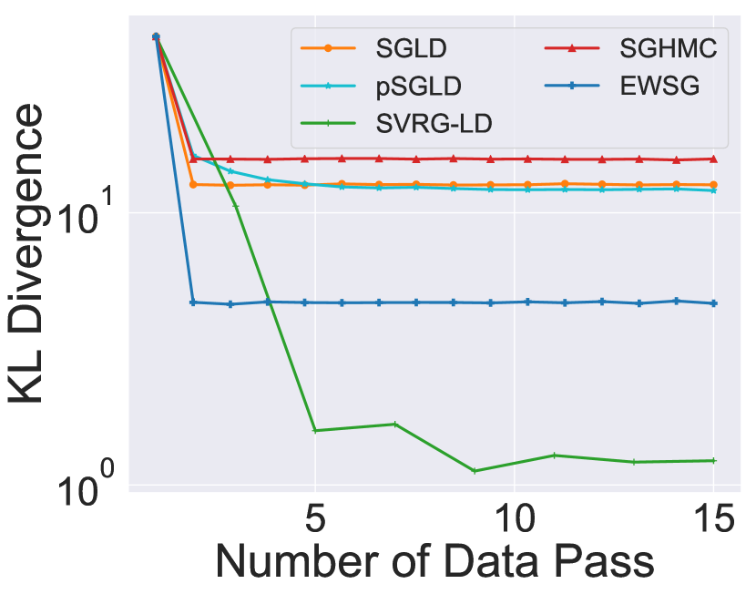
We set n=50𝑛50n=50 and randomize 𝒄isubscript𝒄𝑖\boldsymbol{c}_{i} from a two-dimensional standard normal 𝒩(𝟎,I2)𝒩0subscript𝐼2\mathcal{N}(\boldsymbol{0},I_{2}). Due to the simplicity of V(𝜽)𝑉𝜽V(\boldsymbol{\theta}), we can write the target density analytically and will use KL divergence KL(pq)=p(𝜽)logp(𝜽)q(𝜽)d𝜽KLconditional𝑝𝑞𝑝𝜽𝑝𝜽𝑞𝜽𝑑𝜽\mathrm{KL}(p\|q)=\int p(\boldsymbol{\theta})\log\frac{p(\boldsymbol{\theta})}{q(\boldsymbol{\theta})}d\boldsymbol{\theta} to measure the difference between the target distribution and generated samples.
Refer to caption
(a) Sample quality in KL
Refer to caption
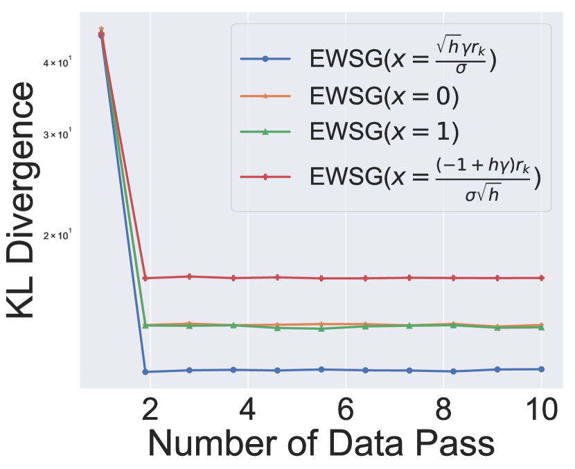
(b) Performance for various 𝒙𝒙\boldsymbol{x}
Refer to caption
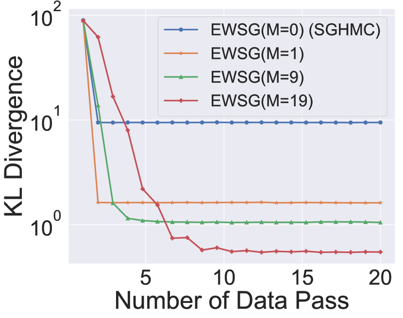
(c) Performance for various M𝑀M
Refer to caption
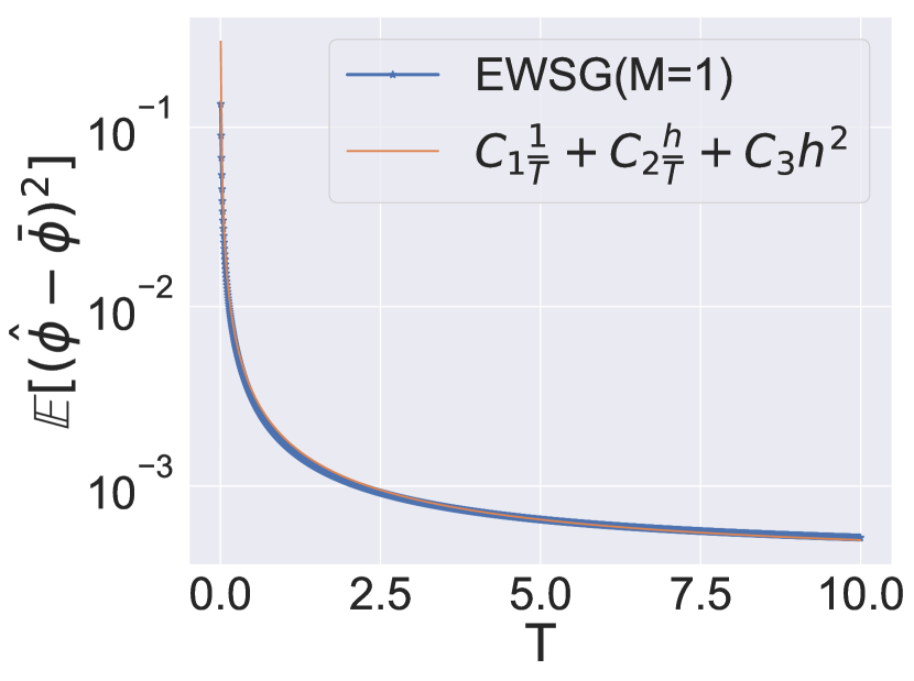
(d) MSE against time T𝑇T (1st and 2nd terms in Eq. (5))
Refer to caption
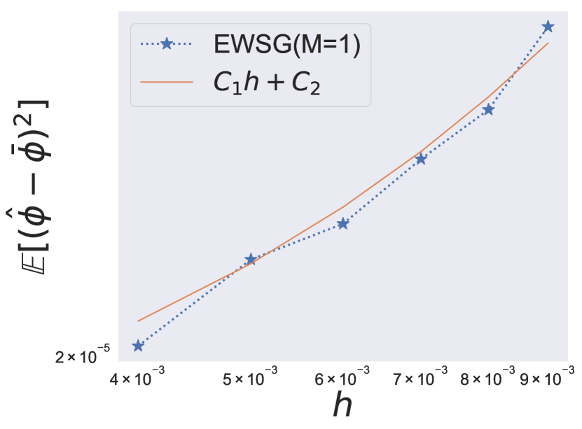
(e) MSE against step size hh with fixed finite T𝑇T (2nd term in Eq. (5))
Refer to caption
(f) MSE against step size hh with T𝑇T\approx\infty (3rd term in Eq. (5))
Figure 1: Sampling from Gaussian target

For each algorithm, we generate 10,000 independent realizations for empirical estimation. All algorithms are run for 30 data passes with minibatch size of 1. Step size is tuned from 5×{101,102,103,104}5superscript101superscript102superscript103superscript1045\times\{10^{-1},10^{-2},10^{-3},10^{-4}\} and 5×1035superscript1035\times 10^{-3} is chosen for SGLD and pSGLD, 5×1025superscript1025\times 10^{-2} for SGHMC and EWSG and 5×1045superscript1045\times 10^{-4} for SVRG-LD. SGHMC and EWSG use γ=10𝛾10\gamma=10. Results are shown in Fig. 1(a) and EWSG outperforms SGHMC, SGLD and pSGLD in terms of accuracy. Note SVRG-LD has the best accuracy444For Gaussians, mean and variance completely determine the distribution, so appropriately reduced variance leads to great accuracy for the entire distribution. but the slowest convergence, and that is why EWSG is a useful alternative to VR: its light-weight suits situations with limited computational resources better.

Figure 1(b) shows the performance of several possible choices of the hyper-parameter 𝒙𝒙\boldsymbol{x}, including the recommended option 𝒙=hγ𝒓k/σ𝒙𝛾subscript𝒓𝑘𝜎\boldsymbol{x}=\sqrt{h}\gamma\boldsymbol{r}_{k}/\sigma, and 𝒙=𝟎𝒙0\boldsymbol{x}=\boldsymbol{0}, 𝒙=𝟏𝒙1\boldsymbol{x}=\boldsymbol{1}, 𝒙=(1+hγ)𝒓k/σh𝒙1𝛾subscript𝒓𝑘𝜎\boldsymbol{x}=(-1+h\gamma)\boldsymbol{r}_{k}/\sigma\sqrt{h} (which corresponds to 𝒓k+1=𝟎subscript𝒓𝑘10\boldsymbol{r}_{k+1}=\boldsymbol{0}). Step size h=7×1027superscript102h=7\times 10^{-2} is used for this experiment. The recommended option performs better than the others.

Another important hyper-parameter in EWSG is M𝑀M. As the length of index chain M𝑀M increases, the subsampling distribution approaches that given by Eq.4. Considering that larger M𝑀M means more gradient evaluations per step555in each iteration of the outer MCMC loop, EWSG consumes M+1𝑀1M+1 data points, and hence in a fair comparison with fixed computation budget (e.g. E𝐸E total gradient calls), EWSG runs EM+1𝐸𝑀1\frac{E}{M+1} iterations which is decreasing in M𝑀M., there could be some M𝑀M value that achieves the best balance between speed and accuracy. Fig.1(c) shows a fair comparison of four values of M=0,1,9,19𝑀01919M=0,1,9,19, and the recommended M=1𝑀1M=1 case converges as fast as SGHMC (when M=0𝑀0M=0, EWSG does not run the Metropolis-Hastings index chain and hence degenerates to SGHMC) but improves its accuracy. It is also clear that as M𝑀M increases, sampling accuracy gets improved.

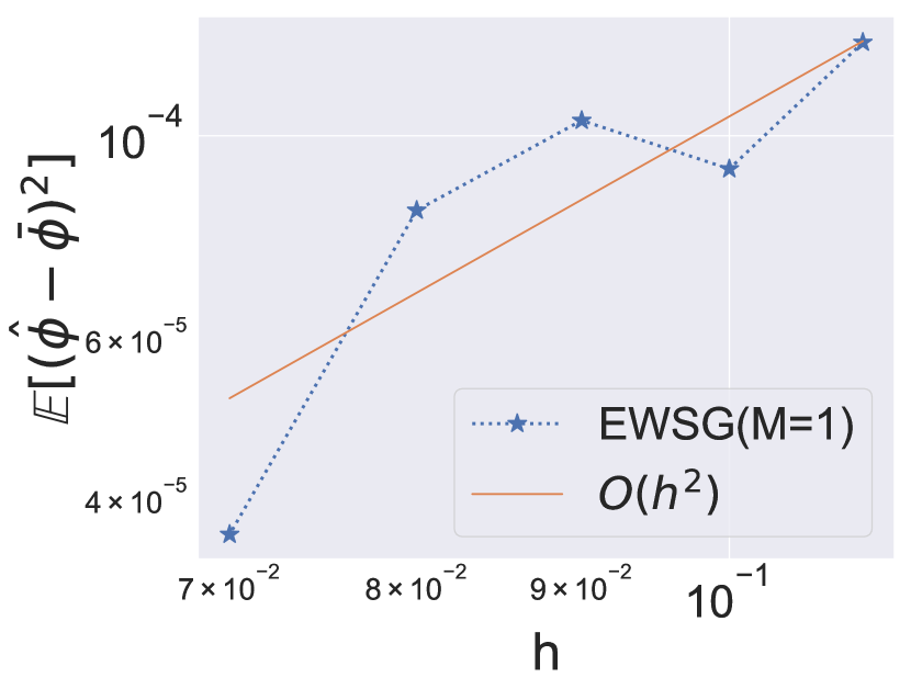
As approximations are used in Algorithm 1, it is natural to ask if results of Thm. 3 still hold. We empirically investigate this question (using M=1𝑀1M=1 and variance as the test function ϕitalic-ϕ\phi). Eq.5 in Thm.3 is a nonasymptotic error bound consisting of three parts, namely an 𝒪(1T)𝒪1𝑇\mathcal{O}(\frac{1}{T}) term corresponding to the convergence at the continuous limit, an 𝒪(h/T)𝒪𝑇\mathcal{O}(h/T) term coming from the SG variance, and an 𝒪(h2)𝒪superscript2\mathcal{O}(h^{2}) term due to bias and numerical error. Fig.1(d) plots the mean squared error (MSE) against time T=Kh𝑇𝐾T=Kh to confirm the 1st term. Fig.1(e) plots the MSE against hh with fixed T𝑇T in the small hh regime (so that the 3rd term is negligible when compared to the 2nd) to confirm that the 2nd term scales like 𝒪(h)𝒪\mathcal{O}(h). For the 3rd term in Eq. (5), we run sufficiently many iterations to ensure all chains are well-mixed, and Fig.1(f) confirms the final MSE to scale like 𝒪(h2)𝒪superscript2\mathcal{O}(h^{2}) even for large hh (as the 2nd term vanishes due to T𝑇T\to\infty). In this sense, despite the approximations introduced by the practical implementation, the performance of Algorithm 1 is still approximated by Thm. 3, even when M=1𝑀1M=1. Thm. 3 can thus guide the choices of hh and T𝑇T in practice.

  Method SGLD pSGLD SGHMC EWSG FlyMC
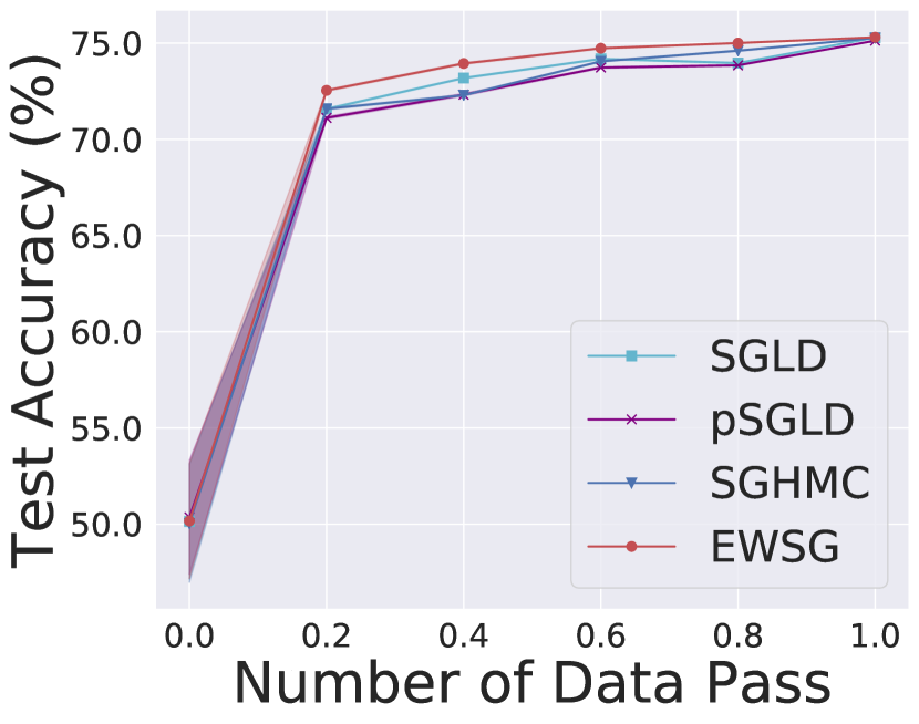
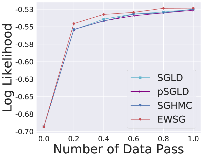
Accuracy(%) 75.283 ±plus-or-minus\pm 0.016 75.126 ±plus-or-minus\pm 0.020 75.268 ±plus-or-minus\pm 0.017 75.306 ±plus-or-minus\pm 0.016 75.199 ±plus-or-minus\pm 0.080
Log Likelihood -0.525 ±plus-or-minus\pm 0.000 -0.526 ±plus-or-minus\pm 0.000 -0.525 ±plus-or-minus\pm 0.000 -0.523 ±plus-or-minus\pm 0.000 -0.523 ±plus-or-minus\pm 0.000
Wall Time (s) 3.085 ±plus-or-minus\pm 0.283 4.312 ±plus-or-minus\pm 0.359 3.145 ±plus-or-minus\pm 0.307 3.755 ±plus-or-minus\pm 0.387 291.295 ±plus-or-minus\pm 56.368
 
Table 1: Accuracy, log likelihood and wall time of various algorithms on test data after one data pass (mean ±plus-or-minus\pm std).

5.2 Bayesian Logistic Regression (BLR)

Consider Bayesian logistic regression for the binary classification problem. The probabilistic model for predicting a label yksubscript𝑦𝑘y_{k} given a feature vector xksubscript𝑥𝑘x_{k} is p(yk=1|𝒙k,𝜽)=1/(1+exp(𝜽T𝒙k))𝑝subscript𝑦𝑘conditional1subscript𝒙𝑘𝜽11superscript𝜽𝑇subscript𝒙𝑘p(y_{k}=1|\boldsymbol{x}_{k},\boldsymbol{\theta})=1/(1+\exp(-\boldsymbol{\theta}^{T}\boldsymbol{x}_{k})). We set a Gaussian prior with zero mean and covariance Σ=10IdΣ10subscript𝐼𝑑\Sigma=10I_{d} for 𝜽𝜽\boldsymbol{\theta}, and hence the potential function of the posterior distribution of 𝜽𝜽\boldsymbol{\theta} is

V(𝜽)=5𝜽2i=1nyilogp(yi=1|𝒙i,𝜽)+(1yi)log(1p(yi=1|𝒙i,𝜽)).𝑉𝜽5superscriptnorm𝜽2superscriptsubscript𝑖1𝑛subscript𝑦𝑖𝑝subscript𝑦𝑖conditional1subscript𝒙𝑖𝜽1subscript𝑦𝑖1𝑝subscript𝑦𝑖conditional1subscript𝒙𝑖𝜽V(\boldsymbol{\theta})=5\|\boldsymbol{\theta}\|^{2}-\sum_{i=1}^{n}y_{i}\log p(y_{i}=1|\boldsymbol{x}_{i},\boldsymbol{\theta})+(1-y_{i})\log\left(1-p(y_{i}=1|\boldsymbol{x}_{i},\boldsymbol{\theta})\right).

We conduct our experiments on Covertype data set666https://archive.ics.uci.edu/ml/datasets/covertype, which contains n=581,012𝑛581012n=581,012 data points and 54 features (which is the dimension of 𝜽𝜽\boldsymbol{\theta}). Given the large size of this data set, SG is needed to scale up MCMC methods. We use 80% of data for training and the rest 20% for testing.

The FlyMC algorithm777https://github.com/HIPS/firefly-monte-carlo/tree/master/flymc uses a lower bound derived in Maclaurin and Adams (2015) for likelihood function. For underdamped Langevin based algorithms, we set friction coefficient γ=50𝛾50\gamma=50. After tuning, we set the step size as {1,3,0.02,5,5}×103130.0255superscript103\{1,3,0.02,5,5\}\times 10^{-3} for SGULD, EWSG, SGLD, pSGLD and FlyMC. All algorithms are run for one data pass, with minibatch size of 50 (for FlyMC, it means 50 data are sampled in each iteration to switch state). 100 independent samples are drawn from each algorithm to estimate statistics. To further smooth out noise, all experiments are repeated 1000 times with different seeds.

Results are in Fig. 2(a) and 2(b) and Table 1. EWSG outperforms others, except for log likelihood being comparable to FlyMC, which is an exact MCMC method. The wall time consumed by EWSG is only slightly more than that of SGLD and SGHMC, but less than pSGLD and orders-of-magnitude less than FlyMC.
Refer to caption
(a) Test Accuracy
Refer to caption
(b) Test Log Likelihood
Figure 2: BLR learning curve
Refer to caption
(c) MLP architecture
Refer to caption
(d) CNN architecture
Figure 3: BNN learning curve. Shade: one standard deviation.

5.3 Bayesian Neural Network (BNN)

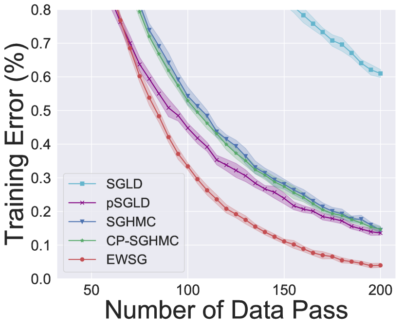
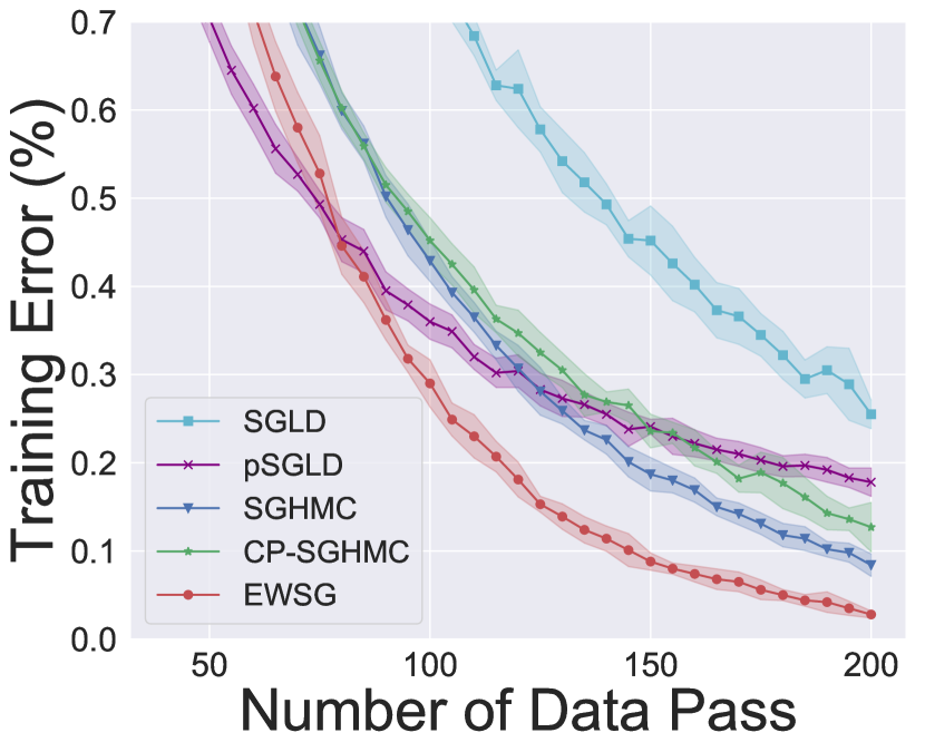
Bayesian neural network is a compelling model for deep learning (Wilson, 2020). Here two popular architectures of BNN are experimented – multilayer perceptron (MLP) and convolutional neural nets (CNN). In MLP, a hidden layer with 100 neurons followed by a softmax layer is used. In CNN, we use standard network configuration with 2 convolutional layers followed by 2 fully connected layers (Jarrett et al., 2009). Both convolutional layers use 5×5555\times 5 convolution kernel with 32 and 64 channels, 2×2222\times 2 max pooling layers follow immediately after convolutional layer. The last two fully-connected layers each has 200 neurons. We set the standard normal as prior for all weights and bias.

We test algorithms on the MNIST data set, consisting of 60,000 training data and 10,000 test data, each datum is a 28×28282828\times 28 gray-scale image with one of the ten possible labels (digits 09similar-to090\sim 9). For ULD based algorithms , we set friction coefficient γ=0.1𝛾0.1\gamma=0.1 in MLP and γ=1.0𝛾1.0\gamma=1.0 in CNN. In MLP, the step sizes are set h={4,2,2}×103422superscript103h=\{4,2,2\}\times 10^{-3} for EWSG, SGHMC and CP-SGHMC, and h={0.001,1}×1040.0011superscript104h=\{0.001,1\}\times 10^{-4} for SGLD and pSGLD, via grid search. For CP-SGHMC , (clustering-based preprocessing is conducted (Fu and Zhang, 2017) before SGHMC) we use K-means with 10 clusters to preprocess the data set. In CNN, the step sizes are set h={4,2,2}×103422superscript103h=\{4,2,2\}\times 10^{-3} for EWSG, SGHMC and CP-SGHMC, and h={0.02,8}×1060.028superscript106h=\{0.02,8\}\times 10^{-6} for SGLD and pSGLD, via grid search. All algorithms use minibatch size of 100 and are run for 200 epoches. For each algorithm, we generate 100 independent samples to make posterior prediction. To smooth out noise and obtain more significant results, we repeat experiments 10 times with different seeds.

The learning curve of training error is shown in Fig. 2(c) and 2(d). EWSG consistently improves over its uniform counterpart (i.e., SGHMC) and CP-SGHMC (an approximate IS SG-MCMC). Moreover, EWSG also outperforms two standard benchmarks SGLD and pSGLD. The improvement over baseline on MNIST data set is comparable to some of the early works (Chen et al., 2014; Li et al., 2016).

Note: in the MLP setup, the model has d>78,400𝑑78400d>78,400 parameters whereas there are n=60,000𝑛60000n=60,000 data points, which shows EWSG does not require n>d𝑛𝑑n>d to work and can still outperform its uniform counterpart in the overparametrized regime (Thm.1 demonstrates the underparametrized case only because the sparsity result is easy to understand, but EWSG doesn’t only work for underparameterized models).

Acknowledgment

We thank Yian Ma and Xuefeng Gao for insightful discussions. MT is grateful for the partial support by NSF DMS-1847802 and ECCS-1936776. This work was mainly conducted when HZ was a professor at Georgia Institute of Technology.

References

  • Ahn et al. (2012) Sungjin Ahn, Anoop Korattikara, and Max Welling. Bayesian posterior sampling via stochastic gradient fisher scoring. In 29th International Conference on Machine Learning, ICML 2012, pages 1591–1598, 2012.
  • Bach (2013) Francis Bach. Stochastic gradient methods for machine learning. Technical report, INRIA - Ecole Normale Superieur, 2013. URL http://lear.inrialpes.fr/people/harchaoui/projects/gargantua/slides/bach_gargantua_nov2013.pdf.
  • Baker et al. (2019) Jack Baker, Paul Fearnhead, Emily B Fox, and Christopher Nemeth. Control variates for stochastic gradient mcmc. Statistics and Computing, 29(3):599–615, 2019.
  • Bardenet et al. (2017) Rémi Bardenet, Arnaud Doucet, and Christopher C Holmes. On markov chain monte carlo methods for tall data. Journal of Machine Learning Research, 18(47), 2017.
  • Borkar and Mitter (1999) Vivek S Borkar and Sanjoy K Mitter. A strong approximation theorem for stochastic recursive algorithms. Journal of optimization theory and applications, 100(3):499–513, 1999.
  • Bou-Rabee and Owhadi (2010) Nawaf Bou-Rabee and Houman Owhadi. Long-run accuracy of variational integrators in the stochastic context. SIAM Journal on Numerical Analysis, 48(1):278–297, 2010.
  • Bou-Rabee and Sanz-Serna (2018) Nawaf Bou-Rabee and Jesús María Sanz-Serna. Geometric integrators and the Hamiltonian Monte Carlo method. Acta Numerica, 27:113–206, 2018.
  • Bou-Rabee et al. (2018) Nawaf Bou-Rabee, Andreas Eberle, and Raphael Zimmer. Coupling and convergence for Hamiltonian Monte Carlo. arXiv preprint arXiv:1805.00452, 2018.
  • Brooks et al. (2011) Steve Brooks, Andrew Gelman, Galin Jones, and Xiao-Li Meng. Handbook of markov chain monte carlo. CRC press, 2011.
  • Chatterji et al. (2018) Niladri S Chatterji, Nicolas Flammarion, Yi-An Ma, Peter L Bartlett, and Michael I Jordan. On the theory of variance reduction for stochastic gradient monte carlo. ICML, 2018.
  • Chen et al. (2015) Changyou Chen, Nan Ding, and Lawrence Carin. On the convergence of stochastic gradient mcmc algorithms with high-order integrators. In Advances in Neural Information Processing Systems, pages 2278–2286, 2015.
  • Chen et al. (2014) Tianqi Chen, Emily B Fox, and Carlos Guestrin. Stochastic Gradient Hamiltonian Monte Carlo. International Conference on Machine Learning, pages 1683–1691, 2014.
  • Cheng et al. (2018a) Xiang Cheng, Niladri S Chatterji, Yasin Abbasi-Yadkori, Peter L Bartlett, and Michael I Jordan. Sharp convergence rates for langevin dynamics in the nonconvex setting. arXiv preprint arXiv:1805.01648, 2018a.
  • Cheng et al. (2018b) Xiang Cheng, Niladri S Chatterji, Peter L Bartlett, and Michael I Jordan. Underdamped langevin mcmc: A non-asymptotic analysis. Proceedings of the 31st Conference On Learning Theory, PMLR, 2018b.
  • Csiba and Richtárik (2018) Dominik Csiba and Peter Richtárik. Importance sampling for minibatches. The Journal of Machine Learning Research, 19(1):962–982, 2018.
  • Dalalyan and Karagulyan (2017) Arnak S Dalalyan and Avetik G Karagulyan. User-friendly guarantees for the langevin monte carlo with inaccurate gradient. arXiv preprint arXiv:1710.00095, 2017.
  • Defazio and Bottou (2019) Aaron Defazio and Léon Bottou. On the ineffectiveness of variance reduced optimization for deep learning. In Advances in Neural Information Processing Systems, pages 1755–1765, 2019.
  • Defazio et al. (2014) Aaron Defazio, Francis Bach, and Simon Lacoste-Julien. Saga: A fast incremental gradient method with support for non-strongly convex composite objectives. In Advances in neural information processing systems, pages 1646–1654, 2014.
  • Dubey et al. (2016) Kumar Avinava Dubey, Sashank J Reddi, Sinead A Williamson, Barnabas Poczos, Alexander J Smola, and Eric P Xing. Variance reduction in stochastic gradient langevin dynamics. In Advances in neural information processing systems, pages 1154–1162, 2016.
  • Fu and Zhang (2017) Tianfan Fu and Zhihua Zhang. Cpsg-mcmc: Clustering-based preprocessing method for stochastic gradient mcmc. In Artificial Intelligence and Statistics, pages 841–850, 2017.
  • Jarrett et al. (2009) Kevin Jarrett, Koray Kavukcuoglu, Marc’Aurelio Ranzato, and Yann LeCun. What is the best multi-stage architecture for object recognition? In 2009 IEEE 12th international conference on computer vision, pages 2146–2153. IEEE, 2009.
  • Johnson and Zhang (2013) Rie Johnson and Tong Zhang. Accelerating stochastic gradient descent using predictive variance reduction. In Advances in neural information processing systems, pages 315–323, 2013.
  • Korattikara et al. (2014) Anoop Korattikara, Yutian Chen, and Max Welling. Austerity in mcmc land: Cutting the metropolis-hastings budget. In International Conference on Machine Learning, pages 181–189. PMLR, 2014.
  • Kubo (1966) Rep Kubo. The fluctuation-dissipation theorem. Reports on progress in physics, 29(1):255, 1966.
  • Li et al. (2016) Chunyuan Li, Changyou Chen, David Carlson, and Lawrence Carin. Preconditioned stochastic gradient langevin dynamics for deep neural networks. In Thirtieth AAAI Conference on Artificial Intelligence, 2016.
  • Li et al. (2017) Qianxiao Li, Cheng Tai, and E Weinan. Stochastic modified equations and adaptive stochastic gradient algorithms. In International Conference on Machine Learning, pages 2101–2110, 2017.
  • Li et al. (2021) Ruilin Li, Hongyuan Zha, and Molei Tao. Mean-square analysis with an application to optimal dimension dependence of Langevin Monte Carlo. preprint arXiv:2109.03839, 2021.
  • Lichman et al. (2013) Moshe Lichman et al. UCI machine learning repository, 2013.
  • Ma et al. (2015) Yi-An Ma, Tianqi Chen, and Emily Fox. A complete recipe for stochastic gradient mcmc. In Advances in Neural Information Processing Systems, pages 2917–2925, 2015.
  • Maclaurin and Adams (2015) Dougal Maclaurin and Ryan Prescott Adams. Firefly monte carlo: Exact mcmc with subsets of data. In Twenty-Fourth International Joint Conference on Artificial Intelligence, 2015.
  • Mandt et al. (2017) Stephan Mandt, Matthew D Hoffman, and David M Blei. Stochastic gradient descent as approximate bayesian inference. The Journal of Machine Learning Research, 18(1):4873–4907, 2017.
  • Mattingly et al. (2010) Jonathan C Mattingly, Andrew M Stuart, and Michael V Tretyakov. Convergence of numerical time-averaging and stationary measures via poisson equations. SIAM Journal on Numerical Analysis, 48(2):552–577, 2010.
  • Needell et al. (2014) Deanna Needell, Rachel Ward, and Nati Srebro. Stochastic gradient descent, weighted sampling, and the randomized kaczmarz algorithm. In Advances in Neural Information Processing Systems, pages 1017–1025, 2014.
  • Patterson and Teh (2013) Sam Patterson and Yee Whye Teh. Stochastic gradient Riemannian Langevin dynamics on the probability simplex. Advances in Neural Information Processing Systems, pages 3102–3110, 2013.
  • Pavliotis (2014) Grigorios A Pavliotis. Stochastic processes and applications: diffusion processes, the Fokker-Planck and Langevin equations, volume 60. Springer, 2014.
  • Roberts et al. (1996) Gareth O Roberts, Richard L Tweedie, et al. Exponential convergence of langevin distributions and their discrete approximations. Bernoulli, 2(4):341–363, 1996.
  • Schmidt et al. (2015) Mark Schmidt, Reza Babanezhad, Mohamed Ahmed, Aaron Defazio, Ann Clifton, and Anoop Sarkar. Non-uniform stochastic average gradient method for training conditional random fields. In artificial intelligence and statistics, pages 819–828, 2015.
  • Schmidt et al. (2017) Mark Schmidt, Nicolas Le Roux, and Francis Bach. Minimizing finite sums with the stochastic average gradient. Mathematical Programming, 162(1-2):83–112, 2017.
  • Tao and Ohsawa (2020) Molei Tao and Tomoki Ohsawa. Variational optimization on lie groups, with examples of leading (generalized) eigenvalue problems. AISTATS, 2020.
  • Teh et al. (2016) Yee Whye Teh, Alexandre H Thiery, and Sebastian J Vollmer. Consistency and fluctuations for stochastic gradient langevin dynamics. The Journal of Machine Learning Research, 17(1):193–225, 2016.
  • Vollmer et al. (2016) Sebastian J Vollmer, Konstantinos C Zygalakis, and Yee Whye Teh. Exploration of the (non-) asymptotic bias and variance of stochastic gradient langevin dynamics. The Journal of Machine Learning Research, 17(1):5504–5548, 2016.
  • Welling and Teh (2011) Max Welling and Yee Whye Teh. Bayesian learning via stochastic gradient langevin dynamics. International Conference on Machine Learning, pages 681–688, 2011.
  • Wilson (2020) Andrew Gordon Wilson. The case for bayesian deep learning. arXiv preprint arXiv:2001.10995, 2020.
  • Zhang and De Sa (2019) Ruqi Zhang and Christopher De Sa. Poisson-minibatching for gibbs sampling with convergence rate guarantees. NeurIPS, 2019.
  • Zhang et al. (2020) Ruqi Zhang, A Feder Cooper, and Christopher De Sa. Asymptotically optimal exact minibatch metropolis-hastings. NeurIPS, 2020.
  • Zhao and Zhang (2015) Peilin Zhao and Tong Zhang. Stochastic optimization with importance sampling for regularized loss minimization. In International Conference on Machine Learning, pages 1–9, 2015.
  • Zhu (2016) Rong Zhu. Gradient-based sampling: An adaptive importance sampling for least-squares. In Advances in Neural Information Processing Systems, pages 406–414, 2016.

Appendix A Proof of Theorem 1

Proof: Denote the set of all n𝑛n-dimensional probability vectors by ΣnsuperscriptΣ𝑛\Sigma^{n}, the set of sparse probability vectors by 𝒮𝒮\mathcal{S}, and the set of non-sparse (dense) probability vectors by 𝒟=Σn𝒮𝒟superscriptΣ𝑛𝒮\mathcal{D}=\Sigma^{n}\setminus\mathcal{S}. Denote B=[𝒃1,,𝒃n]𝐵subscript𝒃1subscript𝒃𝑛B=[\boldsymbol{b}_{1},\cdots,\boldsymbol{b}_{n}], then the optimization problem can be written as

mini=1npi𝒃i2superscriptsubscript𝑖1𝑛subscript𝑝𝑖superscriptnormsubscript𝒃𝑖2\displaystyle\min\sum_{i=1}^{n}p_{i}\|\boldsymbol{b}_{i}\|^{2}
s.t.{B𝒑=𝟎𝒑T𝟏n=1pi0,i=1,2,,ns.t.cases𝐵𝒑0otherwisesuperscript𝒑𝑇subscript1𝑛1otherwiseformulae-sequencesubscript𝑝𝑖0𝑖12𝑛otherwise\displaystyle\text{s.t.}\begin{cases}\displaystyle B\boldsymbol{p}=\boldsymbol{0}\\ \boldsymbol{p}^{T}\boldsymbol{1}_{n}=1\\ p_{i}\geq 0,i=1,2,\cdots,n\end{cases}

Note that the feasible region is always non-empty (take 𝒑𝒑\boldsymbol{p} to be a uniform distribution) and is also closed and bounded, hence this linear programming is always solvable. Denote the set of all minimizers by \mathcal{M}. Note that \mathcal{M} depends on 𝒃1,,𝒃nsubscript𝒃1subscript𝒃𝑛\boldsymbol{b}_{1},\cdots,\boldsymbol{b}_{n} and is in this sense random.

The Lagrange function is

L(𝒑,𝝀,μ,𝝎)=𝒑T𝒔𝝀TB𝒑μ(𝒑T𝟏n)𝝎T𝒑𝐿𝒑𝝀𝜇𝝎superscript𝒑𝑇𝒔superscript𝝀𝑇𝐵𝒑𝜇superscript𝒑𝑇subscript1𝑛superscript𝝎𝑇𝒑L(\boldsymbol{p},\boldsymbol{\lambda},\mu,\boldsymbol{\omega})=\boldsymbol{p}^{T}\boldsymbol{s}-\boldsymbol{\lambda}^{T}B\boldsymbol{p}-\mu(\boldsymbol{p}^{T}\boldsymbol{1}_{n})-\boldsymbol{\omega}^{T}\boldsymbol{p}

where 𝒔=[𝒃12,𝒃22,,𝒃n2]T𝒔superscriptsuperscriptnormsubscript𝒃12superscriptnormsubscript𝒃22superscriptnormsubscript𝒃𝑛2𝑇\boldsymbol{s}=[\|\boldsymbol{b}_{1}\|^{2},\|\boldsymbol{b}_{2}\|^{2},\cdots,\|\boldsymbol{b}_{n}\|^{2}]^{T} and 𝝀,μ,𝝎𝝀𝜇𝝎\boldsymbol{\lambda},\mu,\boldsymbol{\omega} are dual variables. The optimality condition reads as

L𝒑=𝒔BT𝝀μ𝟏n𝝎=𝟎𝐿𝒑𝒔superscript𝐵𝑇𝝀𝜇subscript1𝑛𝝎0\frac{\partial L}{\partial\boldsymbol{p}}=\boldsymbol{s}-B^{T}\boldsymbol{\lambda}-\mu\boldsymbol{1}_{n}-\boldsymbol{\omega}=\boldsymbol{0}

Dual feasibilty and complementary slackness require

ωi0,i=1,2,,nformulae-sequencesubscript𝜔𝑖0𝑖12𝑛\displaystyle\omega_{i}\leq 0,i=1,2,\cdots,n
𝝎T𝒑=0superscript𝝎𝑇𝒑0\displaystyle\boldsymbol{\omega}^{T}\boldsymbol{p}=0

Consider the probability of the event {a dense probability vector can solve the above minimization problem}, i.e., (𝒟)𝒟\mathbb{P}(\mathcal{M}\cap\mathcal{D}\neq\emptyset). It is upper bounded by

(𝒟)(𝒑𝒟 and 𝒑 solves KKT condition)𝒟𝒑𝒟 and 𝒑 solves KKT condition\mathbb{P}(\mathcal{M}\cap\mathcal{D}\neq\emptyset)\leq\mathbb{P}(\boldsymbol{p}\in\mathcal{D}\mbox{ and }\boldsymbol{p}\mbox{ solves KKT condition})

Since 𝒑𝒟𝒑𝒟\boldsymbol{p}\in\mathcal{D}, complementary slackness implies that at least d+2𝑑2d+2 entries in 𝝎𝝎\boldsymbol{\omega} are zero. Denote the indices of these entries by 𝒥𝒥\mathcal{J}. For every j𝒥𝑗𝒥j\in\mathcal{J}, by optimality condition, we have sj𝝀T𝒃jμ=0subscript𝑠𝑗superscript𝝀𝑇subscript𝒃𝑗𝜇0s_{j}-\boldsymbol{\lambda}^{T}\boldsymbol{b}_{j}-\mu=0, i.e.,

𝒃j2𝝀T𝒃jμ=0superscriptnormsubscript𝒃𝑗2superscript𝝀𝑇subscript𝒃𝑗𝜇0\|\boldsymbol{b}_{j}\|^{2}-\boldsymbol{\lambda}^{T}\boldsymbol{b}_{j}-\mu=0

Take the first d+1𝑑1d+1 indices in 𝒥𝒥\mathcal{J}, and note a geometric fact that d+1𝑑1d+1 points in a d𝑑d-dimensional space must be on the surface of a hypersphere of at most d1𝑑1d-1 dimension, which we denote by 𝒮=Sq1+𝒙𝒮superscript𝑆𝑞1𝒙\mathcal{S}=S^{q-1}+\boldsymbol{x} for some vector 𝒙𝒙\boldsymbol{x} and integer qd𝑞𝑑q\leq d. Because bisubscript𝑏𝑖b_{i}’s distribution is absolutely continuous, we have

(𝒑𝒟 and 𝒑 solves KKT condition)𝒑𝒟 and 𝒑 solves KKT condition\displaystyle\mathbb{P}(\boldsymbol{p}\in\mathcal{D}\mbox{ and }\boldsymbol{p}\mbox{ solves KKT condition})
\displaystyle\leq (𝒑𝒟 and 𝒃jS,j𝒥)\displaystyle\mathbb{P}(\boldsymbol{p}\in\mathcal{D}\mbox{ and }\boldsymbol{b}_{j}\in S,\forall j\in\mathcal{J})
\displaystyle\leq (𝒃jS,j𝒥)formulae-sequencesubscript𝒃𝑗𝑆for-all𝑗𝒥\displaystyle\mathbb{P}(\boldsymbol{b}_{j}\in S,\forall j\in\mathcal{J})
=\displaystyle= (𝒃jkS,k=d+2,,|𝒥|)formulae-sequencesubscript𝒃subscript𝑗𝑘𝑆𝑘𝑑2𝒥\displaystyle\mathbb{P}(\boldsymbol{b}_{j_{k}}\in S,k=d+2,\cdots,|\mathcal{J}|)
=\displaystyle= k=d+2|𝒥|(𝒃jkS)(independence)superscriptsubscriptproduct𝑘𝑑2𝒥subscript𝒃subscript𝑗𝑘𝑆(independence)\displaystyle\prod_{k=d+2}^{|\mathcal{J}|}\mathbb{P}(\boldsymbol{b}_{j_{k}}\in S)\qquad\mbox{(independence)}
=\displaystyle= 0(absolute continuous)0(absolute continuous)\displaystyle 0\qquad\mbox{(absolute continuous)}

Hence (𝒟)=0𝒟0\mathbb{P}(\mathcal{M}\cap\mathcal{D}\neq\emptyset)=0 and

11\displaystyle 1 =()absent\displaystyle=\mathbb{P}(\mathcal{M}\neq\emptyset)
=((𝒮)(𝒟))absent𝒮𝒟\displaystyle=\mathbb{P}((\mathcal{M}\cap\mathcal{S})\cup(\mathcal{M}\cap\mathcal{D})\neq\emptyset)
(𝒮)+(𝒟)absent𝒮𝒟\displaystyle\leq\mathbb{P}(\mathcal{M}\cap\mathcal{S}\neq\emptyset)+\mathbb{P}(\mathcal{M}\cap\mathcal{D}\neq\emptyset)
=(𝒮)absent𝒮\displaystyle=\mathbb{P}(\mathcal{M}\cap\mathcal{S}\neq\emptyset)

Therefore we have

(𝒮)=1𝒮1\mathbb{P}(\mathcal{M}\cap\mathcal{S}\neq\emptyset)=1


Appendix B Proof of Theorem 2

Proof: Let 𝒃i=nVisubscript𝒃𝑖𝑛subscript𝑉𝑖\boldsymbol{b}_{i}=n\nabla V_{i} and assume 𝒃i2Rsubscriptnormsubscript𝒃𝑖2𝑅\|\boldsymbol{b}_{i}\|_{2}\leq R for some constant R𝑅R. Denote B=[𝒃1,𝒃2,,𝒃n]𝐵subscript𝒃1subscript𝒃2subscript𝒃𝑛B=[\boldsymbol{b}_{1},\boldsymbol{b}_{2},\cdots,\boldsymbol{b}_{n}]. For any probability distribution 𝒑𝒑\boldsymbol{p} over {1,,n}1𝑛\{1,\cdots,n\}, we have

covI𝒑[𝒃I|𝒃1,,𝒃n]subscriptcovsimilar-to𝐼𝒑delimited-[]conditionalsubscript𝒃𝐼subscript𝒃1subscript𝒃𝑛\displaystyle\text{cov}_{I\sim\boldsymbol{p}}[\boldsymbol{b}_{I}|\boldsymbol{b}_{1},\cdots,\boldsymbol{b}_{n}]
=\displaystyle= i=1npi𝒃i𝒃iT(i=1npi𝒃i)(i=1npi𝒃i)Tsuperscriptsubscript𝑖1𝑛subscript𝑝𝑖subscript𝒃𝑖superscriptsubscript𝒃𝑖𝑇superscriptsubscript𝑖1𝑛subscript𝑝𝑖subscript𝒃𝑖superscriptsuperscriptsubscript𝑖1𝑛subscript𝑝𝑖subscript𝒃𝑖𝑇\displaystyle\sum_{i=1}^{n}p_{i}\boldsymbol{b}_{i}\boldsymbol{b}_{i}^{T}-\left(\sum_{i=1}^{n}p_{i}\boldsymbol{b}_{i}\right)\left(\sum_{i=1}^{n}p_{i}\boldsymbol{b}_{i}\right)^{T}
=\displaystyle= i=1npi𝒃i𝒃iTi=1npi(i=1npi𝒃i)(i=1npi𝒃i)Tsuperscriptsubscript𝑖1𝑛subscript𝑝𝑖subscript𝒃𝑖superscriptsubscript𝒃𝑖𝑇superscriptsubscript𝑖1𝑛subscript𝑝𝑖superscriptsubscript𝑖1𝑛subscript𝑝𝑖subscript𝒃𝑖superscriptsuperscriptsubscript𝑖1𝑛subscript𝑝𝑖subscript𝒃𝑖𝑇\displaystyle\sum_{i=1}^{n}p_{i}\boldsymbol{b}_{i}\boldsymbol{b}_{i}^{T}\sum_{i=1}^{n}p_{i}-\left(\sum_{i=1}^{n}p_{i}\boldsymbol{b}_{i}\right)\left(\sum_{i=1}^{n}p_{i}\boldsymbol{b}_{i}\right)^{T}
=\displaystyle= i<j(𝒃i𝒃j)(𝒃i𝒃j)Tpipjsubscript𝑖𝑗subscript𝒃𝑖subscript𝒃𝑗superscriptsubscript𝒃𝑖subscript𝒃𝑗𝑇subscript𝑝𝑖subscript𝑝𝑗\displaystyle\sum_{i<j}(\boldsymbol{b}_{i}-\boldsymbol{b}_{j})(\boldsymbol{b}_{i}-\boldsymbol{b}_{j})^{T}p_{i}p_{j}

Therefore we let

f(B):=assign𝑓𝐵absent\displaystyle f(B):= Tr[i<j(𝒃i𝒃j)(𝒃i𝒃j)Tpipji<j(𝒃i𝒃j)(𝒃i𝒃j)T1n2]Trsubscript𝑖𝑗subscript𝒃𝑖subscript𝒃𝑗superscriptsubscript𝒃𝑖subscript𝒃𝑗𝑇subscript𝑝𝑖subscript𝑝𝑗subscript𝑖𝑗subscript𝒃𝑖subscript𝒃𝑗superscriptsubscript𝒃𝑖subscript𝒃𝑗𝑇1superscript𝑛2\displaystyle\operatorname{Tr}\left[\sum_{i<j}(\boldsymbol{b}_{i}-\boldsymbol{b}_{j})(\boldsymbol{b}_{i}-\boldsymbol{b}_{j})^{T}p_{i}p_{j}-\sum_{i<j}(\boldsymbol{b}_{i}-\boldsymbol{b}_{j})(\boldsymbol{b}_{i}-\boldsymbol{b}_{j})^{T}\frac{1}{n^{2}}\right]
=\displaystyle= i<j𝒃i𝒃j2pipji<j𝒃i𝒃j21n2(Tr[AB]=Tr[BA])subscript𝑖𝑗superscriptnormsubscript𝒃𝑖subscript𝒃𝑗2subscript𝑝𝑖subscript𝑝𝑗subscript𝑖𝑗superscriptnormsubscript𝒃𝑖subscript𝒃𝑗21superscript𝑛2Tr𝐴𝐵Tr𝐵𝐴\displaystyle\sum_{i<j}\|\boldsymbol{b}_{i}-\boldsymbol{b}_{j}\|^{2}p_{i}p_{j}-\sum_{i<j}\|\boldsymbol{b}_{i}-\boldsymbol{b}_{j}\|^{2}\frac{1}{n^{2}}\qquad(\operatorname{Tr}[AB]=\operatorname{Tr}[BA])

and use it to compare the trace of covariance matrix of uniform- and nonuniform- subsamplings.

First of all,

𝔼[f(B)]𝔼delimited-[]𝑓𝐵\displaystyle\mathbb{E}[f(B)]
=\displaystyle= 𝔼[𝒃i𝒃j2]i<j(pipj1n2)𝔼delimited-[]superscriptnormsubscript𝒃𝑖subscript𝒃𝑗2subscript𝑖𝑗subscript𝑝𝑖subscript𝑝𝑗1superscript𝑛2\displaystyle\mathbb{E}[\|\boldsymbol{b}_{i}-\boldsymbol{b}_{j}\|^{2}]\sum_{i<j}\left(p_{i}p_{j}-\frac{1}{n^{2}}\right)
=\displaystyle= 𝔼[𝒃i𝒃j2](i<jpipjn12n)𝔼delimited-[]superscriptnormsubscript𝒃𝑖subscript𝒃𝑗2subscript𝑖𝑗subscript𝑝𝑖subscript𝑝𝑗𝑛12𝑛\displaystyle\mathbb{E}[\|\boldsymbol{b}_{i}-\boldsymbol{b}_{j}\|^{2}]\left(\sum_{i<j}p_{i}p_{j}-\frac{n-1}{2n}\right)
=\displaystyle= 𝔼[𝒃i𝒃j2](1i=1npi22n12n)𝔼delimited-[]superscriptnormsubscript𝒃𝑖subscript𝒃𝑗21superscriptsubscript𝑖1𝑛superscriptsubscript𝑝𝑖22𝑛12𝑛\displaystyle\mathbb{E}[\|\boldsymbol{b}_{i}-\boldsymbol{b}_{j}\|^{2}]\left(\frac{1-\sum_{i=1}^{n}p_{i}^{2}}{2}-\frac{n-1}{2n}\right)
\displaystyle\leq 𝔼[𝒃i𝒃j2](11n2n12n)𝔼delimited-[]superscriptnormsubscript𝒃𝑖subscript𝒃𝑗211𝑛2𝑛12𝑛\displaystyle\mathbb{E}[\|\boldsymbol{b}_{i}-\boldsymbol{b}_{j}\|^{2}]\left(\frac{1-\frac{1}{n}}{2}-\frac{n-1}{2n}\right)
=\displaystyle= 00\displaystyle 0

where the inequality is due to Cauchy-Schwarz and it is a strict inequality unless all pisubscript𝑝𝑖p_{i}’s are equal, which means uniform subsampling on average has larger variablity than a non-uniform scheme measured by the trace of covariance matrix.

Moreover, concentration inequality can help show f(B)𝑓𝐵f(B) is negative with high probability if hh is small. To this end, plug 𝒙=𝒪(h)𝒙𝒪\boldsymbol{x}=\mathcal{O}(\sqrt{h}) in and rewrite

pi=1Zexp{Fh[𝒚+1ni=1n𝒃i22𝒚+𝒃i22]}subscript𝑝𝑖1𝑍𝐹delimited-[]superscriptnorm𝒚1𝑛superscriptsubscript𝑖1𝑛subscript𝒃𝑖22superscriptnorm𝒚subscript𝒃𝑖22\displaystyle p_{i}=\frac{1}{Z}\exp\left\{Fh\left[\frac{\|\boldsymbol{y}+\frac{1}{n}\sum_{i=1}^{n}\boldsymbol{b}_{i}\|^{2}}{2}-\frac{\|\boldsymbol{y}+\boldsymbol{b}_{i}\|^{2}}{2}\right]\right\}

where 𝒚=σh𝒙=𝒪(1)𝒚𝜎𝒙𝒪1\boldsymbol{y}=\frac{\sigma}{\sqrt{h}}\boldsymbol{x}=\mathcal{O}(1), F=1σ2𝐹1superscript𝜎2F=-\frac{1}{\sigma^{2}} and Z𝑍Z is the normalization constant. Denote the unnormalized probability by

p~i=exp{Fh[𝒚+1ni=1n𝒃i22𝒚+𝒃i22]}subscript~𝑝𝑖𝐹delimited-[]superscriptnorm𝒚1𝑛superscriptsubscript𝑖1𝑛subscript𝒃𝑖22superscriptnorm𝒚subscript𝒃𝑖22\widetilde{p}_{i}=\exp\left\{Fh\left[\frac{\|\boldsymbol{y}+\frac{1}{n}\sum_{i=1}^{n}\boldsymbol{b}_{i}\|^{2}}{2}-\frac{\|\boldsymbol{y}+\boldsymbol{b}_{i}\|^{2}}{2}\right]\right\}

and we have

f(B)𝑓𝐵\displaystyle f(B) =12i=1nj=1n𝒃i𝒃j2(pipj1n2)absent12superscriptsubscript𝑖1𝑛superscriptsubscript𝑗1𝑛superscriptnormsubscript𝒃𝑖subscript𝒃𝑗2subscript𝑝𝑖subscript𝑝𝑗1superscript𝑛2\displaystyle=\frac{1}{2}\sum_{i=1}^{n}\sum_{j=1}^{n}\|\boldsymbol{b}_{i}-\boldsymbol{b}_{j}\|^{2}\left(p_{i}p_{j}-\frac{1}{n^{2}}\right)
=12i=1nj=1n𝒃i𝒃j2p~ip~j[k=1np~k]212i=1nj=1n𝒃i𝒃j21n2absent12superscriptsubscript𝑖1𝑛superscriptsubscript𝑗1𝑛superscriptnormsubscript𝒃𝑖subscript𝒃𝑗2subscript~𝑝𝑖subscript~𝑝𝑗superscriptdelimited-[]superscriptsubscript𝑘1𝑛subscript~𝑝𝑘212superscriptsubscript𝑖1𝑛superscriptsubscript𝑗1𝑛superscriptnormsubscript𝒃𝑖subscript𝒃𝑗21superscript𝑛2\displaystyle=\frac{1}{2}\sum_{i=1}^{n}\sum_{j=1}^{n}\|\boldsymbol{b}_{i}-\boldsymbol{b}_{j}\|^{2}\frac{\widetilde{p}_{i}\widetilde{p}_{j}}{[\sum_{k=1}^{n}\widetilde{p}_{k}]^{2}}-\frac{1}{2}\sum_{i=1}^{n}\sum_{j=1}^{n}\|\boldsymbol{b}_{i}-\boldsymbol{b}_{j}\|^{2}\frac{1}{n^{2}}

To prove concentration results, it is useful to estimate

Ci=sup𝒃1,,𝒃nB(𝟎,R)𝒃^iB(𝟎,R)|f(𝒃1,,𝒃i,,𝒃n)subscript𝐶𝑖conditionalsubscriptsupremumsubscript𝒃1subscript𝒃𝑛𝐵0𝑅subscript^𝒃𝑖𝐵0𝑅𝑓subscript𝒃1subscript𝒃𝑖subscript𝒃𝑛C_{i}=\sup_{\begin{subarray}{c}\boldsymbol{b}_{1},\cdots,\boldsymbol{b}_{n}\in B(\boldsymbol{0},R)\\ \widehat{\boldsymbol{b}}_{i}\in B(\boldsymbol{0},R)\end{subarray}}|f(\boldsymbol{b}_{1},\cdots,\boldsymbol{b}_{i},\cdots,\boldsymbol{b}_{n})
f(𝒃1,,𝒃^i,,𝒃n)|-f(\boldsymbol{b}_{1},\cdots,\widehat{\boldsymbol{b}}_{i},\cdots,\boldsymbol{b}_{n})|

where B(𝟎,R)𝐵0𝑅B(\boldsymbol{0},R) is a ball centered at origin with radius R𝑅R in dsuperscript𝑑\mathbb{R}^{d}.

Due to the mean value theorem, we have Ci2Rsup|f𝒃i|subscript𝐶𝑖2𝑅supremum𝑓subscript𝒃𝑖C_{i}\leq 2R\sup|\frac{\partial f}{\partial\boldsymbol{b}_{i}}|. By symmetry, it suffices to compute sup|f𝒃1|supremum𝑓subscript𝒃1\sup|\frac{\partial f}{\partial\boldsymbol{b}_{1}}| to upper bound C1subscript𝐶1C_{1}. Note that

p~j𝒃1=2p~jFh[1n(𝒚+1ni=1n𝒃i)(𝒚+𝒃j)δ1j]=𝒪(h)p~jsubscript~𝑝𝑗subscript𝒃12subscript~𝑝𝑗𝐹delimited-[]1𝑛𝒚1𝑛superscriptsubscript𝑖1𝑛subscript𝒃𝑖𝒚subscript𝒃𝑗subscript𝛿1𝑗𝒪subscript~𝑝𝑗\frac{\partial\widetilde{p}_{j}}{\partial\boldsymbol{b}_{1}}=2\widetilde{p}_{j}Fh[\frac{1}{n}(\boldsymbol{y}+\frac{1}{n}\sum_{i=1}^{n}\boldsymbol{b}_{i})-(\boldsymbol{y}+\boldsymbol{b}_{j})\delta_{1j}]=\mathcal{O}(h)\widetilde{p}_{j}

where δ1jsubscript𝛿1𝑗\delta_{1j} is the Kronecker delta function. Thus

f𝒃1𝑓subscript𝒃1\displaystyle\frac{\partial f}{\partial\boldsymbol{b}_{1}} =j=1(𝒃1𝒃j)p~1p~j[k=1np~k]2j=1n(𝒃1𝒃j)1n2+i,j=1n𝒃1𝒃j2𝒪(h)p~ip~j[k=1np~k]2absentsubscript𝑗1subscript𝒃1subscript𝒃𝑗subscript~𝑝1subscript~𝑝𝑗superscriptdelimited-[]superscriptsubscript𝑘1𝑛subscript~𝑝𝑘2superscriptsubscript𝑗1𝑛subscript𝒃1subscript𝒃𝑗1superscript𝑛2superscriptsubscript𝑖𝑗1𝑛superscriptnormsubscript𝒃1subscript𝒃𝑗2𝒪subscript~𝑝𝑖subscript~𝑝𝑗superscriptdelimited-[]superscriptsubscript𝑘1𝑛subscript~𝑝𝑘2\displaystyle=\sum_{j=1}(\boldsymbol{b}_{1}-\boldsymbol{b}_{j})\frac{\widetilde{p}_{1}\widetilde{p}_{j}}{[\sum_{k=1}^{n}\widetilde{p}_{k}]^{2}}-\sum_{j=1}^{n}(\boldsymbol{b}_{1}-\boldsymbol{b}_{j})\frac{1}{n^{2}}+\sum_{i,j=1}^{n}\|\boldsymbol{b}_{1}-\boldsymbol{b}_{j}\|^{2}\frac{\mathcal{O}(h)\widetilde{p}_{i}\widetilde{p}_{j}}{[\sum_{k=1}^{n}\widetilde{p}_{k}]^{2}}
2i,j=1n𝒃1𝒃j2p~ip~j[k=1np~k]3k=1np~k𝒪(h)2superscriptsubscript𝑖𝑗1𝑛superscriptnormsubscript𝒃1subscript𝒃𝑗2subscript~𝑝𝑖subscript~𝑝𝑗superscriptdelimited-[]superscriptsubscript𝑘1𝑛subscript~𝑝𝑘3superscriptsubscript𝑘1𝑛subscript~𝑝𝑘𝒪\displaystyle-2\sum_{i,j=1}^{n}\|\boldsymbol{b}_{1}-\boldsymbol{b}_{j}\|^{2}\frac{\widetilde{p}_{i}\widetilde{p}_{j}}{\left[\sum_{k=1}^{n}\widetilde{p}_{k}\right]^{3}}\sum_{k=1}^{n}\widetilde{p}_{k}\mathcal{O}(h)
=p~1j=1n(𝒃1𝒃j)p~j[k=1np~k]2j=1n(𝒃1𝒃j)1n2+𝒪(n2)𝒪(h)𝒪(n2)+𝒪(n2)𝒪(n3)𝒪(n)𝒪(h)absentsubscript~𝑝1superscriptsubscript𝑗1𝑛subscript𝒃1subscript𝒃𝑗subscript~𝑝𝑗superscriptdelimited-[]superscriptsubscript𝑘1𝑛subscript~𝑝𝑘2superscriptsubscript𝑗1𝑛subscript𝒃1subscript𝒃𝑗1superscript𝑛2𝒪superscript𝑛2𝒪𝒪superscript𝑛2𝒪superscript𝑛2𝒪superscript𝑛3𝒪𝑛𝒪\displaystyle=\widetilde{p}_{1}\sum_{j=1}^{n}(\boldsymbol{b}_{1}-\boldsymbol{b}_{j})\frac{\widetilde{p}_{j}}{[\sum_{k=1}^{n}\widetilde{p}_{k}]^{2}}-\sum_{j=1}^{n}(\boldsymbol{b}_{1}-\boldsymbol{b}_{j})\frac{1}{n^{2}}+\frac{\mathcal{O}(n^{2})\mathcal{O}(h)}{\mathcal{O}(n^{2})}+\frac{\mathcal{O}(n^{2})}{\mathcal{O}(n^{3})}\mathcal{O}(n)\mathcal{O}(h)
=𝒪(hn)+𝒪(h)+𝒪(h)absent𝒪𝑛𝒪𝒪\displaystyle=\mathcal{O}(\frac{h}{n})+\mathcal{O}(h)+\mathcal{O}(h)
=𝒪(h)absent𝒪\displaystyle=\mathcal{O}(h)

where 𝒪(hn)𝒪𝑛\mathcal{O}(\frac{h}{n}) in the 2nd last equation comes from the difference of the first two terms in the 3rd last equation. This estimation shows that Ci2R𝒪(h)=𝒪(h)subscript𝐶𝑖2𝑅𝒪𝒪C_{i}\leq 2R\mathcal{O}(h)=\mathcal{O}(h).

Therefore, by McDiarmid’s inequality, we conclude for any ϵ>0italic-ϵ0\epsilon>0,

(|f𝔼[f]|>ϵ)2exp(2ϵ2i=1nCi2)=2exp(2ϵ2n𝒪(h2)).𝑓𝔼delimited-[]𝑓italic-ϵ22superscriptitalic-ϵ2superscriptsubscript𝑖1𝑛superscriptsubscript𝐶𝑖222superscriptitalic-ϵ2𝑛𝒪superscript2\mathbb{P}(|f-\mathbb{E}[f]|>\epsilon)\leq 2\exp\left(\frac{-2\epsilon^{2}}{\sum_{i=1}^{n}C_{i}^{2}}\right)=2\exp\left(\frac{-2\epsilon^{2}}{n\mathcal{O}(h^{2})}\right).

Any choice of h(n)=o(n1/2)𝑛𝑜superscript𝑛12h(n)=o(n^{-1/2}) will render this probability asymptotically vanishing as n𝑛n grows, which means that f𝑓f will be negative with high probability, which is equivalent to reduced variance per step.  

Appendix C Proof of Theorem 3

Proof: We rewrite the generator of underdamped Langevin with full gradient as

f(𝑿)=𝑭(𝑿)T[𝜽f(𝑿)𝒓f(𝑿)]+12A:f(𝑿):𝑓𝑿𝑭superscript𝑿𝑇matrixsubscript𝜽𝑓𝑿subscript𝒓𝑓𝑿12𝐴𝑓𝑿\mathcal{L}f(\boldsymbol{X})=\boldsymbol{F}(\boldsymbol{X})^{T}\begin{bmatrix}\nabla_{\boldsymbol{\theta}}f(\boldsymbol{X})\\ \nabla_{\boldsymbol{r}}f(\boldsymbol{X})\end{bmatrix}+\frac{1}{2}A:\nabla\nabla f(\boldsymbol{X})

where

𝑭(𝑿)=[𝒓γ𝒓V(𝜽)],A=GGTandG=[Od×dOd×dOd×d2γId×d]formulae-sequence𝑭𝑿matrix𝒓𝛾𝒓𝑉𝜽formulae-sequence𝐴𝐺superscript𝐺𝑇and𝐺matrixsubscript𝑂𝑑𝑑subscript𝑂𝑑𝑑subscript𝑂𝑑𝑑2𝛾subscript𝐼𝑑𝑑\boldsymbol{F}(\boldsymbol{X})=\begin{bmatrix}\boldsymbol{r}\\ -\gamma\boldsymbol{r}-\nabla V(\boldsymbol{\theta})\end{bmatrix},\quad A=GG^{T}\mbox{and}\quad G=\begin{bmatrix}O_{d\times d}&O_{d\times d}\\ O_{d\times d}&\sqrt{2\gamma}I_{d\times d}\end{bmatrix}

Rewrite the discretized underdamped Langevin with stochastic gradient in variable 𝑿𝑿\boldsymbol{X}, i.e.,

𝑿k+1E𝑿kE=h𝑭k(𝑿kE)+hGk𝜼k+1subscriptsuperscript𝑿𝐸𝑘1subscriptsuperscript𝑿𝐸𝑘subscript𝑭𝑘subscriptsuperscript𝑿𝐸𝑘subscript𝐺𝑘subscript𝜼𝑘1\boldsymbol{X}^{E}_{k+1}-\boldsymbol{X}^{E}_{k}=h\boldsymbol{F}_{k}(\boldsymbol{X}^{E}_{k})+\sqrt{h}G_{k}\boldsymbol{\eta}_{k+1}

where

𝑭k(𝑿)=[𝒓γ𝒓nVIk(𝜽)],Gk=G=[Od×dOd×dOd×d2γId×d],formulae-sequencesubscript𝑭𝑘𝑿matrix𝒓𝛾𝒓𝑛subscript𝑉subscript𝐼𝑘𝜽subscript𝐺𝑘𝐺matrixsubscript𝑂𝑑𝑑subscript𝑂𝑑𝑑subscript𝑂𝑑𝑑2𝛾subscript𝐼𝑑𝑑\boldsymbol{F}_{k}(\boldsymbol{X})=\begin{bmatrix}\boldsymbol{r}\\ -\gamma\boldsymbol{r}-n\nabla V_{I_{k}}(\boldsymbol{\theta})\end{bmatrix},\qquad G_{k}=G=\begin{bmatrix}O_{d\times d}&O_{d\times d}\\ O_{d\times d}&\sqrt{2\gamma}I_{d\times d}\end{bmatrix},

and 𝜼k+1subscript𝜼𝑘1\boldsymbol{\eta}_{k+1} is a 2d2𝑑2d dimensional standard Gaussian random vector. Note that this representation include both SGHMC and EWSG, for SGHMC Iksubscript𝐼𝑘I_{k} follows uniform distribution and for EWSG, Iksubscript𝐼𝑘I_{k} follows the MCMC-approximated exponentially weighted distribution.

Denote the generator associated with stochastic gradient underdamped Langevin at the k𝑘k-th iteration by

kf(𝑿)=𝑭k(𝑿)T[𝜽f(𝑿)𝒓f(𝑿)]+12A:f(𝑿):subscript𝑘𝑓𝑿subscript𝑭𝑘superscript𝑿𝑇matrixsubscript𝜽𝑓𝑿subscript𝒓𝑓𝑿12𝐴𝑓𝑿\mathcal{L}_{k}f(\boldsymbol{X})=\boldsymbol{F}_{k}(\boldsymbol{X})^{T}\begin{bmatrix}\nabla_{\boldsymbol{\theta}}f(\boldsymbol{X})\\ \nabla_{\boldsymbol{r}}f(\boldsymbol{X})\end{bmatrix}+\frac{1}{2}A:\nabla\nabla f(\boldsymbol{X})

and the difference of the generators of full gradient and stochastic gradient underdamped Langevin at k𝑘k-th interation is denoted by

Δkf(𝑿)=(k)f(𝑿)=(𝑭k(𝑿)𝑭(𝑿))T[𝜽f(𝑿)𝒓f(𝑿)]=V(𝜽)nVIk(𝜽),𝒓f(𝑿)Δsubscript𝑘𝑓𝑿subscript𝑘𝑓𝑿superscriptsubscript𝑭𝑘𝑿𝑭𝑿𝑇matrixsubscript𝜽𝑓𝑿subscript𝒓𝑓𝑿𝑉𝜽𝑛subscript𝑉subscript𝐼𝑘𝜽subscript𝒓𝑓𝑿\Delta\mathcal{L}_{k}f(\boldsymbol{X})=(\mathcal{L}_{k}-\mathcal{L})f(\boldsymbol{X})=(\boldsymbol{F}_{k}(\boldsymbol{X})-\boldsymbol{F}(\boldsymbol{X}))^{T}\begin{bmatrix}\nabla_{\boldsymbol{\theta}}f(\boldsymbol{X})\\ \nabla_{\boldsymbol{r}}f(\boldsymbol{X})\end{bmatrix}=\langle\nabla V(\boldsymbol{\theta})-n\nabla V_{I_{k}}(\boldsymbol{\theta}),\nabla_{\boldsymbol{r}}f(\boldsymbol{X})\rangle

For brevity, we write ϕk=ϕ(𝑿kE)subscriptitalic-ϕ𝑘italic-ϕsubscriptsuperscript𝑿𝐸𝑘\phi_{k}=\phi(\boldsymbol{X}^{E}_{k}), 𝑭kE=𝑭k(𝑿kE)subscriptsuperscript𝑭𝐸𝑘subscript𝑭𝑘subscriptsuperscript𝑿𝐸𝑘\boldsymbol{F}^{E}_{k}=\boldsymbol{F}_{k}(\boldsymbol{X}^{E}_{k}), ψk=ψ(𝑿kE)subscript𝜓𝑘𝜓subscriptsuperscript𝑿𝐸𝑘\psi_{k}=\psi(\boldsymbol{X}^{E}_{k}) and Dlϕk=(Dlψ)(𝑿kE)superscript𝐷𝑙subscriptitalic-ϕ𝑘superscript𝐷𝑙𝜓subscriptsuperscript𝑿𝐸𝑘D^{l}\phi_{k}=(D^{l}\psi)(\boldsymbol{X}^{E}_{k}) where (Dlψ)(z)superscript𝐷𝑙𝜓𝑧(D^{l}\psi)(z) is the l𝑙l-th order derivative. We write (Dlψ)[𝒔1,𝒔2,,𝒔l]superscript𝐷𝑙𝜓subscript𝒔1subscript𝒔2subscript𝒔𝑙(D^{l}\psi)[\boldsymbol{s}_{1},\boldsymbol{s}_{2},\cdots,\boldsymbol{s}_{l}] for derivative evaluated in the direction 𝒔j,j=1,2,,lformulae-sequencesubscript𝒔𝑗𝑗12𝑙\boldsymbol{s}_{j},j=1,2,\cdots,l. Define

𝜹k=𝑿k+1E𝑿kE=h𝑭kE+hGk𝜼k+1subscript𝜹𝑘subscriptsuperscript𝑿𝐸𝑘1subscriptsuperscript𝑿𝐸𝑘subscriptsuperscript𝑭𝐸𝑘subscript𝐺𝑘subscript𝜼𝑘1\boldsymbol{\delta}_{k}=\boldsymbol{X}^{E}_{k+1}-\boldsymbol{X}^{E}_{k}=h\boldsymbol{F}^{E}_{k}+\sqrt{h}G_{k}\boldsymbol{\eta}_{k+1}

Under the assumptions of Theorem 3, we show that the vector field FkEsubscriptsuperscript𝐹𝐸𝑘F^{E}_{k} also has bounded momentum up to p𝑝p-th order.

Lemma 4

Under the assumption of Theorem 3, there exists a constant M𝑀M such that up to p2𝑝2\frac{p}{2}-th order moments of random vector field 𝐅kEsubscriptsuperscript𝐅𝐸𝑘\boldsymbol{F}^{E}_{k} are bounded

𝔼𝑭kE2jM,j=0,1,2,,p2,k=0,1,2,formulae-sequence𝔼subscriptsuperscriptnormsubscriptsuperscript𝑭𝐸𝑘𝑗2𝑀formulae-sequencefor-all𝑗012𝑝2for-all𝑘012\mathbb{E}\|\boldsymbol{F}^{E}_{k}\|^{j}_{2}\leq M,\,\forall j=0,1,2,\cdots,\frac{p}{2},\,\forall k=0,1,2\cdots,

Proof: It suffices to bound the highest moment, as all other lower order moments are bounded by the highest one by Holder’s inequality.

First notice that

𝑭kE2=[𝒓kEγ𝒓kEVIk(𝜽kE)]21+γ2𝒓kE2+VIk(θkE)2subscriptnormsubscriptsuperscript𝑭𝐸𝑘2subscriptnormmatrixsubscriptsuperscript𝒓𝐸𝑘𝛾subscriptsuperscript𝒓𝐸𝑘subscript𝑉subscript𝐼𝑘subscriptsuperscript𝜽𝐸𝑘21superscript𝛾2subscriptnormsubscriptsuperscript𝒓𝐸𝑘2subscriptnormsubscript𝑉subscript𝐼𝑘subscriptsuperscript𝜃𝐸𝑘2\|\boldsymbol{F}^{E}_{k}\|_{2}=\left\|\begin{bmatrix}\boldsymbol{r}^{E}_{k}\\ -\gamma\boldsymbol{r}^{E}_{k}-\nabla V_{I_{k}}(\boldsymbol{\theta}^{E}_{k})\end{bmatrix}\right\|_{2}\leq\sqrt{1+\gamma^{2}}\|\boldsymbol{r}^{E}_{k}\|_{2}+\|\nabla V_{I_{k}}(\theta^{E}_{k})\|_{2}

Hence

𝔼𝑭kE2p2𝔼superscriptsubscriptnormsubscriptsuperscript𝑭𝐸𝑘2𝑝2absent\displaystyle\mathbb{E}\|\boldsymbol{F}^{E}_{k}\|_{2}^{\frac{p}{2}}\leq 𝔼(1+γ2𝒓kE2+VIk(θkE)2)p2𝔼superscript1superscript𝛾2subscriptnormsubscriptsuperscript𝒓𝐸𝑘2subscriptnormsubscript𝑉subscript𝐼𝑘subscriptsuperscript𝜃𝐸𝑘2𝑝2\displaystyle\mathbb{E}\left(\sqrt{1+\gamma^{2}}\|\boldsymbol{r}^{E}_{k}\|_{2}+\|\nabla V_{I_{k}}(\theta^{E}_{k})\|_{2}\right)^{\frac{p}{2}}
=\displaystyle= 𝔼{i=0p2(p2i)𝒓kE2iVIk(θkE)2p2i}𝔼conditional-setsuperscriptsubscript𝑖0𝑝2binomial𝑝2𝑖evaluated-atsubscriptsuperscript𝒓𝐸𝑘2𝑖superscriptsubscriptnormsubscript𝑉subscript𝐼𝑘subscriptsuperscript𝜃𝐸𝑘2𝑝2𝑖\displaystyle\mathbb{E}\left\{\sum_{i=0}^{\frac{p}{2}}{\frac{p}{2}\choose i}\|\boldsymbol{r}^{E}_{k}\|_{2}^{i}\|\nabla V_{I_{k}}(\theta^{E}_{k})\|_{2}^{\frac{p}{2}-i}\right\}
=\displaystyle= i=0p2(p2i)𝔼[VIk(θkE)2p2i𝒓kE2i]superscriptsubscript𝑖0𝑝2binomial𝑝2𝑖𝔼delimited-[]superscriptsubscriptnormsubscript𝑉subscript𝐼𝑘subscriptsuperscript𝜃𝐸𝑘2𝑝2𝑖superscriptsubscriptnormsubscriptsuperscript𝒓𝐸𝑘2𝑖\displaystyle\sum_{i=0}^{\frac{p}{2}}{\frac{p}{2}\choose i}\mathbb{E}\left[\|\nabla V_{I_{k}}(\theta^{E}_{k})\|_{2}^{\frac{p}{2}-i}\|\boldsymbol{r}^{E}_{k}\|_{2}^{i}\right]
\displaystyle\leq i=0p2(p2i)𝔼[VIk(θkE)2p2i]𝔼[𝒓kE22i](Cauchy-Schwarz inequality)superscriptsubscript𝑖0𝑝2binomial𝑝2𝑖𝔼delimited-[]superscriptsubscriptnormsubscript𝑉subscript𝐼𝑘subscriptsuperscript𝜃𝐸𝑘2𝑝2𝑖𝔼delimited-[]superscriptsubscriptnormsubscriptsuperscript𝒓𝐸𝑘22𝑖(Cauchy-Schwarz inequality)\displaystyle\sum_{i=0}^{\frac{p}{2}}{\frac{p}{2}\choose i}\sqrt{\mathbb{E}\left[\|\nabla V_{I_{k}}(\theta^{E}_{k})\|_{2}^{p-2i}\right]}\sqrt{\mathbb{E}\left[\|\boldsymbol{r}^{E}_{k}\|_{2}^{2i}\right]}\quad\mbox{(Cauchy-Schwarz inequality)}

By assumption, we know each 𝔼[VIk(θkE)2l],𝔼𝒓kE2l,l=0,1,,pformulae-sequence𝔼delimited-[]superscriptsubscriptnormsubscript𝑉subscript𝐼𝑘subscriptsuperscript𝜃𝐸𝑘2𝑙𝔼subscriptsuperscriptnormsubscriptsuperscript𝒓𝐸𝑘𝑙2𝑙01𝑝\mathbb{E}\left[\|\nabla V_{I_{k}}(\theta^{E}_{k})\|_{2}^{l}\right],\mathbb{E}\|\boldsymbol{r}^{E}_{k}\|^{l}_{2},l=0,1,\cdots,p is bounded, so we conclude there exists a constant M>0𝑀0M>0 that bounds the p2𝑝2\frac{p}{2}-th order moment of 𝑭kE,k=0,1,,formulae-sequencesubscriptsuperscript𝑭𝐸𝑘for-all𝑘01\boldsymbol{F}^{E}_{k},\forall k=0,1,\cdots,  

Using Taylor’s expansion for ψ𝜓\psi, we have

ψk+1=ψk+Dψk[𝜹k]+12D2ψk[𝜹k,𝜹k]+16D3ψk[𝜹k,𝜹k,𝜹k]+Rk+1subscript𝜓𝑘1subscript𝜓𝑘𝐷subscript𝜓𝑘delimited-[]subscript𝜹𝑘12superscript𝐷2subscript𝜓𝑘subscript𝜹𝑘subscript𝜹𝑘16superscript𝐷3subscript𝜓𝑘subscript𝜹𝑘subscript𝜹𝑘subscript𝜹𝑘subscript𝑅𝑘1\psi_{k+1}=\psi_{k}+D\psi_{k}[\boldsymbol{\delta}_{k}]+\frac{1}{2}D^{2}\psi_{k}[\boldsymbol{\delta}_{k},\boldsymbol{\delta}_{k}]+\frac{1}{6}D^{3}\psi_{k}[\boldsymbol{\delta}_{k},\boldsymbol{\delta}_{k},\boldsymbol{\delta}_{k}]+R_{k+1}

where

Rk+1=(1601s3D4ψ(s𝑿kE+(1s)𝑿k+1E)𝑑s)[𝜹k,𝜹k,𝜹k,𝜹k]subscript𝑅𝑘116superscriptsubscript01superscript𝑠3superscript𝐷4𝜓𝑠subscriptsuperscript𝑿𝐸𝑘1𝑠subscriptsuperscript𝑿𝐸𝑘1differential-d𝑠subscript𝜹𝑘subscript𝜹𝑘subscript𝜹𝑘subscript𝜹𝑘R_{k+1}=\left(\frac{1}{6}\int_{0}^{1}s^{3}D^{4}\psi(s\boldsymbol{X}^{E}_{k}+(1-s)\boldsymbol{X}^{E}_{k+1})ds\right)[\boldsymbol{\delta}_{k},\boldsymbol{\delta}_{k},\boldsymbol{\delta}_{k},\boldsymbol{\delta}_{k}]

is the remainder term. Therefore, we have

ψk+1=subscript𝜓𝑘1absent\displaystyle\psi_{k+1}= ψk+hkψk+h12Dψk[Gk𝜼k+1]+h32D2ψk[𝑭kE,Gk𝜼k+1]subscript𝜓𝑘subscript𝑘subscript𝜓𝑘superscript12𝐷subscript𝜓𝑘delimited-[]subscript𝐺𝑘subscript𝜼𝑘1superscript32superscript𝐷2subscript𝜓𝑘subscriptsuperscript𝑭𝐸𝑘subscript𝐺𝑘subscript𝜼𝑘1\displaystyle\psi_{k}+h\mathcal{L}_{k}\psi_{k}+h^{\frac{1}{2}}D\psi_{k}[G_{k}\boldsymbol{\eta}_{k+1}]+h^{\frac{3}{2}}D^{2}\psi_{k}[\boldsymbol{F}^{E}_{k},G_{k}\boldsymbol{\eta}_{k+1}] (7)
+\displaystyle+ 12h2D2ψk[𝑭kE,𝑭kE]+16D3ψk[𝜹k,𝜹k,𝜹k]+rk+1+Rk+112superscript2superscript𝐷2subscript𝜓𝑘subscriptsuperscript𝑭𝐸𝑘subscriptsuperscript𝑭𝐸𝑘16superscript𝐷3subscript𝜓𝑘subscript𝜹𝑘subscript𝜹𝑘subscript𝜹𝑘subscript𝑟𝑘1subscript𝑅𝑘1\displaystyle\frac{1}{2}h^{2}D^{2}\psi_{k}[\boldsymbol{F}^{E}_{k},\boldsymbol{F}^{E}_{k}]+\frac{1}{6}D^{3}\psi_{k}[\boldsymbol{\delta}_{k},\boldsymbol{\delta}_{k},\boldsymbol{\delta}_{k}]+r_{k+1}+R_{k+1}

where

rk+1=h2(D2ψk[Gk𝜼k+1,Gk𝜼k+1]A:ψk)r_{k+1}=\frac{h}{2}\big{(}D^{2}\psi_{k}[G_{k}\boldsymbol{\eta}_{k+1},G_{k}\boldsymbol{\eta}_{k+1}]-A:\nabla\nabla\psi_{k}\big{)}

Summing Equation (7) ove the first K𝐾K terms, dividing by Kh𝐾Kh and use Poisson equation, we have

1Kh(ψKψ0)=1Kk=0K1(ϕkϕ¯)+1Kk=0K1Δkψk+1Khi=13(Mi,K+Si,K),1𝐾subscript𝜓𝐾subscript𝜓01𝐾superscriptsubscript𝑘0𝐾1subscriptitalic-ϕ𝑘¯italic-ϕ1𝐾superscriptsubscript𝑘0𝐾1Δsubscript𝑘subscript𝜓𝑘1𝐾superscriptsubscript𝑖13subscript𝑀𝑖𝐾subscript𝑆𝑖𝐾\frac{1}{Kh}(\psi_{K}-\psi_{0})=\frac{1}{K}\sum_{k=0}^{K-1}(\phi_{k}-\bar{\phi})+\frac{1}{K}\sum_{k=0}^{K-1}\Delta\mathcal{L}_{k}\psi_{k}+\frac{1}{Kh}\sum_{i=1}^{3}(M_{i,K}+S_{i,K}), (8)

where

M1,K=k=0K1rk+1,M2,K=h12k=0K1Dψk[Gk𝜼k+1],M3,K=h32k=0K1D2ψk[𝑭kE,Gk𝜼k+1],formulae-sequencesubscript𝑀1𝐾superscriptsubscript𝑘0𝐾1subscript𝑟𝑘1formulae-sequencesubscript𝑀2𝐾superscript12superscriptsubscript𝑘0𝐾1𝐷subscript𝜓𝑘delimited-[]subscript𝐺𝑘subscript𝜼𝑘1subscript𝑀3𝐾superscript32superscriptsubscript𝑘0𝐾1superscript𝐷2subscript𝜓𝑘subscriptsuperscript𝑭𝐸𝑘subscript𝐺𝑘subscript𝜼𝑘1\displaystyle M_{1,K}=\sum_{k=0}^{K-1}r_{k+1},\,M_{2,K}=h^{\frac{1}{2}}\sum_{k=0}^{K-1}D\psi_{k}[G_{k}\boldsymbol{\eta}_{k+1}],\,M_{3,K}=h^{\frac{3}{2}}\sum_{k=0}^{K-1}D^{2}\psi_{k}[\boldsymbol{F}^{E}_{k},G_{k}\boldsymbol{\eta}_{k+1}],
S1,K=h22k=0K1D2ψk[𝑭kE,𝑭kE],S2,K=k=0K1Rk+1,S3,K=16k=0K1D3ψk[𝜹k,𝜹k,𝜹k]formulae-sequencesubscript𝑆1𝐾superscript22superscriptsubscript𝑘0𝐾1superscript𝐷2subscript𝜓𝑘subscriptsuperscript𝑭𝐸𝑘subscriptsuperscript𝑭𝐸𝑘formulae-sequencesubscript𝑆2𝐾superscriptsubscript𝑘0𝐾1subscript𝑅𝑘1subscript𝑆3𝐾16superscriptsubscript𝑘0𝐾1superscript𝐷3subscript𝜓𝑘subscript𝜹𝑘subscript𝜹𝑘subscript𝜹𝑘\displaystyle S_{1,K}=\frac{h^{2}}{2}\sum_{k=0}^{K-1}D^{2}\psi_{k}[\boldsymbol{F}^{E}_{k},\boldsymbol{F}^{E}_{k}],\,S_{2,K}=\sum_{k=0}^{K-1}R_{k+1},\,S_{3,K}=\frac{1}{6}\sum_{k=0}^{K-1}D^{3}\psi_{k}[\boldsymbol{\delta}_{k},\boldsymbol{\delta}_{k},\boldsymbol{\delta}_{k}]

Furthermore, it will be convenient to decompose

S3,K=M0,K+S0,Ksubscript𝑆3𝐾subscript𝑀0𝐾subscript𝑆0𝐾S_{3,K}=M_{0,K}+S_{0,K}

where

S0,K=subscript𝑆0𝐾absent\displaystyle S_{0,K}= h2k=0K1(hD3ψk[𝑭kE,𝑭kE,𝑭kE]+3D3ψk[𝑭kE,Gk𝜼k+1,Gk𝜼k+1])superscript2superscriptsubscript𝑘0𝐾1superscript𝐷3subscript𝜓𝑘subscriptsuperscript𝑭𝐸𝑘subscriptsuperscript𝑭𝐸𝑘subscriptsuperscript𝑭𝐸𝑘3superscript𝐷3subscript𝜓𝑘subscriptsuperscript𝑭𝐸𝑘subscript𝐺𝑘subscript𝜼𝑘1subscript𝐺𝑘subscript𝜼𝑘1\displaystyle h^{2}\sum_{k=0}^{K-1}\big{(}hD^{3}\psi_{k}[\boldsymbol{F}^{E}_{k},\boldsymbol{F}^{E}_{k},\boldsymbol{F}^{E}_{k}]+3D^{3}\psi_{k}[\boldsymbol{F}^{E}_{k},G_{k}\boldsymbol{\eta}_{k+1},G_{k}\boldsymbol{\eta}_{k+1}]\big{)}
M0,K=subscript𝑀0𝐾absent\displaystyle M_{0,K}= h32k=0K1(D3ψk[Gk𝜼k+1,Gk𝜼k+1,Gk𝜼k+1]+3hD3ψk[𝑭kE,𝑭kE,Gk𝜼k+1])superscript32superscriptsubscript𝑘0𝐾1superscript𝐷3subscript𝜓𝑘subscript𝐺𝑘subscript𝜼𝑘1subscript𝐺𝑘subscript𝜼𝑘1subscript𝐺𝑘subscript𝜼𝑘13superscript𝐷3subscript𝜓𝑘subscriptsuperscript𝑭𝐸𝑘subscriptsuperscript𝑭𝐸𝑘subscript𝐺𝑘subscript𝜼𝑘1\displaystyle h^{\frac{3}{2}}\sum_{k=0}^{K-1}\big{(}D^{3}\psi_{k}[G_{k}\boldsymbol{\eta}_{k+1},G_{k}\boldsymbol{\eta}_{k+1},G_{k}\boldsymbol{\eta}_{k+1}]+3hD^{3}\psi_{k}[\boldsymbol{F}^{E}_{k},\boldsymbol{F}^{E}_{k},G_{k}\boldsymbol{\eta}_{k+1}]\big{)}

Rearrange terms in Equation (7), square on both sides, use Cauchy-Schwarz inequality and take expectation, we have

𝔼(ϕ^Kϕ¯)2𝔼superscriptsubscript^italic-ϕ𝐾¯italic-ϕ2absent\displaystyle\mathbb{E}\big{(}\hat{\phi}_{K}-\bar{\phi}\big{)}^{2}\leq C[𝔼(ψKψ0)2(Kh)2+1K2𝔼(k=0K1(Δkψk))2+1(Kh)2i=02𝔼Si,K2+1(Kh)2i=03𝔼Mi,K2]𝐶delimited-[]𝔼superscriptsubscript𝜓𝐾subscript𝜓02superscript𝐾21superscript𝐾2𝔼superscriptsuperscriptsubscript𝑘0𝐾1Δsubscript𝑘subscript𝜓𝑘21superscript𝐾2superscriptsubscript𝑖02𝔼subscriptsuperscript𝑆2𝑖𝐾1superscript𝐾2superscriptsubscript𝑖03𝔼subscriptsuperscript𝑀2𝑖𝐾\displaystyle C\left[\mathbb{E}\frac{(\psi_{K}-\psi_{0})^{2}}{(Kh)^{2}}+\frac{1}{K^{2}}\mathbb{E}\left(\sum_{k=0}^{K-1}(\Delta\mathcal{L}_{k}\psi_{k})\right)^{2}+\frac{1}{(Kh)^{2}}\sum_{i=0}^{2}\mathbb{E}S^{2}_{i,K}+\frac{1}{(Kh)^{2}}\sum_{i=0}^{3}\mathbb{E}M^{2}_{i,K}\right]
=\displaystyle= C[𝔼(ψKψ0)2T2+1K2𝔼(k=0K1(Δkψk))2+1T2i=02𝔼Si,K2+1T2i=03𝔼Mi,K2]𝐶delimited-[]𝔼superscriptsubscript𝜓𝐾subscript𝜓02superscript𝑇21superscript𝐾2𝔼superscriptsuperscriptsubscript𝑘0𝐾1Δsubscript𝑘subscript𝜓𝑘21superscript𝑇2superscriptsubscript𝑖02𝔼subscriptsuperscript𝑆2𝑖𝐾1superscript𝑇2superscriptsubscript𝑖03𝔼subscriptsuperscript𝑀2𝑖𝐾\displaystyle C\left[\mathbb{E}\frac{(\psi_{K}-\psi_{0})^{2}}{T^{2}}+\frac{1}{K^{2}}\mathbb{E}\left(\sum_{k=0}^{K-1}(\Delta\mathcal{L}_{k}\psi_{k})\right)^{2}+\frac{1}{T^{2}}\sum_{i=0}^{2}\mathbb{E}S^{2}_{i,K}+\frac{1}{T^{2}}\sum_{i=0}^{3}\mathbb{E}M^{2}_{i,K}\right] (9)

where T=kh𝑇𝑘T=kh, the corresponding time of the underlying continuous dynamics.

We now show how each term is bounded. By boundedness of ψ𝜓\psi, we have

𝔼(ψKψ0)2T24ψ2T2=𝒪(1T2)𝔼superscriptsubscript𝜓𝐾subscript𝜓02superscript𝑇24superscriptsubscriptnorm𝜓2superscript𝑇2𝒪1superscript𝑇2\mathbb{E}\frac{(\psi_{K}-\psi_{0})^{2}}{T^{2}}\leq\frac{4\|\psi\|_{\infty}^{2}}{T^{2}}=\mathcal{O}(\frac{1}{T^{2}})

The second term 1K2𝔼(k=0K1(Δkψk))21superscript𝐾2𝔼superscriptsuperscriptsubscript𝑘0𝐾1Δsubscript𝑘subscript𝜓𝑘2\frac{1}{K^{2}}\mathbb{E}\big{(}\sum_{k=0}^{K-1}(\Delta\mathcal{L}_{k}\psi_{k})\big{)}^{2} is critical in showing the advantage of EWSG, and we will show how to derive its bound in detail later.

The technique we use to bound 1T2𝔼Si,K2,i=0,1,2formulae-sequence1superscript𝑇2𝔼superscriptsubscript𝑆𝑖𝐾2𝑖012\frac{1}{T^{2}}\mathbb{E}S_{i,K}^{2},i=0,1,2 are all similar, we will first show an upper bound for |Si,K|subscript𝑆𝑖𝐾|S_{i,K}| in terms of powers of 𝑭kEnormsubscriptsuperscript𝑭𝐸𝑘\|\boldsymbol{F}^{E}_{k}\|, then take square and expectation, and finally expand squares and use Lemma 4 extensively to derive bounds. As a concrete example, we will show how to bound 1T2𝔼S0,K21superscript𝑇2𝔼superscriptsubscript𝑆0𝐾2\frac{1}{T^{2}}\mathbb{E}S_{0,K}^{2}. Other bounds follow in a similar fashion and details are omitted.

To bound the term containing S0,Ksubscript𝑆0𝐾S_{0,K}, we first note that

|S0,K|subscript𝑆0𝐾absent\displaystyle|S_{0,K}|\leq h2k=0K1(h|D3ψk[𝑭kE,𝑭kE,𝑭kE]|+3|D3ψk[𝑭kE,Gk𝜼k+1,Gk𝜼k+1]|)superscript2superscriptsubscript𝑘0𝐾1superscript𝐷3subscript𝜓𝑘subscriptsuperscript𝑭𝐸𝑘subscriptsuperscript𝑭𝐸𝑘subscriptsuperscript𝑭𝐸𝑘3superscript𝐷3subscript𝜓𝑘subscriptsuperscript𝑭𝐸𝑘subscript𝐺𝑘subscript𝜼𝑘1subscript𝐺𝑘subscript𝜼𝑘1\displaystyle h^{2}\sum_{k=0}^{K-1}\big{(}h|D^{3}\psi_{k}[\boldsymbol{F}^{E}_{k},\boldsymbol{F}^{E}_{k},\boldsymbol{F}^{E}_{k}]|+3|D^{3}\psi_{k}[\boldsymbol{F}^{E}_{k},G_{k}\boldsymbol{\eta}_{k+1},G_{k}\boldsymbol{\eta}_{k+1}]|\big{)}
\displaystyle\leq h2D3ψk=0K1(h𝑭kE23+3𝑭kE2Gk𝜼k+122)superscript2subscriptnormsuperscript𝐷3𝜓superscriptsubscript𝑘0𝐾1superscriptsubscriptnormsubscriptsuperscript𝑭𝐸𝑘233subscriptnormsubscriptsuperscript𝑭𝐸𝑘2subscriptsuperscriptnormsubscript𝐺𝑘subscript𝜼𝑘122\displaystyle h^{2}\|D^{3}\psi\|_{\infty}\sum_{k=0}^{K-1}\big{(}h\|\boldsymbol{F}^{E}_{k}\|_{2}^{3}+3\|\boldsymbol{F}^{E}_{k}\|_{2}\|G_{k}\boldsymbol{\eta}_{k+1}\|^{2}_{2}\big{)}

Square both sides of the above inequality and take expectation, we obtain

1T2𝔼|S0,K|21superscript𝑇2𝔼superscriptsubscript𝑆0𝐾2\displaystyle\frac{1}{T^{2}}\mathbb{E}|S_{0,K}|^{2} (10)
\displaystyle\leq h4T2D3ψ2𝔼(k=0K1h𝑭kE23+3𝑭kE2Gk𝜼k+122)2superscript4superscript𝑇2superscriptsubscriptnormsuperscript𝐷3𝜓2𝔼superscriptsuperscriptsubscript𝑘0𝐾1superscriptsubscriptnormsubscriptsuperscript𝑭𝐸𝑘233subscriptnormsubscriptsuperscript𝑭𝐸𝑘2subscriptsuperscriptnormsubscript𝐺𝑘subscript𝜼𝑘1222\displaystyle\frac{h^{4}}{T^{2}}\|D^{3}\psi\|_{\infty}^{2}\mathbb{E}\big{(}\sum_{k=0}^{K-1}h\|\boldsymbol{F}^{E}_{k}\|_{2}^{3}+3\|\boldsymbol{F}^{E}_{k}\|_{2}\|G_{k}\boldsymbol{\eta}_{k+1}\|^{2}_{2}\big{)}^{2}
\displaystyle\leq h4T2D3ψ2Kk=0K1𝔼(h𝑭kE23+3𝑭kE2Gk𝜼k+122)2(Cauchy-Schwarz inequality)superscript4superscript𝑇2superscriptsubscriptnormsuperscript𝐷3𝜓2𝐾superscriptsubscript𝑘0𝐾1𝔼superscriptsuperscriptsubscriptnormsubscriptsuperscript𝑭𝐸𝑘233subscriptnormsubscriptsuperscript𝑭𝐸𝑘2subscriptsuperscriptnormsubscript𝐺𝑘subscript𝜼𝑘1222(Cauchy-Schwarz inequality)\displaystyle\frac{h^{4}}{T^{2}}\|D^{3}\psi\|_{\infty}^{2}K\sum_{k=0}^{K-1}\mathbb{E}(h\|\boldsymbol{F}^{E}_{k}\|_{2}^{3}+3\|\boldsymbol{F}^{E}_{k}\|_{2}\|G_{k}\boldsymbol{\eta}_{k+1}\|^{2}_{2})^{2}\quad\mbox{(Cauchy-Schwarz inequality)}
=\displaystyle= h4T2D3ψ2Kk=0K1𝔼[h2𝑭kE26+6𝑭kE24Gk𝜼k+122+9𝑭kE22Gk𝜼k+142]superscript4superscript𝑇2superscriptsubscriptnormsuperscript𝐷3𝜓2𝐾superscriptsubscript𝑘0𝐾1𝔼delimited-[]superscript2superscriptsubscriptnormsubscriptsuperscript𝑭𝐸𝑘266superscriptsubscriptnormsubscriptsuperscript𝑭𝐸𝑘24subscriptsuperscriptnormsubscript𝐺𝑘subscript𝜼𝑘1229superscriptsubscriptnormsubscriptsuperscript𝑭𝐸𝑘22subscriptsuperscriptnormsubscript𝐺𝑘subscript𝜼𝑘124\displaystyle\frac{h^{4}}{T^{2}}\|D^{3}\psi\|_{\infty}^{2}K\sum_{k=0}^{K-1}\mathbb{E}[h^{2}\|\boldsymbol{F}^{E}_{k}\|_{2}^{6}+6\|\boldsymbol{F}^{E}_{k}\|_{2}^{4}\|G_{k}\boldsymbol{\eta}_{k+1}\|^{2}_{2}+9\|\boldsymbol{F}^{E}_{k}\|_{2}^{2}\|G_{k}\boldsymbol{\eta}_{k+1}\|^{2}_{4}]
=\displaystyle= h4T2D3ψ2Kk=0K1h2𝔼𝑭kE26+6𝔼𝑭kE24𝔼Gk𝜼k+122+9𝔼𝑭kE22𝔼Gk𝜼k+142superscript4superscript𝑇2superscriptsubscriptnormsuperscript𝐷3𝜓2𝐾superscriptsubscript𝑘0𝐾1superscript2𝔼superscriptsubscriptnormsubscriptsuperscript𝑭𝐸𝑘266𝔼superscriptsubscriptnormsubscriptsuperscript𝑭𝐸𝑘24𝔼subscriptsuperscriptnormsubscript𝐺𝑘subscript𝜼𝑘1229𝔼superscriptsubscriptnormsubscriptsuperscript𝑭𝐸𝑘22𝔼subscriptsuperscriptnormsubscript𝐺𝑘subscript𝜼𝑘124\displaystyle\frac{h^{4}}{T^{2}}\|D^{3}\psi\|_{\infty}^{2}K\sum_{k=0}^{K-1}h^{2}\mathbb{E}\|\boldsymbol{F}^{E}_{k}\|_{2}^{6}+6\mathbb{E}\|\boldsymbol{F}^{E}_{k}\|_{2}^{4}\mathbb{E}\|G_{k}\boldsymbol{\eta}_{k+1}\|^{2}_{2}+9\mathbb{E}\|\boldsymbol{F}^{E}_{k}\|_{2}^{2}\mathbb{E}\|G_{k}\boldsymbol{\eta}_{k+1}\|^{2}_{4}
=\displaystyle= 1T2𝒪(K2h4)1superscript𝑇2𝒪superscript𝐾2superscript4\displaystyle\frac{1}{T^{2}}\mathcal{O}(K^{2}h^{4})
=\displaystyle= 𝒪(h2)𝒪superscript2\displaystyle\mathcal{O}(h^{2})

To bound the term containing S1,Ksubscript𝑆1𝐾S_{1,K} and S2,Ksubscript𝑆2𝐾S_{2,K}, we have

|S1,K|subscript𝑆1𝐾absent\displaystyle|S_{1,K}|\leq h22k=0K1D2ψ𝑭kE22superscript22superscriptsubscript𝑘0𝐾1subscriptnormsuperscript𝐷2𝜓superscriptsubscriptnormsubscriptsuperscript𝑭𝐸𝑘22\displaystyle\frac{h^{2}}{2}\sum_{k=0}^{K-1}\|D^{2}\psi\|_{\infty}\|\boldsymbol{F}^{E}_{k}\|_{2}^{2}
|S2,K|subscript𝑆2𝐾absent\displaystyle|S_{2,K}|\leq 124D4ψk=0K1𝜹k24124h2D4ψk=0K1h𝑭kE+Gk𝜼k+124124subscriptnormsuperscript𝐷4𝜓superscriptsubscript𝑘0𝐾1superscriptsubscriptnormsubscript𝜹𝑘24124superscript2subscriptnormsuperscript𝐷4𝜓superscriptsubscript𝑘0𝐾1superscriptsubscriptnormsubscriptsuperscript𝑭𝐸𝑘subscript𝐺𝑘subscript𝜼𝑘124\displaystyle\frac{1}{24}\|D^{4}\psi\|_{\infty}\sum_{k=0}^{K-1}\|\boldsymbol{\delta}_{k}\|_{2}^{4}\leq\frac{1}{24}h^{2}\|D^{4}\psi\|_{\infty}\sum_{k=0}^{K-1}\|\sqrt{h}\boldsymbol{F}^{E}_{k}+G_{k}\boldsymbol{\eta}_{k+1}\|_{2}^{4}

Then we can obtain the following bound in a similar fashion as in Equation (10)

1T2𝔼S1,K2=1superscript𝑇2𝔼superscriptsubscript𝑆1𝐾2absent\displaystyle\frac{1}{T^{2}}\mathbb{E}S_{1,K}^{2}= 𝒪(h2)𝒪superscript2\displaystyle\mathcal{O}(h^{2})
1T2𝔼S2,K2=1superscript𝑇2𝔼superscriptsubscript𝑆2𝐾2absent\displaystyle\frac{1}{T^{2}}\mathbb{E}S_{2,K}^{2}= 𝒪(h2)𝒪superscript2\displaystyle\mathcal{O}(h^{2})

Now we will use martingale argument to bound 1T2𝔼Mi,K2,i=0,1,2,3formulae-sequence1superscript𝑇2𝔼subscriptsuperscript𝑀2𝑖𝐾𝑖0123\frac{1}{T^{2}}\mathbb{E}M^{2}_{i,K},i=0,1,2,3. There are two injected randomness at k𝑘k-th iteration, the Gaussian noise 𝜼k+1subscript𝜼𝑘1\boldsymbol{\eta}_{k+1} and the stochastic gradient term determined by the stochastic index Iksubscript𝐼𝑘I_{k}. Denote the sigma algebra at k𝑘k-th iteration by ksubscript𝑘\mathcal{F}_{k}. For both SGHMC and EWSG we have

𝜼k+1k and Ik𝜼k+1perpendicular-tosubscript𝜼𝑘1subscript𝑘 and subscript𝐼𝑘perpendicular-tosubscript𝜼𝑘1\boldsymbol{\eta}_{k+1}\perp\mathcal{F}_{k}\mbox{ and }I_{k}\perp\boldsymbol{\eta}_{k+1}

hence

𝔼[𝜼k+1|k]=𝔼delimited-[]conditionalsubscript𝜼𝑘1subscript𝑘absent\displaystyle\mathbb{E}[\boldsymbol{\eta}_{k+1}|\mathcal{F}_{k}]= 𝟎0\displaystyle\boldsymbol{0}
𝔼[D3ψk[Gk𝜼k+1,Gk𝜼k+1,Gk𝜼k+1]|k]=𝔼delimited-[]conditionalsuperscript𝐷3subscript𝜓𝑘subscript𝐺𝑘subscript𝜼𝑘1subscript𝐺𝑘subscript𝜼𝑘1subscript𝐺𝑘subscript𝜼𝑘1subscript𝑘absent\displaystyle\mathbb{E}[D^{3}\psi_{k}[G_{k}\boldsymbol{\eta}_{k+1},G_{k}\boldsymbol{\eta}_{k+1},G_{k}\boldsymbol{\eta}_{k+1}]|\mathcal{F}_{k}]= 00\displaystyle 0
𝔼[D2ψk[𝑭kE,Gk𝜼k+1]|k]=𝔼delimited-[]conditionalsuperscript𝐷2subscript𝜓𝑘subscriptsuperscript𝑭𝐸𝑘subscript𝐺𝑘subscript𝜼𝑘1subscript𝑘absent\displaystyle\mathbb{E}[D^{2}\psi_{k}[\boldsymbol{F}^{E}_{k},G_{k}\boldsymbol{\eta}_{k+1}]|\mathcal{F}_{k}]= 00\displaystyle 0
𝔼[D3ψk[𝑭kE,𝑭kE,Gk𝜼k+1]|k]=𝔼delimited-[]conditionalsuperscript𝐷3subscript𝜓𝑘subscriptsuperscript𝑭𝐸𝑘subscriptsuperscript𝑭𝐸𝑘subscript𝐺𝑘subscript𝜼𝑘1subscript𝑘absent\displaystyle\mathbb{E}[D^{3}\psi_{k}[\boldsymbol{F}^{E}_{k},\boldsymbol{F}^{E}_{k},G_{k}\boldsymbol{\eta}_{k+1}]|\mathcal{F}_{k}]= 00\displaystyle 0

Therefore, it is clear that Mi,K,i=0,1,2,3formulae-sequencesubscript𝑀𝑖𝐾𝑖0123M_{i,K},i=0,1,2,3 are all martingales. Due to martingale properties, we have

1T2𝔼M0,K2=1superscript𝑇2𝔼superscriptsubscript𝑀0𝐾2absent\displaystyle\frac{1}{T^{2}}\mathbb{E}M_{0,K}^{2}= h3T2k=0K1𝔼(D3ψk[Gk𝜼k+1,Gk𝜼k+1,Gk𝜼k+1]+3hD3ψk[𝑭kE,𝑭kE,Gk𝜼k+1])2superscript3superscript𝑇2superscriptsubscript𝑘0𝐾1𝔼superscriptsuperscript𝐷3subscript𝜓𝑘subscript𝐺𝑘subscript𝜼𝑘1subscript𝐺𝑘subscript𝜼𝑘1subscript𝐺𝑘subscript𝜼𝑘13superscript𝐷3subscript𝜓𝑘subscriptsuperscript𝑭𝐸𝑘subscriptsuperscript𝑭𝐸𝑘subscript𝐺𝑘subscript𝜼𝑘12\displaystyle\frac{h^{3}}{T^{2}}\sum_{k=0}^{K-1}\mathbb{E}\big{(}D^{3}\psi_{k}[G_{k}\boldsymbol{\eta}_{k+1},G_{k}\boldsymbol{\eta}_{k+1},G_{k}\boldsymbol{\eta}_{k+1}]+3hD^{3}\psi_{k}[\boldsymbol{F}^{E}_{k},\boldsymbol{F}^{E}_{k},G_{k}\boldsymbol{\eta}_{k+1}]\big{)}^{2}
=\displaystyle= 1T2𝒪(h3K)=𝒪(h2T)1superscript𝑇2𝒪superscript3𝐾𝒪superscript2𝑇\displaystyle\frac{1}{T^{2}}\mathcal{O}(h^{3}K)=\mathcal{O}(\frac{h^{2}}{T})
1T2𝔼M1,K2=1superscript𝑇2𝔼superscriptsubscript𝑀1𝐾2absent\displaystyle\frac{1}{T^{2}}\mathbb{E}M_{1,K}^{2}= 1T2k=0K1𝔼rk+12=1T2𝒪(h2K)=𝒪(hT)1superscript𝑇2superscriptsubscript𝑘0𝐾1𝔼superscriptsubscript𝑟𝑘121superscript𝑇2𝒪superscript2𝐾𝒪𝑇\displaystyle\frac{1}{T^{2}}\sum_{k=0}^{K-1}\mathbb{E}r_{k+1}^{2}=\frac{1}{T^{2}}\mathcal{O}(h^{2}K)=\mathcal{O}(\frac{h}{T})
1T2𝔼M2,K2=1superscript𝑇2𝔼superscriptsubscript𝑀2𝐾2absent\displaystyle\frac{1}{T^{2}}\mathbb{E}M_{2,K}^{2}= hT2k=0K1𝔼(Dψk[Gk𝜼k+1])2=1T2𝒪(hK)=𝒪(1T)superscript𝑇2superscriptsubscript𝑘0𝐾1𝔼superscript𝐷subscript𝜓𝑘delimited-[]subscript𝐺𝑘subscript𝜼𝑘121superscript𝑇2𝒪𝐾𝒪1𝑇\displaystyle\frac{h}{T^{2}}\sum_{k=0}^{K-1}\mathbb{E}(D\psi_{k}[G_{k}\boldsymbol{\eta}_{k+1}])^{2}=\frac{1}{T^{2}}\mathcal{O}(hK)=\mathcal{O}(\frac{1}{T})
1T2𝔼M3,K2=1superscript𝑇2𝔼subscriptsuperscript𝑀23𝐾absent\displaystyle\frac{1}{T^{2}}\mathbb{E}M^{2}_{3,K}= 1T2h3k=0K1𝔼(D2ψk[𝑭kE,Gk𝜼k+1])2=1T2𝒪(h3K)=𝒪(h2T)1superscript𝑇2superscript3superscriptsubscript𝑘0𝐾1𝔼superscriptsuperscript𝐷2subscript𝜓𝑘subscriptsuperscript𝑭𝐸𝑘subscript𝐺𝑘subscript𝜼𝑘121superscript𝑇2𝒪superscript3𝐾𝒪superscript2𝑇\displaystyle\frac{1}{T^{2}}h^{3}\sum_{k=0}^{K-1}\mathbb{E}(D^{2}\psi_{k}[\boldsymbol{F}^{E}_{k},G_{k}\boldsymbol{\eta}_{k+1}])^{2}=\frac{1}{T^{2}}\mathcal{O}(h^{3}K)=\mathcal{O}(\frac{h^{2}}{T})

We now collect all bounds derived so far and obtain

𝔼(ϕ^Kϕ¯)2𝔼superscriptsubscript^italic-ϕ𝐾¯italic-ϕ2absent\displaystyle\mathbb{E}\big{(}\hat{\phi}_{K}-\bar{\phi}\big{)}^{2}\leq C[𝒪(1T2)+1K2𝔼(k=0K1(Δkψk))2+𝒪(h2)+𝒪(hT)+𝒪(1T)+𝒪(h2T)]𝐶delimited-[]𝒪1superscript𝑇21superscript𝐾2𝔼superscriptsuperscriptsubscript𝑘0𝐾1Δsubscript𝑘subscript𝜓𝑘2𝒪superscript2𝒪𝑇𝒪1𝑇𝒪superscript2𝑇\displaystyle C\left[\mathcal{O}(\frac{1}{T^{2}})+\frac{1}{K^{2}}\mathbb{E}\left(\sum_{k=0}^{K-1}(\Delta\mathcal{L}_{k}\psi_{k})\right)^{2}+\mathcal{O}(h^{2})+\mathcal{O}(\frac{h}{T})+\mathcal{O}(\frac{1}{T})+\mathcal{O}(\frac{h^{2}}{T})\right]
\displaystyle\leq C[𝒪(1T)+1K2𝔼(k=0K1(Δkψk))2+𝒪(h2)]𝐶delimited-[]𝒪1𝑇1superscript𝐾2𝔼superscriptsuperscriptsubscript𝑘0𝐾1Δsubscript𝑘subscript𝜓𝑘2𝒪superscript2\displaystyle C\left[\mathcal{O}(\frac{1}{T})+\frac{1}{K^{2}}\mathbb{E}\left(\sum_{k=0}^{K-1}(\Delta\mathcal{L}_{k}\psi_{k})\right)^{2}+\mathcal{O}(h^{2})\right] (11)

In the above inequality, we use 1T2<1T1superscript𝑇21𝑇\frac{1}{T^{2}}<\frac{1}{T} and hT1T,h2T1Tformulae-sequence𝑇1𝑇superscript2𝑇1𝑇\frac{h}{T}\leq\frac{1}{T},\frac{h^{2}}{T}\leq\frac{1}{T} as typically we assume T1much-greater-than𝑇1T\gg 1 and h1much-less-than1h\ll 1 in non-asymptotic analysis.

Now we focus on the remaining term 1K2𝔼(k=0K1Δkψk)21superscript𝐾2𝔼superscriptsuperscriptsubscript𝑘0𝐾1Δsubscript𝑘subscript𝜓𝑘2\frac{1}{K^{2}}\mathbb{E}\big{(}\sum_{k=0}^{K-1}\Delta\mathcal{L}_{k}\psi_{k}\big{)}^{2}. For SGHMC, we have that 𝔼[Δkψk|k]=0𝔼delimited-[]conditionalΔsubscript𝑘subscript𝜓𝑘subscript𝑘0\mathbb{E}[\Delta\mathcal{L}_{k}\psi_{k}|\mathcal{F}_{k}]=0, hence k=0K1Δkψksuperscriptsubscript𝑘0𝐾1Δsubscript𝑘subscript𝜓𝑘\sum_{k=0}^{K-1}\Delta\mathcal{L}_{k}\psi_{k} is a martingale. By martingale property, we have

1K2𝔼(k=0K1Δkψk)2=1K2k=0K1𝔼(Δkψk)21superscript𝐾2𝔼superscriptsuperscriptsubscript𝑘0𝐾1Δsubscript𝑘subscript𝜓𝑘21superscript𝐾2superscriptsubscript𝑘0𝐾1𝔼superscriptΔsubscript𝑘subscript𝜓𝑘2\frac{1}{K^{2}}\mathbb{E}\left(\sum_{k=0}^{K-1}\Delta\mathcal{L}_{k}\psi_{k}\right)^{2}=\frac{1}{K^{2}}\sum_{k=0}^{K-1}\mathbb{E}(\Delta\mathcal{L}_{k}\psi_{k})^{2}

For EWSG, k=0K1Δkψksuperscriptsubscript𝑘0𝐾1Δsubscript𝑘subscript𝜓𝑘\sum_{k=0}^{K-1}\Delta\mathcal{L}_{k}\psi_{k} is no longer a martingale, but we still have the following

1K2𝔼(k=0K1Δkψk)2=1superscript𝐾2𝔼superscriptsuperscriptsubscript𝑘0𝐾1Δsubscript𝑘subscript𝜓𝑘2absent\displaystyle\frac{1}{K^{2}}\mathbb{E}\left(\sum_{k=0}^{K-1}\Delta\mathcal{L}_{k}\psi_{k}\right)^{2}= 1K2k=0K1𝔼(Δkψk)2+2K2i<j𝔼(Δiψi)(Δjψj)1superscript𝐾2superscriptsubscript𝑘0𝐾1𝔼superscriptΔsubscript𝑘subscript𝜓𝑘22superscript𝐾2subscript𝑖𝑗𝔼Δsubscript𝑖subscript𝜓𝑖Δsubscript𝑗subscript𝜓𝑗\displaystyle\frac{1}{K^{2}}\sum_{k=0}^{K-1}\mathbb{E}(\Delta\mathcal{L}_{k}\psi_{k})^{2}+\frac{2}{K^{2}}\sum_{i<j}\mathbb{E}(\Delta\mathcal{L}_{i}\psi_{i})(\Delta\mathcal{L}_{j}\psi_{j})
=\displaystyle= 1K2k=0K1𝔼(Δkψk)2+2K2i<j𝔼[(Δiψi)𝔼[Δjψj|j]]1superscript𝐾2superscriptsubscript𝑘0𝐾1𝔼superscriptΔsubscript𝑘subscript𝜓𝑘22superscript𝐾2subscript𝑖𝑗𝔼delimited-[]Δsubscript𝑖subscript𝜓𝑖𝔼delimited-[]conditionalΔsubscript𝑗subscript𝜓𝑗subscript𝑗\displaystyle\frac{1}{K^{2}}\sum_{k=0}^{K-1}\mathbb{E}(\Delta\mathcal{L}_{k}\psi_{k})^{2}+\frac{2}{K^{2}}\sum_{i<j}\mathbb{E}[(\Delta\mathcal{L}_{i}\psi_{i})\mathbb{E}[\Delta\mathcal{L}_{j}\psi_{j}|\mathcal{F}_{j}]] (12)

For the term 𝔼[Δjψj|j]𝔼delimited-[]conditionalΔsubscript𝑗subscript𝜓𝑗subscript𝑗\mathbb{E}[\Delta\mathcal{L}_{j}\psi_{j}|\mathcal{F}_{j}], we have

𝔼[Δjψj|j]=𝔼[V(𝜽jE)nVIj(𝜽jE),𝒓ψj|j]=𝔼[V(𝜽jE)nVIj(𝜽jE)|j],𝒓ψj𝔼delimited-[]conditionalΔsubscript𝑗subscript𝜓𝑗subscript𝑗𝔼delimited-[]conditional𝑉subscriptsuperscript𝜽𝐸𝑗𝑛subscript𝑉subscript𝐼𝑗subscriptsuperscript𝜽𝐸𝑗subscript𝒓subscript𝜓𝑗subscript𝑗𝔼delimited-[]𝑉subscriptsuperscript𝜽𝐸𝑗conditional𝑛subscript𝑉subscript𝐼𝑗subscriptsuperscript𝜽𝐸𝑗subscript𝑗subscript𝒓subscript𝜓𝑗\mathbb{E}[\Delta\mathcal{L}_{j}\psi_{j}|\mathcal{F}_{j}]=\mathbb{E}[\langle\nabla V(\boldsymbol{\theta}^{E}_{j})-n\nabla V_{I_{j}}(\boldsymbol{\theta}^{E}_{j}),\nabla_{\boldsymbol{r}}\psi_{j}\rangle|\mathcal{F}_{j}]=\langle\mathbb{E}[\nabla V(\boldsymbol{\theta}^{E}_{j})-n\nabla V_{I_{j}}(\boldsymbol{\theta}^{E}_{j})|\mathcal{F}_{j}],\nabla_{\boldsymbol{r}}\psi_{j}\rangle

as ψjjsubscript𝜓𝑗subscript𝑗\psi_{j}\in\mathcal{F}_{j}. Then by Cauchy-Schwarz inequality, boundedness of ψ𝜓\psi and the fact V(𝜽jE)𝔼[nVIj(𝜽jE)|j]2=𝒪(h)\|\nabla V(\boldsymbol{\theta}^{E}_{j})-\mathbb{E}[n\nabla V_{I_{j}}(\boldsymbol{\theta}^{E}_{j})|\mathcal{F}_{j}]\|_{2}=\mathcal{O}(h) as shown in the proof of Theorem 2, we conclude 𝔼[Δjψj|j]=𝒪(h)𝔼delimited-[]conditionalΔsubscript𝑗subscript𝜓𝑗subscript𝑗𝒪\mathbb{E}[\Delta\mathcal{L}_{j}\psi_{j}|\mathcal{F}_{j}]=\mathcal{O}(h).

Now plug the above result in Equation (12), we have

1K2𝔼(k=0K1Δkψk)2=1superscript𝐾2𝔼superscriptsuperscriptsubscript𝑘0𝐾1Δsubscript𝑘subscript𝜓𝑘2absent\displaystyle\frac{1}{K^{2}}\mathbb{E}\left(\sum_{k=0}^{K-1}\Delta\mathcal{L}_{k}\psi_{k}\right)^{2}= 1K2k=0K1𝔼(Δkψk)2+2K2i<j𝔼[(Δiψi)𝔼[Δjψj|j]]1superscript𝐾2superscriptsubscript𝑘0𝐾1𝔼superscriptΔsubscript𝑘subscript𝜓𝑘22superscript𝐾2subscript𝑖𝑗𝔼delimited-[]Δsubscript𝑖subscript𝜓𝑖𝔼delimited-[]conditionalΔsubscript𝑗subscript𝜓𝑗subscript𝑗\displaystyle\frac{1}{K^{2}}\sum_{k=0}^{K-1}\mathbb{E}(\Delta\mathcal{L}_{k}\psi_{k})^{2}+\frac{2}{K^{2}}\sum_{i<j}\mathbb{E}[(\Delta\mathcal{L}_{i}\psi_{i})\mathbb{E}[\Delta\mathcal{L}_{j}\psi_{j}|\mathcal{F}_{j}]]
=\displaystyle= 1K2k=0K1𝔼(Δkψk)2+2K2i<j𝔼[Δiψi]𝒪(h)1superscript𝐾2superscriptsubscript𝑘0𝐾1𝔼superscriptΔsubscript𝑘subscript𝜓𝑘22superscript𝐾2subscript𝑖𝑗𝔼delimited-[]Δsubscript𝑖subscript𝜓𝑖𝒪\displaystyle\frac{1}{K^{2}}\sum_{k=0}^{K-1}\mathbb{E}(\Delta\mathcal{L}_{k}\psi_{k})^{2}+\frac{2}{K^{2}}\sum_{i<j}\mathbb{E}[\Delta\mathcal{L}_{i}\psi_{i}]\mathcal{O}(h)
=\displaystyle= 1K2k=0K1𝔼(Δkψk)2+2K2i<j𝒪(h2)1superscript𝐾2superscriptsubscript𝑘0𝐾1𝔼superscriptΔsubscript𝑘subscript𝜓𝑘22superscript𝐾2subscript𝑖𝑗𝒪superscript2\displaystyle\frac{1}{K^{2}}\sum_{k=0}^{K-1}\mathbb{E}(\Delta\mathcal{L}_{k}\psi_{k})^{2}+\frac{2}{K^{2}}\sum_{i<j}\mathcal{O}(h^{2})
=\displaystyle= 1K2k=0K1𝔼(Δkψk)2+𝒪(h2)1superscript𝐾2superscriptsubscript𝑘0𝐾1𝔼superscriptΔsubscript𝑘subscript𝜓𝑘2𝒪superscript2\displaystyle\frac{1}{K^{2}}\sum_{k=0}^{K-1}\mathbb{E}(\Delta\mathcal{L}_{k}\psi_{k})^{2}+\mathcal{O}(h^{2})

Combine both cases of SGHMC and EWSG, we obtain

1K2𝔼(k=0K1Δkψk)2=1K2k=0K1𝔼(Δkψk)2+𝒪(h2)1superscript𝐾2𝔼superscriptsuperscriptsubscript𝑘0𝐾1Δsubscript𝑘subscript𝜓𝑘21superscript𝐾2superscriptsubscript𝑘0𝐾1𝔼superscriptΔsubscript𝑘subscript𝜓𝑘2𝒪superscript2\frac{1}{K^{2}}\mathbb{E}\left(\sum_{k=0}^{K-1}\Delta\mathcal{L}_{k}\psi_{k}\right)^{2}=\frac{1}{K^{2}}\sum_{k=0}^{K-1}\mathbb{E}(\Delta\mathcal{L}_{k}\psi_{k})^{2}+\mathcal{O}(h^{2})

Note that 𝒪(h2)𝒪superscript2\mathcal{O}(h^{2}) term will later be combined with other error terms with the same order.

The final piece is to bound 1K2k=0K1𝔼(Δkψk)21superscript𝐾2superscriptsubscript𝑘0𝐾1𝔼superscriptΔsubscript𝑘subscript𝜓𝑘2\frac{1}{K^{2}}\sum_{k=0}^{K-1}\mathbb{E}(\Delta\mathcal{L}_{k}\psi_{k})^{2}, and we have

1K2k=0K1𝔼(Δkψk)21superscript𝐾2superscriptsubscript𝑘0𝐾1𝔼superscriptΔsubscript𝑘subscript𝜓𝑘2\displaystyle\frac{1}{K^{2}}\sum_{k=0}^{K-1}\mathbb{E}(\Delta\mathcal{L}_{k}\psi_{k})^{2} =1K2k=0K1𝔼V(𝜽kE)nVIk(𝜽kE),𝒓ψk2absent1superscript𝐾2superscriptsubscript𝑘0𝐾1𝔼superscript𝑉subscriptsuperscript𝜽𝐸𝑘𝑛subscript𝑉subscript𝐼𝑘subscriptsuperscript𝜽𝐸𝑘subscript𝒓subscript𝜓𝑘2\displaystyle=\frac{1}{K^{2}}\sum_{k=0}^{K-1}\mathbb{E}\langle\nabla V(\boldsymbol{\theta}^{E}_{k})-n\nabla V_{I_{k}}(\boldsymbol{\theta}^{E}_{k}),\nabla_{\boldsymbol{r}}\psi_{k}\rangle^{2}
1K2k=0K1𝔼[V(𝜽kE)nVIk(𝜽kE)22𝒓ψk22](Cauchy-Schwarz inequality)absent1superscript𝐾2superscriptsubscript𝑘0𝐾1𝔼delimited-[]subscriptsuperscriptnorm𝑉subscriptsuperscript𝜽𝐸𝑘𝑛subscript𝑉subscript𝐼𝑘subscriptsuperscript𝜽𝐸𝑘22subscriptsuperscriptnormsubscript𝒓subscript𝜓𝑘22(Cauchy-Schwarz inequality)\displaystyle\leq\frac{1}{K^{2}}\sum_{k=0}^{K-1}\mathbb{E}[\|\nabla V(\boldsymbol{\theta}^{E}_{k})-n\nabla V_{I_{k}}(\boldsymbol{\theta}^{E}_{k})\|^{2}_{2}\cdot\|\nabla_{\boldsymbol{r}}\psi_{k}\|^{2}_{2}]\quad\mbox{(Cauchy-Schwarz inequality)}
M32K2k=0K1𝔼[V(𝜽kE)nVIk(𝜽kE)22]absentsuperscriptsubscript𝑀32superscript𝐾2superscriptsubscript𝑘0𝐾1𝔼delimited-[]subscriptsuperscriptnorm𝑉subscriptsuperscript𝜽𝐸𝑘𝑛subscript𝑉subscript𝐼𝑘subscriptsuperscript𝜽𝐸𝑘22\displaystyle\leq\frac{M_{3}^{2}}{K^{2}}\sum_{k=0}^{K-1}\mathbb{E}[\|\nabla V(\boldsymbol{\theta}^{E}_{k})-n\nabla V_{I_{k}}(\boldsymbol{\theta}^{E}_{k})\|^{2}_{2}]
=M32K2k=0K1𝔼[𝔼[V(𝜽kE)nVIk(𝜽kE)22|k]]absentsuperscriptsubscript𝑀32superscript𝐾2superscriptsubscript𝑘0𝐾1𝔼delimited-[]𝔼delimited-[]conditionalsubscriptsuperscriptnorm𝑉subscriptsuperscript𝜽𝐸𝑘𝑛subscript𝑉subscript𝐼𝑘subscriptsuperscript𝜽𝐸𝑘22subscript𝑘\displaystyle=\frac{M_{3}^{2}}{K^{2}}\sum_{k=0}^{K-1}\mathbb{E}[\mathbb{E}[\|\nabla V(\boldsymbol{\theta}^{E}_{k})-n\nabla V_{I_{k}}(\boldsymbol{\theta}^{E}_{k})\|^{2}_{2}\,|\,\mathcal{F}_{k}]]
2M32K2k=0K1𝔼[𝔼[V(𝜽kE)𝔼[nVIk(𝜽kE)|k]2|k]Q1]\displaystyle\leq\frac{2M_{3}^{2}}{K^{2}}\sum_{k=0}^{K-1}\mathbb{E}[\,\underbrace{\mathbb{E}[\,\|\nabla V(\boldsymbol{\theta}^{E}_{k})-\mathbb{E}[n\nabla V_{I_{k}}(\boldsymbol{\theta}^{E}_{k})\,|\,\mathcal{F}_{k}]\|^{2}\,|\,\mathcal{F}_{k}]}_{Q_{1}}]
+𝔼[𝔼[nVIk(𝜽kE)|k]nVIk(𝜽kE)22|k]Q2]\displaystyle+\underbrace{\mathbb{E}[\,\|\mathbb{E}[n\nabla V_{I_{k}}(\boldsymbol{\theta}^{E}_{k})\,|\,\mathcal{F}_{k}]-n\nabla V_{I_{k}}(\boldsymbol{\theta}^{E}_{k})\|^{2}_{2}\,|\,\mathcal{F}_{k}]}_{Q_{2}}]

The term Q1subscript𝑄1Q_{1} captures the bias of stochastic gradient. For SGHMC, uniform gradient subsamping leads to an unbiased gradient estimator, so Q1=0subscript𝑄10Q_{1}=0 for SGHMC. For EWSG, same as in the proof of Theorem 2, we have that

𝔼[V(𝜽kE)𝔼[nVIk(𝜽kE)|k]2|k]=𝒪(h2)\mathbb{E}\left[\,\|\nabla V(\boldsymbol{\theta}^{E}_{k})-\mathbb{E}[n\nabla V_{I_{k}}(\boldsymbol{\theta}^{E}_{k})\,|\,\mathcal{F}_{k}]\|^{2}\,|\,\mathcal{F}_{k}\right]=\mathcal{O}(h^{2})

Combining two cases, we have

Q1=𝒪(h2)subscript𝑄1𝒪superscript2Q_{1}=\mathcal{O}(h^{2})

For a random vector 𝒗𝒗\boldsymbol{v} with mean 𝔼[𝒗]=𝟎𝔼delimited-[]𝒗0\mathbb{E}[\boldsymbol{v}]=\boldsymbol{0}, we have

𝔼[𝒗2]=𝔼[Tr[𝒗𝒗T]]=Tr[𝔼[𝒗𝒗T]]=Tr[cov(𝒗)]𝔼delimited-[]superscriptnorm𝒗2𝔼delimited-[]Tr𝒗superscript𝒗𝑇Tr𝔼delimited-[]𝒗superscript𝒗𝑇Trcov𝒗\mathbb{E}[\|\boldsymbol{v}\|^{2}]=\mathbb{E}\left[\operatorname{Tr}[\boldsymbol{v}\boldsymbol{v}^{T}]\right]=\operatorname{Tr}\left[\mathbb{E}[\boldsymbol{v}\boldsymbol{v}^{T}]\right]=\operatorname{Tr}\left[\mbox{cov}(\boldsymbol{v})\right]

where cov(𝒗)cov𝒗\mbox{cov}(\boldsymbol{v}) is the covariance matrix of random vector 𝒗𝒗\boldsymbol{v}. Therefore, we have that

Q2=Tr[cov(nVIk|k)],subscript𝑄2Trcovconditional𝑛subscript𝑉subscript𝐼𝑘subscript𝑘Q_{2}=\operatorname{Tr}\left[\mbox{cov}(n\nabla V_{I_{k}}|\mathcal{F}_{k})\right],

i.e., Q2subscript𝑄2Q_{2} is the trace of the covariance matrix of stochastic gradient estimate conditioned on current filtration ksubscript𝑘\mathcal{F}_{k}.

Combining Q1subscript𝑄1Q_{1} and Q2subscript𝑄2Q_{2}, we have that

1K2𝔼(k=0K1Δkψk)21superscript𝐾2𝔼superscriptsuperscriptsubscript𝑘0𝐾1Δsubscript𝑘subscript𝜓𝑘2absent\displaystyle\frac{1}{K^{2}}\mathbb{E}\left(\sum_{k=0}^{K-1}\Delta\mathcal{L}_{k}\psi_{k}\right)^{2}\leq 2M32K2k=0K1[𝔼[Tr[cov(nVIk|k)]]+𝒪(h2)]2superscriptsubscript𝑀32superscript𝐾2superscriptsubscript𝑘0𝐾1delimited-[]𝔼delimited-[]Trcovconditional𝑛subscript𝑉subscript𝐼𝑘subscript𝑘𝒪superscript2\displaystyle\frac{2M_{3}^{2}}{K^{2}}\sum_{k=0}^{K-1}\left[\mathbb{E}[\operatorname{Tr}[\mbox{cov}(n\nabla V_{I_{k}}|\mathcal{F}_{k})]]+\mathcal{O}(h^{2})\right]
=\displaystyle= 2M32hTk=0K1𝔼[Tr[cov(nVIk|k)]]K+𝒪(h3T)2superscriptsubscript𝑀32𝑇superscriptsubscript𝑘0𝐾1𝔼delimited-[]Trcovconditional𝑛subscript𝑉subscript𝐼𝑘subscript𝑘𝐾𝒪superscript3𝑇\displaystyle\frac{2M_{3}^{2}h}{T}\frac{\sum_{k=0}^{K-1}\mathbb{E}[\operatorname{Tr}[\mbox{cov}(n\nabla V_{I_{k}}|\mathcal{F}_{k})]]}{K}+\mathcal{O}(\frac{h^{3}}{T})

Now plug this bound into Equation (C) and we obtain

𝔼(ϕ^Kϕ¯)2C11T+C2hTk=0K1𝔼[Tr[cov(nVIk|k)]]K+C3h2𝔼superscriptsubscript^italic-ϕ𝐾¯italic-ϕ2subscript𝐶11𝑇subscript𝐶2𝑇superscriptsubscript𝑘0𝐾1𝔼delimited-[]Trcovconditional𝑛subscript𝑉subscript𝐼𝑘subscript𝑘𝐾subscript𝐶3superscript2\mathbb{E}\big{(}\hat{\phi}_{K}-\bar{\phi}\big{)}^{2}\leq C_{1}\frac{1}{T}+C_{2}\frac{h}{T}\frac{\sum_{k=0}^{K-1}\mathbb{E}\left[\operatorname{Tr}[\mbox{cov}(n\nabla V_{I_{k}}|\mathcal{F}_{k})]\right]}{K}+C_{3}h^{2}

for some constants C1,C2,C3>0subscript𝐶1subscript𝐶2subscript𝐶30C_{1},C_{2},C_{3}>0 depending on M1,M2,M3subscript𝑀1subscript𝑀2subscript𝑀3M_{1},M_{2},M_{3}.  

Appendix D Mini Batch Version of EWSG

When mini batch size b>1𝑏1b>1, for each mini batch {i1,i2,,ib}subscript𝑖1subscript𝑖2subscript𝑖𝑏\{i_{1},i_{2},\cdots,i_{b}\}, we use nbj=1bVij𝑛𝑏superscriptsubscript𝑗1𝑏subscript𝑉subscript𝑖𝑗\frac{n}{b}\sum_{j=1}^{b}\nabla V_{i_{j}} to approximate full gradient V𝑉\nabla V, and assign the mini batch {i1,i2,,ib}subscript𝑖1subscript𝑖2subscript𝑖𝑏\{i_{1},i_{2},\cdots,i_{b}\} probability pi1i2,,ibsubscript𝑝subscript𝑖1subscript𝑖2subscript𝑖𝑏p_{i_{1}i_{2},\cdots,i_{b}}. We can easily extend the transition probability of b=1𝑏1b=1 to general b𝑏b, simply by replacing nVi𝑛subscript𝑉𝑖n\nabla V_{i} with nbj=1bVij𝑛𝑏superscriptsubscript𝑗1𝑏subscript𝑉subscript𝑖𝑗\frac{n}{b}\sum_{j=1}^{b}\nabla V_{i_{j}} and end up with

P~(𝜽k+1,𝒓k+1|𝜽k,𝒓k)=δ(𝜽k+1=𝜽k+𝒓kh)×\tilde{P}(\boldsymbol{\theta}_{k+1},\boldsymbol{r}_{k+1}|\boldsymbol{\theta}_{k},\boldsymbol{r}_{k})=\delta(\boldsymbol{\theta}_{k+1}=\boldsymbol{\theta}_{k}+\boldsymbol{r}_{k}h)\times
i1,i2,,ibpi1i2ibΦ(𝒙+n𝒂i1i2ib)1σhsubscriptsubscript𝑖1subscript𝑖2subscript𝑖𝑏subscript𝑝subscript𝑖1subscript𝑖2subscript𝑖𝑏Φ𝒙𝑛subscript𝒂subscript𝑖1subscript𝑖2subscript𝑖𝑏1𝜎\sum_{i_{1},i_{2},\cdots,i_{b}}p_{i_{1}i_{2}\cdots i_{b}}\Phi\left(\boldsymbol{x}+n\boldsymbol{a}_{i_{1}i_{2}\cdots i_{b}}\right)\frac{1}{\sigma\sqrt{h}}

where

𝒙=𝒓k+1𝒓k+hγ𝒓kσh,𝒂i1i2ib=hσ1bj=1bVij(𝜽k)formulae-sequence𝒙subscript𝒓𝑘1subscript𝒓𝑘𝛾subscript𝒓𝑘𝜎subscript𝒂subscript𝑖1subscript𝑖2subscript𝑖𝑏𝜎1𝑏superscriptsubscript𝑗1𝑏subscript𝑉subscript𝑖𝑗subscript𝜽𝑘\boldsymbol{x}=\frac{\boldsymbol{r}_{k+1}-\boldsymbol{r}_{k}+h\gamma\boldsymbol{r}_{k}}{\sigma\sqrt{h}},\quad\boldsymbol{a}_{i_{1}i_{2}\cdots i_{b}}=\frac{\sqrt{h}}{\sigma}\frac{1}{b}\sum_{j=1}^{b}\nabla V_{i_{j}}(\boldsymbol{\theta}_{k})

Therefore, to match the transition probability of underdamped Langevin dynamics with stochastic gradient and full gradient, we let pi1i2ib=subscript𝑝subscript𝑖1subscript𝑖2subscript𝑖𝑏absentp_{i_{1}i_{2}\cdots i_{b}}=

1Zexp{12[𝒙+n𝒂i1i2ib2𝒙+i1i2ib𝒂i1i2ib2]}1𝑍12delimited-[]superscriptnorm𝒙𝑛subscript𝒂subscript𝑖1subscript𝑖2subscript𝑖𝑏2superscriptnorm𝒙subscriptsubscript𝑖1subscript𝑖2subscript𝑖𝑏subscript𝒂subscript𝑖1subscript𝑖2subscript𝑖𝑏2\displaystyle\frac{1}{Z}\exp\left\{\frac{1}{2}\left[\|\boldsymbol{x}+n\boldsymbol{a}_{i_{1}i_{2}\cdots i_{b}}\|^{2}-\|\boldsymbol{x}+\displaystyle\sum_{i_{1}i_{2}\cdots i_{b}}\boldsymbol{a}_{i_{1}i_{2}\cdots i_{b}}\|^{2}\right]\right\}

where Z𝑍Z is a normalization constant.

To sample multidimensional random data indices I1,,Ibsubscript𝐼1subscript𝐼𝑏I_{1},\cdots,I_{b} from pi1i2ibsubscript𝑝subscript𝑖1subscript𝑖2subscript𝑖𝑏p_{i_{1}i_{2}\cdots i_{b}}, we again use a Metropolis chain, whose acceptance probability only depends on ai1i2ibsubscript𝑎subscript𝑖1subscript𝑖2subscript𝑖𝑏a_{i_{1}i_{2}\cdots i_{b}} and aj1j2jbsubscript𝑎subscript𝑗1subscript𝑗2subscript𝑗𝑏a_{j_{1}j_{2}\cdots j_{b}} but not the full gradient.

Appendix E EWSG Version for Overdamped Langevin

Overdamped Langevin equation is the following SDE

d𝜽t=V(𝜽t)dt+2d𝑩t𝑑subscript𝜽𝑡𝑉subscript𝜽𝑡𝑑𝑡2𝑑subscript𝑩𝑡d\boldsymbol{\theta}_{t}=-\nabla V(\boldsymbol{\theta}_{t})dt+\sqrt{2}d\boldsymbol{B}_{t}

where V(𝜽)=i=1nVi(𝜽)𝑉𝜽superscriptsubscript𝑖1𝑛subscript𝑉𝑖𝜽V(\boldsymbol{\theta})=\sum_{i=1}^{n}V_{i}(\boldsymbol{\theta}) and Btsubscript𝐵𝑡B_{t} is a d𝑑d-dimensional Brownian motion. The Euler-Maruyama discretization is

𝜽k+1=𝜽khV(𝜽k)+2h𝝃k+1subscript𝜽𝑘1subscript𝜽𝑘𝑉subscript𝜽𝑘2subscript𝝃𝑘1\boldsymbol{\theta}_{k+1}=\boldsymbol{\theta}_{k}-h\nabla V(\boldsymbol{\theta}_{k})+\sqrt{2h}\boldsymbol{\xi}_{k+1}

where 𝝃k+1subscript𝝃𝑘1\boldsymbol{\xi}_{k+1} is a d𝑑d-dimensional random Gaussian vector. When stochastic gradient is used, the above numerical schedme turns to

𝜽k+1=𝜽khVIk(𝜽k)+2h𝝃k+1subscript𝜽𝑘1subscript𝜽𝑘subscript𝑉subscript𝐼𝑘subscript𝜽𝑘2subscript𝝃𝑘1\boldsymbol{\theta}_{k+1}=\boldsymbol{\theta}_{k}-h\nabla V_{I_{k}}(\boldsymbol{\theta}_{k})+\sqrt{2h}\boldsymbol{\xi}_{k+1}

where Iksubscript𝐼𝑘I_{k} is the datum index used in k𝑘k-th iteration to estimate the full gradient.

Denote 𝒙=𝜽k+1𝜽k2h𝒙subscript𝜽𝑘1subscript𝜽𝑘2\boldsymbol{x}=\frac{\boldsymbol{\theta}_{k+1}-\boldsymbol{\theta}_{k}}{\sqrt{2h}} and 𝒂i=hVi(𝜽k)2subscript𝒂𝑖subscript𝑉𝑖subscript𝜽𝑘2\boldsymbol{a}_{i}=\frac{\sqrt{h}\nabla V_{i}(\boldsymbol{\theta}_{k})}{\sqrt{2}}. If we set

pi=(Ik=i)exp{𝒙+j=1n𝒂j22+𝒙+n𝒂i22}subscript𝑝𝑖subscript𝐼𝑘𝑖proportional-tosuperscriptnorm𝒙superscriptsubscript𝑗1𝑛subscript𝒂𝑗22superscriptnorm𝒙𝑛subscript𝒂𝑖22p_{i}=\mathbb{P}(I_{k}=i)\propto\exp\big{\{}-\frac{\|\boldsymbol{x}+\sum_{j=1}^{n}\boldsymbol{a}_{j}\|^{2}}{2}+\frac{\|\boldsymbol{x}+n\boldsymbol{a}_{i}\|^{2}}{2}\big{\}}

and follow the same steps in Sec.4.2, we will see the transition kernel of the full gradient method being approximated by that of the stochastic gradient version.

Appendix F Variance Reduction (VR)

We have seen that when step size hh is large, EWSG still introduces extra variance. To further mitigate this inaccuracy, we provide in this section a complementary variance reduction technique.

Locally (i.e., conditioned on the state of the system at the current step), we have increased variance

cov[𝒓k+1|𝒓k]covdelimited-[]conditionalsubscript𝒓𝑘1subscript𝒓𝑘\displaystyle\mbox{cov}[\boldsymbol{r}_{k+1}|\boldsymbol{r}_{k}] =𝔼[cov[𝒓k+1|I]]+cov[𝔼[𝒓k+1|I]]absent𝔼delimited-[]covdelimited-[]conditionalsubscript𝒓𝑘1𝐼covdelimited-[]𝔼delimited-[]conditionalsubscript𝒓𝑘1𝐼\displaystyle=\mathbb{E}[\mbox{cov}[\boldsymbol{r}_{k+1}|I]]+\mbox{cov}[\mathbb{E}[\boldsymbol{r}_{k+1}|I]]
=h(Σk+12+hcov[nVI(𝜽k)])absentsuperscriptsubscriptΣ𝑘12covdelimited-[]𝑛subscript𝑉𝐼subscript𝜽𝑘\displaystyle=h(\Sigma_{k+1}^{2}+h\,\mbox{cov}[n\nabla V_{I}(\boldsymbol{\theta}_{k})]) (13)

where Σk+12=1h𝔼[cov[𝒓k+1|I]]subscriptsuperscriptΣ2𝑘11𝔼delimited-[]covdelimited-[]conditionalsubscript𝒓𝑘1𝐼\Sigma^{2}_{k+1}=\frac{1}{h}\mathbb{E}[\mbox{cov}[\boldsymbol{r}_{k+1}|I]]. The extra randomness due to the randomness of the index I𝐼I enters the parameter space through the coupling of 𝜽𝜽\boldsymbol{\theta} and 𝒓𝒓\boldsymbol{r} and eventually deviates the stationary distribution from that of the original dynamics. Adopting the perspective of modified equation [Borkar and Mitter, 1999, Mandt et al., 2017, Li et al., 2017], we model this as an enlarged diffusion coefficient. To correct for this enlargement and still sample from the correct distribution, we can either, in each step, shrink the size of intrinsic noise to Σkd×dsubscriptΣ𝑘superscript𝑑𝑑\Sigma_{k}\in\mathbb{R}^{d\times d} such that σ2I=Σk2+hcov[nVI(𝜽k1)]superscript𝜎2𝐼superscriptsubscriptΣ𝑘2covdelimited-[]𝑛subscript𝑉𝐼subscript𝜽𝑘1\sigma^{2}I=\Sigma_{k}^{2}+h\mbox{cov}[n\nabla V_{I}(\boldsymbol{\theta}_{k-1})], or alternatively increase the dissipation. More precisely, due to the matrix version fluctuation dissipation theorem Σ2=2ΓTsuperscriptΣ22Γ𝑇\Sigma^{2}=2\Gamma T, one could instead increase the friction coefficient Γd×dΓsuperscript𝑑𝑑\Gamma\in\mathbb{R}^{d\times d} rather than shrinking the intrinsic noise. The second approach is computationally more efficient because it no longer requires square-rooting / Cholesky decomposition of (possibly large-scale) matrices. Therefore, in each step, we set

Γk=12T(σ2I+hcov[nVI(𝜽k1)]).subscriptΓ𝑘12𝑇superscript𝜎2𝐼covdelimited-[]𝑛subscript𝑉𝐼subscript𝜽𝑘1\Gamma_{k}=\frac{1}{2T}(\sigma^{2}I+h\mbox{cov}[n\nabla V_{I}(\boldsymbol{\theta}_{k-1})]).

Accurately computing cov[nVI(𝜽k1)]covdelimited-[]𝑛subscript𝑉𝐼subscript𝜽𝑘1\mbox{cov}[n\nabla V_{I}(\boldsymbol{\theta}_{k-1})] is expensive as it requires running I𝐼I through 1,,n1𝑛{1,\cdots,n}, which defeats the purpose of introducing a stochastic gradient. To downscale the computation cost from 𝒪(n)𝒪𝑛\mathcal{O}(n) to 𝒪(1)𝒪1\mathcal{O}(1), we use an SVRG type estimation of the this variance instead. More specifically, we periodically compute cov[nVI(𝜽k1)]covdelimited-[]𝑛subscript𝑉𝐼subscript𝜽𝑘1\mbox{cov}[n\nabla V_{I}(\boldsymbol{\theta}_{k-1})] only every L𝐿L data passes, in an outer loop. In every iteration of an inner loop, which integrates the Langevin, an estimate of cov[nVI(𝜽k1)]covdelimited-[]𝑛subscript𝑉𝐼subscript𝜽𝑘1\mbox{cov}[n\nabla V_{I}(\boldsymbol{\theta}_{k-1})] is updated in an SVRG fashion. sof See Algorithm 2 for detailed description. We refer variance reduced variant of EWSG as EWSG-VR.
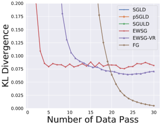
Algorithm 2 EWSG-VR
1:  Input: {number of data terms n𝑛n, gradient functions Vi()subscript𝑉𝑖\nabla V_{i}(\cdot), step size hh, number of data passes K, period of variance calibration L𝐿L, index chain length M𝑀M, friction and noise coefficients γ𝛾\gamma and σ𝜎\sigma}
2:  initialize 𝜽0,𝒓0,γ0=γsubscript𝜽0subscript𝒓0subscript𝛾0𝛾\boldsymbol{\theta}_{0},\boldsymbol{r}_{0},\gamma_{0}=\gamma
3:  initialize inner loop index k=0𝑘0k=0
4:  for l=1,2,,K𝑙12𝐾l=1,2,\cdots,K do
5:     if (l1)modL=0modulo𝑙1𝐿0(l-1)\mod L=0 then
6:        compute 𝒎1𝔼I[nVI(𝜽k)]subscript𝒎1subscript𝔼𝐼delimited-[]𝑛subscript𝑉𝐼subscript𝜽𝑘\boldsymbol{m}_{1}\leftarrow\mathbb{E}_{I}[n\nabla V_{I}(\boldsymbol{\theta}_{k})], 𝒎2𝔼I[n2VI(𝜽k)VI(𝜽k)T]subscript𝒎2subscript𝔼𝐼delimited-[]superscript𝑛2subscript𝑉𝐼subscript𝜽𝑘subscript𝑉𝐼superscriptsubscript𝜽𝑘𝑇\boldsymbol{m}_{2}\leftarrow\mathbb{E}_{I}[n^{2}\nabla V_{I}(\boldsymbol{\theta}_{k})\nabla V_{I}(\boldsymbol{\theta}_{k})^{T}]
7:        𝝎𝜽k𝝎subscript𝜽𝑘\boldsymbol{\omega}\leftarrow\boldsymbol{\theta}_{k}
8:     else
9:        for t=1,2,,nM+1𝑡12𝑛𝑀1t=1,2,\cdots,\lceil\frac{n}{M+1}\rceil do
10:           i𝑖absenti\leftarrow uniformly sampled from 1,,n1𝑛{1,\cdots,n},   compute and store nVi(𝜽k)𝑛subscript𝑉𝑖subscript𝜽𝑘n\nabla V_{i}(\boldsymbol{\theta}_{k})
11:           for m=1,2,,M𝑚12𝑀m=1,2,\cdots,M do
12:              j𝑗absentj\leftarrow uniformly sampled from 1,,n1𝑛{1,\cdots,n},   compute and store nVj(𝜽k)𝑛subscript𝑉𝑗subscript𝜽𝑘n\nabla V_{j}(\boldsymbol{\theta}_{k})
13:              ij𝑖𝑗i\leftarrow j with probability in Equation 6
14:           end for
15:           update (𝜽k+1,𝒓k+1)(𝜽k,𝒓k)subscript𝜽𝑘1subscript𝒓𝑘1subscript𝜽𝑘subscript𝒓𝑘(\boldsymbol{\theta}_{k+1},\boldsymbol{r}_{k+1})\leftarrow(\boldsymbol{\theta}_{k},\boldsymbol{r}_{k}) according to Equation 3, using nVi(𝜽k)𝑛subscript𝑉𝑖subscript𝜽𝑘n\nabla V_{i}(\boldsymbol{\theta}_{k}) as gradient and ΓksubscriptΓ𝑘\Gamma_{k} as friction
16:           𝒎1𝒎1+Vi(𝜽k)Vi(𝝎)subscript𝒎1subscript𝒎1subscript𝑉𝑖subscript𝜽𝑘subscript𝑉𝑖𝝎\boldsymbol{m}_{1}\leftarrow\boldsymbol{m}_{1}+\nabla V_{i}(\boldsymbol{\theta}_{k})-\nabla V_{i}(\boldsymbol{\omega})
17:           𝒎2𝒎2+nVi(𝜽k)Vi(𝜽k)TnVi(𝝎)Vi(𝝎)Tsubscript𝒎2subscript𝒎2𝑛subscript𝑉𝑖subscript𝜽𝑘subscript𝑉𝑖superscriptsubscript𝜽𝑘𝑇𝑛subscript𝑉𝑖𝝎subscript𝑉𝑖superscript𝝎𝑇\boldsymbol{m}_{2}\leftarrow\boldsymbol{m}_{2}+n\nabla V_{i}(\boldsymbol{\theta}_{k})\nabla V_{i}(\boldsymbol{\theta}_{k})^{T}-n\nabla V_{i}(\boldsymbol{\omega})\nabla V_{i}(\boldsymbol{\omega})^{T}
18:           covar𝒎2𝒎1𝒎1Tcovarsubscript𝒎2subscript𝒎1superscriptsubscript𝒎1𝑇\mbox{covar}\leftarrow\boldsymbol{m}_{2}-\boldsymbol{m}_{1}\boldsymbol{m}_{1}^{T}
19:           Γk+112T(σ2I+hcovar)subscriptΓ𝑘112𝑇superscript𝜎2Icovar\Gamma_{k+1}\leftarrow\frac{1}{2T}(\sigma^{2}\text{I}+h\,\mbox{covar})
20:           kk+1𝑘𝑘1k\leftarrow k+1
21:        end for
22:     end if
23:  end for
Refer to caption
Figure 4: KL divergence

To demonstrate the performance of EWSG-VR, we reuse the setup of simple Gaussian example in subsection 5.1. As shown in Algorithm 2, the only hyper-parameter of EWSG-VR additional to EWSG is the period of variance calibration, for which we set L=1𝐿1L=1. All other hyper-parameters (e.g. step size hh, friction coefficient γ𝛾\gamma) are set the same as EWSG. We also run underdamped Langevin dynamics with full gradient (FG) using the same hyper-parameters of EWSG. We plot the KL divergence in Figure 4. We see that EWSG-VR further reduces variance and achieves better statistical accuracy measured in KL divergence. Although EWSG-VR periodically use full data set to calibrate variance estimation, it is still significantly faster than the full gradient version. Note that KL divergence of SGLD, pSGLD and SGHMC are too large so that we can not even see them in Figure 4

We also consider applying EWSG-VR to Bayesian logistic regression problems. We run experiments on two standard classification data sets parkinsons 888https://archive.ics.uci.edu/ml/datasets/parkinsons, pima999https://archive.ics.uci.edu/ml/datasets/diabetes from UCI repository [Lichman et al., 2013].
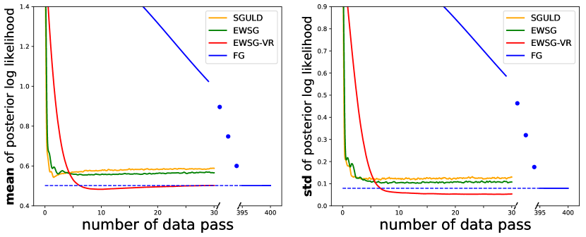
Refer to caption
(a) parkinsons
Refer to caption
(b) pima
Figure 5: Posterior prediction of mean (left) and standard deviation (right) of log likelihood on test data set generated by SGHMC, EWSG and EWSG-VR on two Bayesian logistic regression tasks. Statistics are computed based on 1000 independent simulations. Minibatch size b=1𝑏1b=1 for all methods except FG. M=1𝑀1M=1 for EWSG and EWSG-VR.

From Figure 5, we see stochastic gradient methods (SGHMC, EWSG and EWSG-VR) only take tens of data passes to converge while full gradient version (FG) requires hundreds of data passes to converge. Compared with SGHMC, EWSG produces closer results to FG for which we treat as ground truth, in terms of statistical accuracy. With variance reduction, EWSG-VR is able to achieve even better performance, significantly improving the accuracy of the prediction of mean and standard deviation of log likelihood. It, however, converges slower than EWSG without VR.

One downside of EWSG-VR is that it periodically use whole data set to calibrate variance estimation, so it may not be suitable for very large data sets (e.g. Covertype data set used in subsection 5.2) for which stochastic gradient methods could converge within one data pass.

Appendix G Additional Experiments

G.1 A Misspecified Gaussian Case

In this subsection, we follow the same setup as in [Bardenet et al., 2017] and study a misspecified Gaussian model where one fits a one-dimensional normal distribution p(θ)=𝒩(θ|μ0,σ02)𝑝𝜃𝒩conditional𝜃subscript𝜇0superscriptsubscript𝜎02p(\theta)=\mathcal{N}(\theta|\mu_{0},\sigma_{0}^{2}) to 105superscript10510^{5} i.i.d points drawn according to Xilog𝒩(0,1)similar-tosubscript𝑋𝑖𝒩01X_{i}\sim\log\mathcal{N}(0,1), and flat prior is assigned p(μ0,logσ0)1proportional-to𝑝subscript𝜇0subscript𝜎01p(\mu_{0},\log\sigma_{0})\propto 1. It was shown in [Bardenet et al., 2017] that FlyMC algorithm behaves erratically in this case, as “bright” data points with large values are rarely updated and they drive samples away from the target distribution. Consequently the chain mixes very slowly. One important commonality FlyMC shares with EWSG is that in each iteration, both algorithms select a subset of data in a non-uniform fashion. Therefore, it is interesting to investigate the performance of EWSG in this misspecified model.

For FlyMC101010https://github.com/rbardenet/2017JMLR-MCMCForTallData, a tight lower bound based on Taylor’s expansion is used to minimize “bright” data points used per iteration. At each iteration, 10% data points are resampled and turned “on/off” accordingly and the step size is adaptively adjusted. FlyMC algorithm is run for 10000 iterations. Figure 6(a) shows the histogram of number of data points used in each iteration for FlyMC algorithm. On average, FlyMC consumes 10.9%percent10.910.9\% of all data points per iteration. For fair comparison, the minibatch size of EWSG is hence set 105×10.9%=10900superscript105percent10.91090010^{5}\times 10.9\%=10900 and we run EWSG for 1090 data passes. We set step size h=1×1041superscript104h=1\times 10^{-4} and friction coefficient γ=300𝛾300\gamma=300 for EWSG. An isotropic random walk Metropolis Hastings (MH) is also run for sufficiently long and serves as the ground truth.

Figure 6(b) shows the autocorrelation of three algorithms. The autocorrelation of FlyMC decays very slowly, samples that are even 500 iterations away still show strong correlation. The autocorrelation of EWSG, on the other hand, decays much faster, suggesting EWSG explores parameter space efficiently than FlyMC does. Figure 6(c) and 6(d) show the samples (the first 1000 samples are discarded as burn-in) generated by EWSG and FlyMC respectively. The samples of EWSG center around the mode of the target distribution while the samples of FlyMC are still far away from the true posterior. The experiment shows EWGS works quite well even in misspecified models, and hence is an effective candidate in combining importance sampling with scalable Bayesian inference.
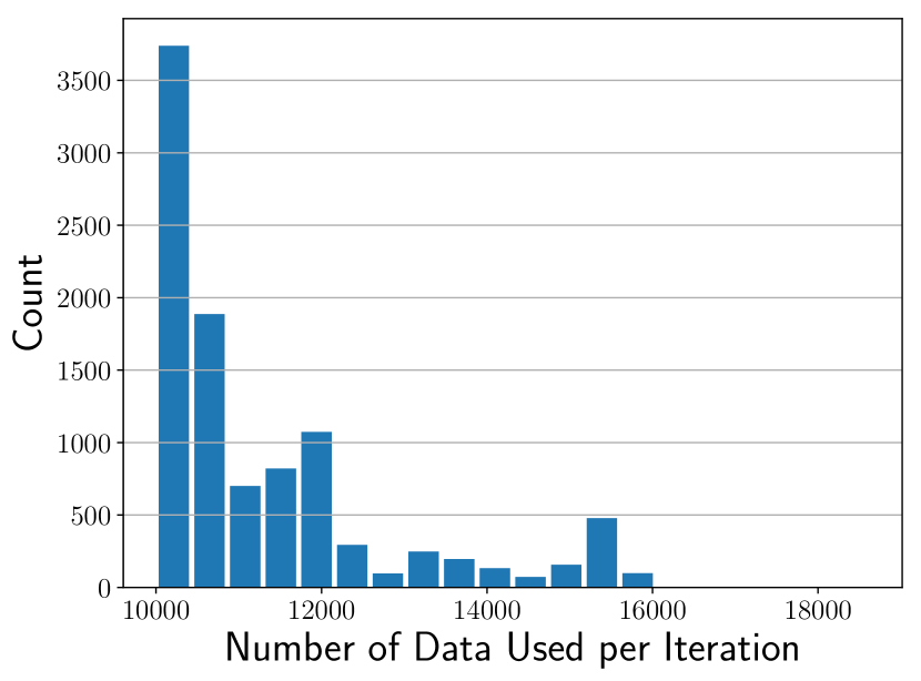
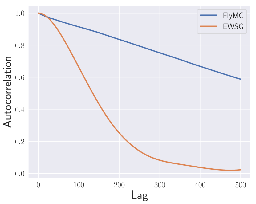
Refer to caption
(a) Histogram
Refer to caption
(b) Autocorrelation
Refer to caption
(c) Samples of EWSG
Refer to caption
(d) Samples of FlyMC
Figure 6: (a) Histogram of data used in each iteration for FlyMC algorithm. (b) Autocorrelation plot of FlyMC, EWSG and MH. (c) Samples of EWSG. (d) Samples of FlyMC.

G.2 Additional Results of BNN Experiment

We report the test error of various SG-MCMC methods after 200 epochs in Table 2. For both MLP and CNN architecture, EWSG outperforms its uniform counterpart SGHMC as well as other benchmarks SGLD, pSGLD and CP-SGHMC. The results clearly demonstrate the effectiveness of the proposed EWSG on deep models.

Table 2: Test error (mean ±plus-or-minus\pm standard deviation) after 200 epoches.
  Method Test Error(%), MLP Test Error(%), CNN
SGLD 1.976 ±plus-or-minus\pm 0.055 0.848 ±plus-or-minus\pm 0.060
pSGLD 1.821 ±plus-or-minus\pm 0.061 0.860 ±plus-or-minus\pm 0.052
SGHMC 1.833 ±plus-or-minus\pm 0.073 0.778 ±plus-or-minus\pm 0.040
CP-SGHMC 1.835 ±plus-or-minus\pm 0.047 0.772 ±plus-or-minus\pm 0.055
EWSG 1.793 ±plus-or-minus\pm 0.100 0.753 ±plus-or-minus\pm 0.035
 

G.3 Additional Experiment on BNN: Tuning M𝑀M

In each iteration of EWSG, we run an index Markov chain of length M𝑀M and select a “good” minibatch to estimate gradient, therefore EWSG essentially uses b×(M+1)𝑏𝑀1b\times(M+1) data points per iteration where b𝑏b is minibatch size. How does EWSG compare with its uniform gradient subsampling counterpart with a larger minibatch size (b×(M+1)𝑏𝑀1b\times(M+1))?

We empirically answer this question in the context of BNN with MLP architecture. We use the same step size for SGHMC and EWSG and experiment a large range of values of minibatch size b𝑏b and index chain length M𝑀M. Each algorithm is run for 200 data passes and 10 independent samples are drawn to estimate test error. The results are shown in Table 3. We find that EWSG beats SGHMC with larger minibatch in 8 out of 9 comparison groups, which suggests in general EWSG could be a better way to consuming data compared to increasing minibatch size and may shed light on other areas where stochastic gradient methods are used (e.g. optimization).

b𝑏b M+1=2𝑀12M+1=2 M+1=5𝑀15M+1=5 M+1=10𝑀110M+1=10
100100100 1.86% 1.94% 1.83% 1.92% 1.80% 1.97%
200200200 1.90% 1.87% 1.87% 1.97% 1.80% 2.07%
500500500 1.79% 1.97% 2.01% 2.17% 2.36% 2.37%

Table 3: Test errors of EWSG (top of each cell) and SGHMC (bottom of each cell) after 200 epoches. b𝑏b is minibatch size for EWSG, and minibatch size of SGHMC is set as b×(M+1)𝑏𝑀1b\times(M+1) to ensure the same number of data used per parameter update for both algorithms. Step size is set h=10b(M+1)10𝑏𝑀1h=\frac{10}{b(M+1)} as suggested in [Chen et al., 2014], different from that used to produce Table 2. Results with smaller test error is highlighted in boldface.

Appendix H EWSG does not necessarily change the speed of convergence significantly

Changing the weights of stochastic gradient from uniform to non-uniform, as we saw, can increase the statistical accuracy of the sampling; however, it does not necessarily increase or decrease the speed of convergence to the (altered) limiting distribution. Numerical examples already demonstrated this fact, but on the theoretical side, we note the non-asymptotic bound provided by Theorem 3 may not be tight in terms of the speed of convergence due to its generality. Therefore, here we quantify the convergence speed on a simple quadratic example:

Consider Vi(θ)=1n(θμi)2/2subscript𝑉𝑖𝜃1𝑛superscript𝜃subscript𝜇𝑖22V_{i}(\theta)=\frac{1}{n}(\theta-\mu_{i})^{2}/2 where μisubscript𝜇𝑖\mu_{i}’s are constant scalars. Assume without loss of generality that iμi=0subscript𝑖subscript𝜇𝑖0\sum_{i}\mu_{i}=0, and thus V(θ)=i=1nVi(θ)=θ2/2+some constant𝑉𝜃superscriptsubscript𝑖1𝑛subscript𝑉𝑖𝜃superscript𝜃22some constantV(\theta)=\sum_{i=1}^{n}V_{i}(\theta)=\theta^{2}/2+\text{some constant}. We will show the convergence speed of 𝔼θ𝔼𝜃\mathbb{E}\theta is comparable for uniform and a class of non-uniform SG-MCMC (including EWSG) applied to second-order Langevin equation (overdamped Langevin will be easier and thus omitted):

Theorem 5

Consider, for 0<γ<20𝛾20<\gamma<2, respectively SGHMC and EWSG,

{θk+1=θk+hrkrk+1=rkhγrkh(θkμIk)+hσξk+1casessubscriptsuperscript𝜃𝑘1absentsubscriptsuperscript𝜃𝑘subscriptsuperscript𝑟𝑘subscriptsuperscript𝑟𝑘1absentsubscriptsuperscript𝑟𝑘𝛾subscriptsuperscript𝑟𝑘subscriptsuperscript𝜃𝑘subscript𝜇subscriptsuperscript𝐼𝑘𝜎subscriptsuperscript𝜉𝑘1\begin{cases}\theta^{\prime}_{k+1}&=\theta^{\prime}_{k}+hr^{\prime}_{k}\\ r^{\prime}_{k+1}&=r^{\prime}_{k}-h\gamma r^{\prime}_{k}-h(\theta^{\prime}_{k}-\mu_{I^{\prime}_{k}})+\sqrt{h}\sigma\xi^{\prime}_{k+1}\end{cases}

and

{θk+1=θk+hrkrk+1=rkhγrkh(θkμIk)+hσξk+1,casessubscript𝜃𝑘1absentsubscript𝜃𝑘subscript𝑟𝑘subscript𝑟𝑘1absentsubscript𝑟𝑘𝛾subscript𝑟𝑘subscript𝜃𝑘subscript𝜇subscript𝐼𝑘𝜎subscript𝜉𝑘1\begin{cases}\theta_{k+1}&=\theta_{k}+hr_{k}\\ r_{k+1}&=r_{k}-h\gamma r_{k}-h(\theta_{k}-\mu_{I_{k}})+\sqrt{h}\sigma\xi_{k+1}\end{cases},

where Iksubscriptsuperscript𝐼𝑘I^{\prime}_{k} are i.i.d. uniform random variable on [n]delimited-[]𝑛[n], Iksubscript𝐼𝑘I_{k} are [θ,r]𝜃𝑟[\theta,r] dependent random variable on [n]delimited-[]𝑛[n] satisfying (Ik=i)=1/n+𝒪(hp)subscript𝐼𝑘𝑖1𝑛𝒪superscript𝑝\mathbb{P}(I_{k}=i)=1/n+\mathcal{O}(h^{p}), and ξk+1,ξk+1subscript𝜉𝑘1subscriptsuperscript𝜉𝑘1\xi_{k+1},\xi^{\prime}_{k+1} are standard i.i.d. Gaussian random variables. Denote by θ¯k=𝔼θksubscript¯superscript𝜃𝑘𝔼subscriptsuperscript𝜃𝑘\bar{\theta^{\prime}}_{k}=\mathbb{E}\theta^{\prime}_{k}, r¯k=𝔼rksubscript¯superscript𝑟𝑘𝔼subscriptsuperscript𝑟𝑘\bar{r^{\prime}}_{k}=\mathbb{E}r^{\prime}_{k}, θ¯k=𝔼θksubscript¯𝜃𝑘𝔼subscript𝜃𝑘\bar{\theta}_{k}=\mathbb{E}\theta_{k}, r¯k=𝔼rksubscript¯𝑟𝑘𝔼subscript𝑟𝑘\bar{r}_{k}=\mathbb{E}r_{k}, xk=[θ¯k,r¯k]Tsubscriptsuperscript𝑥𝑘superscriptsubscript¯superscript𝜃𝑘subscript¯superscript𝑟𝑘𝑇x^{\prime}_{k}=[\bar{\theta^{\prime}}_{k},\bar{r^{\prime}}_{k}]^{T}, and xk=[θ¯k,r¯k]Tsubscript𝑥𝑘superscriptsubscript¯𝜃𝑘subscript¯𝑟𝑘𝑇x_{k}=[\bar{\theta}_{k},\bar{r}_{k}]^{T}, then

xk=(I+Ah)kx0,where A=[011γ],formulae-sequencesubscriptsuperscript𝑥𝑘superscript𝐼𝐴𝑘subscriptsuperscript𝑥0where 𝐴matrix011𝛾x^{\prime}_{k}=(I+Ah)^{k}x^{\prime}_{0},\quad\text{where }A=\begin{bmatrix}0&1\\ -1&-\gamma\end{bmatrix}, (14)

for small enough hh, xknormsubscriptsuperscript𝑥𝑘\|x^{\prime}_{k}\| converges to 0 exponentially with k𝑘k\rightarrow\infty, and xksubscript𝑥𝑘x_{k} converges at a comparable speed in the sense that xkxk=𝒪(hp)normsubscript𝑥𝑘subscriptsuperscript𝑥𝑘𝒪superscript𝑝\|x_{k}-x^{\prime}_{k}\|=\mathcal{O}(h^{p}) if x0=x0subscript𝑥0subscriptsuperscript𝑥0x_{0}=x^{\prime}_{0}.

Proof: Taking the expectation of the [θ,r]superscript𝜃superscript𝑟[\theta^{\prime},r^{\prime}] iteration and using the fact that iμi=0subscript𝑖subscript𝜇𝑖0\sum_{i}\mu_{i}=0 and hence 𝔼μIk=0𝔼subscript𝜇subscriptsuperscript𝐼𝑘0\mathbb{E}\mu_{I^{\prime}_{k}}=0, one easily obtains (14). The geometric convergence of xksubscriptsuperscript𝑥𝑘x^{\prime}_{k} thus follows from the fact that eigenvalues of I+Ah𝐼𝐴I+Ah have less than 1 modulus for small enough hh.

Let ek=[0,𝔼μIk]Tsubscript𝑒𝑘superscript0𝔼subscript𝜇subscript𝐼𝑘𝑇e_{k}=[0,\mathbb{E}\mu_{I_{k}}]^{T} and then

ek=[0,i=1n(Ik=i)μi]T=[0,𝒪(hp)]Tsubscript𝑒𝑘superscript0superscriptsubscript𝑖1𝑛subscript𝐼𝑘𝑖subscript𝜇𝑖𝑇superscript0𝒪superscript𝑝𝑇e_{k}=[0,\sum_{i=1}^{n}\mathbb{P}(I_{k}=i)\mu_{i}]^{T}=[0,\mathcal{O}(h^{p})]^{T}

Now we take the expectation of both sides of the [θ,r]𝜃𝑟[\theta,r] iteration and obtain xk+1=(I+Ah)xk+heksubscript𝑥𝑘1𝐼𝐴subscript𝑥𝑘subscript𝑒𝑘x_{k+1}=(I+Ah)x_{k}+he_{k}. Therefore

xk=subscript𝑥𝑘absent\displaystyle x_{k}= (I+Ah)kx0+(I+Ah)k1he0++(I+Ah)hek2+hek1superscript𝐼𝐴𝑘subscript𝑥0superscript𝐼𝐴𝑘1subscript𝑒0𝐼𝐴subscript𝑒𝑘2subscript𝑒𝑘1\displaystyle(I+Ah)^{k}x_{0}+(I+Ah)^{k-1}he_{0}+\cdots+(I+Ah)he_{k-2}+he_{k-1}
=\displaystyle= xk+h((I+Ah)k1e0++(I+Ah)ek2+ek1)subscriptsuperscript𝑥𝑘superscript𝐼𝐴𝑘1subscript𝑒0𝐼𝐴subscript𝑒𝑘2subscript𝑒𝑘1\displaystyle x^{\prime}_{k}+h\big{(}(I+Ah)^{k-1}e_{0}+\cdots+(I+Ah)e_{k-2}+e_{k-1}\big{)}

To bound the difference, note I+Ah𝐼𝐴I+Ah is diagonalizable with complex eigenvalues λ1,2subscript𝜆12\lambda_{1,2} satisfying

|λ1|=|λ2|=1hγ+h2=1γh/2+𝒪(h2).subscript𝜆1subscript𝜆21𝛾superscript21𝛾2𝒪superscript2|\lambda_{1}|=|\lambda_{2}|=\sqrt{1-h\gamma+h^{2}}=1-\gamma h/2+\mathcal{O}(h^{2}).

Projecting ejsubscript𝑒𝑗e_{j} to the corresponding eigenspaces via ej=v1,j+v2,jsubscript𝑒𝑗subscript𝑣1𝑗subscript𝑣2𝑗e_{j}=v_{1,j}+v_{2,j}, we can get

h(I+Ah)k1e0++ek1normsuperscript𝐼𝐴𝑘1subscript𝑒0subscript𝑒𝑘1\displaystyle h\|(I+Ah)^{k-1}e_{0}+\cdots+e_{k-1}\| h((I+Ah)k1e0++ek1)absentnormsuperscript𝐼𝐴𝑘1subscript𝑒0normsubscript𝑒𝑘1\displaystyle\leq h\left(\|(I+Ah)^{k-1}e_{0}\|+\cdots+\|e_{k-1}\|\right)
=h(|λ1|k1v1,0+|λ2|k1v2,0++v1,k1+v2,k1)absentsuperscriptsubscript𝜆1𝑘1normsubscript𝑣10superscriptsubscript𝜆2𝑘1normsubscript𝑣20normsubscript𝑣1𝑘1normsubscript𝑣2𝑘1\displaystyle=h\left(|\lambda_{1}|^{k-1}\|v_{1,0}\|+|\lambda_{2}|^{k-1}\|v_{2,0}\|+\cdots+\|v_{1,k-1}\|+\|v_{2,k-1}\|\right)
hChp(|λ1|k1++1)=hChp1|λ1|k1|λ1|hChp11|λ1|absent𝐶superscript𝑝superscriptsubscript𝜆1𝑘11𝐶superscript𝑝1superscriptsubscript𝜆1𝑘1subscript𝜆1𝐶superscript𝑝11subscript𝜆1\displaystyle\leq hCh^{p}(|\lambda_{1}|^{k-1}+\cdots+1)=hCh^{p}\frac{1-|\lambda_{1}|^{k}}{1-|\lambda_{1}|}\leq hCh^{p}\frac{1}{1-|\lambda_{1}|}
C^hpabsent^𝐶superscript𝑝\displaystyle\leq\hat{C}h^{p}

for some constant C𝐶C and C^^𝐶\hat{C}.  

Important to note is, although this is already a nonlinear example for EWSG (as nonlinearity enters through the μIksubscript𝜇subscript𝐼𝑘\mu_{I_{k}} term), it is a linear example for SGHMC. For the fully nonlinear cases, a tight quantification of EWSG’s convergence speed remains to be an open theoretical challenge (a loose quantification is already given by the general Theorem 3).