On rectangle-decomposable 2-parameter persistence modules

Abstract

This paper addresses two questions: (a) can we identify a sensible class of 2-parameter persistence modules on which the rank invariant is complete? (b) can we determine efficiently whether a given 2-parameter persistence module belongs to this class? We provide positive answers to both questions, and our class of interest is that of rectangle-decomposable modules. Our contributions include: on the one hand, a proof that the rank invariant is complete on rectangle-decomposable modules, together with an inclusion-exclusion formula for counting the multiplicities of the summands; on the other hand, algorithms to check whether a module induced in homology by a bifiltration is rectangle-decomposable, and to decompose it in the affirmative, with a better complexity than state-of-the-art decomposition methods for general 2-parameter persistence modules. Our algorithms are backed up by a new structure theorem, whereby a 2-parameter persistence module is rectangle-decomposable if, and only if, its restrictions to squares are. This local characterization is key to the efficiency of our algorithms, and it generalizes previous conditions derived for the smaller class of block-decomposable modules. It also admits an algebraic formulation that turns out to be a weaker version of the one for block-decomposability. By contrast, we show that general interval-decomposability does not admit such a local characterization, even when locality is understood in a broad sense. Our analysis focuses on the case of modules indexed over finite grids, the more general cases are left as future work.

1 Introduction

A persistence module $M$ over a subset $U\subseteq{\mathbb{R}}^{d}$ is a collection of vector spaces $\{M_{t}\}_{t\in U}$ and linear maps ${\rho}_{s}^{t}:=M(s\leq t)\colon M_{s}\to M_{t}$ with the property that ${\rho}_{s}^{s}$ is the identity map and ${\rho}_{t}^{u}\circ{\rho}_{s}^{t}={\rho}_{s}^{u}$ for all $s\leq t\leq u\in U$. Here $s\leq t$ if and only if $s_{i}\leq t_{i}$ for all $i\in\{1,2,\ldots,d\}$. In the language of category theory, a persistence module $M$ is a functor $M\colon U\to{\mathsf{vec}}$ where ${\mathsf{vec}}$ is the category of vector spaces and the partially ordered set $U$ is considered as a category in the obvious way. In this setting, morphisms between persistence modules are natural transformations $M\Rightarrow N$ between functors, defined by collections of linear maps $\{\varphi_{t}:M_{t}\to N_{t}\}_{t\in U}$ such that $\varphi_{t}\circ M(s\leq t)=N(s\leq t)\circ\varphi_{s}$ for all $s\leq t\in U$. Their kernels, images and cokernels, as well as products, direct sums and quotients of persistence modules, are defined pointwise at each index $t\in U$. Similarly, an isomorphism between two persistence modules is a natural isomorphism between them. We will refer to the case $d=1$ as single-parameter persistence, and for $d\geq 2$ we will use the term multi-parameter persistence.

Remark 1.1.

Throughout this paper we will work exclusively with finite-dimensional vector spaces over a fixed field k. When finite-dimensionality is emphasized we will refer to the persistence module as being pointwise finite-dimensional (pfd).

Single-parameter persistence modules are typically obtained through the application of homology to a filtered topological space. This process is known as persistent homology and has found a wide range of applications to the sciences, as well as to other parts of mathematics such as symplectic geometry. See [16, 23] for an introduction to persistent homology. What makes such persistence modules particularly amenable to data analysis is that they can be completely described by multisets of intervals in ${\mathbb{R}}$ called barcodes [14]. Such a collection of intervals can then in turn be used to extract topological information from the data at hand, and further utilized in statistics and machine learning. We now give an example of this structure theorem in the simple case of $U=\{1,2,3\}\subseteq{\mathbb{R}}$.

Example 1.2.

Consider the following sequence of vector spaces and linear maps

$$\textnormal{{k}}^{2}\xrightarrow{\begin{bmatrix}1&1\\ 0&1\end{bmatrix}}\textnormal{{k}}^{2}\xrightarrow{[1~{}-1]}\textnormal{{k}}.$$

By replacing the basis $\{e_{1},e_{2}\}$ of the middle vector space $\textnormal{{k}}^{2}$ with the basis $\{e_{1},e_{1}+e_{2}\}$ we get the following matrix representations of the linear maps

$$\textnormal{{k}}^{2}\xrightarrow{\begin{bmatrix}1&0\\ 0&1\end{bmatrix}}\textnormal{{k}}^{2}\xrightarrow{[1~{}0]}\textnormal{{k}}=\left(\textnormal{{k}}\xrightarrow{1}\textnormal{{k}}\xrightarrow{1}\textnormal{{k}}\right)\oplus\left(\textnormal{{k}}\xrightarrow{1}\textnormal{{k}}\to 0\right).$$

The two persistence modules on the right-hand side are uniquely specified by their supports $\{1,2,3\}$ and $\{1,2\}$, respectively. Their supports give rise to the barcode which in this case is given by $\{\{1,2,3\},\{1,2\}\}$.

As illustrated by ex:1D, a persistence module can be recovered from its barcode thanks to the notion of indicator modules: for $X\times Y\subseteq{\mathbb{R}}^{2}$ and a subset $Q\subseteq X\times Y$, the indicator module of $Q$, denoted $\textnormal{{k}}_{Q}$, is defined by

$$\textnormal{{k}}_{Q,t}=\begin{cases}\textnormal{{k}}&(t\in Q)\\ 0&(t\notin Q)\end{cases} \textnormal{{k}}_{Q}(s\leq t)=\begin{cases}\textnormal{Id}_{\textnormal{{k}}}&\mbox{ if }s\mbox{ and }t\in Q,\\ 0&\mbox{ else}.\end{cases}$$

By convention, we set $\textnormal{{k}}_{\emptyset}={\mathsf{0}}$. A persistence module is an interval module if it is the indicator module of an interval. Note that, just as choosing a basis for a vector space is not canonical, there may be many ways of decomposing a single-parameter persistence module into a direct sum of such interval modules. However, just as for the dimension of a finite-dimensional vector space, the associated barcode given by the multiset of interval supports of the summands is independent of the chosen decomposition [1].

Another desirable property of single-parameter persistence modules $M$ is that they are completely described up to isomorphism by the rank invariant, i.e. the collection of ranks $r(s,t)=\textnormal{rank}(M(s\leq t))$ for all $s\leq t$. This can easily be verified in the previous example, and more generally, for any pfd persistence module $M$ indexed over a finite set $\llbracket 1,n\rrbracket$, the following inclusion-exclusion formula (also known as the persistence measure [10, 12]) gives the multiplicity $m(s,t)$ of any interval $\llbracket s,t\rrbracket$ in the barcode of $M$:

$$m(s,t)=r(s,t)-r(s-1,t)-r(s,t+1)+r(s-1,t+1).$$ (1)

Many applications do however naturally come equipped with multiple parameters, and for such applications it is natural to consider multi-parameter persistence modules, see e.g. the introduction of [2] for an example of how multi-parameter persistence connects to hierarchical clustering. Let us first consider the simplest instantiation of 2-parameter persistence modules, namely modules indexed by the square $S=\{a=(0,0),b=(1,0),c=(0,1),d=(1,1)\}\subseteq{\mathbb{R}}^{2}$.

Example 1.3.

The persistence module on the left-hand side below can be transformed into the one on the right-hand side via a change of basis at the vertices:

In turn, the persistence module on the right-hand side is the direct sum

$$\leavevmode\hbox to69.9pt{\vbox to58.03pt{\text{[drawing]}}}\quad\oplus\quad\leavevmode\hbox to69.9pt{\vbox to58.53pt{\text{[drawing]}}} {0} {0} \scriptstyle{1} \scriptstyle{0} \scriptstyle{0} \scriptstyle{0} \scriptstyle{1} \scriptstyle{1} \scriptstyle{1} \scriptstyle{1} {0} {0} \scriptstyle{1} \scriptstyle{0} \scriptstyle{0} \scriptstyle{0} \scriptstyle{1} \scriptstyle{1} \scriptstyle{1} \scriptstyle{1}$$

Just as in ex:1D, these persistence modules are completely defined by their support. We define the barcode of the aforementioned persistence module to be the (multi-)set of supports of its summands, namely $\{\{c,d\},\{a,b,c,d\}\}$.

Although commutative diagrams like the one in the previous example may appear unwieldy at first glance, such persistence modules can — just as in the single-parameter case — be completely described (up to isomorphism) by a multiset of elements from

$$\mathcal{I}:=\{\{a\},\{b\},\{c\},\{d\},\{a,b\},\{a,c\},\{b,d\},\{c,d\},\{a,b,c\},\{b,c,d\},\{a,b,c,d\}\},$$ (2)

called intervals in the $2\times 2$ grid. See e.g. Figure 13 in [17]. However, in contrast to the single-parameter case, the rank invariant on persistence modules indexed by $S$ is no longer a complete invariant, i.e. it does not fully determine the isomorphism type of such modules. For instance, two persistence modules with barcodes $\{\{a,b,c\},\{a\}\}$ and $\{\{a,b\},\{\{a,c\}\}$ are non-isomorphic yet exhibit the same rank invariant.

Example 1.4.

Consider the following two persistence modules:

The diagram to the left can easily be seen to be composed of two interval summands in the $3\times 2$ grid. By contrast, the diagram to the right is indecomposable: there exists no change of basis for which this persistence module can be written as a direct sum of persistence modules in a non-trivial way. Again, the two modules have the same rank invariant.

In the setting of no more than four columns and two rows, results from the field of representation theory of quivers show that there exists a finite set of building blocks (indecomposable modules) from which every persistence module can be built (via direct sums, and up to isomorphism). Based on this, one can associate a well-defined barcode-like structure to such a module by counting the multiplicity of every summand in the decomposition. The inclusion of such grids into topological data analysis was inspired by a problem in materials science [17]. For five or more columns the theory becomes increasingly complex. In particular, for six or more columns there is no way to parametrize a set of building blocks in any reasonable way. This is a major obstacle to the development of the theory of multi-parameter persistence.

A natural question to consider then is whether one can endow multi-parameter persistence modules with additional structure in order to enforce nice decomposition theorems akin to that of single-parameter persistence. One such setting coming from computational topology was identified in [3, 9], and further generalized in [11], where it is shown that the so-called strongly exact 2-parameter persistence modules indexed over ${\mathbb{R}}^{2}$ are determined (up to isomorphism) by a multiset of particularly simple planar rectangular regions called blocks. Basically, a block is either an upper-right or lower-left quadrant, or a horizontal or vertical infinite band. The great advantage of this condition is that it can be checked locally: a 2-parameter persistence module (called a bimodule for short) is block-decomposable if, and only if, its restriction to any square as in Example 1.3 is block-decomposable.

Contributions. In this paper we address two important follow-up questions:

• Can we work out conditions such as above for larger classes of bimodules?

• Can we identify classes of bimodules for which the rank invariant is complete?

Our answers to both questions are positive, and the two classes of bimodules turn out to be the same, namely that of rectangle-decomposable bimodules, which by definition are determined (up to isomorphism) by a multiset of rectangles, i.e subsets $R$ of the form $R=I\times J\subseteq{\mathbb{R}}^{2}$ where $I$ and $J$ are intervals in ${\mathbb{R}}$. Specifically, a bimodule is rectangle-decomposable if it decomposes into a direct sum of rectangle modules, i.e. indicator modules of rectangles.

Our local condition for rectangle decomposability, called weak exactness, is a weaker version of the condition for block decomposability, in that it allows all types of rectangular shapes in the local squares’ decompositions, as opposed to just blocks. More precisely, calling $\mathcal{R}$ the following subset of $\mathcal{I}$:

$$\mathcal{R}=\{\{a\},\{b\},\{c\},\{d\},\{a,b\},\{a,c\},\{b,d\},\{c,d\},\{a,b,c,d\}\},$$ (3)

Definition 1.5 (Weak exactness).

Given subsets $X,Y$ of ${\mathbb{R}}$, a persistence module $M\colon X\times Y\subseteq{\mathbb{R}}\times{\mathbb{R}}\to{\mathsf{vec}}$ is weakly exact if the barcode of the following square

(4)

consists of elements from $\mathcal{R}$ for all indices $s\leq t$ in $X\times Y$.

By comparison, the strong exactness condition replaces $\mathcal{R}$ by $\mathcal{B}=\mathcal{R}\setminus\{\{b\},\{c\}\}$.

Example 1.6.

The persistence module to the left below is strongly exact, while the one to the right is only weakly exact, and the persistence modules in ex:3-2-indecomposable are not even weakly exact (each time the weak or strong exactness condition fails on the outermost rectangle):

Our analysis focuses on the case of modules indexed over finite grids, the more general cases are left as future work. Our contributions summarize as follows:

• In Section 2 we prove that the rank invariant is complete on the class of rectangle-decomposable bimodules (Theorem 2.1). To this end, we generalize the inclusion-exclusion formula (1) to our setting. Note that our result also follows indirectly from an inclusion-exclusion formula for a generalization of the rank invariant for interval-decomposable modules [19, Prop. 7.13], but that we provide an explicit statement together with a simple and direct proof.

• In Section 3 we show that the rank invariant of a simplicial bifiltration with a total of $n$ simplices can be computed in $O(n^{4})$ time (Theorem 3.1). This result in itself is not new, however, combined with our inclusion-exclusion formula, it yields an $O(n^{4})$ time algorithm for computing the barcode of a persistence bimodule that is known to be rectangle-decomposable (Corollary 3.2). This is an improvement over merely applying some state-of-the-art algorithm for computing decompositions of general 2-parameter persistence modules, which would take $O(n^{2\omega+1})$ time where $2\leq\omega<2.373$ is the exponent for matrix multiplication [15].

• In Section 4 we propose an algebraic formulation of our weak exactness condition (def:weak-exactness-alg). This formulation turns out to be equivalent to def:weak-exactness-geom and to global rectangle-decomposability (the central mathematical result in the paper), specifically:

  Theorem 1.7.

  Let $M$ be a pfd persistence module indexed over $X\times Y$, where $X,Y$ are finite subsets of ${\mathbb{R}}$. Then, $M$ is rectangle-decomposable if and only if $M$ is weakly exact.

• In Section 5 we leverage this result to derive an $O(n^{2+\omega})$-time algorithm for checking the rectangle-decomposability of persistence bimodules induced in homology from simplicial bifiltrations with at most $n$ simplices (Theorem 5.1). Once again, this is an improvement over applying some state-of-the-art algorithm for computing decompositions of general 2-parameter persistence modules and then checking the summands one by one.

• In Section 6 we investigate the existence of similar local characterizations for larger classes of interval-decomposable modules. First, we show that interval-decomposability itself cannot be characterized locally, even when testing on arbitrary strict subgrids and not just squares. Second, we show that decomposability with respect to certain classes of indecomposables in-between the rectangle modules and the interval modules cannot be characterized locally either when testing on squares.

• Finally, in Section 7 we show how rectangle-decomposable modules arise from (sufficiently tame) real-valued functions on a topological space. This is then used to give a new proof of the pyramid basis theorem of [3].

2 Completeness of the rank invariant

Suppose in this section that $X,Y$ are subsets of ${\mathbb{Z}}$.

Theorem 2.1.

The isomorphism type of any pfd rectangle-decomposable persistence module $M$ over $X\times Y$ is fully determined by the rank invariant of $M$.

The proof consists in showing that the multiplicity $m(s,t)$ of each individual rectangle module $\textnormal{{k}}_{\llbracket s_{x},t_{x}\rrbracket\times\llbracket s_{y},t_{y}\rrbracket}$ in the decomposition of $M$ is given by the inclusion-exclusion formula (7) below, which involves only the rank invariant $r:(X\times Y)^{2}\to{\mathbb{N}}$ of $M$ — with the convention that $r(s,t)=0$ whenever $s\nleq t$. This formula is the analogue, in the category of rectangle-decomposable pfd bimodules, of the inclusion-exclusion formula (1) for counting the multiplicities of interval summands in one-parameter persistence.

Fix arbitrary indices $s\leq t\in X\times Y$. Recall that the rank of $(A\oplus B)(s\leq t)$ is equal to the sum of the ranks of $A(s\leq t)$ and $B(s\leq t)$. Meanwhile, for any summand $\textnormal{{k}}_{R}$ of $M$, the rank of $\textnormal{{k}}_{R}(s\leq t)$ is $1$ if $s,t\in R$ and $0$ otherwise. Therefore, $r(s,t)$ counts (with multiplicity) the number of summands of $M$ whose rectangle support contains both $s$ and $t$. Then, denoting by $m(s,t^{+})$ the number of (rectangle) summands whose support contains $t$ and has $s$ as lower-left corner, we have the folllowing inclusion-exclusion formula:

$$m(s,t^{+})=r(s,t)-r((s_{x}-1,s_{y}),t)-r((s_{x},s_{y}-1),t)+r((s_{x}-1,s_{y}-1),t).$$ (5)

This formula can be interpreted as follows: a rectangle containing $t$ has $s$ as lower-left corner if and only if it contains $s$ but neither $(s_{x}-1,s_{y})$ nor $(s_{x},s_{y}-1)$; and it contains both $(s_{x}-1,s_{y})$ and $(s_{x},s_{y}-1)$ if and only if it contains $(s_{x}-1,s_{y}-1)$.

Using the same approach at $t$, we can now compute the number $m(s,t)$ of summands of $M$ whose support has $s$ as lower-left corner and $t$ as upper-right corner (i.e. is the rectangle $\llbracket s_{x},t_{x}\rrbracket\times\llbracket s_{y},t_{y}\rrbracket$). The corresponding inclusion-exclusion formula is:

$$m(s,t)=m(s,t^{+})-m(s,(t_{x}+1,t_{y})^{+})-m(s,(t_{x},t_{y}+1)^{+})+m(s,(t_{x}+1,t_{y}+1)^{+}).$$ (6)

Combining (5) and (6) together gives the desired inclusion-exclusion formula for the multiplicity $m(s,t)$ of the summand $\textnormal{{k}}_{\llbracket s_{x},t_{x}\rrbracket\times\llbracket s_{y},t_{y}\rrbracket}$ in the decomposition of $M$ from the rank invariant, hence completing the proof of Theorem 2.1, namely:

$$\begin{gathered}\begin{array}[]{rcl}m(s,t)&=&r(s,t)-r((s_{x}-1,s_{y}),t)\\[5.0pt] &&\hskip 10.0pt-r((s_{x},s_{y}-1),t)+r((s_{x}-1,s_{y}-1),t)\\[5.0pt] &&-r(s,(t_{x}+1,t_{y}))+r((s_{x}-1,s_{y}),(t_{x}+1,t_{y}))\\[5.0pt] &&\hskip 10.0pt+r((s_{x},s_{y}-1),(t_{x}+1,t_{y}))-r((s_{x}-1,s_{y}-1),(t_{x}+1,t_{y}))\\[5.0pt] &&-r(s,(t_{x},t_{y}+1))+r((s_{x}-1,s_{y}),(t_{x},t_{y}+1))\\[5.0pt] &&\hskip 10.0pt+r((s_{x},s_{y}-1),(t_{x},t_{y}+1))-r((s_{x}-1,s_{y}-1),(t_{x},t_{y}+1))\\[5.0pt] &&+r(s,(t_{x}+1,t_{y}+1))-r((s_{x}-1,s_{y}),(t_{x}+1,t_{y}+1))\\[5.0pt] &&\hskip 10.0pt-r((s_{x},s_{y}-1),(t_{x}+1,t_{y}+1))+r((s_{x}-1,s_{y}-1),(t_{x}+1,t_{y}+1)).\end{array}\end{gathered}$$ (7)

3 Computing the rank invariant and rectangle decompositions

Let $F$ be a simplicial bifiltration with $n$ simplices in total. Assume without loss of generality that $F$ is indexed over the grid $G=\llbracket 1,n\rrbracket\times\llbracket 1,n\rrbracket$, for any larger indexing grid must contain arrows with identity maps that can be pre- or post-composed, and any smaller grid can be enlarged by inserting arrows with identity maps. Assume further that each arrow $F_{(i,j)}\to F_{(i+1,j)}$ or $F_{(i,j)}\to F_{(i,j+1)}$ is either an identity map or the insertion of a single simplex. We also fix a homology degree $p$.

Theorem 3.1.

Given the above input, the rank invariant of the persistence bimodule $M$ induced by $F$ in $p$-th homology can be computed in $O(n^{4})$ time.

A proof of this result can be found in D. Morozov’s Ph.D. thesis [22, Section 4.4.2]. We reproduce it below for completeness, with a slight adaptation that allows us to avoid assuming that $F$ is 1-critical. Before giving the proof, let us mention that this theorem, combined with the inclusion-exclusion formula (7), gives an $O(n^{4})$-time algorithm to compute the barcode of $F$ assuming that $M$ is rectangle-decomposable: once the rank invariant of $M$ has been computed, iterate over all the pairs $(s,t)$ with $s\leq t\in G$ and, for each one of them, apply the formula in constant time to get the multiplicity of the rectangle module $\textnormal{{k}}_{\llbracket s_{x},t_{x}\rrbracket\times\llbracket s_{y},t_{y}\rrbracket}$ in the decomposition of $M$. Thus,

Corollary 3.2.

Computing the decomposition of a rectangle-decomposable module over $X\times Y$ induced in homology by a bifiltration with $n$ simplices in total can be done in $O(n^{4})$ time.

This complexity compares favorably to that of the currently best known algorithm for computing direct-sum decompositions of general persistence bimodules, which is $O(n^{2\omega+1})$ where $2\leq\omega<2.373$ is the exponent for matrix multiplication [15].

Figure 1: Left: the stair $S_{(i,j)}$. Center: transitioning from $S_{(i,j)}$ to $S_{(i+1,j)}$ via a sequence of $O(n)$ intermediate paths with 2 steps each. Right: transitioning from $S_{(1,j)}$ to $S_{(1,j+1)}$.

Let us now provide the algorithm for Theorem 3.1. First, we provide a simplified algorithm that runs in $O(n^{2+\omega})$ time. Consider all the paths of the form $(1,1)\to\cdots\to(i,1)\to\cdots\to(i,j)\to\cdots\to(n,j)\to\cdots\to(n,n)$ in the $n\times n$ grid, where $(i,j)\in\llbracket 1,n\rrbracket^{2}$ is arbitrary, as illustrated in Figure 1 (left). We call such a path a stair, denoted by $S_{(i,j)}$, and we call the corresponding index $(i,j)$ its nosing. Note that all the stairs whose nosing is of the form $(i,1)$ or $(n,j)$ are in fact identical to the path $(1,1)\to\cdots\to(n,1)\to\cdots\to(n,n)$, while all the other stairs with different nosings are different. The key observation is that, for any pair of comparable indices $(i,j)\leq(i^{\prime},j^{\prime})$, the stair with nosing $(i,j^{\prime})$ passes through both indices. Computing the rank invariant can then be done by iterating over all the stairs, for instance in lexicographical order of the coordinates of their respective nosings, and for each such stair $S_{(i,j)}$, by computing the persistence barcode of the 1-parameter restriction $F|_{S_{(i,j)}}$ and then using this barcode to report the ranks between all the grid indices encountered along the path. This takes $O(n^{\omega})$ per stair, using the 1-parameter persistence algorithm based on fast matrix multiplication [21], and as there are $O(n^{2})$ stairs in total, the overall running time of the algorithm is $O(n^{2+\omega})$.

In order to reduce the overall complexity to $O(n^{4})$, we exploit the additional observation that, to transition between two consecutive stairs in lexicographical order of the coordinates of their nosings, say $S_{(i,j)}$ and $S_{(i+1,j)}$, one can go through a sequence of $O(n)$ intermediate paths of the form $(1,1)\to\cdots\to(i,1)\to\cdots\to(i,k)\to(i+1,k)\to\cdots\to(i+1,j)\to\cdots\to(n,j)\to\cdots\to(n,n)$, where $k$ ranges from $2$ to $j-1$, as illustrated in Figure 1 (center). Any two consecutive paths in this sequence differ only at a single cell of the grid $\llbracket 1,n\rrbracket^{2}$, therefore the restrictions of $F$ to these two paths either do not differ, or differ by one simplex being inserted one step earlier or later, or by two consecutive simplex insertions being exchanged. In any situation, the persistence barcode can be updated in $O(n)$ time using the vineyards algorithm [13]. The update of the barcode from $S_{(i,j)}$ to $S_{(i+1,j)}$ then takes $O(n^{2})$ time. Likewise, we can compute the barcode of $F|_{S_{(1,j+1)}}$ by transitioning from $S_{(1,j)}$ via an intermediate sequence of $O(n)$ paths differing at a single cell in the grid each time, as illustrated in Figure 1 (right). Thus, the barcode of $F|_{S_{(1,j+1)}}$ is also obtained in $O(n^{2})$ time, and so the overall running time of the algorithm is reduced to $O(n^{4})$. This concludes the proof of Theorem 3.1.

ompute a free resolution of $M$ of size $O(n^{2})$ from $F$ in $O(n^{3})$ time using the algorithm of [lesnick2019computing]. This free resolution takes the form of an exact sequence as follows:

where $M_{\gamma}$, $M_{\eta}$ and $M_{\zeta}$ are free bigraded modules, equipped with bases $(\gamma_{1},\cdots,\gamma_{k})$, $(\eta_{1},\cdots,\eta_{l})$, $(\zeta_{1},\cdots,\zeta_{m})$ respectively, of sizes $k,l,m\leq n$. The elements $\gamma_{i}$ are called generators, while the $\eta_{j}$ are called relations and the $\zeta_{r}$ are called relations on relations. Each one of them is homogeneous and thus assigned a unique grade, denoted by $\operatorname{gr}(\cdot)$. The morphisms of free bigraded modules $\varphi$, $\psi$ are given as $k\times l$ and $l\times m$ matrices respectively, with coefficients in k. Exactness implies that $\psi$ is injective and $M\cong\operatorname{Coker}\varphi$.

Ignoring first the relations and the relations on relations (i.e. assuming that $l=m=0$ hence $M_{\eta}=M_{\zeta}=0$), the rank invariant $r:\llbracket 1,n\rrbracket^{2}\times\llbracket 1,n\rrbracket^{2}\to{\mathbb{N}}$ is given by:

$$\forall s\leq t\in G,\quad r(s,t)=\#\{i\mid\operatorname{gr}(\gamma_{i})\leq s\}.$$

Computing the numbers on the right-hand side for all $s\leq t\in G$ is easily done in $O(n^{4})$ time by dynamic programming: first we iterate over the $k\leq n$ generators to fill in an $n\times n$ table storing at each index $s$ the number of generators having $s$ as their grade; then we build a $n^{2}\times n^{2}$ lookup table by iterating over the indices $(s,t)$ in lexicographic order and using the following recurrence formula:

$$\begin{split}\#\{i\mid\operatorname{gr}(\gamma_{i})\leq s\}\quad=&\quad\#\{i\mid\operatorname{gr}(\gamma_{i})<s\}+\#\{i\mid\operatorname{gr}(\gamma_{i})=s\}\\ =&\quad\#\{i\mid\operatorname{gr}(\gamma_{i})\leq(s_{x}-1,s_{y})\}+\#\{i\mid\operatorname{gr}(\gamma_{i})\leq(s_{x},s_{y}-1)\}\\ &\quad-\#\{i\mid\operatorname{gr}(\gamma_{i})\leq(s_{x}-1,s_{y}-1)\}+\#\{i\mid\operatorname{gr}(\gamma_{i})=s\}.\end{split}$$

Once this is done, we can take the relations into account (still ignoring relations on relations, i.e. assuming that $m=0$ hence $M_{\zeta}=0$). Each relation $\eta_{j}$ gives a k-linear constraint on a subset $\Upsilon$ of the generators, encoded in the $j$-th column of the matrix of $\varphi$: $\sum_{u\in\Upsilon}\alpha_{u}\gamma_{u}=0$, where each $\alpha_{u}$ belongs to $\textnormal{{k}}\setminus\{0\}$. Call $\operatorname{lub}(\eta_{j})$ the least upper bound of the set $\{\operatorname{gr}(\gamma_{u})\mid u\in\Upsilon\}$ in the product order $\leq$ on $G$. The effect of $\eta_{j}$ on the rank invariant is to decrement it at indices $s\leq t$ such that $s\geq\operatorname{lub}(\eta_{j})$ and $t\geq\operatorname{gr}(\eta_{j})$, as illustrated in Figure 2. Hence the following formula for the update of $r(s,t)$:

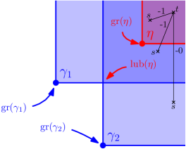
Figure 2: A relation $\eta$ between two generators $\gamma_{1},\gamma_{2}$, and its effect on $r(s,t)$ for various $s\leq t$.

$$r(s,t)\quad\longleftarrow\quad r(s,t)-\#\{j\mid\operatorname{lub}(\eta_{j})\leq s\ \mbox{and}\ \operatorname{gr}(\eta_{j})\leq t\}.$$

The numbers on the right-hand side can be computed in $O(n^{4})$ time again using dynamic programming: first we build a $n^{2}\times n^{2}$ table storing at each index $(s,t)$ the number of relations $\eta_{j}$ such that $\operatorname{gr}(\eta_{j})=t$ and $\operatorname{lub}(\eta_{j})=s$; then for each index $t\in G$ we build an intermediate $n\times n$ lookup table by iterating over the indices $s$ in lexicographic order and using the following recurrence formulaf:formula_special:

$$\begin{split}\#\{j\mid\operatorname{lub}(\eta_{j})\leq s\ \mbox{and}\ \operatorname{gr}(\eta_{j})=t\}\quad=&\#\{j\mid\operatorname{lub}(\eta_{j})\leq(s_{x}-1,s_{y})\ \mbox{and}\ \operatorname{gr}(\eta_{j})=t\}\\ &+\#\{j\mid\operatorname{lub}(\eta_{j})\leq(s_{x},s_{y}-1)\ \mbox{and}\ \operatorname{gr}(\eta_{j})=t\}\\ &-\#\{j\mid\operatorname{lub}(\eta_{j})\leq(s_{x}-1,s_{y}-1)\ \mbox{and}\ \operatorname{gr}(\eta_{j})=t\}\\ &+\#\{j\mid\operatorname{lub}(\eta_{j})=s\ \mbox{and}\ \operatorname{gr}(\eta_{j})=t\};\end{split}$$

finally, we build the lookup table for the rank invariant $r$ by iterating over the indices $(s,t)$ in lexicographic order and using the following recurrence formulaf:formula_special:

$$\begin{split}\#\{j\mid\operatorname{lub}(\eta_{j})\leq s\ \mbox{and}\ \operatorname{gr}(\eta_{j})\leq t\}\quad=&\quad\#\{j\mid\operatorname{lub}(\eta_{j})\leq s\ \mbox{and}\ \operatorname{gr}(\eta_{j})\leq(t_{x}-1,t_{y})\}\\ &\quad+\#\{j\mid\operatorname{lub}(\eta_{j})\leq s\ \mbox{and}\ \operatorname{gr}(\eta_{j})\leq(t_{x},t_{y}-1)\}\\ &\quad-\#\{j\mid\operatorname{lub}(\eta_{j})\leq s\ \mbox{and}\ \operatorname{gr}(\eta_{j})\leq(t_{x}-1,t_{y}-1)\}\\ &\quad+\#\{j\mid\operatorname{lub}(\eta_{j})\leq s\ \mbox{and}\ \operatorname{gr}(\eta_{j})=t\}.\end{split}$$

Once this is done, we can take the relations on relations into account. Each one of them, say $\zeta_{r}$, gives a k-linear constraint on a subset $\Xi$ of the relations, encoded in the $r$-th column of the matrix of $\psi$: $\sum_{v\in\Xi}\beta_{v}\eta_{v}=0$, where each $\beta_{v}$ belongs to $\textnormal{{k}}\setminus\{0\}$. Calling $\operatorname{lub}(\zeta_{r})$ the least upper bound of the set $\{\operatorname{lub}(\eta_{v})\mid v\in\Xi\}$, the effect of $\zeta_{r}$ on the rank invariant is to compensate for one of the relations by incrementing $r(s,t)$ at indices $s\leq t$ such that $s\geq\operatorname{lub}(\zeta_{r})$ and $t\geq\operatorname{gr}(\zeta_{r})$. Hence the following formula for the update of $r(s,t)$:

$$r(s,t)\quad\longleftarrow\quad r(s,t)+\#\{r\mid\operatorname{lub}(\zeta_{r})\leq s\ \mbox{and}\ \operatorname{gr}(\zeta_{r})\leq t\}.$$

The numbers on the right-hand side can be computed in $O(n^{4})$ time using the same two-stage dynamic programming scheme as introduced for relations.

All in all, the algorithm takes $O(n^{4})$ time. The injectivity of $\psi$ means that the relations on relations are linearly independent, so the correctness of the output table representing the rank invariant follows by design. This completes the proof of Theorem 3.1.

4 Algebraic formulation of weak exactness

As shown in [6, 11], a persistence module $M\colon X\times Y\subseteq{\mathbb{R}}\times{\mathbb{R}}\to{\mathsf{vec}}$ is strongly exact if, and only if, the following sequence induced by (4) is exact for all indices $s\leq t\in X\times Y$:

(8)

Similarly, we can characterize weak exactness (def:weak-exactness-geom) algebraically:

Definition 4.1 (Algebraic weak exactness).

A persistence module $M\colon X\times Y\subseteq{\mathbb{R}}\times{\mathbb{R}}\to{\mathsf{vec}}$ is called algebraically weakly exact if the following equalities hold for all $s\leq t\in X\times Y$:

$$\operatorname{Im}{\rho}_{s}^{t} =\operatorname{Im}{\rho}_{(t_{x},s_{y})}^{t}\cap\operatorname{Im}{\rho}_{(s_{x},t_{y})}^{t},$$

$$\operatorname{Ker}{\rho}_{s}^{t} =\operatorname{Ker}{\rho}_{s}^{(t_{x},s_{y})}+\operatorname{Ker}{\rho}_{s}^{(s_{x},t_{y})}.$$

This condition holds in particular when the sequence (8) is exact, but not only. Indeed, as can be checked easily, any rectangle (not just block) module is algebraically weakly exact. So is any rectangle-decomposable pfd persistence bimodule, since the property is obviously preserved under taking direct sums of pfd persistence bimodules. The converse holds as well:

Theorem 4.2 (Decomposition of algebraically weakly exact pfd bimodules).

For any algebraically weakly exact pfd persistence module $M$ over a finite grid $(X\times Y,\leq)$, there is a unique multiset $\mathcal{R}{M}$ of rectangles of $X\times Y$ such that:

$$M\cong\bigoplus_{R\in\mathcal{R}{M}}\textnormal{{k}}_{R}.$$

Since this result holds in particular for persistence bimodules indexed over squares, it ensures that a pfd persistence module over a square is algebraically weakly exact if, and only if, it is rectangle-decomposable. Hence the equivalence between weak exactness (Definition 1.5) and algebraic weak exactness (Definition 4.1), and the correctness of main:rec-dec.

The rest of this section is devoted to the proof of Theorem 4.2. From this point on, and until the end of the section, whenever we talk about weak exactness we refer consistently to the algebraic formulation from Definition 4.1.

4.1 A preliminary remark concerning submodules and summands

A morphism $f:M\to N$ between two persistence modules over $(X\times Y,\leq)$ is a monomorphism (resp. epimorphism) if for every $t\in X\times Y$, $f_{t}:M_{t}\to N_{t}$ is injective (resp. surjective). We say that a monomorphism $f:M\to N$ between two persistence modules $M$ and $N$ splits if there is a morphism $g:N\to M$ such that $g\circ f=\textnormal{Id}_{M}$. If every monomorphism with domain $M$ splits, we say that $M$ is an injective persistence module.

It is not true that any submodule of a persistence module is a summand. However, if $f:M\to N$ is a monomorphism between two persistence modules $M$ and $N$ which splits, it is well known that there is a direct sum decomposition $N\cong M\oplus\operatorname{Coker}(f)$. Therefore, an injective submodule of a persistence module is a summand thereof. In our analysis we will often use the following result:

Lemma 4.3.

For any indices $k\in\llbracket 1,n\rrbracket$ and $l\in\llbracket 1,m\rrbracket$, the indicator module $\textnormal{{k}}_{\llbracket 1,k\rrbracket\times\llbracket 1,l\rrbracket}$ is an injective persistence module over $\llbracket 1,n\rrbracket\times\llbracket 1,m\rrbracket$.

Proof 4.4.

This lemma is a consequence of [6, Lem. 2.1] since the subset $\llbracket 1,k\rrbracket\times\llbracket 1,l\rrbracket$ is clearly a directed ideal of the poset $\llbracket 1,n\rrbracket\times\llbracket 1,m\rrbracket$, following the definition of [6, Sec. 2.1].

4.2 Proof of Theorem 4.2

Uniqueness of the decomposition follows directly from Krull-Schmidt-Remak-Azumaya’s theorem [1], since the endomorphism ring of any rectangle module is clearly isomorphic to k and thus local. We therefore focus on the existence of a decomposition into rectangle summands. Our proof proceeds by induction on the poset of grid dimensions $(n,m)$, also viewed as a subposet of ${\mathbb{R}}^{2}$ equipped with the product order:

$\bullet$ Our base cases are when $n=1$ or $m=1$. The result is then a direct consequence of Gabriel’s theorem [18], which asserts that $M$ decomposes as a direct sum of interval modules, each interval being a rectangle of width $1$.

$\bullet$ Fix $n>1$ and $m>1$, and assume that the result is true for all grids of sizes $n^{\prime}\times m^{\prime}$ such that $(n^{\prime},m^{\prime})<(n,m)$. Fix a persistence module $M$ over $\llbracket 1,n\rrbracket\times\llbracket 1,m\rrbracket$ that is pfd and weakly exact. Observe that $M$ has finite total dimension $\sum_{t\in\llbracket 1,n\rrbracket\times\llbracket 1,m\rrbracket}\dim M_{t}$, so we know from a simple induction that $M$ decomposes as a direct sum of indecomposables—see [6, Theorem 1.1] for a more general statement. As any summand of a weakly exact module is again weakly exact, we may restrict our attention to pfd indecomposable modules. For the sake of contradiction, assume that $M$ is pfd, weakly exact, indecomposable, and not isomorphic to a rectangle module. Then:

Claim 1.

The map ${\rho}_{(1,1)}^{(n,m)}$ is zero.

Proof 4.5.

Suppose the contrary. Then we have $\operatorname{Ker}{\rho}_{(1,1)}^{(n,m)}\subsetneq M_{(1,1)}$. Let $\alpha\in M_{(1,1)}\setminus\operatorname{Ker}{\rho}_{(1,1)}^{(n,m)}$. The submodule $N$ of $M$ spanned by the collection of images $({\rho}_{(1,1)}^{(i,j)}(\alpha))_{(i,j)\in\llbracket 1,n\rrbracket\times\llbracket 1,m\rrbracket}$ is isomorphic to $\textnormal{{k}}_{\llbracket 1,n\rrbracket\times\llbracket 1,m\rrbracket}$, an injective persistence module by lem:dquad-injective. Hence, $N$ is a summand of $M$, contradicting that $M$ is not isomorphic to a rectangle module.

Claim 2.

The space $M_{(1,1)}$ maps injectively to the nodes of the grid $\llbracket 1,n-1\rrbracket\times\llbracket 1,m-1\rrbracket$.

Proof 4.6.

Let us restrict $M$ to the grid $\llbracket 1,n-1\rrbracket\times\llbracket 1,m\rrbracket$. The restriction — denoted by $N$—may no longer be indecomposable, however it is still pfd and weakly exact, therefore our induction hypothesis asserts that $N$ decomposes as a finite (internal) direct sum where each summand is isomorphic to some rectangle module. Consider any one of these summands, say $N^{\prime}\cong\textnormal{{k}}_{{R}^{\prime}}$, such that $(1,1)\in{R}^{\prime}$. Then, we claim that $(n-1,1)\in{R}^{\prime}$ as well. Indeed, otherwise, one can extend $N^{\prime}$ to a persistence module over $\llbracket 1,n\rrbracket\times\llbracket 1,m\rrbracket$ by putting zero spaces on the last column $n$. This yields an injective rectangle submodule of $M$ (lem:dquad-injective), and therefore a rectangle summand of $M$ — a contradiction.

By our claim, $M_{(1,1)}$ maps injectively to the nodes $(i,1)$ for $i\in\llbracket 1,n-1\rrbracket$. Similary, by restricting $M$ to the grid $\llbracket 1,n\rrbracket\times\llbracket 1,m-1\rrbracket$, we deduce that $M_{(1,1)}$ maps injectively to the nodes $(1,j)$ for $j\in\llbracket 1,m-1\rrbracket$. Then, by weak exactness, we have

$$\forall(i,j)\in\llbracket 1,n-1\rrbracket\times\llbracket 1,m-1\rrbracket,\,\operatorname{Ker}{\rho}_{(1,1)}^{(i,j)}=\operatorname{Ker}{\rho}_{(1,1)}^{(i,1)}+\operatorname{Ker}{\rho}_{(1,1)}^{(1,j)}=0,$$

so $M_{(1,1)}$ maps injectively to all the nodes of the grid $\llbracket 1,n-1\rrbracket\times\llbracket 1,m-1\rrbracket$.

Claim 3.

The spaces $M_{(1,1)}$ and $M_{(n,m)}$ are zero.

Proof 4.7.

By weak exactness and lem:zero-map, we have

$$M_{(1,1)}=\operatorname{Ker}{\rho}_{(1,1)}^{(n,m)}=\operatorname{Ker}{\rho}_{(1,1)}^{(n,1)}+\operatorname{Ker}{\rho}_{(1,1)}^{(1,m)}.$$

Assuming for a contradiction that $M_{(1,1)}\neq 0$, we have that at least one of the two terms on the right-hand side of the above equation must be non-zero – say $\operatorname{Ker}{\rho}_{(1,1)}^{(n,1)}\neq 0$. Let $\alpha\neq 0$ be an element in that kernel. By lem:injective_mapping, its images at the nodes of $\llbracket 1,n-1\rrbracket\times\llbracket 1,m-1\rrbracket$ are non-zero. Meanwhile, its images at the nodes of $\{n\}\times\llbracket 1,m\rrbracket$ are zero, by composition. There are two cases:

• Either ${\rho}_{(1,1)}^{(1,m)}(\alpha)=0$, in which case the images of $\alpha$ at the nodes of $\llbracket 1,n\rrbracket\times\{m\}$ are also zero, which implies that the persistence submodule of $M$ spanned by the images of $\alpha$ is isomorphic to $\textnormal{{k}}_{\llbracket 1,n-1\rrbracket\times\llbracket 1,m-1\rrbracket}$.

• Or ${\rho}_{(1,1)}^{(1,m)}(\alpha)\neq 0$, in which case, for all $i\in\llbracket 1,n-1\rrbracket$, we have

  $$\alpha\notin\operatorname{Ker}{\rho}_{(1,1)}^{(1,m)}\stackrel{{\scriptstyle\mathrm{\scriptstyle(\Cref{lem:injective_{m}apping})}}}{{=}}\operatorname{Ker}{\rho}_{(1,1)}^{(1,m)}+\operatorname{Ker}{\rho}_{(1,1)}^{(i,1)}=\operatorname{Ker}{\rho}_{(1,1)}^{(i,m)},$$

  which implies that the images of $\alpha$ at the nodes of $\llbracket 1,n-1\rrbracket\times\{m\}$ are non-zero as well. Hence, the persistence submodule of $M$ spanned by the images of $\alpha$ is isomorphic to $\textnormal{{k}}_{\llbracket 1,n-1\rrbracket\times\llbracket 1,m\rrbracket}$.

In both cases, the persistence submodule of $M$ spanned by the images of $\alpha$ is an injective rectangle module (lem:dquad-injective), hence a rectangle summand of $M$ — a contradiction.

By applying vector-space duality pointwise to $M$, we obtain an indecomposable module $M^{*}$ of the grid $\llbracket 1,n\rrbracket^{\mathrm{op}}\times\llbracket 1,m\rrbracket^{\mathrm{op}}$—which is isomorphic to $\llbracket 1,n\rrbracket\times\llbracket 1,m\rrbracket$ as a poset. This persistence module is still pfd, and still weakly exact as well since the equations of weak exactness are stable under vector-space duality (kernels become images, sums become intersections, and vice-versa). Hence, by the first part of the proof, $M^{*}_{(1,1)}=0$, i.e the space at node $(n,m)$ of $M$ is zero, hence the result.

Claim 4.

The space $M_{(1,m)}$ is zero.

Proof 4.8.

Assume for a contradiction that $M_{(1,m)}\neq 0$. Call $N$ the restriction of $M$ to the grid $\llbracket 1,n-1\rrbracket\times\llbracket 1,m\rrbracket$. By our induction hypothesis, $N$ decomposes as a finite (internal) direct sum where each summand is isomorphic to some rectangle module. Since $M_{(1,m)}\neq 0$, at least one of these rectangles contains the node $(1,m)$. Among such rectangles, take one—say $R^{\prime}=\llbracket 1,i\rrbracket\times\llbracket j,m\rrbracket$—that has lowest lower-left corner, and call $N^{\prime}$ the corresponding summand of $N$. Denote by $N^{\prime\prime}$ the rest of the internal decomposition of $N$, i.e. $N=N^{\prime}\oplus N^{\prime\prime}$.

First, we claim that $i=n-1$. Indeed, otherwise we can extend $N^{\prime}$ to a rectangle persistence submodule $\bar{N}^{\prime}$ of $M$ by putting zero spaces on the last column $n$, and $N^{\prime\prime}$ to another persistence submodule $\bar{N}^{\prime\prime}$ by putting the internal spaces of $M$ on the last column, so that $M=\bar{N}^{\prime}\oplus\bar{N}^{\prime\prime}$—a contradiction.

Second, we claim that $j\in\llbracket 2,m-1\rrbracket$. Indeed, $j\geq 2$ since by lem:zero-spaces we know that $M_{(1,1)}=0$. Meanwhile, if $j$ were equal to $m$, then $N^{\prime}$ would go to zero on the last column of $\llbracket 1,n\rrbracket\times\llbracket 1,m\rrbracket$ since $M_{(n,m)}=0$ by lem:zero-spaces, and so we could extend $N$ to a rectangle persistence submodule $\bar{N}^{\prime}$ of $M$ by putting zero spaces on the last column, and $N^{\prime\prime}$ to another persistence submodule $\bar{N}^{\prime\prime}$ by putting the internal spaces of $M$ on the last column, so that $M=\bar{N}^{\prime}\oplus\bar{N}^{\prime\prime}$—a contradiction.

Consider now the space $N_{(1,j)}=M_{(1,j)}$, and take a generator $\alpha$ of the subspace $N^{\prime}_{(1,j)}\cong\textnormal{{k}}$. By lem:zero-spaces we know that the map ${\rho}_{(1,j)}^{(n,m)}$ is zero, so by weak exactness we have $\alpha=\alpha_{h}+\alpha_{v}$ for some $\alpha_{h}\in\operatorname{Ker}{\rho}_{(1,j)}^{(n,j)}$ and $\alpha_{v}\in\operatorname{Ker}{\rho}_{(1,j)}^{(1,m)}$. We claim that $\alpha_{h}\notin N^{\prime\prime}_{(1,j)}$. Indeed, otherwise we would have

$${\rho}_{(1,j)}^{(1,m)}(\alpha)={\rho}_{(1,j)}^{(1,m)}(\alpha_{h})+{\rho}_{(1,j)}^{(1,m)}(\alpha_{v})={\rho}_{(1,j)}^{(1,m)}(\alpha_{h})\in{\rho}_{(1,j)}^{(1,m)}(N^{\prime\prime}_{(1,j)})\subseteq N^{\prime\prime}_{(1,m)},$$

thus contradicting our assumption that $N=N^{\prime}\oplus N^{\prime\prime}$ with the support of $N^{\prime}$ containing $(1,m)$. Likewise, for any node $t\in R^{\prime}$ we have ${\rho}_{(1,j)}^{t}(\alpha_{h})\notin N^{\prime\prime}_{t}$, for otherwise we would get a contradiction from

$${\rho}_{(1,j)}^{(t_{x},m)}(\alpha)={\rho}_{(1,j)}^{(t_{x},m)}(\alpha_{h})={\rho}_{t}^{(t_{x},m)}({\rho}_{(1,j)}^{t}(\alpha_{h}))\in{\rho}_{t}^{(t_{x},m)}(N^{\prime\prime}_{t})\subseteq N^{\prime\prime}_{(t_{x},m)}.$$

Thus, the persistence submodule $N^{h}$ of $N$ generated by $\alpha_{h}$ is isomorphic to $N^{\prime}$ and in direct sum with $N^{\prime\prime}$. We can therefore exchange $N^{\prime}$ for $N^{h}$ in the internal decomposition of $N$. Since $N^{h}$ is mapped to zero on the last column of $\llbracket 1,n\rrbracket\times\llbracket 1,m\rrbracket$, we can extend it to a rectangle persistence submodule $\bar{N}^{h}$ of $M$ by putting zero spaces on the last column, meanwhile we can extend $N^{\prime\prime}$ to another persistence submodule $\bar{N}^{\prime\prime}$ by putting the internal spaces of $M$ on the last column, so that $M=\bar{N}^{h}\oplus\bar{N}^{\prime\prime}$—a contradiction.

Claim 5.

$M_{(1,j)}=0$ for all $j\in\llbracket 1,m\rrbracket$.

Proof 4.9.

The result is already proven for $j=m$ by lem:M1m_zero-space. Let then $j\in\llbracket 1,m-1\rrbracket$. Call $N$ the restriction of $M$ to the grid $\llbracket 1,n\rrbracket\times\llbracket 1,m-1\rrbracket$. By our induction hypothesis, $N$ decomposes as a finite (internal) direct sum where each summand is isomorphic to some rectangle module. Assuming for a contradiction that some summand $N^{\prime}$ has a support $R^{\prime}$ that intersects the first column, we know from lem:M1m_zero-space that $N^{\prime}$ maps to zero at node $(1,m)$. By composition, $N^{\prime}$ maps to zero as well at the nodes on the last row $m$. Therefore, as in the proof of lem:M1m_zero-space, we can extend $N^{\prime}$ to a rectangle summand of $M$ by putting zero spaces on row $m$, thus reaching a contradiction.

It follows from lem:M1j_zero-space that $M$ itself is not supported outside the rectangle $R=\llbracket 2,n\rrbracket\times\llbracket 1,m\rrbracket$. The induction hypothesis (applied to the restriction of $M$ to $R$) implies then that $M$ decomposes as a direct sum of rectangle modules, which raises a contradiction. This concludes the induction step and the proof of thm:weak-exact-rec-dec.

5 Algorithm for checking rectangle decomposability

As in Section 3, let $F$ be a simplicial bifiltration with $n$ simplices in total, and let us assume without loss of generality that $F$ is indexed over the grid $G=\llbracket 1,n\rrbracket\times\llbracket 1,n\rrbracket$. We further assume that each arrow $F_{(i,j)}\to F_{(i+1,j)}$ or $F_{(i,j)}\to F_{(i,j+1)}$ is either an identity map or a single simplex insertion, and we fix a homology degree $p$.

Given this input, how fast can we check whether the persistence bimodule $M$ induced in $p$-th homology decomposes into rectangle summands? An obvious solution is to first decompose $M$ from the data of $F$, then to check the summands one by one. As explained in Section 3, the currently best known algorithm for decomposition runs in time $O(n^{2\omega+1})$, where $2\leq\omega<2.373$ is the exponent for matrix multiplication [15]. The advantage of the algebraic weak exactness condition from Section 4 is that it can be checked locally, which reduces the total running time to $O(n^{2+\omega})$. Below we sketch the algorithm:

1. Compute the rank invariant $r:\llbracket 1,n\rrbracket^{2}\times\llbracket 1,n\rrbracket^{2}\to{\mathbb{N}}$ of $M$.

2. Compute invariants for kernels and images, denoted by $\kappa:\llbracket 1,n\rrbracket^{2}\times\llbracket 1,n\rrbracket^{2}\to{\mathbb{N}}$ and $\iota:\llbracket 1,n\rrbracket^{2}\times\llbracket 1,n\rrbracket^{2}\to{\mathbb{N}}$ respectively, which return the dimensions of $\operatorname{Ker}{\rho}_{s}^{(s_{x},t_{y})}+\operatorname{Ker}{\rho}_{s}^{(t_{x},s_{y})}$ and of $\operatorname{Im}{\rho}_{(s_{x},t_{y})}^{t}\cap\operatorname{Im}{\rho}_{(t_{x},s_{y})}^{t}$ respectively at indices $s\leq t$, and zero elsewhere.

3. For each pair of indices $s\leq t$, check whether $r(s,t)=\iota(s,t)$ and $r(s,s)-r(s,t)=\kappa(s,t)$. If any such equality fails, then answer that $M$ is not rectangle-decomposable. Otherwise, answer that $M$ is rectangle-decomposable.

We now provide further implementation details and analyze the algorithm on the fly:

Step 1 has already been detailed in Section 3 and runs in $O(n^{4})$ time.

Step 3 obviously runs in $O(n^{4})$ time, and its correctness comes from the commutativity of the square in (4): indeed, commutativity implies that $\operatorname{Im}{\rho}_{s}^{t}\subseteq\operatorname{Im}{\rho}_{(s_{x},t_{y})}^{t}\cap\operatorname{Im}{\rho}_{(t_{x},s_{y})}^{t}$ and $\operatorname{Ker}{\rho}_{s}^{(s_{x},t_{y})}+\operatorname{Ker}{\rho}_{s}^{(t_{x},s_{y})}\subseteq\operatorname{Ker}{\rho}_{s}^{t}$, so checking weak exactness for this square amounts to checking equality between the dimensions of the various spaces involved, hence the equations.

For Step 2, we first compute, for each $t=(j,l)\in G$, the barcode of the zigzag module induced in homology by the following zigzag of simplicial complexes:

$$\lx@xy@svg{\hbox{\raise 0.0pt\hbox{\kern 12.15584pt\hbox{\ignorespaces\ignorespaces\ignorespaces\hbox{\vtop{\kern 0.0pt\offinterlineskip\halign{\entry@#!@&&\entry@@#!@\cr&&&&&&\crcr}}}\ignorespaces{\hbox{\kern-12.15584pt\raise 0.0pt\hbox{\hbox{\kern 0.0pt\raise 0.0pt\hbox{\hbox{\kern 3.0pt\raise 0.0pt\hbox{$\textstyle{F_{(1,l)}\ignorespaces\ignorespaces\ignorespaces\ignorespaces}$}}}}}}}\ignorespaces\ignorespaces\ignorespaces\ignorespaces{}{\hbox{\lx@xy@droprule}}\ignorespaces{\hbox{\kern 36.15584pt\raise 0.0pt\hbox{\hbox{\kern 0.0pt\raise 0.0pt\hbox{\lx@xy@tip{1}\lx@xy@tip{-1}}}}}}{\hbox{\lx@xy@droprule}}{\hbox{\lx@xy@droprule}}{\hbox{\kern 36.15584pt\raise 0.0pt\hbox{\hbox{\kern 0.0pt\raise 0.0pt\hbox{\hbox{\kern 3.0pt\raise 0.0pt\hbox{$\textstyle{\cdots\ignorespaces\ignorespaces\ignorespaces\ignorespaces}$}}}}}}}\ignorespaces\ignorespaces\ignorespaces\ignorespaces{}{\hbox{\lx@xy@droprule}}\ignorespaces{\hbox{\kern 73.65584pt\raise 0.0pt\hbox{\hbox{\kern 0.0pt\raise 0.0pt\hbox{\lx@xy@tip{1}\lx@xy@tip{-1}}}}}}{\hbox{\lx@xy@droprule}}{\hbox{\lx@xy@droprule}}{\hbox{\kern 73.65584pt\raise 0.0pt\hbox{\hbox{\kern 0.0pt\raise 0.0pt\hbox{\hbox{\kern 3.0pt\raise 0.0pt\hbox{$\textstyle{F_{(j-1,l)}\ignorespaces\ignorespaces\ignorespaces\ignorespaces}$}}}}}}}\ignorespaces\ignorespaces\ignorespaces\ignorespaces{}{\hbox{\lx@xy@droprule}}\ignorespaces{\hbox{\kern 126.46086pt\raise 0.0pt\hbox{\hbox{\kern 0.0pt\raise 0.0pt\hbox{\lx@xy@tip{1}\lx@xy@tip{-1}}}}}}{\hbox{\lx@xy@droprule}}{\hbox{\lx@xy@droprule}}{\hbox{\kern 126.46086pt\raise 0.0pt\hbox{\hbox{\kern 0.0pt\raise 0.0pt\hbox{\hbox{\kern 3.0pt\raise 0.0pt\hbox{$\textstyle{F_{t}}$}}}}}}}{\hbox{\kern 166.30254pt\raise 0.0pt\hbox{\hbox{\kern 0.0pt\raise 0.0pt\hbox{\hbox{\kern 3.0pt\raise 0.0pt\hbox{$\textstyle{\ignorespaces\ignorespaces\ignorespaces\ignorespaces F_{(j,l-1)}}$}}}}}}}\ignorespaces\ignorespaces\ignorespaces\ignorespaces{}{\hbox{\lx@xy@droprule}}\ignorespaces{\hbox{\kern 142.30255pt\raise 0.0pt\hbox{\hbox{\kern 0.0pt\raise 0.0pt\hbox{\lx@xy@tip{1}\lx@xy@tip{-1}}}}}}{\hbox{\lx@xy@droprule}}{\hbox{\lx@xy@droprule}}{\hbox{\kern 218.79646pt\raise 0.0pt\hbox{\hbox{\kern 0.0pt\raise 0.0pt\hbox{\hbox{\kern 3.0pt\raise 0.0pt\hbox{$\textstyle{\ignorespaces\ignorespaces\ignorespaces\ignorespaces\cdots}$}}}}}}}\ignorespaces\ignorespaces\ignorespaces\ignorespaces{}{\hbox{\lx@xy@droprule}}\ignorespaces{\hbox{\kern 194.79646pt\raise 0.0pt\hbox{\hbox{\kern 0.0pt\raise 0.0pt\hbox{\lx@xy@tip{1}\lx@xy@tip{-1}}}}}}{\hbox{\lx@xy@droprule}}{\hbox{\lx@xy@droprule}}{\hbox{\kern 256.29646pt\raise 0.0pt\hbox{\hbox{\kern 0.0pt\raise 0.0pt\hbox{\hbox{\kern 3.0pt\raise 0.0pt\hbox{$\textstyle{\ignorespaces\ignorespaces\ignorespaces\ignorespaces F_{(j,1)}}$}}}}}}}\ignorespaces\ignorespaces\ignorespaces\ignorespaces{}{\hbox{\lx@xy@droprule}}\ignorespaces{\hbox{\kern 232.29646pt\raise 0.0pt\hbox{\hbox{\kern 0.0pt\raise 0.0pt\hbox{\lx@xy@tip{1}\lx@xy@tip{-1}}}}}}{\hbox{\lx@xy@droprule}}{\hbox{\lx@xy@droprule}}\ignorespaces}}}}\ignorespaces. \textstyle{F_{(1,l)}\ignorespaces\ignorespaces\ignorespaces\ignorespaces} \textstyle{\cdots\ignorespaces\ignorespaces\ignorespaces\ignorespaces} \textstyle{F_{(j-1,l)}\ignorespaces\ignorespaces\ignorespaces\ignorespaces} \textstyle{F_{t}} \textstyle{\ignorespaces\ignorespaces\ignorespaces\ignorespaces F_{(j,l-1)}} \textstyle{\ignorespaces\ignorespaces\ignorespaces\ignorespaces\cdots} \textstyle{\ignorespaces\ignorespaces\ignorespaces\ignorespaces F_{(j,1)}} \textstyle{F_{(1,l)}\ignorespaces\ignorespaces\ignorespaces\ignorespaces} \textstyle{\cdots\ignorespaces\ignorespaces\ignorespaces\ignorespaces} \textstyle{F_{(j-1,l)}\ignorespaces\ignorespaces\ignorespaces\ignorespaces} \textstyle{F_{t}} \textstyle{\ignorespaces\ignorespaces\ignorespaces\ignorespaces F_{(j,l-1)}} \textstyle{\ignorespaces\ignorespaces\ignorespaces\ignorespaces\cdots} \textstyle{\ignorespaces\ignorespaces\ignorespaces\ignorespaces F_{(j,1)}}$$ (11)

We then do the same with the following zigzag, for each $s=(i,k)\in G$:

$$\lx@xy@svg{\hbox{\raise 0.0pt\hbox{\kern 12.51057pt\hbox{\ignorespaces\ignorespaces\ignorespaces\hbox{\vtop{\kern 0.0pt\offinterlineskip\halign{\entry@#!@&&\entry@@#!@\cr&&&&&&\crcr}}}\ignorespaces{\hbox{\kern-12.51057pt\raise 0.0pt\hbox{\hbox{\kern 0.0pt\raise 0.0pt\hbox{\hbox{\kern 3.0pt\raise 0.0pt\hbox{$\textstyle{F_{(i,n)}}$}}}}}}}{\hbox{\kern 36.51057pt\raise 0.0pt\hbox{\hbox{\kern 0.0pt\raise 0.0pt\hbox{\hbox{\kern 3.0pt\raise 0.0pt\hbox{$\textstyle{\ignorespaces\ignorespaces\ignorespaces\ignorespaces\cdots}$}}}}}}}\ignorespaces\ignorespaces\ignorespaces\ignorespaces{}{\hbox{\lx@xy@droprule}}\ignorespaces{\hbox{\kern 12.51059pt\raise 0.0pt\hbox{\hbox{\kern 0.0pt\raise 0.0pt\hbox{\lx@xy@tip{1}\lx@xy@tip{-1}}}}}}{\hbox{\lx@xy@droprule}}{\hbox{\lx@xy@droprule}}{\hbox{\kern 74.01057pt\raise 0.0pt\hbox{\hbox{\kern 0.0pt\raise 0.0pt\hbox{\hbox{\kern 3.0pt\raise 0.0pt\hbox{$\textstyle{\ignorespaces\ignorespaces\ignorespaces\ignorespaces F_{(i,k+1)}}$}}}}}}}\ignorespaces\ignorespaces\ignorespaces\ignorespaces{}{\hbox{\lx@xy@droprule}}\ignorespaces{\hbox{\kern 50.01057pt\raise 0.0pt\hbox{\hbox{\kern 0.0pt\raise 0.0pt\hbox{\lx@xy@tip{1}\lx@xy@tip{-1}}}}}}{\hbox{\lx@xy@droprule}}{\hbox{\lx@xy@droprule}}{\hbox{\kern 129.91765pt\raise 0.0pt\hbox{\hbox{\kern 0.0pt\raise 0.0pt\hbox{\hbox{\kern 3.0pt\raise 0.0pt\hbox{$\textstyle{\ignorespaces\ignorespaces\ignorespaces\ignorespaces F_{s}\ignorespaces\ignorespaces\ignorespaces\ignorespaces}$}}}}}}}\ignorespaces\ignorespaces\ignorespaces\ignorespaces{}{\hbox{\lx@xy@droprule}}\ignorespaces{\hbox{\kern 105.91765pt\raise 0.0pt\hbox{\hbox{\kern 0.0pt\raise 0.0pt\hbox{\lx@xy@tip{1}\lx@xy@tip{-1}}}}}}{\hbox{\lx@xy@droprule}}{\hbox{\lx@xy@droprule}}\ignorespaces\ignorespaces\ignorespaces\ignorespaces{}{\hbox{\lx@xy@droprule}}\ignorespaces{\hbox{\kern 170.3621pt\raise 0.0pt\hbox{\hbox{\kern 0.0pt\raise 0.0pt\hbox{\lx@xy@tip{1}\lx@xy@tip{-1}}}}}}{\hbox{\lx@xy@droprule}}{\hbox{\lx@xy@droprule}}{\hbox{\kern 170.3621pt\raise 0.0pt\hbox{\hbox{\kern 0.0pt\raise 0.0pt\hbox{\hbox{\kern 3.0pt\raise 0.0pt\hbox{$\textstyle{F_{(i+1,k)}\ignorespaces\ignorespaces\ignorespaces\ignorespaces}$}}}}}}}\ignorespaces\ignorespaces\ignorespaces\ignorespaces{}{\hbox{\lx@xy@droprule}}\ignorespaces{\hbox{\kern 226.26918pt\raise 0.0pt\hbox{\hbox{\kern 0.0pt\raise 0.0pt\hbox{\lx@xy@tip{1}\lx@xy@tip{-1}}}}}}{\hbox{\lx@xy@droprule}}{\hbox{\lx@xy@droprule}}{\hbox{\kern 226.26918pt\raise 0.0pt\hbox{\hbox{\kern 0.0pt\raise 0.0pt\hbox{\hbox{\kern 3.0pt\raise 0.0pt\hbox{$\textstyle{\cdots\ignorespaces\ignorespaces\ignorespaces\ignorespaces}$}}}}}}}\ignorespaces\ignorespaces\ignorespaces\ignorespaces{}{\hbox{\lx@xy@droprule}}\ignorespaces{\hbox{\kern 263.76918pt\raise 0.0pt\hbox{\hbox{\kern 0.0pt\raise 0.0pt\hbox{\lx@xy@tip{1}\lx@xy@tip{-1}}}}}}{\hbox{\lx@xy@droprule}}{\hbox{\lx@xy@droprule}}{\hbox{\kern 263.76918pt\raise 0.0pt\hbox{\hbox{\kern 0.0pt\raise 0.0pt\hbox{\hbox{\kern 3.0pt\raise 0.0pt\hbox{$\textstyle{F_{(n,k)}}$}}}}}}}\ignorespaces}}}}\ignorespaces. \textstyle{F_{(i,n)}} \textstyle{\ignorespaces\ignorespaces\ignorespaces\ignorespaces\cdots} \textstyle{\ignorespaces\ignorespaces\ignorespaces\ignorespaces F_{(i,k+1)}} \textstyle{\ignorespaces\ignorespaces\ignorespaces\ignorespaces F_{s}\ignorespaces\ignorespaces\ignorespaces\ignorespaces} \textstyle{F_{(i+1,k)}\ignorespaces\ignorespaces\ignorespaces\ignorespaces} \textstyle{\cdots\ignorespaces\ignorespaces\ignorespaces\ignorespaces} \textstyle{F_{(n,k)}} \textstyle{F_{(i,n)}} \textstyle{\ignorespaces\ignorespaces\ignorespaces\ignorespaces\cdots} \textstyle{\ignorespaces\ignorespaces\ignorespaces\ignorespaces F_{(i,k+1)}} \textstyle{\ignorespaces\ignorespaces\ignorespaces\ignorespaces F_{s}\ignorespaces\ignorespaces\ignorespaces\ignorespaces} \textstyle{F_{(i+1,k)}\ignorespaces\ignorespaces\ignorespaces\ignorespaces} \textstyle{\cdots\ignorespaces\ignorespaces\ignorespaces\ignorespaces} \textstyle{F_{(n,k)}}$$ (14)

Then, for each indices $(i,k)=s\leq t=(j,l)$, by restriction, the dimension of $\operatorname{Im}{\rho}_{(i,l)}^{t}\cap\operatorname{Im}{\rho}_{(j,k)}^{t}$ is given by the number of intervals in the barcode of (11) that span the subzigzag , while (dually) the dimension of $\operatorname{Ker}{\rho}_{s}^{(i,l)}+\operatorname{Ker}{\rho}_{s}^{(j,k)}$ is given by $r(s,s)$ minus the number of intervals in the barcode of (14) that span the subzigzag  (the proof of these simple facts is given in Appendix A). Regarding the running time: since the zigzags (11)-(14) involve $O(n)$ simplex insertions and deletions each, their barcode computation takes $O(n^{\omega})$ using the algorithm based on fast matrix multiplication [21]. Then, each barcode having $O(n)$ intervals, the computation of the dimensions and their storage in tables of integers representing the invariants $\kappa$ and $\iota$ takes $O(n)$. This is true for each choice of indices $s\leq t$, hence a total running time in $O(n^{2+\omega}+n^{3})=O(n^{2+\omega})$. As a consequence,

Theorem 5.1.

Checking the rectangle-decomposability of the bimodule induced in homology by a bifiltration with $n$ simplices in total can be done in $O(n^{2+\omega})$ time.

6 Local characterizations for larger classes of indecomposables

main:rec-dec ensures that rectangle-decomposability of a given persistence module can be checked locally by considering restrictions to commutative squares. A natural next question to consider is then: to what extent can interval-decomposability be locally determined when allowing for intervals of more general shape than rectangles? In this section we provide two negative results: We show that interval-decomposability itself cannot be characterized locally, even when testing on arbitrary strict subgrids. Then we show that decomposability into a class of interval modules strictly containing rectangle modules cannot be locally determined by means of restrictions to squares.

6.1 Characterizing interval-decomposability

6.1.1 Testing on totally ordered subsets.

Denote by $\textnormal{TSub}(X\times Y)$ the set of all totally ordered subsets of $X\times Y$. It has been shown in [14, 6] that any pfd persistence module indexed over a totally ordered set is interval-decomposable. Therefore, if $M$ is a pfd persistence bimodule indexed over $X\times Y$, the restriction $M_{|Q}$ is interval-decomposable for any $Q\in\textnormal{TSub}(X\times Y)$. Hence, any indecomposable module over $X\times Y$ that is not of pointwise dimension $0$ or $1$ (such as the one defined in ex:3-2-indecomposable) is a counter-example to the existence of a local characterization of interval-decomposability over totally ordered subsets.

6.1.2 Testing on squares.

Recall that the restriction of a pfd persistence module over $X\times Y$ to any commutative square is interval-decomposable (see e.g. Figure 13 in [17]). Therefore, any indecomposable module over $X\times Y$ that is not of pointwise dimension $0$ or $1$ (see again ex:3-2-indecomposable) is a counter-example to the existence of a local characterization of interval-decomposability over squares.

6.1.3 Testing on finite grids of bounded size.

Our analysis proceeds in two steps: first we consider the special case where $X\times Y$ is the finite grid $\llbracket 1,n+1\rrbracket^{2}$, then we extend the analysis to the case of general finite product posets. The intuition behind our constructions is given in the following section.

A minimal indecomposable.

Let $n\geq 2$ be an integer, and consider the poset $\mathcal{D}_{n}$ given by the following Hasse diagram:

Denote by $\iota_{i}$ the inclusion of the $i$-th axis $\textnormal{{k}}\hookrightarrow\textnormal{{k}}^{n}$, and by $\delta_{n}$ the injection into the diagonal $t\in\textnormal{{k}}\mapsto(t,\dots,t)\in\textnormal{{k}}^{n}$. Let  $M^{n}$ denote the persistence module over $\mathcal{D}_{n}$ — which can be easily be seen as a subposet of ${\mathbb{R}}^{2}$ — given by the following diagram:

Lemma 6.1.

The persistence module $M^{n}$ satisfies:

1. $M^{n}$ is indecomposable with local endomorphism ring;

2. for any $i\in\llbracket 1,n+1\rrbracket$, the restriction $M^{n}_{|\mathcal{D}_{n}\setminus\{i\}}$ decomposes as follows:

   $$M^{n}_{|\mathcal{D}_{n}\setminus\{i\}}\cong\bigoplus_{j\in\llbracket 1,n+1\rrbracket\setminus\{i\}}\textnormal{{k}}_{\{j,n+2\}},$$

   where $\textnormal{{k}}_{\{j,n+2\}}$ is the indicator module of the set $\{j,n+2\}$.

Proof 6.2.

It is straightforward to check that $M^{n}$ has endomorphism ring isomorphic to k, which is local. Therefore, $M^{n}$ is indecomposable. Now, if $i=n+1$ then the decomposition of $M^{n}_{|\mathcal{D}_{n}\setminus\{i\}}$ is obvious, while if $i\in\llbracket 1,n\rrbracket$ then a simple change of basis in the space $M^{n}_{n+2}$ yields an isomorphism between $M^{n}_{|\mathcal{D}_{n}\setminus\{i\}}$ and $M^{n}_{|\mathcal{D}_{n}\setminus\{n+1\}}$ via the identification $\mathcal{D}_{n}\setminus\{i\}\simeq\mathcal{D}_{n}\setminus\{n+1\}$, which brings us back to the case where $i=n+1$.

Negative result for the poset $\llbracket 1,n+1\rrbracket^{2}$

Given $n\geq 2$, define the following persistence module over $\llbracket 1,n+1\rrbracket^{2}$, where dotted lines stand for zero maps or chains of zero maps, unspecified solid lines stand for identity maps, and dashed lines stand for chains of identity maps:

$$N^{n}:=\leavevmode\hbox to178.89pt{\vbox to150.14pt{\text{[drawing]}}} {\textnormal{{k}}^{n}} {\textnormal{{k}}^{n}} {\textnormal{{k}}^{n}} {\textnormal{{k}}^{n}} {0} {\textnormal{{k}}^{n}} {\textnormal{{k}}^{n}} {\textnormal{{k}}^{n}} {\ddots} {\textnormal{{k}}^{n}} {\textnormal{{k}}^{n}} {0} {0} {\textnormal{{k}}^{n}} {0} {0} {0} \scriptstyle{\iota_{1}} \scriptstyle{\iota_{2}} \scriptstyle{\iota_{2}} \scriptstyle{\iota_{n}} \scriptstyle{\iota_{n}} \scriptstyle{\delta_{n}} {\textnormal{{k}}^{n}} {\textnormal{{k}}^{n}} {\textnormal{{k}}^{n}} {\textnormal{{k}}^{n}} {0} {\textnormal{{k}}^{n}} {\textnormal{{k}}^{n}} {\textnormal{{k}}^{n}} {\ddots} {\textnormal{{k}}^{n}} {\textnormal{{k}}^{n}} {0} {0} {\textnormal{{k}}^{n}} {0} {0} {0} \scriptstyle{\iota_{1}} \scriptstyle{\iota_{2}} \scriptstyle{\iota_{2}} \scriptstyle{\iota_{n}} \scriptstyle{\iota_{n}} \scriptstyle{\delta_{n}}$$ (15)

In more abstract terms, defining the monomorphism of posets:

$$\varphi:\begin{array}[]{ccl}\mathcal{D}_{n}&\hookrightarrow&\llbracket 1,n+1\rrbracket^{2}\\[4.30554pt] i&\mapsto&\begin{cases}(i,n+2-i)&(i\neq n+2)\\ (n+1,n+1)&(i=n+2)\end{cases}\end{array},$$ (16)

we have:

$$N^{n}\simeq\operatorname{Ran}_{\varphi}M^{n}.$$ (17)

This can be easily seen from the description of right Kan extensions of persistence modules as ”floor” modules [4, Sec. 2.5]. More precisely, we have for all $t\in\llbracket 1,n+1\rrbracket^{2}$:

$$N^{n}_{t}=\varprojlim M^{n}_{|\varphi_{\geq t}},$$

where $\varphi_{\geq t}$ denotes the upset $\{u\in\mathcal{D}_{n}\,|\,\varphi(u)\geq t\}$. Internal morphisms for $s\leq t$ in $\llbracket 1,n+1\rrbracket^{2}$ are given by the universality of limits.

Proposition 6.3.

For $n\geq 2$, the persistence module $N^{n}$ satisfies:

1. $N^{n}$ is not interval-decomposable;

2. for any strict subgrid $X^{\prime}\times Y^{\prime}\subsetneq\llbracket 1,n+1\rrbracket^{2}$, the restriction $N^{n}_{|X^{\prime}\times Y^{\prime}}$ is interval-decomposable.

Proof 6.4.

The monomorphism $\varphi$ being fully faithful, lem:endoring-Kan implies that the endomorphism ring of $N^{n}$ is isomorphic to that of $M^{n}$, which is local by lem:indecomposable. Hence, $N^{n}$ is indecomposable, and since it is not of pointwise dimension $0$ or $1$, it is not an interval module. This proves item 1. For 2, since any strict subgrid $X^{\prime}\times Y^{\prime}$ of $\llbracket 1,n+1\rrbracket^{2}$ misses at least one row or one column of $\llbracket 1,n+1\rrbracket^{2}$, we will merely show that the restriction of $N^{n}$ to $\llbracket 1,n+1\rrbracket^{2}\setminus C$, where $C$ denotes an arbitrary column of $\llbracket 1,n+1\rrbracket^{2}$, is interval-decomposable. Indeed, the result for $\llbracket 1,n+1\rrbracket^{2}\setminus R$ where $R$ is a row of $\llbracket 1,n+1\rrbracket^{2}$ is obtained analogously, and then the result for the restriction of $N^{n}$ to any strict subgrid $X^{\prime}\times Y^{\prime}$ follows by restriction.

A column $C$ of $\llbracket 1,n+1\rrbracket^{2}$ contains exactly one point of the form $(i,n+2-i)$ for an $i\in\llbracket 1,n+1\rrbracket$. We denote by $C_{i}$ the column containing the point $(i,n+2-i)$. Hence, the corestriction of $\varphi_{|\mathcal{D}_{n}\setminus\{i\}}$ to $\llbracket 1,n+1\rrbracket^{2}\setminus C_{i}$ is well-defined, denote it by $\varphi_{i}:\mathcal{D}_{n}\setminus\{i\}\hookrightarrow\llbracket 1,n+1\rrbracket^{2}\setminus C_{i}$, and we can easily see that:

$$N^{n}_{|\llbracket 1,n+1\rrbracket^{2}\setminus C_{i}}\simeq\operatorname{Ran}_{\varphi_{i}}\left(M^{n}_{|\mathcal{D}_{n}\setminus\{i\}}\right).$$ (18)

Moreover, for any $j\in\llbracket 1,n+1\rrbracket\setminus\{i\}$, the module $\operatorname{Ran}_{\varphi_{i}}\textnormal{{k}}_{\{j,n+2\}}$ is clearly an interval module, and in particular the finite direct sum $\bigoplus_{j\in\llbracket 1,n+1\rrbracket\setminus\{i\}}\operatorname{Ran}_{\varphi_{i}}\textnormal{{k}}_{\{j,n+2\}}$ is pointwise-finite dimensional. For instance, $\operatorname{Ran}_{\varphi_{n+2}}\textnormal{{k}}_{\{1,n+2\}}$ is isomorphic to:

(19)

Therefore, using lem:indecomposable and the fact that pfd right Kan extensions commute with direct-sums of pfd modules [4, Rk. 2.16], we get an interval-decomposition:

$$\operatorname{Ran}_{\varphi_{i}}\left(M^{n}_{|\mathcal{D}_{n}\setminus\{i\}}\right)\simeq\bigoplus_{j\in\llbracket 1,n+1\rrbracket\setminus\{i\}}\operatorname{Ran}_{\varphi_{i}}\textnormal{{k}}_{\{j,n+2\}},$$

hence the result by (18).

prop:counter-example-grid immediately implies a similar result for more general finite grids.

Corollary 6.5.

If $X,Y$ are arbitrary finite subsets of ${\mathbb{R}}$ with $|X|\geq 3$, $|Y|\geq 3$, then there exists a pfd persistence module $M$ indexed over $X\times Y$ such that:

1. $M$ is not interval-decomposable;

2. for any subgrid $X^{\prime}\times Y^{\prime}\subsetneq X\times Y$ with $|X^{\prime}|<\min(|X|,|Y|)$ or $|Y^{\prime}|<\min(|X|,|Y|)$, the restriction $M_{|X^{\prime}\times Y^{\prime}}$ is interval-decomposable.

Proof 6.6.

Let $m=\min(|X|,|Y|)$. Since $m\geq 3$, we can define a persistence module $M$ on $X\times Y$ by copy-pasting the spaces and maps of $N^{m-1}$ to the most bottom-left subgrid of size $m\times m$ of $X\times Y$, and by setting all other spaces and maps to zero. The result follows then from prop:counter-example-grid.

6.2 Local characterizations for other classes of interval-decomposable modules

Since rectangle-decomposability can be characterized locally on squares, while general interval-decomposability cannot, it is natural to ask what happens with classes of indecomposables standing in-between the rectangle modules and the interval modules. thm:hooks below shows that certain such classes cannot be characterized locally on squares either. In the following, we use the notations of (2) for the intervals of a square—note that only two of these intervals are not rectangles, namely $\{a,b,c\}$ (called bottom hook) and $\{b,c,d\}$ (called top hook).

Theorem 6.7.

Let $X,Y$ be arbitrary finite subsets of ${\mathbb{R}}$ such that $|X|\geq 2$ and $|Y|\geq 2$, and that $(|X|,|Y|)\neq(2,2)$. Then, there exists a pfd persistence module $M$ indexed over $X\times Y$ such that:

1. $M$ is not interval-decomposable;

2. for any square $Q$ of $X\times Y$, the restriction $M_{|Q}$ is interval-decomposable and its barcode is included in $\mathcal{R}\cup\{\{b,c,d\}\}$.

The same result holds for $\mathcal{R}\cup\{\{a,b,c\}\}$.

Proof 6.8.

Recall that the persistence module to the right of ex:3-2-indecomposable is indecomposable with local endomorphism ring. Since it is not of pointwise dimension 0 or 1, it is not interval-decomposable. Furthermore, direct inspection reveals that its restrictions to squares are all interval-decomposable, with their barcodes included in $\mathcal{R}\cup\{\{b,c,d\}\}$—in fact in $\mathcal{R}$ except for the restriction to the outermost square whose barcode is made of one copy of $\{b,c,d\}$. Thus, when $|X|\geq 3$ and $|Y|\geq 2$, we can copy-paste the spaces and maps of this bimodule to the most bottom-left subgrid of size $3\times 2$ of $X\times Y$, and set all other spaces and maps to zero, to get our module $M$. When $|X|\geq 2$ and $|Y|\geq 3$, the result is proven similarly using the following vertical analogue of the previous bimodule:

$$\leavevmode\hbox to58.8pt{\vbox to80.6pt{\text{[drawing]}}}. {\textnormal{{k}}^{2}} {0} \scriptstyle{1} \scriptstyle{1} \scriptstyle{\begin{pmatrix}1\\ 0\end{pmatrix}} \scriptstyle{\begin{pmatrix}1&0\end{pmatrix}} \scriptstyle{0} \scriptstyle{0} \scriptstyle{\begin{pmatrix}1\\ 1\end{pmatrix}} {\textnormal{{k}}^{2}} {0} \scriptstyle{1} \scriptstyle{1} \scriptstyle{\begin{pmatrix}1\\ 0\end{pmatrix}} \scriptstyle{\begin{pmatrix}1&0\end{pmatrix}} \scriptstyle{0} \scriptstyle{0} \scriptstyle{\begin{pmatrix}1\\ 1\end{pmatrix}}$$

Taking the duals of the previously constructed persistence modules yields the result for $\mathcal{R}\cup\{\{a,b,c\}\}$.

7 New proof of the Pyramid basis theorem

In [9] the authors show that a large pyramidal diagram can be associated to a sufficiently tame real valued function $f:X\to{\mathbb{R}}$. We briefly recall their construction. Under the assumption that the function is of Morse type, there exists a finite set of critical values $a_{1}<a_{2}<\ldots<a_{n}$, and we may choose real values $s_{i}$ satisfying

$$-\infty<s_{0}<a_{1}<s_{1}<\dots<a_{n}<s_{n}<+\infty.$$ (20)

Here the idea is that the preimage of $[s_{i},s_{i+1}]$ deformation retracts onto the fiber over $a_{i+1}$, and that the fiber is constant (up to homotopy) between critical values. This gives a way of studying how the topology of the fibers connect across scales.

Denoting $X_{i}^{j}=f^{-1}[s_{i},s_{j}]$ and ${}_{i}^{j}X=X_{0}^{i}\cup X_{j}^{n}$, obvious inclusions yield a commutative diagram, such as the following one for $n=2$:

Building on the work of [9], it is shown in [3] that the above diagram, upon application of homology, decomposes into a direct sum of interval modules, where each interval is the intersection of a rectangle in ${\mathbb{Z}}^{2}$ with the pyramid above. This result is referred to as the pyramid basis theorem. We now give a new proof of this fact using thm:weak-exact-rec-dec. More precisely, we show the following:

Theorem 7.1 (Pyramid basis theorem).

The homology pyramid as constructed in [9] is interval-decomposable, where the intervals are restrictions of rectangles in ${\mathbb{Z}}^{2}$ to the pyramid.

To simplify the notation we prove the case for $n=2$ and it will be evident that the argument generalizes. First, extend the homology diagram to a bimodule on a finite grid as follows:

Here $\text{PB}_{i}$ denotes pullback and $\text{PO}_{i}$ denotes pushout. Inductively these are defined (up to canonical isomorphism) by

$$\begin{split}\text{PB}_{1}&=\ker\left(H_{p}(X_{0}^{0})\oplus H_{p}(X_{1}^{1})\to H_{p}(X_{0}^{1})\right)\\ \text{PB}_{2}&=\ker\left(H_{p}(X_{1}^{1})\oplus H_{p}(X_{2}^{2})\to H_{p}(X_{1}^{2})\right)\\ \text{PB}_{3}&=\ker\left(\text{PB}_{1}\oplus\text{PB}_{2}\to H_{p}(X_{1}^{1})\right).\end{split}$$

and dually for the pushouts, with kernels replaced by cokernels. By thm:weak-exact-rec-dec it suffices to show that the extended diagram is weakly exact. The fact that any square with vertices on the original ”pyramid” is strongly exact (i.e. the sequence (8) induced by such a square is exact) follows from the exactness of the relative Mayer–Vietoris sequence. Morever, as remarked in [6, Section 5.1], the extension of the pyramid to pullbacks and pushouts preserves strong exactness (and thus weak exactness). It remains to consider squares with a 0 vector space as either its top-left or bottom-right corner. The fact that such squares are weakly exact is an easy consequence of commutativity. We conclude that the bimodule shown above is weakly exact and therefore rectangle-decomposable. The restrictions of the rectangle summands to the original homology pyramid give the intervals in the pyramid basis theorem.

Appendix A Proof of the simple facts from Section 5

Lemma A.1.

Consider the following commutative square (left) and pfd persistence bimodule indexed over it (right):

Then:

$$\dim(\operatorname{Im}\gamma\cap\operatorname{Im}\delta)\quad= \quad\#\left\{\mbox{intervals of type}\ \lx@xy@svg{\hbox{\raise 0.0pt\hbox{\kern 6.71172pt\hbox{\ignorespaces\ignorespaces\ignorespaces\hbox{\vtop{\kern 0.0pt\offinterlineskip\halign{\entry@#!@&&\entry@@#!@\cr&&\crcr}}}\ignorespaces{\hbox{\kern-6.71172pt\raise 0.0pt\hbox{\hbox{\kern 0.0pt\raise 0.0pt\hbox{\hbox{\kern 3.0pt\raise 0.0pt\hbox{$\textstyle{\bullet_{c}\ignorespaces\ignorespaces\ignorespaces\ignorespaces}$}}}}}}}\ignorespaces\ignorespaces\ignorespaces\ignorespaces{}{\hbox{\lx@xy@droprule}}\ignorespaces{}{\hbox{\lx@xy@droprule}}{\hbox{\lx@xy@droprule}}{\hbox{\kern 30.71172pt\raise 0.0pt\hbox{\hbox{\kern 0.0pt\raise 0.0pt\hbox{\hbox{\kern 3.0pt\raise 0.0pt\hbox{$\textstyle{\bullet^{d}}$}}}}}}}{\hbox{\kern 68.62645pt\raise 0.0pt\hbox{\hbox{\kern 0.0pt\raise 0.0pt\hbox{\hbox{\kern 3.0pt\raise 0.0pt\hbox{$\textstyle{\bullet_{b}}$}}}}}}}\ignorespaces}}}}\ignorespaces\ \mbox{in the barcode}\ \right. \textstyle{\bullet_{c}\ignorespaces\ignorespaces\ignorespaces\ignorespaces} \textstyle{\bullet^{d}} \textstyle{\bullet_{b}}$$

$$\quad\quad\quad\quad\quad\quad\quad\quad\quad\quad\quad\left.\mbox{of the zigzag}\ \lx@xy@svg{\hbox{\raise 0.0pt\hbox{\kern 6.93124pt\hbox{\ignorespaces\ignorespaces\ignorespaces\hbox{\vtop{\kern 0.0pt\offinterlineskip\halign{\entry@#!@&&\entry@@#!@\cr&&\crcr}}}\ignorespaces{\hbox{\kern-6.93124pt\raise 0.0pt\hbox{\hbox{\kern 0.0pt\raise 0.0pt\hbox{\hbox{\kern 3.0pt\raise 0.0pt\hbox{$\textstyle{C\ignorespaces\ignorespaces\ignorespaces\ignorespaces}$}}}}}}}\ignorespaces\ignorespaces\ignorespaces\ignorespaces{}{\hbox{\lx@xy@droprule}}\ignorespaces\ignorespaces\ignorespaces{\hbox{\kern 14.3757pt\raise 5.43056pt\hbox{{}\hbox{\kern 0.0pt\raise 0.0pt\hbox{\hbox{\kern 3.0pt\hbox{\hbox{\kern 0.0pt\raise-2.43056pt\hbox{$\scriptstyle{\delta}$}}}\kern 3.0pt}}}}}}\ignorespaces{\hbox{\kern 30.93124pt\raise 0.0pt\hbox{\hbox{\kern 0.0pt\raise 0.0pt\hbox{\lx@xy@tip{1}\lx@xy@tip{-1}}}}}}{\hbox{\lx@xy@droprule}}{\hbox{\lx@xy@droprule}}{\hbox{\kern 30.93124pt\raise 0.0pt\hbox{\hbox{\kern 0.0pt\raise 0.0pt\hbox{\hbox{\kern 3.0pt\raise 0.0pt\hbox{$\textstyle{D}$}}}}}}}{\hbox{\kern 69.48819pt\raise 0.0pt\hbox{\hbox{\kern 0.0pt\raise 0.0pt\hbox{\hbox{\kern 3.0pt\raise 0.0pt\hbox{$\textstyle{\ignorespaces\ignorespaces\ignorespaces\ignorespaces B}$}}}}}}}\ignorespaces\ignorespaces\ignorespaces\ignorespaces{}{\hbox{\lx@xy@droprule}}\ignorespaces\ignorespaces\ignorespaces{\hbox{\kern 52.67613pt\raise 5.1875pt\hbox{{}\hbox{\kern 0.0pt\raise 0.0pt\hbox{\hbox{\kern 3.0pt\hbox{\hbox{\kern 0.0pt\raise-0.8264pt\hbox{$\scriptstyle{\gamma}$}}}\kern 3.0pt}}}}}}\ignorespaces{\hbox{\kern 45.48819pt\raise 0.0pt\hbox{\hbox{\kern 0.0pt\raise 0.0pt\hbox{\lx@xy@tip{1}\lx@xy@tip{-1}}}}}}{\hbox{\lx@xy@droprule}}{\hbox{\lx@xy@droprule}}\ignorespaces}}}}\ignorespaces\right\}; \textstyle{C\ignorespaces\ignorespaces\ignorespaces\ignorespaces} \scriptstyle{\delta} \textstyle{D} \textstyle{\ignorespaces\ignorespaces\ignorespaces\ignorespaces B} \scriptstyle{\gamma}$$

$$\dim(\operatorname{Ker}\alpha+\operatorname{Ker}\beta)\quad= \quad\dim(A)-\#\left\{\mbox{intervals of type}\ \lx@xy@svg{\hbox{\raise 0.0pt\hbox{\kern 6.71172pt\hbox{\ignorespaces\ignorespaces\ignorespaces\hbox{\vtop{\kern 0.0pt\offinterlineskip\halign{\entry@#!@&&\entry@@#!@\cr&&\crcr}}}\ignorespaces{\hbox{\kern-6.71172pt\raise 0.0pt\hbox{\hbox{\kern 0.0pt\raise 0.0pt\hbox{\hbox{\kern 3.0pt\raise 0.0pt\hbox{$\textstyle{\bullet_{c}\ignorespaces\ignorespaces\ignorespaces\ignorespaces}$}}}}}}}\ignorespaces\ignorespaces\ignorespaces\ignorespaces{}{\hbox{\lx@xy@droprule}}\ignorespaces{}{\hbox{\lx@xy@droprule}}{\hbox{\lx@xy@droprule}}{\hbox{\kern 30.71172pt\raise 0.0pt\hbox{\hbox{\kern 0.0pt\raise 0.0pt\hbox{\hbox{\kern 3.0pt\raise 0.0pt\hbox{$\textstyle{\bullet_{a}}$}}}}}}}{\hbox{\kern 68.67183pt\raise 0.0pt\hbox{\hbox{\kern 0.0pt\raise 0.0pt\hbox{\hbox{\kern 3.0pt\raise 0.0pt\hbox{$\textstyle{\bullet_{b}}$}}}}}}}\ignorespaces}}}}\ignorespaces\ \mbox{in the}\ \right. \textstyle{\bullet_{c}\ignorespaces\ignorespaces\ignorespaces\ignorespaces} \textstyle{\bullet_{a}} \textstyle{\bullet_{b}}$$

$$\quad\quad\quad\quad\quad\quad\quad\quad\left.\mbox{barcode of the zigzag}\ \lx@xy@svg{\hbox{\raise 0.0pt\hbox{\kern 6.93124pt\hbox{\ignorespaces\ignorespaces\ignorespaces\hbox{\vtop{\kern 0.0pt\offinterlineskip\halign{\entry@#!@&&\entry@@#!@\cr&&\crcr}}}\ignorespaces{\hbox{\kern-6.93124pt\raise 0.0pt\hbox{\hbox{\kern 0.0pt\raise 0.0pt\hbox{\hbox{\kern 3.0pt\raise 0.0pt\hbox{$\textstyle{C}$}}}}}}}{\hbox{\kern 30.93124pt\raise 0.0pt\hbox{\hbox{\kern 0.0pt\raise 0.0pt\hbox{\hbox{\kern 3.0pt\raise 0.0pt\hbox{$\textstyle{\ignorespaces\ignorespaces\ignorespaces\ignorespaces A\ignorespaces\ignorespaces\ignorespaces\ignorespaces}$}}}}}}}\ignorespaces\ignorespaces\ignorespaces\ignorespaces{}{\hbox{\lx@xy@droprule}}\ignorespaces\ignorespaces\ignorespaces{\hbox{\kern 13.95155pt\raise 6.1111pt\hbox{{}\hbox{\kern 0.0pt\raise 0.0pt\hbox{\hbox{\kern 3.0pt\hbox{\hbox{\kern 0.0pt\raise-1.75pt\hbox{$\scriptstyle{\beta}$}}}\kern 3.0pt}}}}}}\ignorespaces{\hbox{\kern 6.93124pt\raise 0.0pt\hbox{\hbox{\kern 0.0pt\raise 0.0pt\hbox{\lx@xy@tip{1}\lx@xy@tip{-1}}}}}}{\hbox{\lx@xy@droprule}}{\hbox{\lx@xy@droprule}}\ignorespaces\ignorespaces\ignorespaces\ignorespaces{}{\hbox{\lx@xy@droprule}}\ignorespaces\ignorespaces\ignorespaces{\hbox{\kern 51.19229pt\raise 4.50694pt\hbox{{}\hbox{\kern 0.0pt\raise 0.0pt\hbox{\hbox{\kern 3.0pt\hbox{\hbox{\kern 0.0pt\raise-1.50694pt\hbox{$\scriptstyle{\alpha}$}}}\kern 3.0pt}}}}}}\ignorespaces{\hbox{\kern 68.43124pt\raise 0.0pt\hbox{\hbox{\kern 0.0pt\raise 0.0pt\hbox{\lx@xy@tip{1}\lx@xy@tip{-1}}}}}}{\hbox{\lx@xy@droprule}}{\hbox{\lx@xy@droprule}}{\hbox{\kern 68.43124pt\raise 0.0pt\hbox{\hbox{\kern 0.0pt\raise 0.0pt\hbox{\hbox{\kern 3.0pt\raise 0.0pt\hbox{$\textstyle{B}$}}}}}}}\ignorespaces}}}}\ignorespaces\right\}. \textstyle{C} \textstyle{\ignorespaces\ignorespaces\ignorespaces\ignorespaces A\ignorespaces\ignorespaces\ignorespaces\ignorespaces} \scriptstyle{\beta} \scriptstyle{\alpha} \textstyle{B}$$

Proof A.2.

We only prove the first equality, as the second one follows by duality. Take an interval decomposition of the zigzag , and pick a basis $(\xi_{1},\cdots,\xi_{l})$ of $D$ that is compatible with this decomposition. This means that each basis element $\xi_{i}$ lies in the span of a unique interval summand of the zigzag at $D$. Then, by restriction we have:

$$\xi_{i}\in\operatorname{Im}\gamma\quad\Longleftrightarrow \quad\xi_{i}\in\operatorname{Span}\left(\mbox{summands of type}\ \lx@xy@svg{\hbox{\raise 0.0pt\hbox{\kern 6.95737pt\hbox{\ignorespaces\ignorespaces\ignorespaces\hbox{\vtop{\kern 0.0pt\offinterlineskip\halign{\entry@#!@&&\entry@@#!@\cr&\crcr}}}\ignorespaces{\hbox{\kern-6.95737pt\raise 0.0pt\hbox{\hbox{\kern 0.0pt\raise 0.0pt\hbox{\hbox{\kern 3.0pt\raise 0.0pt\hbox{$\textstyle{\bullet_{d}\ignorespaces\ignorespaces\ignorespaces\ignorespaces}$}}}}}}}\ignorespaces\ignorespaces\ignorespaces\ignorespaces{}{\hbox{\lx@xy@droprule}}\ignorespaces{}{\hbox{\lx@xy@droprule}}{\hbox{\lx@xy@droprule}}{\hbox{\kern 30.95737pt\raise 0.0pt\hbox{\hbox{\kern 0.0pt\raise 0.0pt\hbox{\hbox{\kern 3.0pt\raise 0.0pt\hbox{$\textstyle{\bullet_{b}}$}}}}}}}\ignorespaces}}}}\ignorespaces\right) \textstyle{\bullet_{d}\ignorespaces\ignorespaces\ignorespaces\ignorespaces} \textstyle{\bullet_{b}} \textstyle{\bullet_{d}\ignorespaces\ignorespaces\ignorespaces\ignorespaces} \textstyle{\bullet_{b}}$$

$$\quad\quad+\operatorname{Span}\left(\mbox{summands of type}\ \lx@xy@svg{\hbox{\raise 0.0pt\hbox{\kern 6.71172pt\hbox{\ignorespaces\ignorespaces\ignorespaces\hbox{\vtop{\kern 0.0pt\offinterlineskip\halign{\entry@#!@&&\entry@@#!@\cr&&\crcr}}}\ignorespaces{\hbox{\kern-6.71172pt\raise 0.0pt\hbox{\hbox{\kern 0.0pt\raise 0.0pt\hbox{\hbox{\kern 3.0pt\raise 0.0pt\hbox{$\textstyle{\bullet_{c}\ignorespaces\ignorespaces\ignorespaces\ignorespaces}$}}}}}}}\ignorespaces\ignorespaces\ignorespaces\ignorespaces{}{\hbox{\lx@xy@droprule}}\ignorespaces{}{\hbox{\lx@xy@droprule}}{\hbox{\lx@xy@droprule}}{\hbox{\kern 30.71172pt\raise 0.0pt\hbox{\hbox{\kern 0.0pt\raise 0.0pt\hbox{\hbox{\kern 3.0pt\raise 0.0pt\hbox{$\textstyle{\bullet^{d}}$}}}}}}}{\hbox{\kern 68.62645pt\raise 0.0pt\hbox{\hbox{\kern 0.0pt\raise 0.0pt\hbox{\hbox{\kern 3.0pt\raise 0.0pt\hbox{$\textstyle{\bullet_{b}}$}}}}}}}\ignorespaces}}}}\ignorespaces\right); \textstyle{\bullet_{c}\ignorespaces\ignorespaces\ignorespaces\ignorespaces} \textstyle{\bullet^{d}} \textstyle{\bullet_{b}} \textstyle{\bullet_{c}\ignorespaces\ignorespaces\ignorespaces\ignorespaces} \textstyle{\bullet^{d}} \textstyle{\bullet_{b}}$$

$$\xi_{i}\in\operatorname{Im}\delta\quad\Longleftrightarrow \quad\xi_{i}\in\operatorname{Span}\left(\mbox{summands of type}\ \lx@xy@svg{\hbox{\raise 0.0pt\hbox{\kern 6.71172pt\hbox{\ignorespaces\ignorespaces\ignorespaces\hbox{\vtop{\kern 0.0pt\offinterlineskip\halign{\entry@#!@&&\entry@@#!@\cr&\crcr}}}\ignorespaces{\hbox{\kern-6.71172pt\raise 0.0pt\hbox{\hbox{\kern 0.0pt\raise 0.0pt\hbox{\hbox{\kern 3.0pt\raise 0.0pt\hbox{$\textstyle{\bullet_{c}\ignorespaces\ignorespaces\ignorespaces\ignorespaces}$}}}}}}}\ignorespaces\ignorespaces\ignorespaces\ignorespaces{}{\hbox{\lx@xy@droprule}}\ignorespaces{}{\hbox{\lx@xy@droprule}}{\hbox{\lx@xy@droprule}}{\hbox{\kern 30.71172pt\raise 0.0pt\hbox{\hbox{\kern 0.0pt\raise 0.0pt\hbox{\hbox{\kern 3.0pt\raise 0.0pt\hbox{$\textstyle{\bullet_{d}}$}}}}}}}\ignorespaces}}}}\ignorespaces\right) \textstyle{\bullet_{c}\ignorespaces\ignorespaces\ignorespaces\ignorespaces} \textstyle{\bullet_{d}} \textstyle{\bullet_{c}\ignorespaces\ignorespaces\ignorespaces\ignorespaces} \textstyle{\bullet_{d}}$$

$$\quad\quad+\operatorname{Span}\left(\mbox{summands of type}\ \lx@xy@svg{\hbox{\raise 0.0pt\hbox{\kern 6.71172pt\hbox{\ignorespaces\ignorespaces\ignorespaces\hbox{\vtop{\kern 0.0pt\offinterlineskip\halign{\entry@#!@&&\entry@@#!@\cr&&\crcr}}}\ignorespaces{\hbox{\kern-6.71172pt\raise 0.0pt\hbox{\hbox{\kern 0.0pt\raise 0.0pt\hbox{\hbox{\kern 3.0pt\raise 0.0pt\hbox{$\textstyle{\bullet_{c}\ignorespaces\ignorespaces\ignorespaces\ignorespaces}$}}}}}}}\ignorespaces\ignorespaces\ignorespaces\ignorespaces{}{\hbox{\lx@xy@droprule}}\ignorespaces{}{\hbox{\lx@xy@droprule}}{\hbox{\lx@xy@droprule}}{\hbox{\kern 30.71172pt\raise 0.0pt\hbox{\hbox{\kern 0.0pt\raise 0.0pt\hbox{\hbox{\kern 3.0pt\raise 0.0pt\hbox{$\textstyle{\bullet^{d}}$}}}}}}}{\hbox{\kern 68.62645pt\raise 0.0pt\hbox{\hbox{\kern 0.0pt\raise 0.0pt\hbox{\hbox{\kern 3.0pt\raise 0.0pt\hbox{$\textstyle{\bullet_{b}}$}}}}}}}\ignorespaces}}}}\ignorespaces\right). \textstyle{\bullet_{c}\ignorespaces\ignorespaces\ignorespaces\ignorespaces} \textstyle{\bullet^{d}} \textstyle{\bullet_{b}} \textstyle{\bullet_{c}\ignorespaces\ignorespaces\ignorespaces\ignorespaces} \textstyle{\bullet^{d}} \textstyle{\bullet_{b}}$$

The spans of distinct summands being in direct sum in $D$, we deduce that

$$\xi_{i}\in\operatorname{Im}\gamma\cap\operatorname{Im}\delta\quad\Longleftrightarrow\quad\xi_{i}\in\operatorname{Span}\left(\mbox{summands of type}\ \lx@xy@svg{\hbox{\raise 0.0pt\hbox{\kern 6.71172pt\hbox{\ignorespaces\ignorespaces\ignorespaces\hbox{\vtop{\kern 0.0pt\offinterlineskip\halign{\entry@#!@&&\entry@@#!@\cr&&\crcr}}}\ignorespaces{\hbox{\kern-6.71172pt\raise 0.0pt\hbox{\hbox{\kern 0.0pt\raise 0.0pt\hbox{\hbox{\kern 3.0pt\raise 0.0pt\hbox{$\textstyle{\bullet_{c}\ignorespaces\ignorespaces\ignorespaces\ignorespaces}$}}}}}}}\ignorespaces\ignorespaces\ignorespaces\ignorespaces{}{\hbox{\lx@xy@droprule}}\ignorespaces{}{\hbox{\lx@xy@droprule}}{\hbox{\lx@xy@droprule}}{\hbox{\kern 30.71172pt\raise 0.0pt\hbox{\hbox{\kern 0.0pt\raise 0.0pt\hbox{\hbox{\kern 3.0pt\raise 0.0pt\hbox{$\textstyle{\bullet^{d}}$}}}}}}}{\hbox{\kern 68.62645pt\raise 0.0pt\hbox{\hbox{\kern 0.0pt\raise 0.0pt\hbox{\hbox{\kern 3.0pt\raise 0.0pt\hbox{$\textstyle{\bullet_{b}}$}}}}}}}\ignorespaces}}}}\ignorespaces\right). \textstyle{\bullet_{c}\ignorespaces\ignorespaces\ignorespaces\ignorespaces} \textstyle{\bullet^{d}} \textstyle{\bullet_{b}} \textstyle{\bullet_{c}\ignorespaces\ignorespaces\ignorespaces\ignorespaces} \textstyle{\bullet^{d}} \textstyle{\bullet_{b}}$$

Hence the result.

Appendix B Endomorphism rings of Kan extensions

Lemma B.1.

Let $P$ and $Q$ be two subposets of ${\mathbb{R}}^{d}$, $M$ be a pfd persistence module over $P$ and $\varphi:P\hookrightarrow Q$ be a fully faithful monomorphism of posets. Then, the endomorphism ring of $\operatorname{Lan}_{\varphi}M$ (resp. of $\operatorname{Ran}_{\varphi}M$) is isomorphic to that of $M$.

Proof B.2.

We prove the result for left Kan extensions, the case of right Kan extensions being similar. Since $\varphi$ is fully faithful, we have by [20, Cor. X.3.3] that:

$$\varphi^{*}\left(\operatorname{Lan}_{\varphi}M\right)\simeq M,$$ (21)

where $\varphi^{*}$ denotes the functor “pre-composition by $\varphi$” going from the category of pfd persistence modules over $Q$ to the category of pfd persistence modules over $P$. Moreover, the universality property of Kan extensions gives a natural isomorphism:

$$\operatorname{Hom}(\operatorname{Lan}_{\varphi}M,-)\simeq\operatorname{Hom}(M,\varphi^{*}(-)).$$ (22)

Combining these two equations, we get:

$$\operatorname{End}(M) \hskip 12.50002pt=\hskip 11.99998pt\operatorname{Hom}(M,M)$$

$$\overset{\text{Eq. \eqref{eq:Lan-restric}}}{\simeq}\operatorname{Hom}(M,\varphi^{*}(\operatorname{Lan}_{\varphi}M))$$

$$\overset{\text{Eq. \eqref{eq:adjunction-Lan}}}{\simeq}\operatorname{Hom}(\operatorname{Lan}_{\varphi}M,\operatorname{Lan}_{\varphi}M)$$

$$\hskip 12.50002pt=\hskip 11.99998pt\operatorname{End}(\operatorname{Lan}_{\varphi}M).$$

References

- [1] Gorô Azumaya. Corrections and supplementaries to my paper concerning Krull-Remak-Schmidt’s theorem. Nagoya Mathematical Journal, 1:117–124, 1950.
- [2] Ulrich Bauer, Magnus B Botnan, Steffen Oppermann, and Johan Steen. Cotorsion torsion triples and the representation theory of filtered hierarchical clustering. arXiv preprint arXiv:1904.07322, 2019.
- [3] Paul Bendich, Herbert Edelsbrunner, Dmitriy Morozov, Amit Patel, et al. Homology and robustness of level and interlevel sets. Homology, Homotopy and Applications, 15(1):51–72, 2013.
- [4] Magnus Botnan and Michael Lesnick. Algebraic stability of zigzag persistence modules. Algebraic & geometric topology, 18(6):3133–3204, 2018.
- [5] Magnus Bakke Botnan. Interval decomposition of infinite zigzag persistence modules. Proceedings of the American Mathematical Society, 145(8):3571–3577, 2017.
- [6] Magnus Bakke Botnan and William Crawley-Boevey. Decomposition of persistence modules. To appear in the Proceedings of the AMS, 2018. \hrefhttp://arxiv.org/abs/1811.08946 \patharXiv:1811.08946.
- [7] Magnus Bakke Botnan, Vadim Lebovici, and Steve Oudot. On Rectangle-Decomposable 2-Parameter Persistence Modules. In Proc. 36th International Symposium on Computational Geometry (SoCG 2020), pages 22:1–22:16, 2020.
- [8] Gunnar Carlsson and Vin De Silva. Zigzag persistence. Foundations of computational mathematics, 10(4):367–405, 2010.
- [9] Gunnar Carlsson, Vin De Silva, and Dmitriy Morozov. Zigzag persistent homology and real-valued functions. In Proceedings of the twenty-fifth annual symposium on Computational geometry, pages 247–256. ACM, 2009.
- [10] Frédéric Chazal, Vin De Silva, Marc Glisse, and Steve Oudot. The structure and stability of persistence modules. Springer, 2016.
- [11] Jérémy Cochoy and Steve Oudot. Decomposition of exact pfd persistence bimodules. Discrete and Computational Geometry, 2019. To appear, currently available as arXiv preprint 1605.09726.
- [12] David Cohen-Steiner, Herbert Edelsbrunner, and John Harer. Stability of persistence diagrams. Discrete & Computational Geometry, 37(1):103–120, 2007.
- [13] David Cohen-Steiner, Herbert Edelsbrunner, and Dmitriy Morozov. Vines and vineyards by updating persistence in linear time. In Proceedings of the twenty-second annual symposium on Computational geometry, pages 119–126, 2006.
- [14] William Crawley-Boevey. Decomposition of pointwise finite-dimensional persistence modules. Journal of Algebra and its Applications, 14(05):1550066, 2015.
- [15] Tamal K Dey and Cheng Xin. Generalized persistence algorithm for decomposing multi-parameter persistence modules. arXiv preprint arXiv:1904.03766, 2019.
- [16] Herbert Edelsbrunner and John Harer. Persistent homology-a survey. Contemporary mathematics, 453:257–282, 2008.
- [17] Emerson G Escolar and Yasuaki Hiraoka. Persistence modules on commutative ladders of finite type. Discrete & Computational Geometry, 55(1):100–157, 2016.
- [18] Peter Gabriel. Unzerlegbare Darstellungen I. manuscripta mathematica, 6(1):71–103, mar 1972. URL: \urlhttp://link.springer.com/10.1007/BF01298413, \hrefhttps://doi.org/10.1007/BF01298413 \pathdoi:10.1007/BF01298413.
- [19] Woojin Kim and Facundo Memoli. Generalized persistence diagrams for persistence modules over posets. arXiv preprint arXiv:1810.11517, 2018.
- [20] Saunders Mac Lane. Categories For The Working Mathematician, volume 5 of Graduate Texts in Mathematics. Springer-Verlag New York, 1998. URL: \urlhttp://www.springer.com/gp/book/9780387984032?wt_mc=GoogleBooks.GoogleBooks.3.EN&token=gbgen, \hrefhttps://doi.org/10.1007/978-1-4757-4721-8 \pathdoi:10.1007/978-1-4757-4721-8.
- [21] Nikola Milosavljević, Dmitriy Morozov, and Primoz Skraba. Zigzag persistent homology in matrix multiplication time. In Proceedings of the twenty-seventh annual symposium on Computational geometry, pages 216–225. ACM, 2011.
- [22] Dmitriy Morozov. Homological illusions of persistence and stability. PhD thesis, Duke University, 2008.
- [23] Steve Y Oudot. Persistence theory: from quiver representations to data analysis, volume 209. American Mathematical Society Providence, RI, 2015.