Evolution of Cosmological Total Energy Density and Transient Periods in Cosmology

Abstract

The evolution of the Universe is traditionally examined by monitoring how its material content evolves as it expands. This model of an isolated system is expressed as the equation of motion of the bulk but segmented into different epochs. In particular, the evolution of the $Friedmann-Lema\hat{i}tre-Robertson-Walker$ (FRLW) Universe is separated into different epochs that are characterised by the dynamics of whichever mass-energy density constituent is dominant at the time. The standard analysis of the evolution of the Universe in a particular epoch often considers the evolution of the dominant energy density only, disregarding all others. Whereas this represents the limiting case, in principle the contributions from others cannot always be ignored particularly in the vicinity of the equality of the various competing mass-energy densities or the transition periods between epochs. We examine the evolution of the total energy density rather than individual energy densities during the different epochs. We find that taking into account the contributions from the various constituents lead to a broader range of possible evolution histories which enriches the standard picture.

I Introduction

The dynamics of the various epochs in the evolution history of FRLW Universes is relatively well understood. The significance of the relativistic and the non-relativistic matter in the expansion rate of the universe is equally well catered for the standard modelling approaches. The domination of one or the other is known to be markedly distinct given the different rates of evolution of the constituent material. Our theoretical knowledge of the differences underpins the current understanding of the evolutionary history of the Universe Ray ; Zelik . In particular, it is accepted that when the early universe was $\approx$ 47,000 years in cosmic time or about $z=3600$, the energy-density of matter became greater than the radiation energy-density. However, photons could not freely stream as the Universe was optically thick. This is thought to have lasted until the Universe was about 378,000 years ($z=1100$). Although the radiation era ends $z=3600$ it might seem as if it ends at $z=1100$ which is not the case. However, this transient period suggests that the dynamics of both matter and radiation are important in our understanding of the evolution of the Universe. In effect, considering only the dominant density may lead to the loss of critical information. We attempt to remedy this situation by examining the implication of taking into account contributions for all constituents.

The paper is organised as follows: Section (II) reviews Friedmann equations. Section (III) discusses the mass-energy composition of the universe and how the total evolves. The effect of the interacting dark sector on the evolution of the total energy density is modelled in section (IV) and the various epochs considered. Discussions and conclusions are found in section (VI).

II Friedmann Equations

Our present picture of the Universe is encapsulated in the hot big-bang cosmological model (the reader is referred to Wein0 ; Peeb0 ). This is a mathematical description based on the isotropic and homogeneous $Friedmann-Lema\hat{i}tre-Robertson-Walker$ (FLRW) solution of general relativity. The evolution of the Universe is manifested in the cosmic scale factor $a(t)$Shu . The evolution of the scale factor is governed by the Friedmann equations which take the form:

$$\frac{\dot{a}^{2}}{a^{2}} = \frac{8\pi G}{3}\rho_{Tot}-\frac{k}{a^{2}}+\frac{\Lambda}{3},$$ (1)

$$2\frac{\ddot{a}}{a}+\frac{\dot{a}^{2}}{a^{2}} = -8\pi Gp_{Tot}-\frac{k}{a^{2}}+\Lambda,$$ (2)

where we have used the convention$c=1$. Since the Hubble radius $H=\dot{a}/a$, equation (1) can be appropriately normalised to read

$$1 = \frac{8\pi G}{3H^{2}}\rho_{Tot}-\frac{k}{a^{2}H^{2}}+\frac{\Lambda}{3H^{2}},$$ (3)

providing a simple yet effective way of discussing the energy-density composition of the universe.

III the evolution of total energy density

Let us represent the total density of the universe at a particular time in its cosmic history by $\rho_{Tot}$. This total is made up different types of contributors which include radiation (relativistic particles), baryonic matter, non-baryonic matter, other types of energy densities and the cosmological constant. For ease of reference, we will use the following notations to denote these constituents of the total energy density: namely $\rho_{r}$ (radiation), $\rho_{nb}$(non-baryonic which will later be identified as dark-matter ), $\rho_{b}$(ordinary or baryonic matter), $\rho_{o}$ (other forms of energy density which will later be identified as dynamical dark energyPeeb ) and $\rho_{\Lambda}$ (the cosmological constant). We have not made any assumption about dark-energy and cosmological constant as it may be impossible to distinguish cosmological constant and vacuum energy, see Ruth . Dark energy or vacuum energy is a form of energy that is postulated to be responsible for the observed late-time accelerated expansion of the Universe Riess . The total mass-energy density is therefore given,

$$\rho_{Tot}=\sum_{i=r,b,nb,o,\Lambda}\rho_{i}$$ (4)

It is known that the evolutionary history of the universe is the best model taking into consideration that at different periods different energies densities dominate. To determine what is dominant is customary to compare the ratios of each contributor to the total.

$$1=\frac{1}{\rho_{Tot}}\sum_{i=r,b,nb,o,\Lambda}\rho_{i}$$ (5)

This not to be confused with the ratio $\rho_{r}/\rho_{c}$ where $\rho_{c}=3H^{2}/8\pi G$ with $\kappa=0$. Equation (3) may be formulated in terms of the various energy densities as follows:

$$1 = \frac{8\pi G}{3H^{2}}\rho_{Tot}\left(\frac{1}{\rho_{Tot}}\sum_{i=r,b,nb,o,\Lambda}\rho_{i}\right)=\left(\frac{1}{\rho_{c}}\sum_{i=r,b,nb,o,\Lambda}\rho_{i}\right)$$ (6)

$$= \Omega_{r}+\Omega_{b}+\Omega_{nb}+\Omega_{o}+\Omega_{\Lambda},$$

where $\rho_{\Lambda}=\frac{\Lambda}{8\pi G\rho_{Tot}}$. Recent analysis of WMAP data Hin gives a larger value of matter density, $\Omega_{n}+\Omega_{nb}$, that seem to be in conflict with the value of the Hubble constant obtained from the Cosmic Microwave Background (CMB) Agh , even compared to those from supernovae and lensing Rie ; Bir . It is not clear if new physics is required to explain these disparities, a subject much of recent debate Kno . In our context, we would like to examine how the incorporation of the constituent ratios which evolve as the universe expands affects the growth of the total energy density.

It is clear, from equation (6), that where there is no new physics or non-standard interaction,

$$\rho_{c}\equiv\rho_{Tot}.$$ (7)

What if this is not the case i.e. equation (6) does not hold? The consequence of $\rho_{c}<\rho_{Tot}$ or $\rho_{c}>\rho_{Tot}$ to the evolution history of the model are worth investigating. It is therefore sufficient, in the standard case, to use ratios with respect to $\rho_{Tot}$ as in equation (5) Let us now create a generic template. If we denote these ratios as follows

$$\rho_{r}/\rho_{Tot} = \alpha,\rho_{b}/\rho_{Tot}=\beta,$$ (8)

$$\rho_{nb}/\rho_{Tot} = \gamma,\rho_{o}/\rho_{Tot}=\delta,\rho_{\Lambda}/\rho_{Tot}=\xi$$ (9)

then the sum is

$$\sum_{j=\alpha,\beta,\gamma,\delta,\xi}l=1$$ (10)

(11)

These are cosmic-time depended ratios, i.e. $\alpha=\alpha(t)$ etc, suggesting that the time derivative of equation (11) is satisfied when

$$\dot{\alpha}\neq 0\neq\dot{\beta}\neq 0\neq\dot{\gamma}\neq 0\neq\dot{\delta}\neq 0 \neq \dot{\xi},$$ (12)

$$\sum_{j=\alpha,\beta,\gamma,\delta,\xi}\dot{l}=0$$ (13)

This means that ratios evolve in such a way that the sum of the time derivatives of the ratios will always have the zero. The crucial take away form this discussion is that densities evolve in such a way that the sum of these fractions remain unit. In the present analysis, we will assume that non-baryonic matter makes up the dark-matter ($DM$) and baryonic matter is the normal matter and will be represented by ($m$). We will replace the ’other’ energy density with ’dynamical dark energy’ (DDE). If we replace the cosmological constant, $\Lambda$, with non-dynamical dark energy (NDE) then, it should be clear that dark-energy is a sum of the two.

IV Interacting dark sector and effect on the evolution of total energy density

In this section we examine the evolution of the total energy density of a FLRW universe made up of of the following: radiation ($\rho_{r}$), baryonic matter ($\rho_{m}$), dark matter ($\rho_{DM}$), dynamical dark-energy ($\rho_{DDE}$) and non-dynamical dark-energy ($\rho_{NDE}$). For this analysis we let the dark-sector constituents mimic perfect fluid, which can then be quantified by the usual energy-momentum tensor of the form: $T^{\nu\mu}=(\rho+p)u_{\nu}u_{\mu}+pg_{\nu\mu}$ that obeys the conservation law $\nabla^{\nu}T_{\nu\mu}=0,$where $\rho$ is the energy density, $p$ is the pressure, $u_{\nu}$ is the 4-velocity. In general, the conservation law yields:

$$\dot{\rho}_{r} = -\theta(1+\omega_{r})\rho_{r}$$ (14)

$$\dot{\rho}_{m} = -\theta(1+\omega_{m})\rho_{m}$$ (15)

$$\dot{\rho}_{DM} = -\theta(1+\omega_{DM})\rho_{DM}+Q$$ (16)

$$\dot{\rho}_{DDE} = -\theta(1+\omega_{DDE})\rho_{DDE}-Q.$$ (17)

$$\dot{\rho}_{NDE} = 0,$$ (18)

where $Q$ is the coupling term between dark-matter and dynamical dark energy. The barotropic equation of state assumption is not crucial and can be relaxed if a broader picture is required. This is not of interest to us in this study. The coupling of dark matter to dark energy could have profound effect on structure formation and the evolution thereof, for example it has been demonstrated in Fin that a momentum coupling of the dark sector could lead to a suppression of structure formation, which can be shown by examining the evolution of density fluctuations. We also note that $\omega_{DDE}=-1$ implies $\dot{\rho}_{DDE}=0=\dot{\rho}_{NDE}$ which renders $DDE$ indistinguishable from $NDE$ as pointed out in Ruth . But let us consider the evolution of the total mass-energy density. It follows that

$$\dot{\rho}_{Tot} = \sum_{i=r,m,DM,DDE,NDE}\dot{\rho}_{i}$$ (19)

Using equations (14-18), we find

$$\dot{\rho}_{Tot} = -\theta\left(\frac{4}{3}\alpha+\beta+\gamma(1+\omega_{DM})+\delta(1+\omega_{DDE})\right)\rho_{Tot},$$

where we have assumed that $m$ is ’dust’ whose equation of state is $\omega_{m}=0,$ while radiation’s equation of state is $\omega_{r}=1/3$. If we suspend the condition given in equation (8) i.e. if we assume that the fractional quantities are momentarily invariant with respect to time then, it follows that the generic form of the total energy density scales as

$$\rho_{Tot} \propto {a^{-{3(\frac{4}{3}\alpha+\beta+\gamma(1+\omega_{DM})+\delta(1+\omega_{DDE}))}}}.$$ (21)

This expresses the total density in terms of EOS and the fraction of each constituent. It is clear that for pure radiation $\alpha=1$ and hence $\rho_{Tot}=\rho_{r}=C_{r}a^{-4}$. The case of pure matter is given by setting $\beta=1$ so that $\rho_{Tot}=\rho_{m}=C_{m}a^{-3}$. Whereas the cosmological constant remains constant, the different evolution patterns of the other constituents ensure that the ratios change over time. By fixing the ratios, we can obtain the evolution equation for the total energy density in each epoch. The simplest case is obtained by using the following ansatz for the EOS of the dark-sector constituents; $\omega_{DM}=0$ and $\omega_{DDE}=-1$. Interacting dark sector’s contribution to the evolution of the total energy density, although hidden in these equations, has the potential to modify the standard picture. The complexity is not aided when $\omega_{DDE}\approx-1$. In the next sections, we will consider different epochs and how the total energy density evolves in such epochs. The more interesting case is where condition given in equations (12) and (13) hold. As shown in section B, one can demonstrate that the generic solution in this case takes the form;

$$\rho = a^{-3f}e^{3\int(lna)\dot{f}dt}$$ (22)

where

$$f = \frac{4}{3}\alpha+\beta+\gamma(1+\omega_{DM})+\delta(1+\omega_{DDE}).$$ (23)

Clearly, the solution given in equation (21) is recovered when $\dot{f}=0.$

V Epochs and transitions periods

In this section, we examine how the modifications of equation (IV) as result of restrictions that characterise the different epochs. The dynamics of the transitions between these epochs is the goal of our analysis. Physical interpretations of the results will be of interest, given the role played by energy densities in the definition of the deceleration parameter and the evolution of the Hubble parameter traditionally given by

$$q = \frac{1}{2}\sum_{i}\Omega_{i}(1+3\omega_{i}),$$ (24)

$$\frac{\dot{H}}{H^{2}} = -(1+q),$$ (25)

respectively and where $i=r,m,DM,DDE,NDE$. We approach this by looking at the fractional composition of the total energy density. Until now the deceleration parameter is treated as a constant that can be evaluated by specifying the the values of the parameters in given epochs. As we will see below, our interest in the transition period will allow for deceleration parameter to be treated as function of cosmic time i.e. $q=q(t)$. This is follows from equation (12). At face value, this may look counterintuitive until on considers that the fractional constituent change with time. In particular, the solution to evolution equation of the Hubble parameter takes the form

$$H=\frac{1}{C-\chi(t)},$$ (26)

where $\chi(t)=-\int_{1}^{t}(q(\xi)+1)d\xi$ and where $C$ is a constant of integration. It is important to note that the time dependency is on the fractional part i.e. $\Omega_{i}=\Omega_{i}(t)$) and not the equation of state $\omega_{i}$. In general, equations (10) and (IV) yield;

$$\dot{\rho}_{Tot} = -\theta\left(1+\frac{1}{3}\alpha-\xi+\gamma\omega_{DM}+\delta\omega_{DDE}\right)\rho_{Tot},$$ (27)

for which one can define an effective equation of state for the total mass-energy density. This takes the following form,

$$\omega_{eff} = \frac{1}{3}\alpha-\xi+\gamma\omega_{DM}+\delta\omega_{DDE}$$ (28)

$$= 1-f.$$

The last line is the result of equation (22). It is clear from equation (12) that although the equation of states for $DM$ and $DDE$ do not vary, $\dot{\omega}_{eff}\neq 0$. Equations (27) and (28) form the basis of the investigation in the rest of the paper. We note that taking replacing the scale factor in equation (22) its redshift equivalent

$$a(t)=\frac{1}{1+z},a_{0}=1,$$

then finding the natural log of both sides of the resulting equation, using integration by parts to integrate the integral part and fining dividing through by $\ln(1+z)$ yields

$$\frac{\ln\rho}{\ln(1+z)} = \frac{3}{\ln(1+z)}\int{\frac{\dot{z}}{1+z}fdt},$$ (29)

where the righthand side gives the slope of $\ln{\rho}~{}vs\ln(1+z)$ graph. It should be obvious that this term will be negative given that the redshift decreases as cosmic time increases. This equation can also be given in the form What follows is the analysis of $\omega_{eff}$ in the different epochs, how it affects the righthand side of equation (29). We pay particular to the transition between epochs where

$$\frac{\ln\rho}{\ln(1+z)} = \frac{3}{\ln(1+z)}\int_{t_{eq-starts}}^{t_{eq-ends}}{\frac{\dot{z}}{1+z}fdt},$$ (30)

$$= \frac{3}{\ln(1+z)}[F(z_{eq-ends})-F(z_{eq-starts})],$$ (31)

where $F(z)$ is the antiderivative. As will be discussed below, there are several epochs and the transition time period between any two will constitute the domain for the antiderivative. The integration of the righthand side of equation (30) can be done using Bulirsch-Stoer method or adaptive stepsize Runge-Kutta Num to achieve equation (31). This requires a detailed knowldege of how the various fractions evolve during the transition. In the abscence of this information, we can still use various ansatz to construct the information during the transition. Let us look at the different epochs and transitions. We do this in order, beginning with the radiation dominated epoch. We have left the case of inflation epoch and the transition between inflation and radiation epoch for future study.

V.1 Radiation Dominated Epoch

In this epoch, the fraction of radiation energy is greater than the sum of the other energy densities i.e. $\alpha>\beta+\gamma+\delta+\xi$ and in particular, $0.5<\alpha\leq 1.$ It follows from equation (28) that

$$\frac{1}{6}\leq\omega_{eff}-\delta\omega_{DDE}-\gamma\omega_{DM}+\xi\leq\frac{1}{3}$$ (32)

It is obvious that when considering radiation dominated era $\xi<<1$ ( the fraction of $\Lambda$ is negligible), $\delta<<1$ ( the fraction of $DDE$ is negligible) and $\omega_{DM}=0$. These considerations reduces the bounds of $\omega_{eff}$ to

$$\frac{1}{6}\leq\omega_{eff}\leq\frac{1}{3}.$$

The upper limit coincides with the value often quoted for this epoch. As previously stated, the dynamics of the epoch is dominated by the relativistic-particle content and ends at $z=3600.$ This epoch entails recombination. In terms of physics, the temperature falls below $104K$ allowing the ionised material to form neutral hydrogen. We know that observational astronomy is only possible from this point on. Before this, the ionised material prevents photon propagation via the Thomson scattering mechanism. It is known that this mechanism sets a limit on the redshift of observational interest to approximately $z=1000$ unless $\omega_{r}$ is very low or $\Lambda$ energy is important, matter-domination is, therefore, a good approximation to reality. The case where $\omega_{r}$ is not low or where $\Lambda$ is important will lead to the adjustment in the maximum redshift limit. In reality, the transition which appears sudden in comparison to the age of the universe is but gradual in cosmic time. This suggests that there is need for defining and examining a transition-era between radiation and matter domination epochs.

V.2 Matter-Radiation Equality Epoch

At the matter-radiation equality

$$\rho_{r}=\rho_{m}+\rho_{DM}$$ (33)

Since the energy densities have different rate of growth/decay it is clear that the matter density equality does not last, in fact starting with radiation ratio higher than matter ratio (radiation-domination), then equality and finally the matter ratio becoming greater than radiation (matter-domination). In this brief epoch $\alpha=\beta+\gamma$ and in terms of fractional balance

$$2\alpha+\delta+\xi=1.$$ (34)

It follows that $0.25\leq\alpha<0.5$ for $\delta\neq 0$ (i.e non negligible $DDE$, recall that it interacts with $DM$ but this is compensated for in equal measure in equation (34)). This yields

$$\frac{1}{12}\leq\omega_{eff}+\delta\leq\frac{1}{6},$$ (35)

here too $\xi<<1$. In general, $\delta$ is comparatively small in this transition and in standard analysis taken to be negligible. However, this is a simplifying assumption where caution is advised.

V.3 Matter- Dominated Epoch

This epoch began approximately after 47000 years i.e. after the radiation-matter equality. The present ratios of matter and radiation were first determined from observation in Perl . But the ratios at the onset of the matter-dominated epoch was markedly different. By matter, we mean baryonic ( ordinary matter) and non-baryonic matter ( such as dark matter). These ratios are often compared to those of the other constituents. The amount of energy in the form of radiation in the universe today can be estimated using the Stefan- Boltzmann law.

$$\rho_{photon} = \frac{4}{c}\sigma T^{4},$$ (36)

where $c$ is the speed of light and $\sigma$ is Stefan’s constant. Assuming a blackbody-radiation-filled universe at a temperature of 2.7 K, one finds energy-mass density of photons and neutrinos to be $0.4~{}MeV$. This is minute when compared to $500~{}MeV$ which is the estimated amount of ordinary matter mass density today Roh .

In theory, this epoch started with $\beta+\gamma\geq 0.5$ and $\beta+\gamma\geq\alpha+\delta+\xi$ and from equation (28) implies

$$\omega_{eff} = \beta+\gamma-1,$$

and hence $-\frac{1}{2}\leq\omega_{eff}\leq 0.$ The upper limit is, again, what is often quoted in literature. The is a second equality-era is that has not been examined as much and less written about. This is the transition from matter to $\Lambda$ domination epoch. We look at this next.

V.4 Matter-$\Lambda$ Equality

In this transition period $\beta+\gamma=\delta$ so that the effective equation of state is

$$\omega_{eff}=\frac{1}{3}\alpha-\xi+\delta\omega_{DDE}+\gamma\omega_{DM}.$$ (38)

$\alpha<<1$ and $\omega_{DM}=0$. But $0.5\leq\delta+\xi<1$ and if $\omega_{DDE}=-1$ then

$$-1<\omega_{eff}\leq-\frac{1}{2}.$$

Observations suggest that at present $\delta+\xi\approx 0.70$ (i.e. the fraction of dark energy ( dynamical and non dynamical).

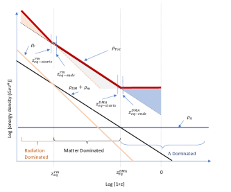
Figure 1: The evolution Radiation ($\rho_{r}$), Matter ($\rho_{M}$) and Dark energy density. Insert is the evolution of total energy density($\rho_{Tot}$) with redshift. Although $|z_{end}-z_{start}|$, is comparatively small, it is not negligible.

V.5 Cosmological Constant Dominated Epoch

The cosmological constant is appealing in modelling of the evolution of the Universe because it enables better agreement between theory and observation. Generically, the gravitational pull exerted by the matter in the universe slows the expansion imparted by the Big Bang. The expansion can be estimated measurements involving supernovae. These observations seem to indicate that the universe is expanding at an accelerated rate raising the prospects of that a strange form of energy that has an effect that is the opposite of the standard gravitational pull. The cosmological constant seems to satisfy properties of such a strange form of energy. Nevertheless, it is not been conclusively established that dark energy is the non-dynamical cosmological constant Sol ; Wein ; Sah ; Pad ; Cop ; Shu ; Bloch ; Mart . We mention, without delving into a discussion, something of issues related to the cosmological constant, dark energy and the expansion of the universe. They include the fine-tuning problem and the cosmic coincidence problem. For a dark energy ($DDE+\Lambda$) dominated universe, we have

$$\dot{\rho}_{Tot} = -\left(1+\frac{1}{3}\alpha-\xi+\delta\omega_{DDE}+\beta\omega_{DM}\right)\theta\rho_{Tot}.$$ (39)

but $\alpha<<\xi$ and $\omega_{DM}=0$ yielding an effective equation of state of the form:

$$\omega_{eff} = -\xi+\delta\omega_{DDE}.$$ (40)

The bound $\dot{\rho}_{Tot}=0$ is analogous to an effective equation of state of the form $-1\leq\omega_{eff}$. This implies

$$-\xi+\delta\omega_{DDE}=-1.$$ (41)

There are several ways to interpret equation (41), (1) we could follow that standard folklore and allow $\omega_{DDE}=-1,$ which leads to $\xi+\delta=1$ or simply that the sum of dark sector fractions makes the total mass-energy density of the universe as a scenario that is yet to be reached. (2) The second possibility is to express the equation in the form $\omega_{DDE}=(\xi-1)/\delta$ , $\delta\neq 0$, which is negative since $\xi$ and $\delta$ are positive fractions less than 1.
As pointed out in Linder , the time-varying model with $\dot{\omega}>0$ behaviour, at high redshift, that is different from the cosmological constant. If we interpret cosmological constant as some form of dark energy, it follows that there may be other forms of dark energy that, at early times, is very different from the cosmological constant model but which quickly becomes dynamically negligible for $z>1$. This characteristic suggests that dark energy with time-varying EOS may exist and could be found in the low-multipole region of the CMB power spectrum as pointed out in Caldwell .

VI Discussion and Conclusion

It is customary to express the evolution of energy densities against scale factor as is shown in the lower section of Fig.1. The different epochs are then separated by points of intersection of the curves representing the various energy densities. The salient implication is that one single type of energy density dominates while all others play negligible or no role in the evolution of the total energy density. In this brief analysis, we have considered the evolution of the total energy density given the relative importance of the various energy densities constituents. This allows for a range of possibilities behaviour given the relative importance of a comparative fraction of each contributor. It is important to emphasise that the standard section of Fig.(1) (i.e. the lower section) emerges as the limiting case. We need to keep in mind the following issues, (i) we have assumed that the mass-energy material content of the universe is of perfect fluid form, (ii) the universe is of the Friedmann type with $\kappa=0$, (iii) that the interacting dark sector has no noticeable effect on the evolution of the total mass-energy density. These assumptions can be relaxed, and the resulting system(s) of equations analysed to obtain corrections to the standard model. Needless to say that the various ranges obtained here allow for a wide variety of matter-forms, for example, domain-wall with $\omega=-2/3$Nem . The effective equations of state for the total energy density discussed above may alter how fields evolve in the mixture. For example, the evolution of cosmological magnetic fields Tim may couple electrically to radiation and gravitationally to matter. Neglecting how one component evolves will therefore lead to an over or under estimation of the field strength. Some of these assertions will be examined in future.

VII Acknowledgement

The author thanks the University of Cape Town’s NGP for financial support.

Appendix A In redshift

Appendix B Some mathematical relations and relevant calculations

Basic formulae and step by step elementary calculations: Without loss of generality we write $\rho_{Tot}$ simply as $\rho$. Writing the expansion variable, $\theta$ in terms of the scale scalar, $a(t)$, and it time derivative yields:

$$\frac{\dot{\rho}(t)}{\rho(t)} = -3f(t)\frac{\dot{a(t)}}{a(t)},$$ (42)

where we have inserted variable $t$ to remind us of functions of this variable. This can be expressed as derivative notation as follows

$$\frac{d\ln\rho(t)}{dt} = -3f(t)\frac{d\ln a(t)}{dt}.$$ (43)

Integration by parts yields,

$$\ln\rho = -3f\ln a+3\int{(\ln a)\dot{f}dt}$$ (44)

which can be expressed as

$$\rho = a^{-3f}e^{3\int{(\ln a)\dot{f}dt}}.$$ (46)

Equation (44) can also be expressed in terms redshift as follows

$$\ln\rho = 3f\ln(1+z)-3\int{(\ln(1+z))\dot{f}dt},$$ (47)

where $1+z=\frac{a_{0}}{a}$ with $a_{0}$ taken as having the value unit. This is a more useful form for our visualisation. Dividing this through by $\ln(1+z)$ yields

$$\frac{\ln\rho}{\ln(1+z)} = 3f-\frac{3}{\ln(1+z)}\int{(\ln(1+z))\dot{f}dt}.$$ (48)

This is equivalent to

$$\frac{\ln\rho}{\ln(1+z)} = \frac{3}{\ln(1+z)}\int{\frac{\dot{z}}{1+z}fdt},$$ (49)

where $\dot{z}<0$.

Appendix C Fractional density

From equation (22) and noting that $f=f(t)$, then

$$f(t) = \frac{4}{3}\alpha(t)+\beta(t)+\gamma(t)(1+\omega_{DM})+\delta(t)(1+\omega_{DDE}).$$ (50)

In this formulation the the individual EOS for the constituents is not changing with respect to time but the effective EOS will. In particular,

$$\dot{f} = \frac{4}{3}\dot{\alpha}+\dot{\beta}+\dot{\gamma}+\dot{\delta}=\frac{1}{3}\dot{\alpha}-\dot{\xi}=-\dot{\omega}_{eff}.$$ (51)

This is the point of divergent with previous work in this area of research.

References

- (1) B. Ryden, Introduction to Cosmology, (Cambridge University Press, 2016).
- (2) M. Zelik and S. Gregory, Introductory Astronomy Astrophysics, (Thompson Learning, Inc., 1998).
- (3) P.J.E. Peebles, Principles of Physical Cosmology, (Princeton University Press, Princeton, 1993).
- (4) S. Weinberg, Gravitation and Cosmology: Principles and Applications of the General Theory of Relativity, (John Wiley Sons, New York, 1972).
- (5) S. Tian, The Relation between Cosmological Redshift and Scale Factor for Photons, Astrophy. Journal, 846:90 (2017).
- (6) M. Kopp, S. Constantinos, T. B. Daniel and S. Ili, (2018), Dark Matter Equation of State through Cosmic History Phys. Rev. Lett. 120, 221102.
- (7) R. J. Nemiroff and B. Patla, Adventures in Friedmann Cosmology: An Educationally Detailed Expansion of the Cosmological Friedmann Equations, Am. J. Phys.76 : 265-276, 2008.
- (8) P.J.E. Peebles and B. Ratra, The Cosmological Constant and Dark Energy, Rev. Mod. Phys.75 :559-606 (2003).
- (9) R. Durrer, What do we really know about Dark Energy?, Phil. Trans. R. Soc. A 369, 1957, 5102-5114.
- (10) Riess, A G et al., 1998, Observational Evidence from Supernovae for an Accelerating Universe and a Cosmological Constant Astron. J. 116, 2011, 1009-1038 [arXiv:astro-ph/9805201].
- (11) G. Hinshaw et al., 2013, Nine-Year Wilkinson Microwave Anisotropy Probe (WMAP) Observations: Cosmological Parameter Results, Astrophys. J. Suppl. 208, 19.
- (12) N. Aghanim et al., Planck 2018 results. VI. Cosmological parameters, arXiv:1807.06209 [astro-ph.CO].
- (13) A. G. Riess et al., 2018, Milky Way Cepheid Standards for Measuring Cosmic Distances and Application to Gaia DR2: Implications for the Hubble Constant Astrophys. J. 861 no. 2, 126.
- (14) S. Birrer et al., 2019, H0LiCOW - IX. Cosmographic analysis of the doubly imaged quasar SDSS 1206+4332 and a new measurement of the Hubble constant, Mon. Not. Roy. Astron. Soc. 484 (2019) 4726.
- (15) L. Knox and M. Millea, The Hubble Hunter’s Guide, preprint arXiv:1908.03663 [astro-ph.CO].
- (16) F. N. Chamings et al, Understanding the suppression of structure formation from dark matter–dark energy momentum coupling, preprint arXiv:1912.09858.
- (17) J. W. Rohlf, Modern Physics from a to Z0, (Wiley, 1994).
- (18) J. Sola, 2014, Vacuum energy and cosmological evolution AIP Conf. Proc. 1606 19-37
- (19) S. Weinberg, 1989, The cosmological constant problem, Rev. Mod. Phys. 6 1
- (20) V. Sahni, A. Starobinsky, 2000, The case for a Positive Cosmological Lambda-term, Int. J. of Mod. Phys. A9 373
- (21) T. Padmanabhan, (2003) Phys. Rept. 380, 235.
- (22) E. J. Copeland, M. Sami, S. Tsujikawa, (2006), Int. J. Mod. Phys. D 15,1753.
- (23) T. Oreta and B. Osano, Post inflationary evolution of inflation-produced large-scale magnetic fields using a generalised cosmological Ohm’s law and both standard and modified Maxwell’s equations, preprint arXiv:1912.08712.
- (24) I. M. Bloch et al, (2020),Crunching Away the Cosmological Constant Problem: Dynamical Selection of a Small , JHEP12,191.
- (25) J. Martin, Everything You Always Wanted To Know About The Cosmological Constant Problem (But Were Afraid To Ask), C. R. Physique 13,(2012),566-665.
- (26) W. Press et all, Numerical Recipes: The art of scientific Computing ( Cambridge University Press, 2007).
- (27) S. Perlmutter et al, Measurements of and from 42 hight-redshift supernovae, Astrophys. J. (1999)517:565-586.
- (28) B. Famaey et al, Baryon-Interacting Dark Matter: heating dark matter and the emergence of galaxy scaling relations, JACP06 (2020) 025.
- (29) S. Vagnozzi, New physics in light of the tension: an alternative view Phys. Rev. D 102, 023518 (2020).
- (30) W. Yang et al, (2018), Tale of stable interacting dark energy, observational signatures, and the tension JCAP 1809, 019.
- (31) E. Di Valentino et al , (2020) Interacting dark energy in the early 2020s: a promising solution to the and cosmic shear tensions J Phys. Dark Univ. 30,100666.
- (32) E. V. Linder and A. Jenkins, Cosmic structure growth and dark energy, Mon. Not. R. Astron. Soc. 346, 573-583 (2003).
- (33) R. R. Caldwell et al, Early Quintessence in Light of the Wilkinson Microwave Anisotropy Probe, ApJ, 591, 2003, L75