sKPNSGA-II: Knee point based MOEA with self-adaptive angle for Mission Planning Problems

Abstract

Real-world and complex problems have usually many objective functions that have to be optimized all at once. Over the last decades, Multi-Objective Evolutionary Algorithms (MOEAs) are designed to solve this kind of problems. Nevertheless, some problems have many objectives which lead to a large number of non-dominated solutions obtained by the optimization algorithms. The large set of non-dominated solutions hinders the selection of the most appropriate solution by the decision maker. This paper presents a new algorithm that has been designed to obtain the most significant solutions from the Pareto Optimal Frontier (POF). This approach is based on the cone-domination applied to MOEA, which can find the knee point solutions. In order to obtain the best cone angle, we propose a hypervolume-distribution metric, which is used to self-adapt the angle during the evolving process. This new algorithm has been applied to the real world application in Unmanned Air Vehicle (UAV) Mission Planning Problem. The experimental results show a significant improvement of the algorithm performance in terms of hypervolume, number of solutions, and also the required number of generations to converge.

I Introduction

Real-world optimization problems often deal with multiple objectives that must be met simultaneously in the solutions. In most cases, objectives are conflicting, so improving one objective usually cannot be achieved unless other objective is worsened. Such problems are called Multi-Objective Optimization Problems (MOPs), the solution of which is a set of solutions representing different performance trade-off between the objectives.

Most of the existing algorithms focus on the approximation of the Pareto Optimal Frontier (POF) in terms of convergence and distribution, but always with a fixed population size, which in the end, for complex problems with many solutions, returns an amount of individuals equal or similar to this population. Nevertheless, when this approximation of the Pareto set comprises a large number of solutions, the process of decision making to select one appropriate solution becomes a difficult task for the Decision Maker (DM). Sometimes, the DM provides a priori information about his/her preferences, which can be used in the optimization process [1, 2]. However, very often this information is not provided by the DM, and it is necessary to consider other approaches to filter the number of solutions. In opposition to the common trend of returning a more or less fix amount of solutions, it should be taken into account the hardness of decision making for every additional solution, which in the end may not be optimal enough in comparison with other solutions. So, for complex real-world problems, it should be considered to provide a lower amount of solution maintaining as much as possible of the convergence and distribution of the POF.

In the last years, finding the ”knee points” [3] have been used in several algorithms [4, 5] to deal with large POFs in convex problems when the DM does not provide preferences about the MOP. In this work, a new Multi-Objective Evolutionary Algorithm (MOEA) focused on the search of Knee Points is presented. This new algorithm changes the concept of domination to cone-domination, where a larger portion (cone region) than a typical domination criteria is considered when the solution frontier is generated. In this paper, the main novelty with respect to a previous approach [6] lies in the proposition of a new adaptive technique to find the right angle for the cone-domination which focus on reducing as much as possible the number of solutions while maintaining as much as possible the convergence and distribution of the POF.

We apply our proposed algorithm to the real-world Mission Planning Problem in which a team of Unmanned Air Vehicles (UAVs) must perform several tasks in a geodesic scenario in a specific time while being controlled by several Ground Control Stations (GCSs). In this context, there are several variables that influence the selection of the most appropriate plan, such as the makespan of the mission, the cost or the risk. Some experiments have been designed for evaluating the decrement of the number of solutions obtained, while maintaining the most significant ones.

This paper has been organized as follows. Section II provides some basics on MOPs and an introduction to the main concepts of Cone Domination. Section III presents the novel Knee-Point based Evolutionary Multi-Objective Optimization approach. In Section IV-A this new algorithm is evaluated using a set of real Mission Planning Problems, and compared against our previous approach. Finally, Section V presents several conclusions that have been achieved from current work.

II Background

This section provides the background and related works concerning the cone-domination and metrics upon which is our proposed algorithm is based.

II-A Multi-Objective Optimization

In most MOPs, it is not possible to find one single optimal solution that could be selected as the best one; so in this kind of problems there is usually a set of solutions that represent several agreements between the given criteria. Any minimization MOP can be formally defined as:

$$min\,\mathbf{f}(\mathbf{x})=(f_{1}(\mathbf{x}),f_{2}(\mathbf{x}),...,f_{m}(\mathbf{x}))^{T}$$

$$\text{subject to }\mathbf{x}\in\Omega\subseteq\mathbb{R}^{n}$$ (1)

where $\mathbf{x}=(x_{1},x_{2},...,x_{n})^{T}$ represents a vector of $n$ decision variables, which are taken from the decision space $\Omega$; $\mathbf{f}:\Omega\rightarrow\Theta\subseteq\mathbb{R}^{m}$, where $f$ represents a set of $m$ objective functions, and it is possible to define a mapping from $n$-dimensional decision space $\Omega$ to $m$-dimensional objective space $\Theta$.

Definition 1

Given two decision vectors $\mathbf{x},\mathbf{y}\in\Omega$, $\mathbf{x}$ is said to Pareto dominate $\mathbf{y}$, denoted by $\mathbf{x}\prec\mathbf{y}$, iff:

$$\forall i\in\{1,2,...,m\}\quad f_{i}(\mathbf{x})\leq f_{i}(\mathbf{y})$$

$$\exists j\in\{1,2,...,m\}\quad f_{j}(\mathbf{x})<f_{j}(\mathbf{y})$$ (2)

Definition 2

A decision vector $\mathbf{x}^{*}\in\Omega$, is Pareto optimal if $\nexists\mathbf{x}\in\Omega$, $\mathbf{x}\prec\mathbf{x}^{*}$.

Definition 3

The Pareto set $PS$, is defined as:

$$PS=\{\mathbf{x}\in\Omega|\mathbf{x}\text{ is Pareto optimal}\}$$ (3)

Definition 4

The Pareto front $PF$, is defined as:

$$PF=\{\mathbf{f}(\mathbf{x})\in\mathbb{R}^{m}|\mathbf{x}\in PS\}$$ (4)

The goal of MOEA is to find the non-dominated objective vectors which are as close as possible to the $PF$ (convergence) and evenly spread along the $PF$ (diversity). Non-dominated Sorting Genetic Algorithm-II (NSGA-II) has been one of the most popular algorithms over the last decade in this field [7]. This algorithm generates a non-dominated ranking in order to look for the convergence, and crowding distance to assure the diversity of the solutions. Other popular algorithms are SPEA2 [8], MOEA/D [9] and NSGA-III [10]. These last two algorithms have become very popular in the last years for their good performance on Many-Objective Optimization Problems (MaOPs).

II-B Knee Points and Cone Domination

In the last decade, several MOEAs have been proposed to search for non-dominated solutions located close to a given reference point that incorporates the preference of the DM [11]. However, some a priori knowledge is require to set the reference point, which many times the DM does not have. With the aim of obtaining significant solutions when no a priori knowledge is provided, the concept of finding ”knee points” [12] can be used. In this way, we reduce the size of the non-dominated set and provide the DM a small set of so-called knee point solutions. When distinct knee points are present in the Pareto front, most DMs would prefer the solutions in these points, because if a near solution to a knee point (trying to improve slightly one objective) is selected, it will generate a large worsening at least in one of the other objectives. An example showing the difference between a knee point (blue) and points that are not knee points (red) is shown in Figure 1.

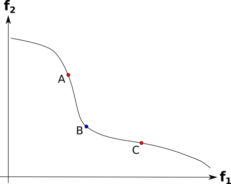
Figure 1: A synthetic simple example of a Pareto Front in a bi-objective minimization problem, where B is a knee point, while A and C, that have worse trade off than A, are not.

The concept of using knee points has been studied before. Branke et al. [3] presented a modification of NSGA-II where the crowding distance criterion is computed using angle-based and utility-based measures for focusing on knee points. In Schütze et al. [13] two different update methods are presented, these methods are based on maximal convex bulges that allow to focus the algorithm search on the knee points. Bechikh et al. [14] extended the reference point NSGA-II so the normal boundary intersection method is used to emphasize knee-like points. Zhang et al. [5] designed KnEA, an elitist Pareto-based algorithm that uses Knee point neighbouring as a secondary selection criteria in addition to dominance relationship.

In this paper, an angle-based measure is used to guide and focus the searching process on the knee points. Therefore, the concept of domination criterion has been changed to cone-domination. The cone-domination has been defined as a weighted function that manages the set of objectives [12]. This concept can be formally described as:

$$\Omega_{i}(\mathbf{f}(\mathbf{x}))=f_{i}(\mathbf{x})+\sum_{j=1,j\neq i}^{m}a_{ij}f_{j}(\mathbf{x}),\quad i=1,2,...,m$$ (5)

where $a_{ij}$ is the amount of gain in the $j$-th objective function for a loss of one unit in the $i$-th objective function. The matrix $\mathbf{a}$, composed of these $a_{ij}$ values, and with 1 values in its diagonal elements, has to be provided in order to apply the above equations.

Definition 5

A solution $\mathbf{x}$ is said to cone-dominate a solution $\mathbf{y}$, denoted by $\mathbf{x}\prec^{c}\mathbf{y}$, if:

$$\forall i\in\{1,2,...,m\}\quad\Omega_{i}(\mathbf{f}(\mathbf{x}))\leq\Omega_{i}(\mathbf{f}(\mathbf{y}))$$

$$\exists j\in\{1,2,...,m\}\quad\Omega_{j}(\mathbf{f}(\mathbf{x}))<\Omega_{j}(\mathbf{f}(\mathbf{y}))$$ (6)

In a bi-objective problem, the two ($m=2$) related objective weighted functions, can be defined as follows:

$$\Omega_{1}(f_{1},f_{2})=f_{1}+a_{12}f_{2}$$ (7)

$$\Omega_{2}(f_{1},f_{2})=a_{21}f_{1}+f_{2}$$ (8)

Previous equations can also be formalized as:

$$\mathbf{\Omega}=\begin{bmatrix}1&a_{12}\\[3.00003pt] a_{21}&1\end{bmatrix}\mathbf{f},\quad\text{or, }\mathbf{\Omega}=\mathbf{a}\mathbf{f}$$ (9)

In Figure 2(b) it is shown the contour lines for our previous two linear functions when these pass through a solution $P$ in objective space. The set of solutions inside those contour lines (the ”cone-dominated region”) will be dominated by $P$ according to the previous definition of domination. It is specially interesting to remark that when the standard definition of domination is used (see Figure 2(a)), the region between the horizontal and vertical lines will be dominated by $P$. Therefore, from both figures can be concluded that using the cone-domination definition will obtain larger regions (as the angle is greater than $90^{\circ}$), so more solutions will be dominated by one solution $P$ than when traditional definition is used. Therefore, and using the concept of cone-domination, the whole Pareto optimal front (using the traditional definition of domination), may not be non-dominated according to this new definition.

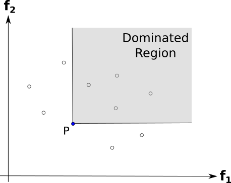
(a) Pareto Dominated Region.

(b) Cone Dominated Region.

Figure 2: Regions dominated by a solution P (2.a) using the original definition of domination in a 2-objectives problem, and cone-dominated (2.b) by the same solution when the concept of cone domination is used.

Besides, in Figure 2(b) it can be observed that the values $a_{12}$ and $a_{21}$ expand the $\varphi$ angle modifying the dominated region (whose value in the original definition of Pareto dominance is $90^{\circ}$). In this example, the vertical axis is rotated by the angle of $\varphi_{12}$, whereas the horizontal axis is rotated by $\varphi_{21}$. As it is shown in this figure, both angles are related to the $a_{12}$ and $a_{21}$ values, respectively, as follows:

$$tan\,\varphi_{12}=a_{12}$$ (10)

$$tan\,\varphi_{21}=a_{21}$$ (11)

Using previous equations, the new angle for the new dominated region of point $A$ will be $\varphi=90^{\circ}+\varphi_{12}+\varphi_{21}$. If the values of the objectives are normalized, to make the dominated region symmetric and thus equalize the turn of both horizontal and vertical axes (i.e. $\varphi_{12}=\varphi_{21}$), both variables of the matrix must also be equalized: $a_{12}=a_{21}=tan\frac{\varphi-90}{2}$. Then, the cone-domination considers angles, ($\varphi_{12},\varphi_{21}$) $\in$ [$90^{\circ}$, $180^{\circ}$], where the 90 degrees case is the common Pareto dominance, and the 180 degrees is equivalent to a weighted sum multi-objective optimization where all weights are the same (i.e. a single-objective optimization using the sum of all objectives as fitness function). In this last case, all the solutions are inside the same line of cone-domination, and the matrix $\mathbf{a}$ considered is filled with 1 ($\forall i,j\quad a_{ij}=1$).

In other cases, the cone domination concept can be formally defined as:

$$\mathbf{\Omega}=\begin{bmatrix}1&tan\frac{\varphi-90}{2}\\[3.00003pt] tan\frac{\varphi-90}{2}&1\end{bmatrix}\mathbf{f}$$ (12)

With the aim of comparing the convergence and diversity of the knee points obtained, in contrast with the Pareto front from the original approach, a study of several values of the angle $\varphi\in(90,180)$ must be carried out.

Now, let extend this concept to higher dimensions. For three dimension ($m=3$), in this case, having $\mathbf{f}=(f_{1},f_{2},f_{3})^{T}$, the cone domination function $\mathbf{\Omega}=\mathbf{a}\mathbf{f}$ is expressed as:

$$\mathbf{\Omega}=\begin{bmatrix}1&a_{12}&a_{13}\\[3.00003pt] a_{21}&1&a_{23}\\[3.00003pt] a_{31}&a_{32}&1\end{bmatrix}\mathbf{f}$$ (13)

Figure 3(a) shows the 3D contour corresponding to cone-dominated region for a solution $A$ in the objective space, where the bold lines converging in $A$ represent the edges of the cone region. In dashed lines, the edges used in the normal definition of Pareto domination for $A$ are also presented. As in the 2D case, the modified definition of domination allows a larger region to become dominated by any solution than the usual definition.

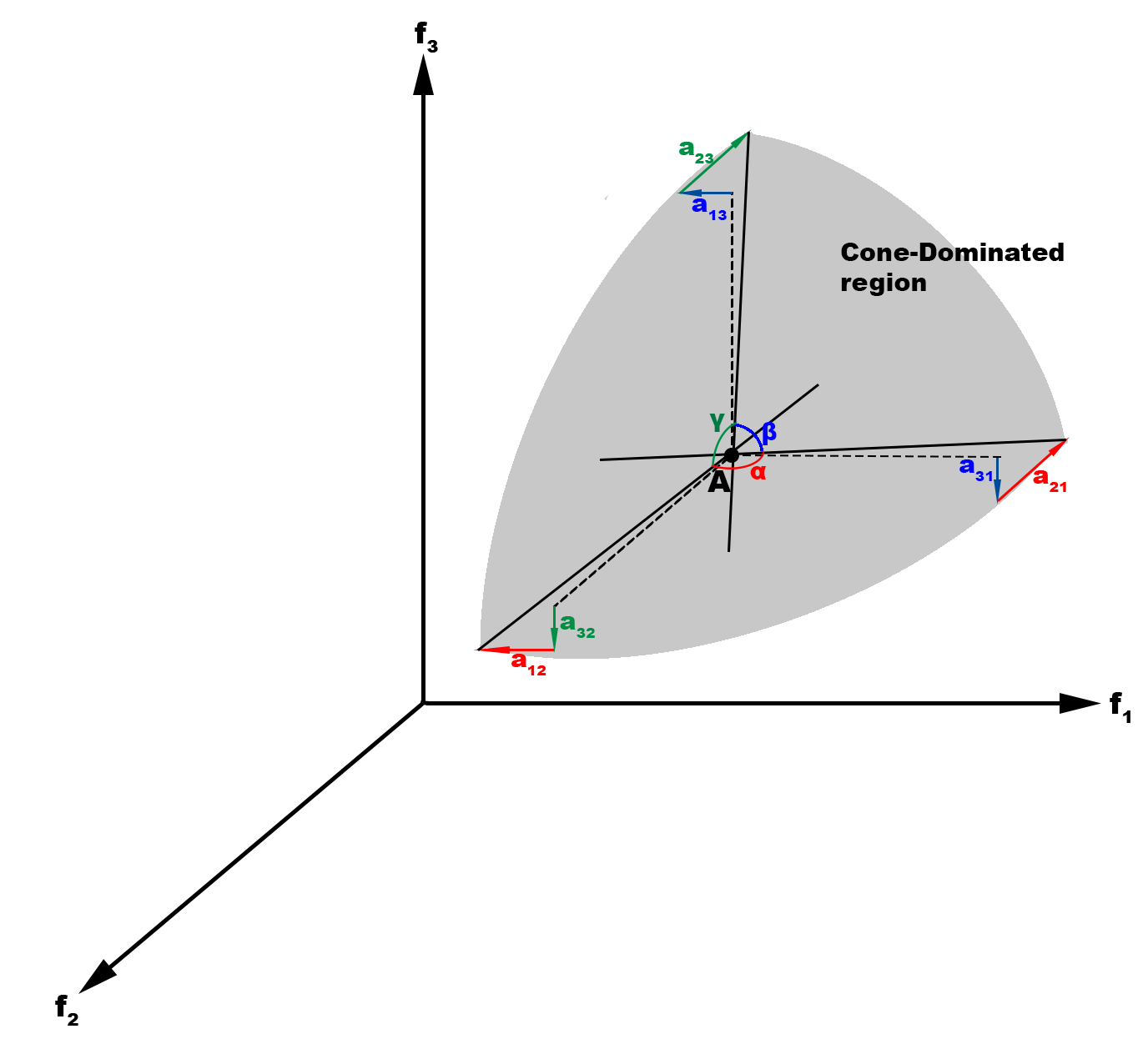
(a) Cone Dominated Region.

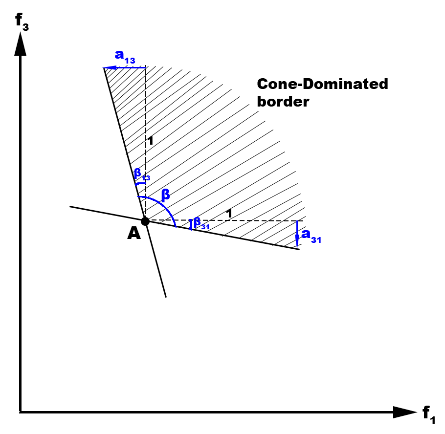
(b) Projection in the f1-f2 plane.

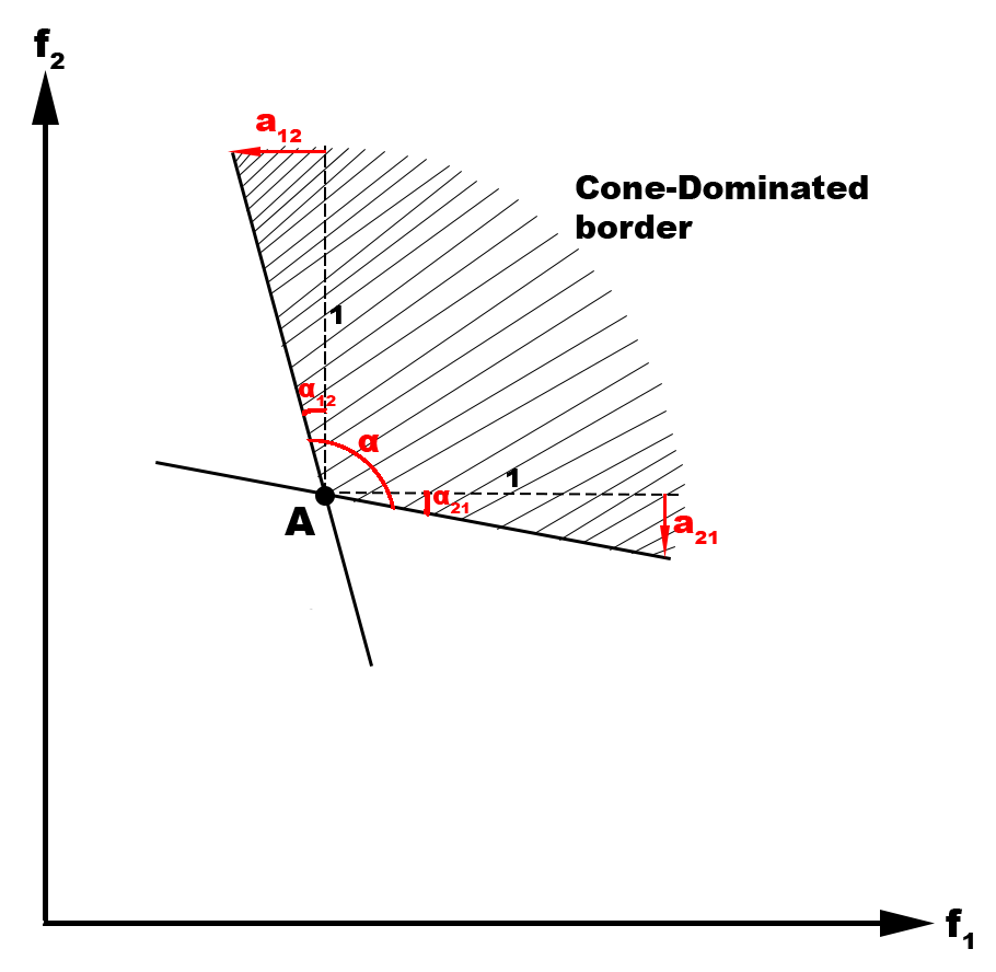
(c) Projection in the f1-f3 plane.

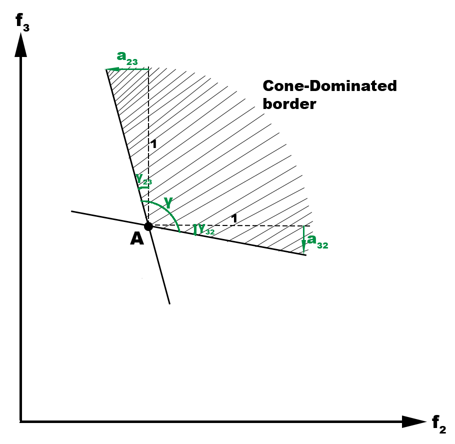
(d) Projection in the f2-f3 plane.

Figure 3: Regions cone-dominated by solution A in a 3-objective problem

Besides, Figures 3(b), 3(c) and 3(d) show the projections of this 3D region into the $f_{1}$-$f_{2}$ plane, $f_{1}$-$f_{3}$ plane and $f_{2}$-$f_{3}$ plane, respectively. These projections show a similarity with the cone-domination region for 2-objectives problems (see Figure 2(b)). In Figure 3(b) it is observable that the values $a_{12}$ and $a_{21}$ change the dominated region by expanding the $\alpha$ value, rotating the f1 axis an angle of $\alpha_{21}$ and the f2 axis an angle of $\alpha_{12}$. On the other hand, Figure 3(c) shows how values $a_{13}$ and $a_{31}$ expand the $\beta$ angle, rotating the f1 axis an angle of $\beta_{31}$ and the f3 axis an angle of $\beta_{13}$. Finally, Figure 3(d) shows how values $a_{23}$ and $a_{32}$ expand the $\gamma$ angle, rotating the f2 axis an angle of $\gamma_{32}$ and the f3 axis an angle of $\gamma_{23}$. As can be seen, similarly to the 2D cone-domination, the angles described and values of matrix $\mathbf{a}$ can be formulated as follows:

$$tan\,\alpha_{12}=a_{12},\quad tan\,\alpha_{21}=a_{21},$$

$$\alpha=90+\alpha_{12}+\alpha_{21}$$ (14)

$$tan\,\beta_{13}=a_{13},\quad tan\,\beta_{31}=a_{31},$$

$$\beta=90+\beta_{13}+\beta_{31}$$ (15)

$$tan\,\gamma_{23}=a_{23},\quad tan\,\gamma_{32}=a_{32},$$

$$\gamma=90+\gamma_{23}+\gamma_{32}$$ (16)

Following this reasoning, the cone-dominated region is defined by extending the angle of the region in 2-objective problems, while in 3-objective problems it is defined by extending the three angles of the faces defining the 3D cone. When considering a higher dimension $N$, a hypercone region with $\begin{pmatrix}N\\ 2\end{pmatrix}$ faces (and therefore, angles) is generated. This number is the result of the pair-combinations of the N objective functions. In this case, the cone domination is expressed as:

$$\mathbf{\Omega}=\begin{bmatrix}1&a_{12}&\dots&a_{1n}\\[3.00003pt] a_{21}&1&\dots&a_{2n}\\[3.00003pt] \vdots&\vdots&\ddots&\vdots\\[3.00003pt] a_{n1}&a_{n2}&\dots&1\end{bmatrix}\mathbf{f}$$ (17)

where each value $a_{ij}$ with $i\neq j,\;i,j\in\{1,2,...,N\}$ is related to the angle $\theta_{ij}$ so $tan\,\theta_{ij}=a_{ij}$. Besides, the angle $\theta^{ij}$ of the face $f_{i}$-$f_{j}$ of the hypercone region, is related to this angle (hence, $\theta^{ij}$ can be calculated as $\theta^{ij}=90+\theta_{ij}+\theta_{ji}$).

Again, and in order to make the cone dominated region symmetric for every objective, and supposing that the values of the objectives are normalized, it is necessary to equalize the angles of every face of the hypercone region. The definition of this angle $\theta$ leads to the setting of the values $a_{ij}$ of matrix $\mathbf{a}$:

$$a_{ij}=tan\frac{\theta-90}{2},\;\forall i,j\in\{1,2,...,N\},\;i\neq j$$ (18)

II-C Hypervolume and distribution of solutions

In order to evaluate the convergence and distribution of the non-dominated solutions obtained with MOEAs, some metrics have been proposed over the last decades [15]. One of the most popular is the Hypervolume (HV) [16], which gives the volume (in the objective space) that is dominated by some reference point. Other frequently used metric is the Inverted Generational Distance (IGD) [17], where a set of reference points is provided as an approximation of the Pareto front, and the IGD is computed as the distance from each reference point to the nearest solution in the solution set.

When the number of non-dominated solutions is large, the decision making process afterwards becomes really complex. In order to avoid this, the best outcome of the algorithm should be a small set of solutions maintaining as large as possible value for the HV or IGD. As the IGD is pretty complex to compute due to the need of a reference set, which in real problem is sometimes difficult to provide, the HV metric has been used to design a new metric that takes into account the number of solutions. We propose the hypervolume-distribution (HDist) metric, which is designed in order to evaluate this trade-off between HV and the number of solutions. This metric is defined as follows:

$$HDist(S,P)=\frac{\sharp(P)-\sharp(S)}{\sharp(P)}\times\frac{HV(S)}{HV(P)}$$ (19)

where $P$ is the POF of the problem, $S\subset P$ is the set of non-dominated solutions to be evaluated, and $HV:\mathbb{R}^{n}\rightarrow\mathbb{R}$ represents the hypervolume of the set. In this metric, the Pareto set is needed in order to normalize the number of solutions and the hypervolume, which are then combined. The higher the value of this metric, the better distributed solutions maintaining good hypervolume.

Using this metric, our main goal is to self-adapt the cone-domination angle in the evolving phase of the MOEA, so that the best set of non-dominated solutions according to the HDist metric is obtained.

III sKPNSGA-II: a self-adaptive Knee-point based extension of NSGA-II

In order to reduce the number of obtained solutions in a MOP, we propose an extension of NSGA-II, which is designed to search Knee-points instead of non-dominated solutions. To reach this goal, the cone-domination concept described in section II-B will be used instead of the standard Pareto-domination. The non-dominated ranking used by NSGA-II is changed to a non-cone-domination ranking with an specific angle $\theta$. In a previous work [6], a first approach called Knee-Point based NSGA-II (KPNSGA-II), using cone-domination with a fixed cone angle, was proposed. In this work, we propose self-adaptive Knee-Point based NSGA-II (sKPNSGA-II), which self-adapts the cone angle according to the $HDist$ metric proposed in previous section. In order to perform this self-adaptation, the golden section search [18] has been used. This technique is used to find the maximum value for the $HDist$ metric through a successive narrowing of the the range of values in which the maximum point is located.

The sKPNSGA-II is presented in Algorithm 1. This novel approach, after randomly generating the initial population (Line 1), initializes the convergence factors (Lines 2-4). Following this step, the maximum and minimum values for each objective is initialized to a zero-vector $q$ (line 5), and to the vector $\overline{M}$ of maximum objective values (Line 6), respectively. Every time the solutions are evaluated, these values are updated. Their aim is to be used in the normalization of the objective values.

Input: A problem $P$. The set of $m$-objectives $O$ and their upper bounds $\overline{M}=\{M_{i}>>avg(o_{i})\}$. And a set of positive parameters: $\mu$ (elitism), $\lambda$ (population size), $mutprobability$, $stopGen$ (stopping criteria limit), and $maxGen$ (maximum number of generations). $\phi=\frac{\sqrt{5}+1}{2}$ is the golden ratio.

Output: The Knee-Point Frontier generated

1 $S\leftarrow$ set of $\lambda$ individuals randomly generated

2 $i\leftarrow 1$

3 $convergence\leftarrow 0$

4 $kpof\leftarrow\emptyset$

5 $maxP\leftarrow[0,...,0]^{q}$

6 $minP\leftarrow\overline{M}$

7 $\theta,\theta_{A},\theta_{C}\leftarrow 90$

8 $\theta_{B},\theta_{D}\leftarrow 180$

9 while $i\leq maxGen\land convergence<stopGen$ do

10       for $j\leftarrow 1$ to $|S|$ do

11             $f.objectives\leftarrow MultiObjectiveFitness(S_{j},O)$

12             $maxP\leftarrow maxPerElem(maxP,f.objectives)$

13             $minP\leftarrow minPerElem(minP,f.objectives)$

14             $S_{j}.fit\leftarrow f$

15            

16      $S\leftarrow buildArchive(S,\lambda,\theta,maxP,minP)$

17       $newkpof\leftarrow kneeFront(S,\theta,maxP,minP)$

18       if $newkpof=pof$ then

19             $convergence\leftarrow convergence+1$

20            

21      $goldenSection(newkpof,\theta,\theta_{A},\theta_{B},\theta_{C},\theta_{D})$

22       $kpof\leftarrow newkpof$

23       $newS\leftarrow SelectElites(S,\mu)$

24       for $j\leftarrow\mu$ to $\lambda$ do

25             $p1,p2\leftarrow TournamentSelection(S$)

26             $i1,i2\leftarrow Crossover(p1,p2)$

27             $i1\leftarrow Mutation(i1,mutprobability)$

28             $i2\leftarrow Mutation(i2,mutprobability)$

29             $newS\leftarrow newS\cup\{i1,i2\}$

30            

31      $S\leftarrow S\cup newS$

32      

33return kpof

Algorithm 1 Self-adaptive Knee-Point based NSGA-II.

The fitness function (Lines 10-14) used in the evaluation of the individuals computes the multi-objective values of the solutions, which are stored inside the fitness. Moreover, as previously mentioned, the maximum and minimum objective values are updated with the new evaluated solutions (Lines 12-13).

Based on the NSGA-II algorithm, the new offspring is updated with the buildArchive function (Algorithm 1, line 15), which is presented in Algorithm 2. This function creates an array of vectors, or fronts, storing the solutions grouped by their level of non-cone-dominance. This is done using the assignFrontRanks function (see Algorithm 3). In this levelled array, the first front is composed of the non-cone-dominated solutions of the population; the second front contains the non-cone-dominated solutions among the rest of the population without considering the solutions of the first front; the third front is then composed of the non-cone-dominated solutions of the population without considering the solutions of the first and second fronts, and so on.

Input: Vector $S$ containing the actual population. Population size $\lambda$. Angle $\theta$ for every face of the cone. Vector $maxP$ stores the maximum values found for the $q$ objectives. Vector $minP$ stores the minimum values found for all $q$ objectives.

Output: Updated vector $S$

1 $newS\leftarrow\emptyset$

2 $ranks\leftarrow assignFrontRanks(S,\theta,maxP,minP)$

3 for $i\leftarrow 1$ to $|ranks|$ do

4       $rank\leftarrow ranks[i]$

5       $assignSparsity(rank,maxP,minP)$

6       if $|rank|+|newS|\geq\lambda$ then

7             $rank\leftarrow sort(rank)$

8             $newS\leftarrow newS\cup subVector(rank,0,\lambda-|newS|)$

9            

10      else

11             $newS\leftarrow newS\cup rank$

12            

13      

14return newS

Algorithm 2 BuildArchive($S,\lambda,\theta,maxP,minP$)

Input: Vector $S$ containing the actual population. Angle $\theta$ for every face of the cone. Vector $maxP$ stores the maximum values found for the $q$ objectives. Vector $minP$ stores the minimum values found for all $q$ objectives.

Output: List of vectors containing the solutions with same rank values.

1 $rankedFronts\leftarrow\emptyset$

2 $inds\leftarrow S$

3 $rank\leftarrow 1$

4 while $|inds|>0$ do

5       $front\leftarrow kneeFront(inds,\theta,maxP,minP)$

6       $inds\leftarrow inds-front$

7       for $j\leftarrow 1$ to $|front|$ do

8             $front[j].fitness.rank\leftarrow rank$

9            

10      $rankedFronts\leftarrow rankedFronts\cup\{front\}$

11       $rank\leftarrow rank+1$

12      

13return $rankedFronts$

Algorithm 3 assignFrontRanks($S,\theta,maxP,minP$)

In order to create the array of ranked fronts, the kneeFront function is used (see Algorithm 4). This function is similar to the classical one used in NSGA-II to generate the Pareto front from a population. Nevertheless, it has been changed, so instead of the non-dominated solutions, the function will consider the non-cone-dominated solutions, as was described in Section II-B. The new approach of cone domination is described in detail in Algorithm 5. Then, kneeFront function requires a $\theta$ value indicating the angle of the cone-domination. First, the objective vectors are normalized with the maximum and minimum values. Then, the cone-domination function is computed using the Equations 5 and 18 for each objective; and the function examines if the second solution is cone-dominated by the first.

Input: Vector $S$ containing the actual population. Angle $\theta$ for every face of the cone. Vector $maxP$ stores the maximum values found for the $q$ objectives. Vector $minP$ stores the minimum values found for all $q$ objectives.

Output: Knee-Point Frontier based on the Cone-Domination with angle $\theta$.

1 $front\leftarrow\{S[1]\}$

2 for $i\leftarrow 2$ to $|S|$ do

3       $noOneWasBetter\leftarrow TRUE$

4       for $j\leftarrow 1$ to $|front|$ do

5             if $ConeDom(S[j],S[i],\theta,maxP,minP)$ then

6                   $noOneWasBetter\leftarrow FALSE$

7                  

8            else if $ConeDom(S[i],S[j],\theta,maxP,minP)$ then

9                   $front\leftarrow front-S[j]$

10                   $j\leftarrow j-1$

11                  

12            

13      if $noOneWasBetter$ then

14             $front\leftarrow front\cup S[i]$

15            

16      

17return $front$

Algorithm 4 kneeFront($S,\theta,maxP,minP$)

Input: Solutions A and B, used to check for cone-domination. The angle $\theta$ (in degrees) for every face of the cone. Vectors $maxP$ and $minP$ store the maximum and minimum values found for all $m$ objectives.

Output: TRUE if A dominates B, FALSE otherwise.

1 $\mathbf{x}\leftarrow\frac{A.fit.objectives-minP}{maxP-minP}$

2 $\mathbf{y}\leftarrow\frac{B.fit.objectives-minP}{maxP-minP}$

3 $dominates\leftarrow$ FALSE

4 for $i\leftarrow 1$ to $m$ do

5       $cone1\leftarrow\mathbf{x}[i]$

6       $cone2\leftarrow\mathbf{y}[i]$

7       for $j\leftarrow 1$ to $m$ do

8             $cone1\leftarrow cone1+tan(\frac{\theta-90}{2})\cdot\mathbf{x}[j]$

9             $cone2\leftarrow cone2+tan(\frac{\theta-90}{2})\cdot\mathbf{y}[j]$

10            

11      if $cone1<cone2$ then

12             $dominates\leftarrow$ TRUE

13            

14      if $cone1>cone2$ then

15             return FALSE

16            

17      

18return $dominates$

Algorithm 5 ConeDom($A,B,\theta,maxP,minP$)

Once the array of vectors containing the ranked solutions is created, in a similar way to NSGA-II algorithm, a sparsity value (that is based on the crowding distance) is given to each solution at every vector, through the assignSparsity function in Algorithm 2.

In order to self-adapt the cone angle according to the $HDist$ metric, the Golden Section Search has been used (Line 19). This technique is used to find the maximum of the $HDist$ metric iteratively as the main algorithm evolves. It is described in Algorithm 6. This technique is similar to the bisection search for the root of an equation. Specifically, if in the neighbourhood of the maximum we can find three points $x_{A}<x_{C}<x_{B}$ corresponding to $f(x_{A})>f(x_{C})<f(x_{B})$, then there exists a maximum between the points $x_{A}$ and $x_{B}$. To search for this maximum, we can choose another point $x_{D}$ between $x_{C}$ and $x_{B}$ as shown in the figure 4. Then, depending on the value of $f(X_{D})$, the new triplet may become $x_{A}<x_{C}<x_{D}$ if $f(X_{D})=f_{D2}<f(X_{C})$, or $x_{C}<x_{D}<x_{B}$ if $f(X_{D})=f_{D1}>f(X_{C})$. And so, the process is repeated iteratively until an error tolerance is reached. In order to compute these points $x_{C}$ and $x_{D}$, the golden ratio $\phi$ is used, where each point is separated from the corner points $x_{A}$ and $x_{B}$ the distance between these corner points divided by $\phi$.

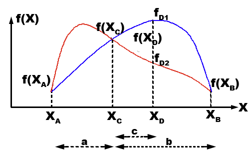
Figure 4: Diagram of the Golden Section Search.

In sKPNSGA-II, the golden section search starts working once the front has a large number of solutions or the hypervolume does not show a considerable increase with respect to previous generations. Then, the $\theta_{C}$ cone angle value is tested in the following generation, and then the $\theta_{D}$ in the next one. After testing both, they are compared as previously described, the triplet is updated and the process continues until the stopping criteria is met.

Input: Vector $S$ containing the actual knee front. Angle $\theta$ being used. Angles used in the golden section search $\theta_{A}$, $\theta_{B}$, $\theta_{C}$ and $\theta_{D}$.

1 $hyp\leftarrow HV(newkpof)$

2 $minHyp\leftarrow min(hyp,minHyp)$

3 $maxHyp\leftarrow max(hyp,maxHyp)$

4 $minPOF\leftarrow min(|newkpof|,minPOF)$

5 $maxPOF\leftarrow max(|newkpof|,maxPOF)$

6 if $\theta=90$ then

7       if $|newkpof|>\mu\quad\lor$ $HV(newkpof)-HV(kpof)<10^{-5}$ then

8             $\theta_{C}\leftarrow\theta_{B}-\frac{\theta_{B}-\theta_{A}}{\phi}$

9             $\theta_{D}\leftarrow\theta_{A}+\frac{\theta_{B}-\theta_{A}}{\phi}$

10             $\theta\leftarrow\theta_{C}$

11             $test_{C}\leftarrow true$

12            

13      

14else

15       if $test_{C}$ then

16             $HDist_{C}\leftarrow\frac{hyp-minHyp}{maxHyp-minHyp}\times\frac{maxPOF-|newkpof|}{maxPOF-minPOF}$

17             $\theta\leftarrow\theta_{D}$

18             $test_{C}\leftarrow false$

19            

20      else

21             $HDist_{D}\leftarrow\frac{hyp-minHyp}{maxHyp-minHyp}\times\frac{maxPOF-|newkpof|}{maxPOF-minPOF}$

22             if $HDist_{C}>HDist_{D}$ then

23                   $\theta_{B}\leftarrow\theta_{D}$

24                  

25            else

26                   $\theta_{A}\leftarrow\theta_{C}$

27                  

28            $\theta_{C}\leftarrow\theta_{B}-\frac{\theta_{B}-\theta_{A}}{\phi}$

29             $\theta_{D}\leftarrow\theta_{A}+\frac{\theta_{B}-\theta_{A}}{\phi}$

30             $\theta\leftarrow\theta_{C}$

31             $test_{C}\leftarrow true$

32            

33      

Algorithm 6 goldenSection($S,\theta,\theta_{A},\theta_{B},\theta_{C},\theta_{D}$)

Following Algorithm 1, a tournament selection (Line 23) is used to provide the individuals that will be chosen to apply the genetic operators. The crossover operator (line 24) and the mutation operator (lines 25-26) are then applied.

Finally, in this algorithm the stopping criteria considers the comparison of the non dominated solutions obtained so far at the end of each generation with the solutions from the previous generation (Lines 17-18). When the solutions obtained so far remain unchanged for a specific number of generations, the algorithm will stop and return the set of solutions found as the best approximation of the POF.

IV Experimental evaluation

In order to test the proposed algorithm, a real complex problem have to be considered where decision makers actually care about the number of solutions for the decision making process. In these experiments, several real Mission Planning Problems have been designed for this. Mission Planning[19] is a complex problem that involves the assignment of several tasks to the vehicles performing them, along with the assignments of vehicles to GCSs controlling them. Some tasks are performed by just one vehicle, while others may be performed by several vehicles reducing the time needed for the task (e.g. taking a photo, monitoring a target…). There exists several issues to take into account, such as the paths followed by the UAVs when there are No Flight Zones (NFZs) in the scenario, the sensors to be used by the vehicles for each task, the flight time or the fuel consumption, among others. In a previous work[20], this problem was modelled as a Constraint Satisfaction Problem (CSP), considering the different constraints of the problem (sensors, path, time, fuel…), and solved using a standard NSGA-II algorithm.

This problem is also a Multi-Objective Optimization problem, as there exist several objectives that influence the selection of the most appropriate plan. 7 objectives have been considered, that include: the total cost of the vehicles for completing the mission; the makespan or end time when all vehicles have returned and the mission is ended; or the risk of the mission, which has been calculated as an average percentage that indicates how hazardous the mission is (e.g. UAVs that end up with low fuel, UAVs that fly near to the ground or UAVs that fly close between them); the number of UAVs used in the mission, the total fuel consumption, the total flight time and the total distance traversed.

The fitness function used for this problem checks that all of the constraints considered are fulfilled for a given solution. If not, it stores inside its fitness the number of constraints fulfilled by the solution. When all constraints are fulfilled, the fitness will work as a multi-objective function minimizing the problem objectives.

The encoding considered here takes into account the different variables of the CSP model, which includes: the assignments of UAVs to tasks, the order of the tasks, the assignments of GCSs to UAVs, the flight profiles used in each path and return to the base, and the sensors used for each task performance. For this encoding, proper crossover and mutation operators have been designed, where a concrete operator is applied to each allele of the individuals. For more details about the encoding and the CSP model, may you consult previous works [19] [20].

In these experiments, we tested the newly implemented sKPNSGA-II with 12 different scenarios, represented in Figure 5). In these figures, the green zones represent tasks, while the red zones represent NFZs. There are also some point tasks represented with an icon, such as photographing, tracking or fire extinguishing. These scenarios are composed of an increasing number of tasks, multi-UAV tasks, UAVs, GCSs, NFZs and temporal dependencies between tasks (see Table I).

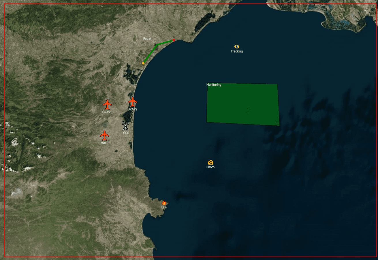
(a) Mission 1.

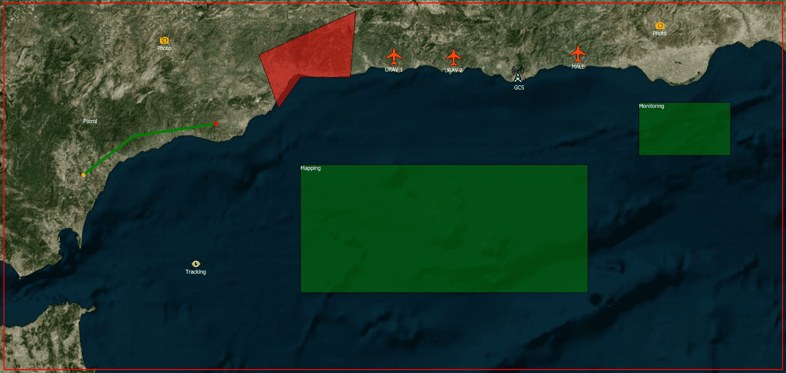
(b) Mission 2.

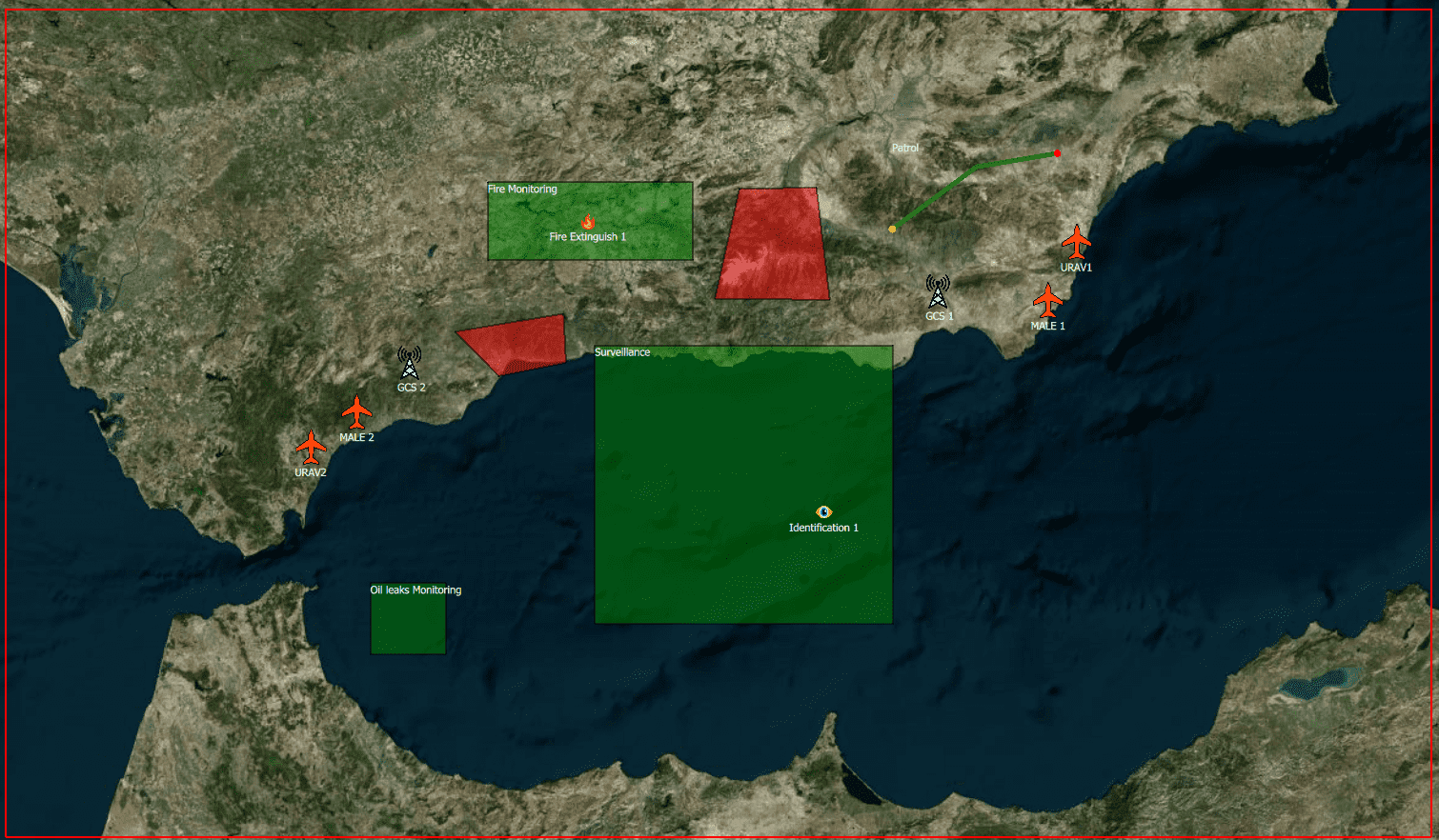
(c) Mission 3.

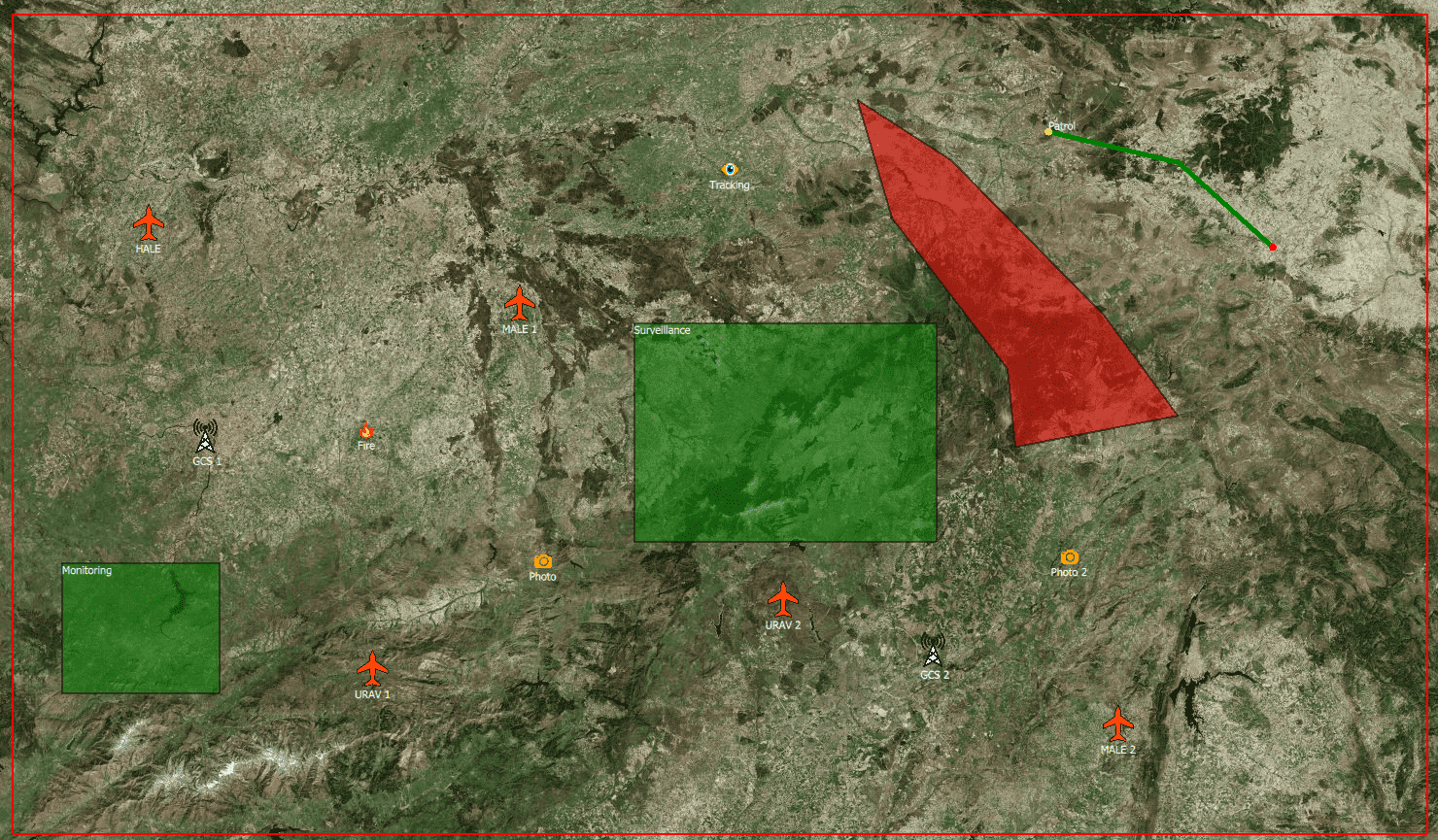
(d) Mission 4.

(e) Mission 5.

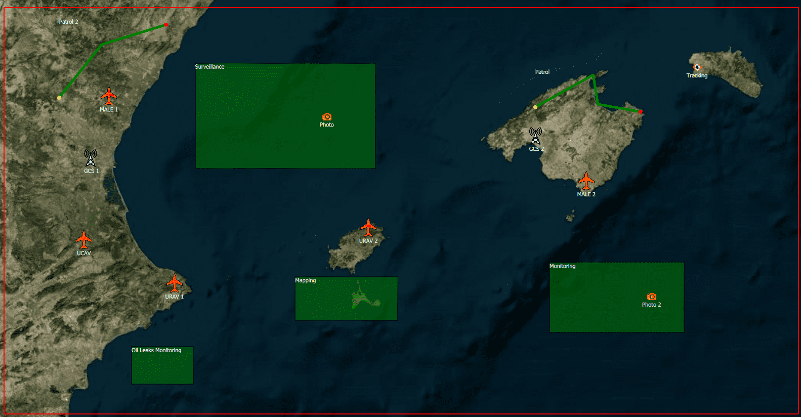
(f) Mission 6.

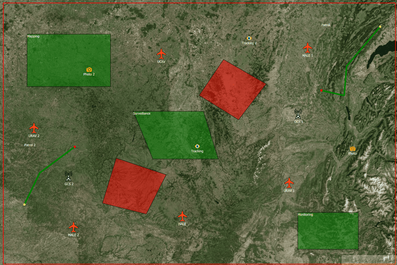
(g) Mission 7.

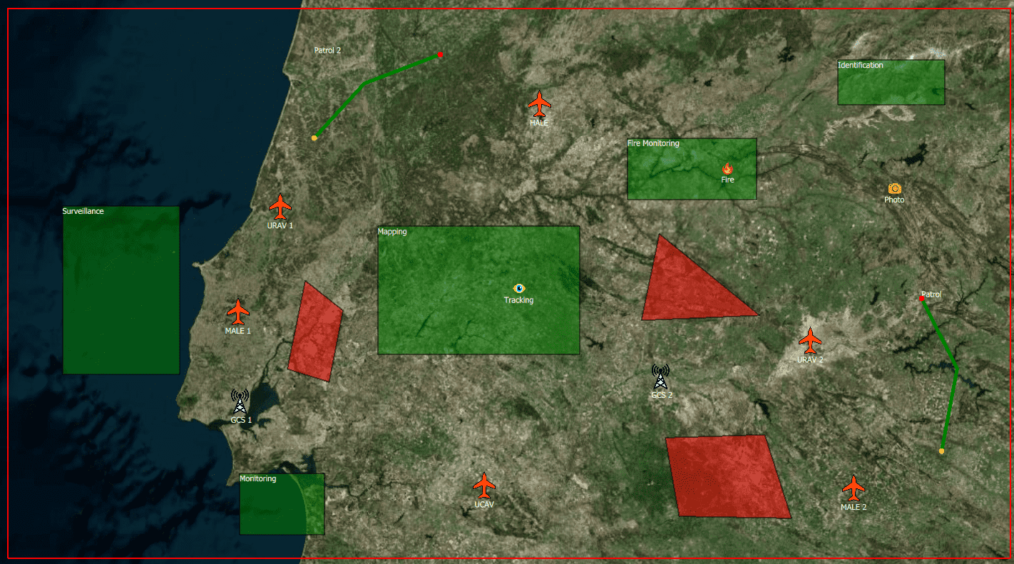
(h) Mission 8.

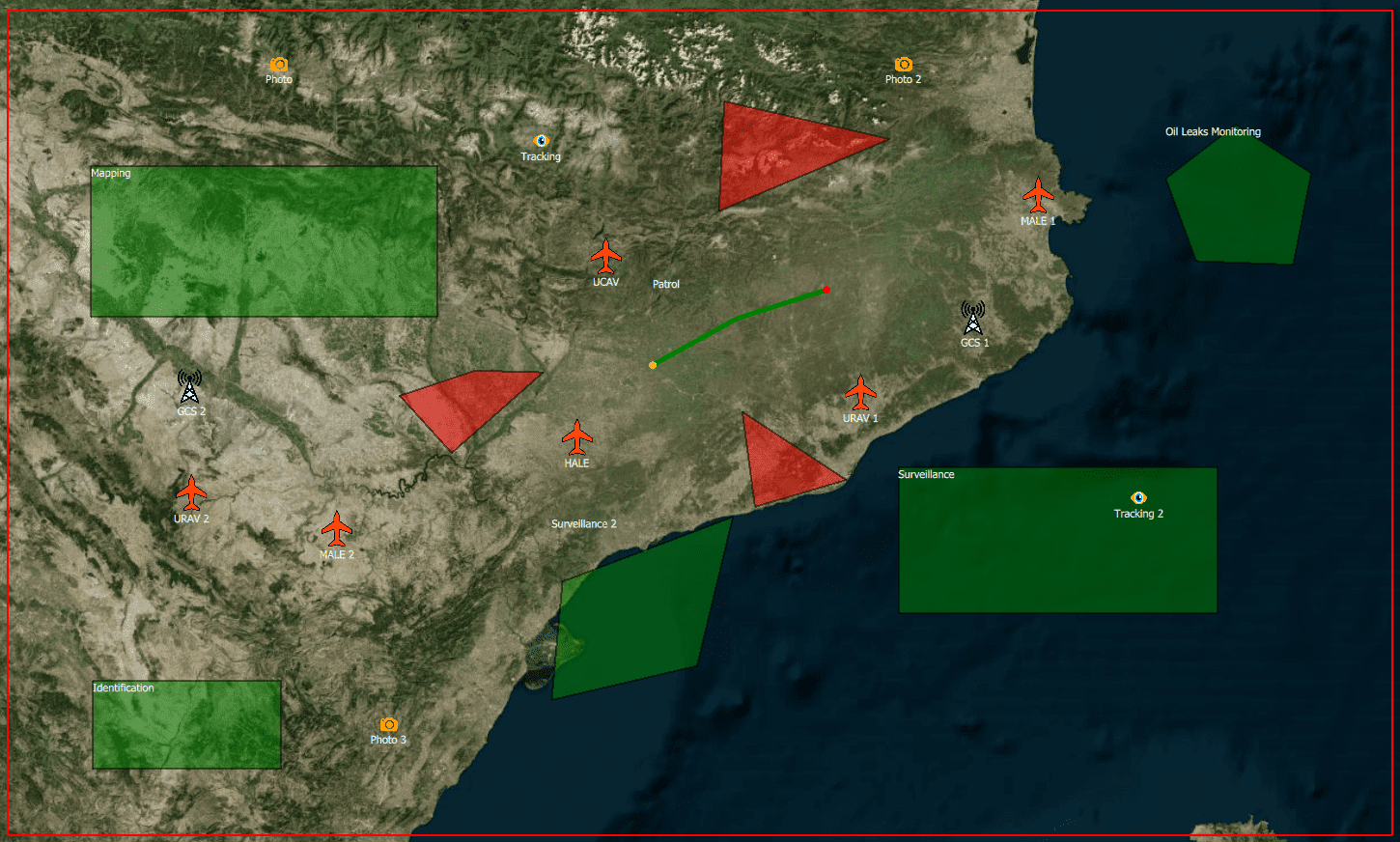
(i) Mission 9.

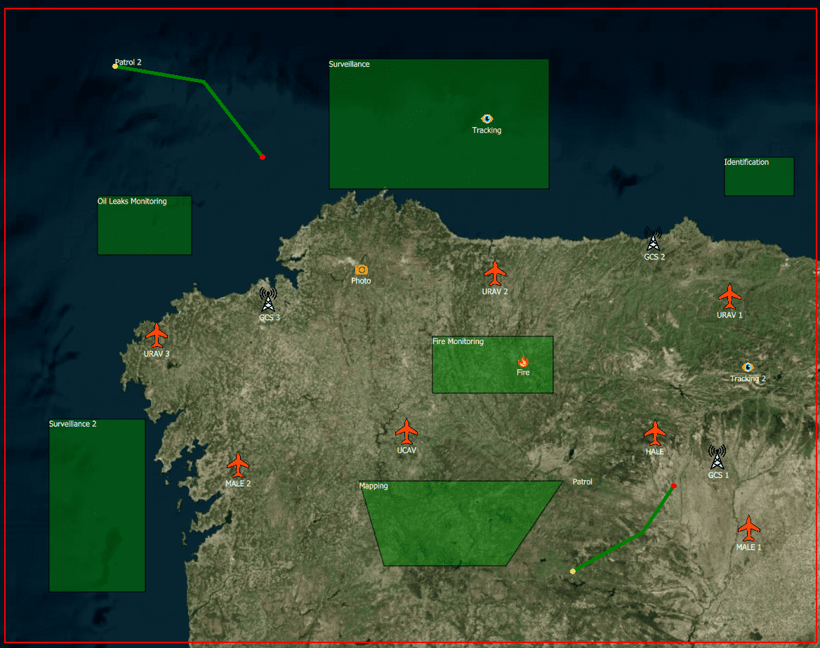
(j) Mission 10.

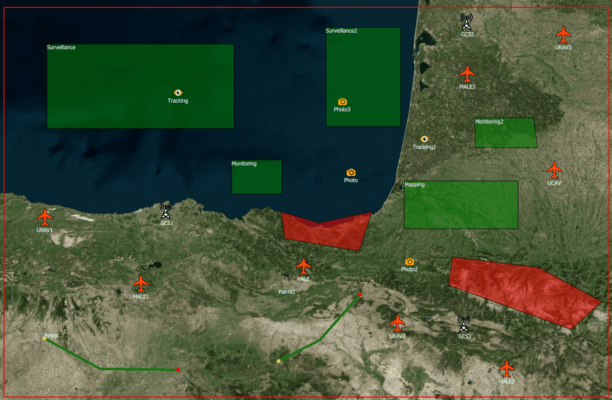
(k) Mission 11.

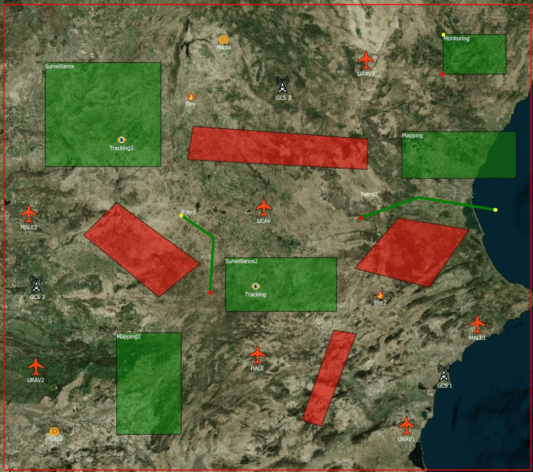
(l) Mission 12.

Figure 5: Mission Scenarios considered.

TABLE I: Main features (number of UAVs, GCs, NFZs, etc.) for the different missions designed.

Mission Id.	Tasks	Multi-UAV Tasks	UAVs	GCSs	NFZs	Time Dependencies
1	5	0	3	1	0	0
2	6	1	3	1	1	0
3	6	1	4	2	2	1
4	7	1	5	2	1	2
5	8	2	5	2	3	1
6	9	2	5	2	0	2
7	9	2	6	2	2	2
8	10	2	6	2	3	3
9	11	3	6	2	3	2
10	12	3	7	3	0	2
11	12	3	8	3	2	3
12	13	4	7	3	4	4

In the experiments, we tested these missions with the sKPNSGA-II algorithm developed in this work. In order to test the self-adaptation of the algorithm for the cone angle, the missions were also solved using NSGA-II and the cone-angle-dependant implementation KPNSGA-II [6] where the angle is fixed, using $120^{\circ}$, $135^{\circ}$, and $150^{\circ}$ angles (these approaches are names KPNSGA-II-120, KPNSGA-II-135 and KPNSGA-II-150, respectively).

Each experiment has been executed 30 times, and the mean and standard deviation are presented for all the tables. On the other hand, the rest of parameters have been set to: population of the algorithm to 200, maximum number of generations to 300, the mutation probability to $5\%$, and the stopping criteria to 10.

IV-A Experimental results

To compare the results obtained, we computed the hypervolume with the normalized objectives for each solution set, taking as reference point the maximum point $(1,1,1,...)$. These results are shown in Table II. On the other hand, Table III shows the number of solutions obtained for each approach.

TABLE II: Mean and standard deviation of the hypervolume obtained from the solutions given the different approaches for the different mission problems.

Id.	NSGA-II	KPNSGA-II-120	KPNSGA-II-135	KPNSGA-II-150	sKPNSGA-II
1	$0.826\pm 0.003$	$0.79\pm 0$	$0.783\pm 0.002$	$0.782\pm 0$	$0.785\pm 0.003$
2	$0.861\pm 0.002$	$0.72\pm 0.036$	$0.699\pm 0.019$	$0.693\pm 0$	$0.728\pm 0.045$
3	$0.892\pm 0.001$	$0.79\pm 0$	$0.78\pm 0.025$	$0.78\pm 0.025$	$0.793\pm 0.031$
4	$0.952\pm 0.003$	$0.889\pm 0.063$	$0.887\pm 0.031$	$0.886\pm 0.029$	$0.935\pm 0.02$
5	$0.839\pm 0.004$	$0.741\pm 0.062$	$0.636\pm 0.11$	$0.605\pm 0.091$	$0.688\pm 0.085$
6	$0.107\pm 0.008$	$0.095\pm 0.002$	$0.092\pm 0.004$	$0.088\pm 0.004$	$0.089\pm 0.006$
7	$0.227\pm 0.012$	$0.209\pm 0.006$	$0.203\pm 0.012$	$0.195\pm 0.018$	$0.201\pm 0.014$
8	$0.161\pm 0.015$	$0.14\pm 0.005$	$0.136\pm 0.004$	$0.132\pm 0.006$	$0.138\pm 0.004$
9	$0.122\pm 0.013$	$0.095\pm 0.008$	$0.091\pm 0.007$	$0.087\pm 0.007$	$0.091\pm 0.003$
10	$0.147\pm 0.017$	$0.123\pm 0.017$	$0.104\pm 0.015$	$0.107\pm 0.013$	$0.114\pm 0.017$
11	$0.161\pm 0.020$	$0.138\pm 0.011$	$0.124\pm 0.008$	$0.117\pm 0.01$	$0.134\pm 0.014$
12	$0.151\pm 0.022$	$0.132\pm 0.011$	$0.118\pm 0.016$	$0.11\pm 0.016$	$0.123\pm 0.008$

TABLE III: Mean and standard deviation of the number of solutions obtained from the different approaches for the different mission problems.

Id.	NSGA-II	KPNSGA-II-120	KPNSGA-II-135	KPNSGA-II-150	sKPNSGA-II
1	$89.32\pm 5.46$	$2\pm 0$	$1.05\pm 0.22$	$1\pm 0$	$1.3\pm 0.47$
2	$432.13\pm 10.51$	$1.44\pm 0.51$	$1.13\pm 0.35$	$1.06\pm 0.25$	$2.71\pm 2.52$
3	$517.53\pm 29.92$	$1\pm 0$	$1\pm 0$	$1\pm 0$	$1.36\pm 0.95$
4	$322.61\pm 42.7$	$2.7\pm 0.92$	$1.55\pm 0.51$	$1.5\pm 0.51$	$1.06\pm 0.24$
5	$342.24\pm 55.43$	$3.3\pm 1.56$	$1.9\pm 0.99$	$1.5\pm 0.83$	$2.65\pm 1.66$
6	$792.21\pm 83.12$	$4.04\pm 0.81$	$2.24\pm 0.72$	$1.6\pm 0.76$	$2.43\pm 2.92$
7	$1191.25\pm 116.74$	$4.08\pm 1.79$	$2.84\pm 1.21$	$2.08\pm 0.76$	$3.67\pm 3.94$
8	$692.98\pm 78.85$	$3.88\pm 3.89$	$1.8\pm 1.19$	$1.24\pm 0.52$	$2.07\pm 1.27$
9	$822.94\pm 115.24$	$7.58\pm 3.6$	$3.72\pm 2.82$	$1.8\pm 1.16$	$4.75\pm 1.5$
10	$579.25\pm 98.83$	$11.75\pm 7.71$	$3.84\pm 3.04$	$3.12\pm 1.81$	$4.5\pm 4.95$
11	$967.65\pm 126.79$	$17.83\pm 13.66$	$8.4\pm 5.8$	$3.8\pm 1.56$	$8.75\pm 9.07$
12	$484.52\pm 76.6$	$6.33\pm 3.84$	$3.52\pm 2.45$	$1.84\pm 1.21$	$1.36\pm 0.5$

In these results, it is appreciable how the hypervolume decreases with bigger angles, as well as the number of solutions. On the other hand, it is appreciable how NSGA-II gets worse results as the complexity of the problem grows (the difference of hypervolume with respect to sKPNSGA-II decreases), due to the big number of solutions composing the POF.

In order to measure these hypervolume and number of solutions together, the HDist metric (see Section II-C) is used. The values of this metric for each result are presented in Table IV. With this, we can clearly appreciate that sKPNSGA-II gets the best results for this metric, as it has been optimized during the evolutionary process. In addition, we have computed the Wilcoxon test [21], comparing sKPNSGA-II with the rest of approaches. The test succeed in all problems, with a $p-value<0.05$.

TABLE IV: Mean and standard deviation of the HDist metric obtained from the solutions of the different approaches for the different mission problems.

Id.	NSGA-II	KPNSGA-II-120	KPNSGA-II-135	KPNSGA-II-150	sKPNSGA-II
1	$0.046\pm 0.059$	$0.631\pm 0$	$0.587\pm 0.01$	$0.585\pm 0$	$0.599\pm 0.022$
2	$0.02\pm 0.024$	$0.16\pm 0.213$	$0.035\pm 0.113$	$0\pm 0$	$0.207\pm 0.261$
3	$0.095\pm 0.052$	$0.397\pm 0$	$0.337\pm 0.145$	$0.337\pm 0.145$	$0.413\pm 0.181$
4	$0.201\pm 0.103$	$0.777\pm 0.205$	$0.773\pm 0.098$	$0.771\pm 0.094$	$0.93\pm 0.065$
5	$0.194\pm 0.126$	$0.702\pm 0.161$	$0.428\pm 0.288$	$0.346\pm 0.241$	$0.564\pm 0.223$
6	$0.102\pm 0.098$	$0.801\pm 0.035$	$0.737\pm 0.067$	$0.678\pm 0.076$	$0.692\pm 0.095$
7	$0.088\pm 0.106$	$0.807\pm 0.064$	$0.735\pm 0.135$	$0.653\pm 0.197$	$0.711\pm 0.156$
8	$0.064\pm 0.056$	$0.534\pm 0.115$	$0.447\pm 0.092$	$0.355\pm 0.137$	$0.492\pm 0.085$
9	$0.078\pm 0.043$	$0.387\pm 0.146$	$0.299\pm 0.134$	$0.233\pm 0.135$	$0.31\pm 0.053$
10	$0.054\pm 0.026$	$0.701\pm 0.183$	$0.499\pm 0.17$	$0.535\pm 0.156$	$0.607\pm 0.198$
11	$0.021\pm 0.013$	$0.714\pm 0.131$	$0.552\pm 0.101$	$0.469\pm 0.118$	$0.668\pm 0.17$
12	$0.009\pm 0.012$	$0.818\pm 0.1$	$0.692\pm 0.15$	$0.617\pm 0.144$	$0.736\pm 0.069$

The results also show that the HDist metric presents a bigger standard deviation in sKPNSGA-II than in the rest of approaches. This can be better seen in the HDist graphic in Figure 6. This is specially appreciable in the most complex problems, and it is due to the early start of the golden section search algorithm due to the condition of the high number of solutions (see Algorithm 6, Line 7). Erasing this condition, will outperform the convergence of the approach, but at the expense of increasing the number of generations needed to converge and, consequently, the runtime of the algorithm.

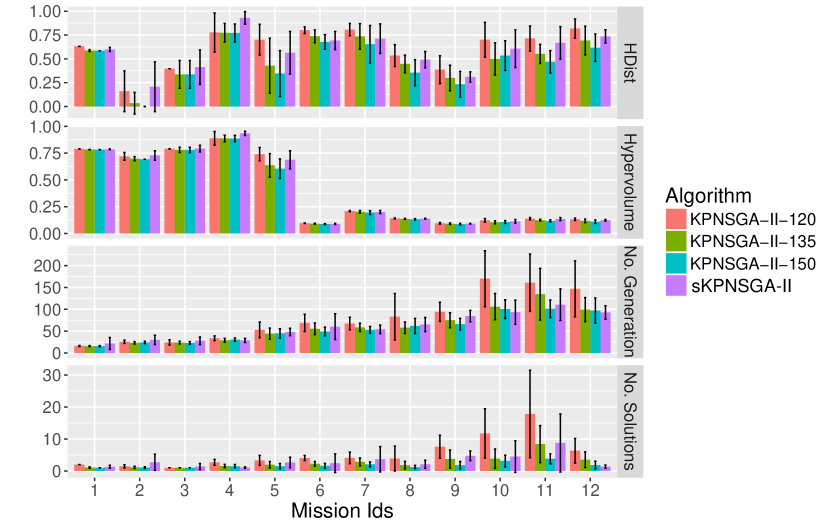
Figure 6: Comparison of hypervolume, number of solutions obtained, HDist metric and number of generations needed to converge for the different approaches in each problem.

Table V shows the number of generations needed to converge for the different missions and algorithms. Here, it is shown that the runtime of the algorithm is also reduced with sKPNSGA-II compared to NSGA-II, which in most cases was not even able to converge in the maximum number of generations defined. On the other hand, the runtime of sKPNSGA-II is bigger than the approaches where the angle is fixed. Concretely, the higher the cone angle, the faster the algorithm.

TABLE V: Mean and standard deviation of the number of generations needed to converge in the different approaches for the different mission problems.

Id.	NSGA-II	KPNSGA-II-120	KPNSGA-II-135	KPNSGA-II-150	sKPNSGA-II
1	$64.789\pm 14.273$	$16.048\pm 1.244$	$15.762\pm 1.091$	$15.571\pm 1.207$	$21.75\pm 13.78$
2	$271.875\pm 49.295$	$25.688\pm 3.737$	$23.267\pm 2.712$	$24.188\pm 2.664$	$29.941\pm 10.802$
3	$298.124\pm 2.54$	$24.25\pm 6.008$	$23.9\pm 2.936$	$23\pm 2.974$	$27.909\pm 8.717$
4	$300\pm 0$	$33.75\pm 5.466$	$29.15\pm 4.38$	$30.6\pm 3.47$	$28.722\pm 4.812$
5	$300\pm 0$	$53\pm 18.061$	$44.1\pm 12.732$	$44.8\pm 10.665$	$48.176\pm 8.465$
6	$300\pm 0$	$68.917\pm 19.64$	$55.4\pm 13.292$	$49.12\pm 10.035$	$60.286\pm 29.508$
7	$300\pm 0$	$67.5\pm 14.347$	$58.6\pm 9.341$	$52.84\pm 7.867$	$54.111\pm 9.752$
8	$300\pm 0$	$83.125\pm 53.161$	$57.84\pm 13.243$	$61.88\pm 17.302$	$65.071\pm 16.074$
9	$300\pm 0$	$94.167\pm 21.908$	$74.96\pm 17.155$	$66\pm 13.279$	$84.5\pm 13.077$
10	$300\pm 0$	$169.958\pm 63.995$	$106.12\pm 29.914$	$100.44\pm 21.389$	$93.5\pm 27.577$
11	$300\pm 0$	$160.792\pm 65.543$	$134.48\pm 59.178$	$101.2\pm 20.114$	$110.5\pm 36.189$
12	$300\pm 0$	$146.917\pm 63.827$	$99.32\pm 27.436$	$97.12\pm 28.642$	$92.714\pm 15.339$

In order to observe how sKPNSGA-II evolves, Figure 7 shows the evolution of Cone Angle, Hypervolume, Number of solutions obtained and HDist Metric by generation in Mission 4, and compares them with the fix angle approaches. Here, it is appreciable how the cone angle critically varies when the golden section search starts but rapidly converge to the optimum value. In the HDist graphic, it is shown how sKPNSGA-II starts with worse HDist than the other approaches as it has not determined its cone angle yet, but once it does, it get the better result.

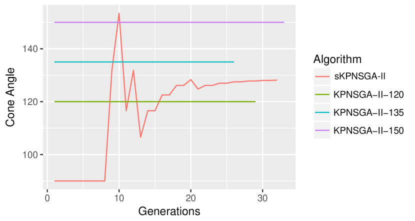
(a) Cone angle.

(b) Hypervolume.

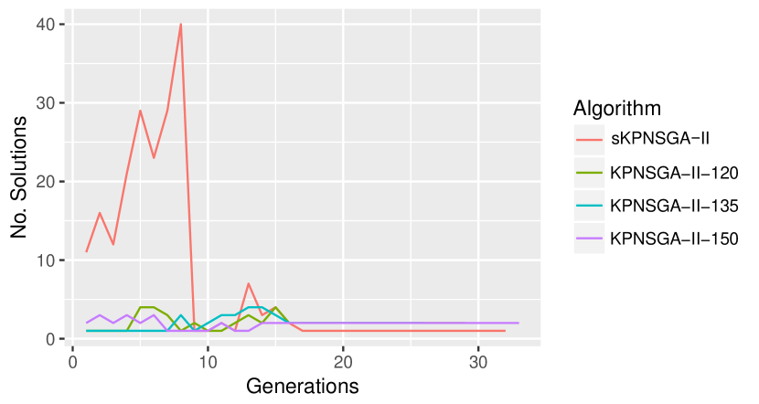
(c) Number of solutions.

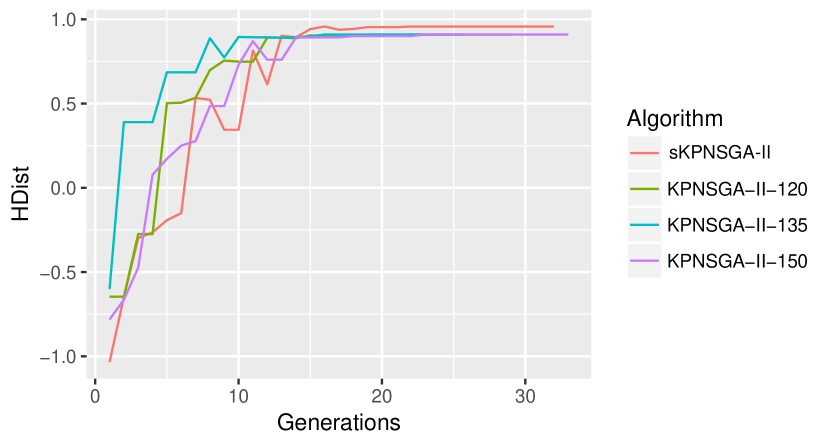
(d) HDist metric.

Figure 7: Evolution of metrics by generation for mission 4.

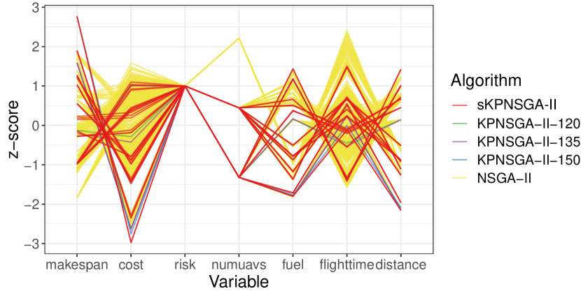
(a) Parallel plot.

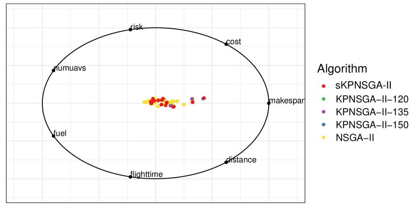
(b) Radial plot.

Figure 8: Visualization of solutions for mission 4.

On the other hand, Figure 8 shows the parallel and radial plot of the solutions obtained by each approach. Here, it can be seen how the solutions obtained by sKPNSGA-II are spread with all the optimization variables, proving that the solutions obtained are a significant sample of the solutions of the POF.

V Conclusion

In this work, we have presented an extension of the NSGA-II algorithm based on Knee Points in order to guide and focus the search process of the algorithm for significant solutions. To do that, we have presented the concept of cone-domination, which substitutes the domination concept in the algorithm. The algorithm uses a cone angle which self-adapts in the algorithm using the golden section search.

This new approach have been tested with real Multi-UAV Mission Planning Problems, which are complex and have a lot of solutions. In these problems, the mission operator has to select the best solution among all the obtained, so reducing the number of solutions and present just the most significant ones to the operator will reduce its workload.

In the experimental phase, the approach has been compared against NSGA-II and non-self-adapting approaches with three different cone angles (120, 135 and 150). The results showed that the sKPNSGA-II approach adapts the angle according to the HDist metric, which is clearly maximized when compared to the other approaches. The number of solutions returned are quite small while the most of the hypervolume is maintained compared to NSGA-II.

On the other hand, the results obtained from the experimental phase showed that the number of generations needed to converge are also improved by the new algorithm compared to NSGA-II, while the fixed angle approaches converge earlier. In the most complex problems, NSGA-II could not find the complete POF, while sKPNSGA-II could converge.

In our future research works, and in order to improve the decision making process for the operator, we will also develop some ranker algorithm for the solutions returned by sKPNSGA-II, which allows to easily select the most interesting and relevant solutions to human operators.

References

- [1] L. Thiele, K. Miettinen, P. J. Korhonen, and J. Molina, “A Preference-Based Evolutionary Algorithm for Multi-Objective Optimization,” Evolutionary Computation, vol. 17, no. 3, pp. 411–436, 2009.
- [2] F. Goulart and F. Campelo, “Preference-guided evolutionary algorithms for many-objective optimization,” Information Sciences, vol. 329, pp. 236–255, 2016.
- [3] J. Branke, K. Deb, H. Dierolf, and M. Osswald, “Finding knees in multi-objective optimization,” in Parallel Problem Solving from Nature - PPSN VIII. PPSN 2004. Lecture Notes in Computer Science, X. Yao, Ed., vol. 3242. Springer, Berlin, Heidelberg, 2004, pp. 722–731.
- [4] Y. Setoguchi, K. Narukawa, and H. Ishibuchi, “A Knee-Based EMO Algorithm with an Efficient Method to Update Mobile Reference Points,” in Evolutionary Multi-Criterion Optimization. EMO 2015. Lecture Notes in Computer Science, A. Gaspar-Cunha, C. Henggeler Antunes, and C. Coello Coello, Eds., vol. 9018. Springer, Cham, 2015, pp. 202–217.
- [5] X. Zhang, Y. Tian, and Y. Jin, “A knee point-driven evolutionary algorithm for many-objective optimization,” IEEE Transactions on Evolutionary Computation, vol. 19, no. 6, pp. 761–776, 2015.
- [6] C. Ramirez-Atencia, S. Mostaghim, and D. Camacho, “A Knee Point based Evolutionary Multi-objective Optimization for Mission Planning Problems,” in Genetic and Evolutionary Computation Conference (GECCO 2017). ACM, 2017, pp. 1216–1223.
- [7] K. Deb, A. Pratap, S. Agarwal, and T. Meyarivan, “A fast and elitist multiobjective genetic algorithm: NSGA-II,” Evolutionary Computation, vol. 6, no. 2, pp. 182–197, 2002.
- [8] E. Zitzler, M. Laumanns, and L. Thiele, “SPEA2: Improving the Strength Pareto Evolutionary Algorithm,” in Evolutionary Methods for Design Optimization and Control with Applications to Industrial Problems (EUROGEN 2001), K. C. Giannakoglou, D.T.Tsahalis, J.Periaux, and T. Fogarty, Eds. International Center for Numerical Methods in Engineering (CIMNE), 2002, pp. 95–100.
- [9] Q. Zhang and H. Li, “MOEA/D: A Multiobjective Evolutionary Algorithm Based on Decomposition,” IEEE Transactions on Evolutionary Computation, vol. 11, no. 6, pp. 712–731, 2007.
- [10] H. Jain and K. Deb, “An Improved Adaptive Approach for Elitist Nondominated Sorting Genetic Algorithm for Many-Objective Optimization,” in Evolutionary Multi-Criterion Optimization. EMO 2013. Lecture Notes in Computer Science, vol. 7811. Springer, Berlin, Heidelberg, 2013, pp. 307–321.
- [11] R. C. Purshouse, K. Deb, M. M. Mansor, S. Mostaghim, and R. Wang, “A review of hybrid evolutionary multiple criteria decision making methods,” in 2014 IEEE congress on evolutionary computation (CEC). IEEE, 2014, pp. 1147–1154.
- [12] K. Deb, P. Zope, and A. Jain, “Distributed computing of pareto-optimal solutions with evolutionary algorithms,” in International Conference on Evolutionary Multi-Criterion Optimization, vol. 2632. Springer, 2003, pp. 534–549.
- [13] O. Schütze, M. Laumanns, and C. A. Coello Coello, “Approximating the knee of an MOP with stochastic search algorithms,” in Parallel Problem Solving from Nature – PPSN X. PPSN 2008. Lecture Notes in Computer Science, G. Rudolph, T. Jansen, N. Beume, S. Lucas, and C. Poloni, Eds., vol. 5199. Springer Berlin Heidelberg, 2008, pp. 795–804.
- [14] S. Bechikh, L. B. Said, and K. Ghédira, “Searching for knee regions of the Pareto front using mobile reference points,” Soft Computing, vol. 15, no. 9, pp. 1807–1823, 2011.
- [15] S. Jiang, Y. S. Ong, J. Zhang, and L. Feng, “Consistencies and contradictions of performance metrics in multiobjective optimization,” IEEE Transactions on Cybernetics, vol. 44, no. 12, pp. 2391–2404, 2014.
- [16] C. Fonseca, L. Paquete, and M. Lopez-Ibanez, “An Improved Dimension-Sweep Algorithm for the Hypervolume Indicator,” in 2006 IEEE International Conference on Evolutionary Computation. IEEE, 2006, pp. 1157–1163.
- [17] H. Ishibuchi, H. Masuda, Y. Tanigaki, and Y. Nojima, “Difficulties in specifying reference points to calculate the inverted generational distance for many-objective optimization problems,” in IEEE SSCI 2014 - 2014 IEEE Symposium Series on Computational Intelligence - MCDM 2014: 2014 IEEE Symposium on Computational Intelligence in Multi-Criteria Decision-Making. IEEE, 2015, pp. 170–177.
- [18] W. H. Press, S. A. Teukolsky, W. T. Vetterling, and B. P. Flannery, Golden Section Search in One Dimension, 3rd ed. Cambridge University Press, 2007, no. 535, ch. 10.2, pp. 492–496.
- [19] C. Ramirez-Atencia and D. Camacho, “Constrained multi-objective optimization for multi-UAV planning,” Journal of Ambient Intelligence and Humanized Computing, vol. 10, no. 6, pp. 2467–2484, 2019.
- [20] C. Ramirez-Atencia, J. Del Ser, and D. Camacho, “Weighted strategies to guide a multi-objective evolutionary algorithm for multi-UAV mission planning,” Swarm and Evolutionary Computation, vol. 44, pp. 480–495, 2018.
- [21] M. Hollander, D. A. Wolfe, and E. Chicken, Nonparametric statistical methods, 3rd ed. John Wiley & Sons, Inc., 2014.