High order ADER schemes and GLM curl cleaning for a first order hyperbolic formulation of compressible flow with surface tension

Abstract

In this work, we introduce two novel reformulations of the weakly hyperbolic model for two-phase flow with surface tension, recently forwarded by Schmidmayer et al. In the model, the tracking of phase boundaries is achieved by using a vector interface field, rather than a scalar tracer, so that the surface-force stress tensor can be expressed directly as an algebraic function of the state variables, without requiring the computation of gradients of the scalar tracer. An interesting and important feature of the model is that this interface field obeys a curl involution constraint, that is, the vector field is required to be curl-free at all times.

The proposed modifications are intended to restore the strong hyperbolicity of the model, and are closely related to divergence-preserving numerical approaches developed in the field of numerical magnetohydrodynamics (MHD). The first strategy is based on the theory of Symmetric Hyperbolic and Thermodynamically Compatible (SHTC) systems forwarded by Godunov in the 60s and 70s and yields a modified system of governing equations which includes some symmetrisation terms, in analogy to the approach adopted later by Powell et al  in the 90s for the ideal MHD equations. The second technique is an extension of the hyperbolic Generalized Lagrangian Multiplier (GLM) divergence cleaning approach, forwarded by Munz et al  in applications to the Maxwell and MHD equations.

We solve the resulting nonconservative hyperbolic PDE systems with high order ADER Discontinuous Galerkin (DG) methods with a posteriori Finite Volume subcell limiting and carry out a set of numerical tests concerning flows dominated by surface tension as well as shock-driven flows. We also provide a new exact solution to the equations, show convergence of the schemes for orders of accuracy up to ten in space and time, and investigate the role of hyperbolicity and of curl constraints in the long-term stability of the computations.

a4paper, left=22.75mm, right=22.75mm, top=30mm, bottom=41.5mm spacing=nonfrench

1 Introduction

The necessity to develop mathematical models and numerical methods for explicit treatment of liquid-gas or liquid-liquid interfaces and accounting for the surface tension is well recognized in computational fluid mechanics. In particular, it is required in many applications relying on numerical simulations such as atomization [152], boiling and cavitation [95], additive manufacturing [91, 63], multi-phase flows in porous media [129] and microfluidics [160].

A great number of models and numerical methods have been proposed, and reviewing the vast literature existing on the topic is outside the scope of this paper. Instead, we refer the reader to some recent review articles in the field, e.g. [139, 124]. Each model and method has its own pros and cons, and usually the choice is conditioned by many factors. In particular, our preference is to develop a first-order hyperbolic model for surface tension which is motivated by our intention to further develop the unified first-order hyperbolic formulation for continuum mechanics forwarded in [120, 55, 56, 119]. Hyperbolic PDE systems have several attractive features for the numerical treatment. Namely, (i) the initial value problem for such systems is locally well posed; (ii) a quite general theory of hyperbolic PDEs can be established, e.g. [15, 33], and hyperbolic systems are subject to a unified numerical treatment (one may use one and the same numerical solver for various hyperbolic models representing totally different physics). In particular, this suggests a possibility for the development of a general purpose code [48]; (iii) first-order hyperbolic systems are less sensitive to the quality of the computational grid [113], have less restrictive stability conditions on the time-step [55], and in principle, the same nominal order of accuracy is achievable for all quantities, including those representing gradients in the high-order PDE models. In the last decade, models and computational approaches relying on hyperbolic equations have been developed for viscous Newtonian [120, 53, 112] and non-Newtonian [87] flows, for non-linear elastic and elastoplastic solids [72, 118, 54], for heat conduction [55, 119], for resistive electrodynamics [56], for dispersive equations [135, 103, 37], and for the Einstein field equations of gravity [49, 47].

Concerning the treatment of the material interfaces, one may in general distinguish the following computational approaches [139]. In Lagrangian schemes for compressible multi-material flows [16, 21, 93, 92] the interface is fully resolved and has thickness equal to zero. These algorithms are therefore also called sharp interface methods. In these approaches, the computational grid is aligned with the interface and deforms following the interface kinematics. These methods can be very accurate if the deformation of the interface is not too large, but they might be limited by mesh distortion at large deformations. Topological changes (break up, coalescences) are very difficult to implement in the Lagrangian framework, but they are at least in principle possible, see e.g. [145, 66]. Particle-based methods such as Smoothed Particle Hydrodynamics (SPH), see [70], can be also attributed to this class of methods and, while they solve the issues of mesh tangling by removing it completely, they lack the sharp description of material interfaces that characterise mesh-based Lagrangian methods and are more alike diffuse interface schemes in this regards. Furthermore, many SPH schemes also lack even zeroth order consistency and require artificial viscosity for stabilization, see [70, 105, 106], although this issue can be resolved using Riemann solver based SPH schemes [158, 62].

A different alternative strategy to model the interface dynamics consists in employing a method based on an Eulerian description of the governing equations, in order to avoid difficulties related to the mesh handling. In this class of methods, the interfaces are tracked implicitly via a new state variable that is often called colour function. Examples include the Level Set method (LSM) [115, 61, 148, 143] and the Volume of Fluid (VoF) approach [84, 140]. Eulerian methods are characterised by the fact that the interface (or rather, its implicit representation via a scalar tracer) is actually distributed (diffused) onto several grid cells. However, LSM and VoF are computational techniques that allow a subsequent reconstruction of a localised representation of the material boundaries (that is, with segments, polynomials, or other curves) and do not deal with the thermodynamics of the mixing zone (interface). Due to their explicit interface reconstruction, also level-set and VoF methods are considered sharp interface methods, although the interface is not explicitly resolved by the computational mesh, as in Lagrangian schemes.

Diffuse interface methods (DIM), instead, do not use any explicit interface reconstruction technique, but they are capable, by specifying directly at the PDE level the governing principles for mixed states, to represent complex non-equilibrium thermodynamics of the interface in many physical settings, e.g. phase transition and cavitation, mass transport, heat conduction, fluid-structure interaction, see e.g. [2, 137, 90, 117, 121, 60, 139, 67, 77, 78].

A fourth class of methods is that of Arbitrary Lagrangian Eulerian (ALE) schemes, see [43, 18, 19, 66] and references therein, which combine the Lagrangian mesh motion with an implicit representation of material discontinuities. This type of methods are particularly attractive as the mesh motion significantly reduces the smearing of contact discontinuities and of the scalar tracer variables that are employed for the description of material boundaries.

Purpose of the paper

The schemes employed in this work fall into the class of Eulerian methods and the proposed mathematical models follow a diffuse interface approach. In particular, the interface capturing between different phases is achieved by introducing a new vector interface field $\bm{\mathrm{b}}$, which represents the gradient of a colour function. This new vectorial quantity, i.e. the gradient of the colour function, is then explicitly evolved in time as a new independent state variable of the system, rather than performing a reconstruction of the phase boundaries from the colour function. In other works dealing with surface tension effects, the geometrical information on the direction of normal vectors and curvature of the interface is commonly obtained via post-processing of the scalar colour function, see [20, 114, 162, 147, 123, 125, 64].

In a sense, this methodology takes the diffuse interface approach further in the direction of decoupling the task of tracking material interfaces from a specific solution algorithm or code, in that we not only account for separation between different materials by means of a colour function to then recover geometrical information via a reconstruction technique, but we directly include the concept of an interface, a diffuse one specifically, at the PDE level. This significantly simplifies the use of general purpose high order methods to solve the resulting governing equations, as it allows writing the governing equations as a system of first order PDEs and eliminates the need for interface reconstruction procedures or finite-difference-type approximations in the computation of local curvature values and interface normal vectors. On the other hand, the downside of any first-order reduction of a high-order PDE system is the presence of so-called involution constraints in the former [80, 49, 47], which in general are stationary differential equations that are satisfied by the governing PDE system for all times if they are satisfied by the initial data. In particular in this paper we shall deal with the curl-type involution constraint on the vector field $\bm{\mathrm{b}}$

$$\nabla\times\bm{\mathrm{b}}=\bm{\mathrm{0}}.$$

Thus, from the numerical viewpoint, one may emphasise that the physical consistency of the numerical solution might be completely lost if the involution constraint is violated. The development of involution-constraint-preserving numerical methods is one of the key aspects in dealing with first-order reductions of high-order PDE systems.

The motivation for this paper is thus two-fold. First, we propose two separate ways of recovering a strongly hyperbolic formulation from the original weakly hyperbolic model for surface tension in compressible two-phase flow advanced by Gavrilyuk et al  in [17] and further developed by Schmidmayer et al  [141] . Both reformulations strongly rely on the curl-free constraint of the interface vector field $\bm{\mathrm{b}}$. Therefore, our second motivation for this paper was to systematically test the ability of the family of high-order ADER Discontinuous Galerkin (ADER-DG) [42, 45, 59, 164] and ADER Finite Volume (ADER-FV) schemes [150, 154, 151, 52, 46] designed for general systems of first order balance laws to deal with hyperbolic PDE systems with curl involution constraints, and to compare stability, accuracy and physical consistency of the proposed hyperbolic approaches with the original weakly hyperbolic formulation.

The first of the two reformulations of the model of Schmidmayer et al  [141] is based on the theory of Symmetric Hyperbolic and Thermodynamically Compatible (SHTC) systems [71, 76, 119], and consists in modifying the momentum and energy equations by adding some symmetrising nonconservative terms which are linear combinations of the involution constraint and thus, are formally zero at the continuum level. The approach is analogous to that used by Powell et al  in [126, 127] for the equations of ideal Magnetohydrodynamics and based on the ideas of Godunov [74], thus in this work we will refer to these non-conservative symmetrising terms as Godunov–Powell-type nonconservative products.

The second modified model is again based on ideas developed in the context of numerical Magnetohydrodynamics and specifically on the hyperbolic Generalized Lagrangian Multiplier (GLM) divergence-cleaning approach of Munz et al  [108, 34]. Thus, analogously to the GLM formulation for ideal MHD equations, which include an involution constraint on the divergence of the magnetic field, the surface tension model in consideration is augmented by a similar evolution equation for the additional curl-cleaning vector field. Such a GLM extension of the original model of Schmidmayer et al  [141] also allows to fix the issue with its weak hyperbolicity and makes the augmented GLM system again strongly hyperbolic.

The paper is organised as follows. In Section 2, we recall the features of the weakly hyperbolic Schmidmayer et al  [141] model and discuss the two modifications of the system which allow to recover strong hyperbolicity. We then provide an exact solution for cylindrically and spherically symmetric objects subject to surface tension forces, that would mean droplets and water jets, with some considerations on the implications on the diffuse interface treatment of such objects. We also explicitly compute the eigenvalues and a full set of eigenvectors for both of the new models proposed in this paper. In Section 3, we provide the details of the high-order ADER-DG and ADER-FV methods employed in this paper. Section 4 presents a set of test problems allowing to validate the new mathematical models and the numerical schemes proposed in this paper. Finally, the summary of the results as well as a discussion of further perspectives is given in Section 5.

2 Mathematical model

The original weakly hyperbolic two-phase, single velocity, single pressure model proposed in the paper of Schmidmayer et al  [141] can be written as follows:

$$\partial_{t}\left(\alpha_{1}\,\rho_{1}\right)+\nabla\cdot\left(\alpha_{1}\,\rho_{1}\,\bm{\mathrm{u}}\right)=0,$$ (1a)

$$\partial_{t}\left(\alpha_{2}\,\rho_{2}\right)+\nabla\cdot\left(\alpha_{2}\,\rho_{2}\,\bm{\mathrm{u}}\right)=0,$$ (1b)

$$\partial_{t}\left(\rho\,\bm{\mathrm{u}}\right)+\nabla\cdot\left(\rho\,\bm{\mathrm{u}}\otimes\bm{\mathrm{u}}+p\,\bm{\mathrm{I}}+\bm{\mathrm{\Omega}}\right)=\bm{\mathrm{0}},$$ (1c)

$$\partial_{t}\left(\rho\,E\right)+\nabla\cdot\left[\left(\rho\,E+p\right)\,\bm{\mathrm{u}}+\bm{\mathrm{\Omega}}\,\bm{\mathrm{u}}\right]=0,$$ (1d)

$$\partial_{t}\left(\alpha_{1}\right)+\bm{\mathrm{u}}\cdot\nabla\alpha_{1}-K\,\nabla\cdot\bm{\mathrm{u}}=0,$$ (1e)

$$\partial_{t}\left(\bm{\mathrm{b}}\right)+\left(\nabla\bm{\mathrm{b}}\right)\,\bm{\mathrm{u}}+{(\nabla\bm{\mathrm{u}})}^{\mathsf{T}}\,\bm{\mathrm{b}}=\bm{\mathrm{0}},\qquad\nabla\times\bm{\mathrm{b}}=\bm{\mathrm{0}},$$ (1f)

$$\partial_{t}\left(c\right)+\bm{\mathrm{u}}\cdot\nabla c=0.$$ (1g)

The model consists of two mass conservation equations (1a) and (1b), one for each of the two phases, a single (vector) equation (1c) for the conservation of mixture momentum $\rho\,\bm{\mathrm{u}}$ and one scalar equation (1d) for the conservation of the total energy of the mixture ${\rho\,E=\rho\,e+\tfrac{1}{2}\,\rho\lVert\bm{\mathrm{u}}\rVert^{2}+\sigma\,\lVert\bm{\mathrm{b}}\rVert}$, which includes a surface energy contribution $\sigma\,\lVert\bm{\mathrm{b}}\rVert$ to be added to the usual internal and kinetic energy terms. We denote ${\bm{\mathrm{u}}={\left(u,\ v,\ w\right)}^{\mathsf{T}}}$ and ${\bm{\mathrm{b}}={\left(b_{1},\ b_{2},\ b_{3}\right)}^{\mathsf{T}}}$, the former being the velocity field, the latter the interface field defined in the following paragraphs.

The nonconservative equation (1e) can be derived from the pressure equilibrium equation and the hypotheses about isentropic behaviour of each phase. Because the volume fractions $\alpha_{1}$ and $\alpha_{2}$ are subject to the constraint $\alpha_{1}+\alpha_{2}=1$, one equation is sufficient for the description of both. The mixture density is defined as $\rho=\rho_{1}\,\alpha_{1}+\rho_{2}\,\alpha_{2}$, where $\rho_{1}$ and $\rho_{2}$ are the densities of the first and the second phase, respectively. Neglecting surface tension effects, the first five equations of (1) are known as Kapila’s [90] five equation model, which is the stiff relaxation limit of the seven-equation Baer–Nunziato model [4]. The system is closed if the specific energy $e$ is given as a function of the other variables. In this work, we employ the so-called stiffened gas equation of state, in order to establish a biunivocal relation between the pressure of each phase $p_{1}$ or $p_{2}$ and the corresponding internal energy density $\rho_{1}\,e_{1}$ or $\rho_{2}\,e_{2}$ as follows:

$$p_{1}=\left(\gamma_{1}-1\right)\,\rho_{1}\,e_{1}-\gamma_{1}\,\Pi_{1},\qquad p_{2}=\left(\gamma_{2}-1\right)\,\rho_{2}\,e_{2}-\gamma_{2}\,\Pi_{2},$$ (2)

with $\gamma_{1}$, $\gamma_{2}$, $\Pi_{1}$, $\Pi_{2}$ given parameters of the equation of state. Due to the pressure equilibrium assumption $p_{1}=p_{2}=p$, the mixture equation of state then reads

$$p=\frac{\rho\,e\,\left(\gamma_{1}-1\right)\left(\gamma_{2}-1\right)-\alpha_{1}\,\gamma_{1}\,\Pi_{1}\,\left(\gamma_{2}-1\right)-\alpha_{2}\,\gamma_{2}\,\Pi_{2}\,\left(\gamma_{1}-1\right)}{\alpha_{1}\,\left(\gamma_{2}-1\right)+\alpha_{2}\,\left(\gamma_{1}-1\right)}.$$ (3)

Furthermore, for this choice of closure relation, we have

$$K=\frac{\alpha_{1}\,\alpha_{2}\,\left(\rho_{2}\,a_{2}^{2}-\rho_{1}\,a_{1}^{2}\right)}{\alpha_{1}\,\rho_{2}\,a_{2}^{2}+\alpha_{2}\,\rho_{1}\,a_{1}^{2}},\qquad\textnormal{with}\qquad a_{1}=\sqrt{\frac{\gamma_{1}\,\left(p+\Pi_{1}\right)}{\rho_{1}}},\qquad a_{2}=\sqrt{\frac{\gamma_{2}\,\left(p+\Pi_{2}\right)}{\rho_{2}}}.$$ (4)

For the purpose of capturing the evolution of the interface geometry, a passively-advected scalar quantity $c$, commonly termed colour function, is introduced; this quantity, similarly to the volume fraction and mass fraction functions, ranges from zero to one and indicates, in a diffused sense, the position of the interface.

Forces due to surface tension are taken into account by means of a tensor $\bm{\mathrm{\Omega}}$ which can be written in terms of the gradient of the colour function and of a constant surface tension coefficient $\sigma$ as

$$\bm{\mathrm{\Omega}}=\sigma\,\lVert\nabla c\rVert\,\left(\frac{\nabla c\otimes\nabla c}{\lVert\nabla c\rVert^{2}}-\bm{\mathrm{I}}\right).$$ (5)

The associated surface energy density is given by $\sigma\,\lVert\nabla c\rVert$, meaning that when the colour function $c$ is a Heaviside-type function, the surface energy is a Dirac-delta-type function. Such a conservative formulation [79] of surface tension is well established and essentially equivalent to the very popular Continuum Surface Force (CSF) approach of Brackbill et al [20], but since the tensor $\bm{\mathrm{\Omega}}$ depends non-linearly on the derivatives of the state variables, it is difficult to certify the well-posedness of the resulting initial-value problem. Moreover, in order to compute surface tension forces, one would have to reconstruct the colour function data and deduce the interface position, interface normal vectors and the local interface curvature from this reconstructed information. In order to obtain a first order hyperbolic formulation, a new interface field $\bm{\mathrm{b}}=\nabla c={\left(b_{1},\ b_{2},\ b_{3}\right)}^{\mathsf{T}}$ was introduced in Schmidmayer et al  [141] , together with a corresponding evolution equation in the form

$$\partial_{t}\left(\bm{\mathrm{b}}\right)+\left(\nabla\bm{\mathrm{b}}\right)\,\bm{\mathrm{u}}+{(\nabla\bm{\mathrm{u}})}^{\mathsf{T}}\,\bm{\mathrm{b}}=\bm{\mathrm{0}},$$ (6)

in which all components of the interface field should be treated as independent state variables. Since the new field $\bm{\mathrm{b}}$ has been defined as the gradient of a scalar function, it must satisfy the constraint

$$\nabla\times\bm{\mathrm{b}}=\bm{\mathrm{0}}.$$ (7)

This procedure, besides allowing to write the governing equations as a system of first order PDEs, completely avoids the computation of local curvature values and interface normal vectors. The surface tension tensor can now be directly computed from the state variables as a nonlinear algebraic function

$$\bm{\mathrm{\Omega}}=\sigma\,\lVert\bm{\mathrm{b}}\rVert\,\left(\frac{\bm{\mathrm{b}}\otimes\bm{\mathrm{b}}}{\lVert\bm{\mathrm{b}}\rVert^{2}}-\bm{\mathrm{I}}\right).$$ (8)

In turn, a new difficulty is introduced by the necessity of properly representing and transporting the interface field $\bm{\mathrm{b}}$ itself, which can be extremely challenging for a numerical scheme due to the presence of Dirac-delta-like features, requiring very high spatial resolution and low numerical dissipation. Nonetheless, the resolution requirements can be slightly relaxed by initializing the interface field from a smoothed colour function, without observing strong modifications of the pressure jumps across interfaces, as can be noted in Figure 1, in which we show the exact solutions for the pressure profiles inside a droplet having a geometrical representation with varying degree of interface smoothing. To clarify, in this work, contrary to the numerical approach adopted by Schmidmayer et al in [141], the colour function $c$ itself is never used for computing the capillary stress tensor, nor has it any effect on any of the other fields, that is, the evolution equation of the colour function is only coupled passively with the rest of the system and could be, in principle, removed altogether from the computation.

A major difficulty in the numerical discretisation of the evolution equation of $\mathbf{b}$ is obviously the curl involution constraint $\nabla\times\mathbf{b}=0$, which will be thoroughly treated and discussed in this paper.

The last, but not the least, difficulty derives from the lack of hyperbolicity of the original Schmidmayer et al  [141] model. In particular, it is shown in [141] that model (1) is only weakly hyperbolic, that is all its eigenvalues are real, but one cannot find a full set of linearly independent eigenvectors. In other words, system (1) is not diagonalizable. It is known that the initial-value problem (Cauchy problem) is not necessarily well-posed in a conventional sense (i.e. in $C^{\infty}$) for weakly hyperbolic systems, e.g. see [30, 31]. The simplest example is the following. Consider a linearised system describing a pressureless gas

$$\partial_{t}\,\rho^{\prime}+u_{0}\,\partial_{x}\rho^{\prime}+\rho_{0}\,\partial_{x}u^{\prime}=0,$$ (9)

$$\partial_{t}\,u^{\prime}+u_{0}\,\partial_{x}u^{\prime}=0,$$

with the fluctuations $\rho^{\prime}$, $u^{\prime}$ and $\rho_{0}$, $u_{0}$ given constants. The system is weakly hyperbolic with eigenvalues $\lambda_{1}=\lambda_{2}=u_{0}$ and a single-parameter eigenspace spanned by $\bm{\mathrm{R}}_{1}={[1,\ 0]}^{\mathsf{T}}$. With suitable initial conditions, the solution of (9) is given by

$$u^{\prime}(t,\ x)=f(x-u_{0}\,t),$$ (10)

$$\rho^{\prime}(t,\ x)=t\,g(x-u_{0}\,t),\qquad\text{with}\qquad g(y)=-\rho_{0}\,f^{\prime}(y),\quad y=x-u_{0}\,t.$$

Even for bounded initial data, the solution is not: it is growing linearly in time. The lack of well-posedness of the Cauchy problem may cause instabilities and may require the design of very specific numerical methods which help to stabilise the solution. More precisely: in order to discretise the original weakly hyperbolic model [141], a special structure-preserving numerical scheme would be needed, which is able to preserve the curl-free condition exactly at the discrete level for all times, similar to the exactly divergence-free schemes developed in the last decades for the Maxwell and MHD equations, see e.g. [161, 36, 14, 5, 68, 11, 9, 6, 8, 7, 10, 12, 81] and references therein. Much less is known, instead, on exactly curl-preserving schemes. A rather general framework for the construction of structure-preserving schemes (including curl-preserving methods) was developed by Hyman and Shashkov in [85] and Jeltsch and Torrilhon in [88, 155]. Further work on mimetic and structure-preserving finite difference schemes can be found e.g. in [101, 98, 26]. For families of compatible finite element methods, the reader is referred to [110, 111, 25, 83, 107, 3, 132]. However, to the very best of our knowledge, exactly curl-preserving schemes for the PDE systems considered in this article have never been developed.

Our intention here, however, is not to develop specific (problem dependent) structure-preserving numerical techniques, but we rather prefer to use general purpose methods of the ADER-FV and ADER-DG family, which can be applied to very general hyperbolic systems with non-conservative products and (stiff) algebraic source terms. Therefore, one of the main goals of this paper is to modify the Schmidmayer et al  [141] model in order to obtain a strongly hyperbolic version, with a full set of linearly independent eigenvectors. In the following Section we will discuss that at least two different ways of achieving such a goal exist.

2.1 Recovering hyperbolicity of the model with Godunov–Powell-type symmetrising terms

Since the original weakly hyperbolic form of the model is not suitable for the solution with explicit Godunov-type schemes, and motivated by the theory of Symmetric Hyperbolic and Thermodynamically Compatible (SHTC) equations [71, 76, 136, 119], we introduce some formal modifications to system (1) in such a way that the new system can be written in the symmetric Godunov form and the eigenvector that was reported missing in the paper of Schmidmayer et al  [141] is recovered. Note that in [141], this issue was circumvented by discretising the colour function equation and computing the interface field as its gradient, instead of directly solving the vector equation for the interface field $\bm{\mathrm{b}}$. It is necessary to emphasise that the applied modifications are valid on smooth solutions, while the validity of the obtained non-conservative hyperbolic model on discontinuities requires further investigation.

The modifications are applied by introducing in the momentum and energy equations two nonconservative terms that, at the continuum level at least, are identically null, thanks to the curl constraint (7), which is nothing else but Schwarz’s rule of symmetry of second order derivatives

$$\nabla\bm{\mathrm{b}}={\left(\nabla\bm{\mathrm{b}}\right)}^{\mathsf{T}}.$$ (11)

In the paper of Schmidmayer et al  [141] this property was used in the hyperbolicity study, following Ndanou et al  [109], to write the evolution equation for the gradient of the colour function $\bm{\mathrm{b}}$ in a Galilean-invariant form

$$\partial_{t}\bm{\mathrm{b}}+(\nabla\bm{\mathrm{b}})\,\bm{\mathrm{u}}+{(\nabla\bm{\mathrm{u}})}^{\mathsf{T}}\,\bm{\mathrm{b}}=\bm{\mathrm{0}},$$ (12)

rather than a non-Galilean-invariant conservation form $\partial_{t}\bm{\mathrm{b}}+\nabla\cdot\left[(\bm{\mathrm{b}}\cdot\bm{\mathrm{u}})\,\bm{\mathrm{I}}\right]=\bm{\mathrm{0}}.$

In order to conduct our mathematical and numerical study of system (1), we make use of the same compatibility condition and rewrite the fully non-conservative equation (12) in a semi-conservative form

$$\partial_{t}\bm{\mathrm{b}}+\nabla\cdot\left[(\bm{\mathrm{u}}\cdot\bm{\mathrm{b}})\,\bm{\mathrm{I}}\right]+\left[\nabla\bm{\mathrm{b}}-{(\nabla\bm{\mathrm{b}})}^{\mathsf{T}}\right]\,\bm{\mathrm{u}}=\bm{\mathrm{0}}.$$ (13)

Furthermore, we add a similar nonconservative contribution as the last term on the left-hand side of (13) to the momentum equation, which then becomes

$$\partial_{t}\left(\rho\,\bm{\mathrm{u}}\right)+\nabla\cdot\left(\rho\,\bm{\mathrm{u}}\,\bm{\mathrm{u}}+p\,\bm{\mathrm{I}}+\bm{\mathrm{\Omega}}\right)+\left[{(\nabla\bm{\mathrm{b}})}^{\mathsf{T}}-\nabla\bm{\mathrm{b}}\right]\,\sigma\,\dfrac{\bm{\mathrm{b}}}{\lVert\bm{\mathrm{b}}\rVert}=\bm{\mathrm{0}}$$ (14)

and to the energy equation, formally accounting for the work due to the newly introduced forces

$$\partial_{t}\left(\rho\,E\right)+\nabla\cdot\left[\left(\rho\,E+p\right)\,\bm{\mathrm{u}}+\bm{\mathrm{\Omega}}\cdot\bm{\mathrm{u}}\right]+\left[{(\nabla\bm{\mathrm{b}})}^{\mathsf{T}}-\nabla\bm{\mathrm{b}}\right]\,\sigma\,\dfrac{\bm{\mathrm{b}}}{\lVert\bm{\mathrm{b}}\rVert}\cdot\bm{\mathrm{u}}=0.$$ (15)

The modified model with Godunov–Powell-type symmetrising nonconservative products is then written compactly as

$$\partial_{t}\begin{pmatrix}[c]\alpha_{1}\,\rho_{1}\\[2.84526pt] \alpha_{2}\,\rho_{2}\\[2.84526pt] \rho\,\bm{\mathrm{u}}\\[2.84526pt] \rho\,E\\[2.84526pt] \alpha_{1}\\[2.84526pt] \bm{\mathrm{b}}\\[2.84526pt] c\\[2.84526pt] \end{pmatrix}+\nabla\cdot\begin{pmatrix}[c]\alpha_{1}\,\rho_{1}\,\bm{\mathrm{u}}\\[2.84526pt] \alpha_{2}\,\rho_{2}\,\bm{\mathrm{u}}\\[2.84526pt] \rho\,\bm{\mathrm{u}}\otimes\bm{\mathrm{u}}+p\,\bm{\mathrm{I}}+\bm{\mathrm{\Omega}}\\[2.84526pt] \left(\rho\,E+p\right)\,\bm{\mathrm{u}}+\bm{\mathrm{\Omega}}\,\bm{\mathrm{u}}\\[2.84526pt] 0\\[2.84526pt] (\bm{\mathrm{u}}\cdot\bm{\mathrm{b}})\,\bm{\mathrm{I}}\\[2.84526pt] 0\\[2.84526pt] \end{pmatrix}+\begin{pmatrix}[c]0\\[2.84526pt] 0\\[2.84526pt] \left[{(\nabla\bm{\mathrm{b}})}^{\mathsf{T}}-\nabla\bm{\mathrm{b}}\right]\,\sigma\,{\bm{\mathrm{b}}}/{\lVert\bm{\mathrm{b}}\rVert}\\[2.84526pt] \left[{(\nabla\bm{\mathrm{b}})}^{\mathsf{T}}-\nabla\bm{\mathrm{b}}\right]\,\sigma\,{\bm{\mathrm{b}}}/{\lVert\bm{\mathrm{b}}\rVert}\cdot\bm{\mathrm{u}}\\[2.84526pt] \bm{\mathrm{u}}\cdot\nabla\alpha_{1}-K\,\nabla\cdot\bm{\mathrm{u}}\\[2.84526pt] \left[\nabla\bm{\mathrm{b}}-{(\nabla\bm{\mathrm{b}})}^{\mathsf{T}}\right]\,\bm{\mathrm{u}}\\[2.84526pt] \bm{\mathrm{u}}\cdot\nabla c\\[2.84526pt] \end{pmatrix}=\bm{\mathrm{0}}.$$ (16)

As a result of the fact that all the new nonconservative terms in (13), (14), and (15) evaluate to zero if the compatibility condition (11) is fulfilled, the formulation (16) is, at least for smooth solutions on the continuum level, entirely equivalent to the model (1). Yet, the important difference is that now a full set of linearly independent eigenvectors (given in the following subsection) can be obtained for this new form of the system, and thus one can prove the strong hyperbolicity of the model. We will then discuss in Section 4 the different behaviour that the two formulations exhibit at the discrete level.

Finally, it is necessary to emphasise that the transformations described above do not ruin the thermodynamic compatibility of the governing PDEs, that is the over-determined system (16), together with an appropriate entropy equation, still forms a compatible system, e.g. see [119].

2.2 Eigenstructure of the strongly hyperbolic Godunov–Powell-type model

By defining a vector of conserved variables $\bm{\mathrm{Q}}$ and a vector of primitive variables $\bm{\mathrm{V}}$ as

$$\bm{\mathrm{Q}}={\left(\alpha_{1}\,\rho_{1},\ \alpha_{2}\,\rho_{2},\ \rho\,{\bm{\mathrm{u}}}^{\mathsf{T}},\ \rho\,E,\ \alpha_{1},\ {\bm{\mathrm{b}}}^{\mathsf{T}},\ c\right)}^{\mathsf{T}},\qquad\bm{\mathrm{V}}={\left(\rho_{1},\ \rho_{2},\ {\bm{\mathrm{u}}}^{\mathsf{T}},\ p,\ \alpha_{1},\ {\bm{\mathrm{b}}}^{\mathsf{T}},\ c\right)}^{\mathsf{T}}$$ (17)

the governing PDE system (16) can be written in compact matrix-vector notation as

$$\frac{\partial\bm{\mathrm{Q}}}{\partial t}+\nabla\cdot\bm{\mathrm{F}}(\bm{\mathrm{Q}})+\bm{\mathrm{B}}(\bm{\mathrm{Q}})\,\nabla\bm{\mathrm{Q}}=\bm{\mathrm{0}},$$ (18)

where $\bm{\mathrm{F}}(\bm{\mathrm{Q}})$ is a nonlinear flux tensor and $\bm{\mathrm{B}}(\bm{\mathrm{Q}})\,\nabla\bm{\mathrm{Q}}$ accounts for the non-conservative products. The quasi-linear form of the PDE in terms of the conservative variables $\bm{\mathrm{Q}}$ reads

$$\frac{\partial\bm{\mathrm{Q}}}{\partial t}+\bm{\mathrm{A}}(\bm{\mathrm{Q}})\,\nabla\bm{\mathrm{Q}}=\bm{\mathrm{0}},\qquad\text{with}\qquad\bm{\mathrm{A}}(\bm{\mathrm{Q}})=\frac{\partial\bm{\mathrm{F}}}{\partial\bm{\mathrm{Q}}}\,\nabla\bm{\mathrm{Q}}+\bm{\mathrm{B}}(\bm{\mathrm{Q}}).$$ (19)

In terms of the vector of primitive variables $\bm{\mathrm{V}}$ it can be rewritten as

$$\frac{\partial\bm{\mathrm{V}}}{\partial t}+\bm{\mathrm{C}}(\bm{\mathrm{V}})\,\nabla\bm{\mathrm{V}}=\bm{\mathrm{0}},\qquad\text{with}\qquad\bm{\mathrm{C}}(\bm{\mathrm{V}})=\frac{\raisebox{0.0pt}{$\partial\bm{\mathrm{V}}$}}{\vphantom{l^{l}}\partial\bm{\mathrm{Q}}}\left(\frac{\raisebox{0.0pt}{$\partial\bm{\mathrm{F}}$}}{\vphantom{l^{l}}\partial\bm{\mathrm{V}}}+\bm{\mathrm{B}}\,\frac{\raisebox{0.0pt}{$\partial\bm{\mathrm{Q}}$}}{\vphantom{l^{l}}\partial\bm{\mathrm{V}}}\right).$$ (20)

Due to the rotational invariance of (16), in order to compute its eigenstructure, and thus assess its hyperbolicity, it will be sufficient to project the equations along a generic $x$ direction specified by a unit vector $\hat{\mathbf{e}}_{x}$, so that the matrix of coefficients appearing in (20) has a projection ${\mathbf{C}_{1}=\mathbf{C}\,\hat{\mathbf{e}}_{x}}$ which reads

$$\bm{\mathrm{C}}_{1}=\setcounter{MaxMatrixCols}{11}\begin{pmatrix}u&0&\dfrac{(\alpha_{1}+K)\,\rho_{1}}{\alpha_{1}}&0&0&0&0&0&0&0&0\\[11.38109pt] 0&u&\dfrac{(\alpha_{2}-K)\,\rho_{2}}{\alpha_{2}}&0&0&0&0&0&0&0&0\\[11.38109pt] 0&0&u&0&0&\dfrac{1}{\rho}&0&\dfrac{\sigma\,b_{1}\,(b_{2}^{2}+b_{3}^{2})}{\rho\,\lVert\bm{\mathrm{b}}\rVert^{3}}&\dfrac{\sigma\,b_{1}^{2}\,b_{2}}{\rho\,\lVert\bm{\mathrm{b}}\rVert^{3}}&\dfrac{\sigma\,b_{3}\,b_{1}^{2}}{\rho\,\lVert\bm{\mathrm{b}}\rVert^{3}}&0\\[11.38109pt] 0&0&0&u&0&0&0&\dfrac{\sigma\,b_{2}\,(b_{2}^{2}+b_{3}^{2})}{\rho\,\lVert\bm{\mathrm{b}}\rVert^{3}}&\dfrac{\sigma\,b_{1}\,b_{2}^{2}}{\rho\,\lVert\bm{\mathrm{b}}\rVert^{3}}&\dfrac{\sigma\,b_{1}\,b_{2}\,b_{3}}{\rho\,\lVert\bm{\mathrm{b}}\rVert^{3}}&0\\[11.38109pt] 0&0&0&0&u&0&0&\dfrac{\sigma\,b_{3}\,(b_{2}^{2}+b_{3}^{2})}{\rho\,\lVert\bm{\mathrm{b}}\rVert^{3}}&\dfrac{\sigma\,b_{1}\,b_{2}\,b_{3}}{\rho\,\lVert\bm{\mathrm{b}}\rVert^{3}}&\dfrac{\sigma\,b_{1}\,b_{3}^{2}}{\rho\,\lVert\bm{\mathrm{b}}\rVert^{3}}&0\\[11.38109pt] 0&0&\rho\,a^{2}&0&0&u&0&0&0&0&0\\[2.84526pt] 0&0&-K&0&0&0&u&0&0&0&0\\[2.84526pt] 0&0&b_{1}&b_{2}&b_{3}&0&0&u&0&0&0\\[2.84526pt] 0&0&0&0&0&0&0&0&u&0&0\\[2.84526pt] 0&0&0&0&0&0&0&0&0&u&0\\[2.84526pt] 0&0&0&0&0&0&0&0&0&0&u\\[2.84526pt] \end{pmatrix}.$$ (21)

The matrix collects the flux Jacobian with respect to the primitive variables as well as the matrix of coefficients for the nonconservative products, also written in terms of gradients of the primitive variables. For $\bm{\mathrm{C}}_{1}$ we computed the following eigenvalues

$$\bm{\mathrm{\lambda}}=\begin{pmatrix}[c]u\\[2.84526pt] u\\[2.84526pt] u\\[2.84526pt] u\\[2.84526pt] u\\[2.84526pt] u\\[2.84526pt] u\\[2.84526pt] u-\sqrt{k_{1}+k_{3}}\\[2.84526pt] u+\sqrt{k_{1}+k_{3}}\\[2.84526pt] u-\sqrt{k_{1}-k_{3}}\\[2.84526pt] u+\sqrt{k_{1}-k_{3}}\\[2.84526pt] \end{pmatrix},\qquad\textnormal{with}\qquad\left\{\begin{aligned} &k_{1}=\dfrac{a^{2}+a_{\sigma}^{2}}{2},\\[2.84526pt] &k_{2}=\dfrac{a^{2}-a_{\sigma}^{2}}{2},\\[2.84526pt] &k_{3}=\sqrt{k_{1}^{2}-(1-\beta_{1}^{2})\,a^{2}\,a_{\sigma}^{2}},\\[8.53581pt] &a_{\sigma}^{2}=\frac{\sigma}{\rho}\,\lVert\bm{\mathrm{b}}\rVert\,(1-\beta_{1}^{2}),\\[2.84526pt] &\beta_{1}={\dfrac{b_{1}}{\lVert\bm{\mathrm{b}}\rVert}},\quad\beta_{2}={\dfrac{b_{2}}{\lVert\bm{\mathrm{b}}\rVert}},\quad\beta_{3}={\dfrac{b_{3}}{\lVert\bm{\mathrm{b}}\rVert}},\\[2.84526pt] \end{aligned}\right.$$ (22)

and with $a$ being the Wood [159] speed of sound for the mixture defined by

$$a=\sqrt{\frac{\rho_{1}\,a_{1}^{2}\,\rho_{2}\,a_{2}^{2}}{\rho\,\left(\alpha_{1}\,\rho_{2}\,a_{2}^{2}+\alpha_{2}\,\rho_{1}\,a_{1}^{2}\right)}}.$$ (23)

The model includes seven contact waves moving with the fluid velocity $u$, and four mixed capillarity/pressure waves. The eleven linearly independent right eigenvectors of the $\bm{\mathrm{C}}_{1}$ matrix are

$$\bm{\mathrm{R}}=\setcounter{MaxMatrixCols}{11}\begin{pmatrix}[c]0&0&0&0&0&0&1&-\beta_{1}\,k_{\rho_{1}}&-\beta_{1}\,k_{\rho_{1}}&-\beta_{1}\,k_{\rho_{1}}&-\beta_{1}\,k_{\rho_{1}}\\[2.84526pt] 0&0&0&0&0&1&0&\beta_{1}\,k_{\rho_{2}}&\beta_{1}\,k_{\rho_{2}}&\beta_{1}\,k_{\rho_{2}}&\beta_{1}\,k_{\rho_{2}}\\[2.84526pt] 0&0&0&0&0&0&0&\beta_{1}\,k_{4}&-\beta_{1}\,k_{4}&\beta_{1}\,k_{5}&-\beta_{1}\,k_{5}\\[2.84526pt] 0&0&0&0&-\beta_{3}&0&0&-\beta_{2}\,k_{6}&\beta_{2}\,k_{6}&-\beta_{2}\,k_{7}&\beta_{2}\,k_{7}\\[2.84526pt] 0&0&0&0&\beta_{2}&0&0&-\beta_{3}\,k_{6}&\beta_{3}\,k_{6}&-\beta_{3}\,k_{7}&\beta_{3}\,k_{7}\\[2.84526pt] 0&0&0&0&0&0&0&-\beta_{1}\,\rho\,a^{2}&-\beta_{1}\,\rho\,a^{2}&-\beta_{1}\rho\,a^{2}&-\beta_{1}\,\rho\,a^{2}\\[2.84526pt] 0&0&0&1&0&0&0&\beta_{1}\,K&\beta_{1}\,K&\beta_{1}\,K&\beta_{1}\,K\\[2.84526pt] 0&\beta_{1}\beta_{3}&\beta_{1}\beta_{2}&0&0&0&0&k_{4}\,k_{6}\,k_{b_{1}}&k_{4}\,k_{6}\,k_{b_{1}}&k_{5}\,k_{7}\,k_{b_{1}}&k_{5}\,k_{7}\,k_{b_{1}}\\[2.84526pt] 0&0&1-\beta_{1}^{2}&0&0&0&0&0&0&0&0\\[2.84526pt] 0&1-\beta_{1}^{2}&0&0&0&0&0&0&0&0&0\\[2.84526pt] 1&0&0&0&0&0&0&0&0&0&0\\[2.84526pt] \end{pmatrix},$$ (24)

with

$$\begin{array}[]{llll}k_{4}=\sqrt{k_{1}+k_{3}},&k_{5}=\sqrt{k_{1}-k_{3}},&k_{6}=(k_{2}-k_{3})/k_{4},&k_{7}=(k_{2}+k_{3})/k_{5},\\[5.69054pt] k_{\rho_{1}}=(K+\alpha_{1})\,\rho_{1}/\alpha_{1},&k_{\rho_{2}}=(K-\alpha_{2})\,\rho_{2}/\alpha_{2},&k_{b_{1}}=\lVert\bm{\mathrm{b}}\rVert/a_{\sigma}^{2}.&\end{array}$$ (25)

We can then conclude that, on smooth solutions, the hyperbolicity of the surface tension model forwarded in [17, 141] can be restored by including the proposed Godunov–Powell symmetrising nonconservative products.

2.3 Hyperbolic curl cleaning with the generalized Lagrangian multiplier (GLM) approach

The modified PDE system discussed in the previous sections, which allows to restore strong hyperbolicity compared to the original model of Schmidmayer et al  [141], very closely follows the ideas of Godunov [75] and Powell et al [126, 127] concerning the symmetrisation and the numerical treatment of the divergence-free condition of the magnetic field in the MHD system, respectively.

An alternative and very successful numerical treatment of the divergence-free condition of the magnetic field for the Maxwell and MHD equations is the so-called generalized Lagrangian multiplier (GLM) approach of Munz et al  [108, 34], which consists in a hyperbolic divergence cleaning achieved by adding a new auxiliary scalar field to the PDE system, whose role is to transport divergence errors out of the computational domain via acoustic-type waves, so that they cannot accumulate locally. In the following, we adapt the GLM approach to the system (1) with the curl involution $\nabla\times\mathbf{b}=0$. The augmented GLM version of the system reads

$$\partial_{t}\left(\alpha_{1}\,\rho_{1}\right)+\nabla\cdot\left(\alpha_{1}\,\rho_{1}\,\bm{\mathrm{u}}\right)=0,$$ (26a)

$$\partial_{t}\left(\alpha_{2}\,\rho_{2}\right)+\nabla\cdot\left(\alpha_{2}\,\rho_{2}\,\bm{\mathrm{u}}\right)=0,$$ (26b)

$$\partial_{t}\left(\rho\,\bm{\mathrm{u}}\right)+\nabla\cdot\left(\rho\,\bm{\mathrm{u}}\otimes\bm{\mathrm{u}}+p\,\bm{\mathrm{I}}+\bm{\mathrm{\Omega}}\right)=\bm{\mathrm{0}},$$ (26c)

$$\partial_{t}\left(\rho\,E\right)+\nabla\cdot\left[\left(\rho\,E+p\right)\,\bm{\mathrm{u}}+\bm{\mathrm{\Omega}}\,\bm{\mathrm{u}}\right]=0,$$ (26d)

$$\partial_{t}\left(\alpha_{1}\right)+\bm{\mathrm{u}}\cdot\nabla\alpha_{1}-K\,\nabla\cdot\bm{\mathrm{u}}=0,$$ (26e)

$$\partial_{t}\left(\bm{\mathrm{b}}\right)+\nabla\cdot\left[\left(\bm{\mathrm{u}}\cdot\bm{\mathrm{b}}\right)\,\bm{\mathrm{I}}\right]+\left[\nabla\bm{\mathrm{b}}-{\left(\nabla\bm{\mathrm{b}}\right)}^{\mathsf{T}}\right]\,\bm{\mathrm{u}}+c_{h}\,\nabla\times\bm{\mathrm{\psi}}=\bm{\mathrm{0}},$$ (26f)

$$\partial_{t}\left(c\right)+\bm{\mathrm{u}}\cdot\nabla c=0,$$ (26g)

$$\partial_{t}\left(\bm{\mathrm{\psi}}\right)+\bm{\mathrm{u}}\cdot\nabla{\bm{\mathrm{\psi}}}-c_{h}\,\nabla\times\bm{\mathrm{b}}=-\kappa\,\bm{\mathrm{\psi}},$$ (26h)

where $c_{h}$ is the artificial wave speed associated with the hyperbolic curl cleaning process and $\kappa$ is a small damping parameter, which in the present work is always set as $\kappa=0$. For a similar approach applied to a first order hyperbolic reduction of the Einstein field equations, see [47]. Note the curl-curl structure in the equations for $\mathbf{b}$ and the cleaning field $\bm{\psi}$, which have a Maxwell-type form, i.e. in the augmented GLM curl cleaning system, the constraint violations in the vector field $\mathbf{b}$ are transported away via electromagnetic-type waves. It is easy to see that in the limit $c_{h}\to\infty$ one obtains $\nabla\times\bm{\mathrm{b}}\to 0$. Due to the presence of the transport term $\bm{\mathrm{u}}\cdot\nabla\bm{\mathrm{\psi}}$ in the evolution equation (26h), which is needed in order to have a Galilean invariant system, the cleaning vector field $\bm{\mathrm{\psi}}$, unlike in [47], does not obey an additional linear divergence-free involution, and thus we chose not to enforce any additional constraints on the cleaning field itself.

Note that, similar to [35], in order to account for the effects of curl-cleaning on the total energy balance, one should in principle replace the energy conservation equation (26d) with

$$\partial_{t}\left(\rho\,E\right)+\nabla\cdot\left[\left(\rho\,E+p\right)\,\bm{\mathrm{u}}+\bm{\mathrm{\Omega}}\,\bm{\mathrm{u}}\right]+c_{h}\,\frac{\bm{\mathrm{b}}\cdot\nabla\times\bm{\mathrm{\psi}}}{\lVert\bm{\mathrm{b}}\rVert}=0.$$ (27)

Nonetheless, the computations shown in this work are carried out retaining the formally conservative equation (26d). In preliminary tests, we found negligible differences between the results from the energy-consistent equation (27) and from the formally conservative system which neglects the correction given in Eq. (27), and the basic properties of the two systems are the same (namely both systems are hyperbolic, have the same eigenvalues, and a full set of eigenvectors can be found in both cases). Likewise, formulations including the Godunov–Powell nonconservative products, in combination with the GLM curl cleaning equations have been tested and yielded results that are comparable with those obtained with GLM curl cleaning alone. Furthermore, we also tested the equivalence at the discrete level of the interface field equation in its original fully-nonconservative form (12) with its partially conservative discretisation according to Eq. (13).

Hyperbolicity of the augmented GLM curl cleaning system (26) can be shown by repeating the procedure carried out in Section 2.2 to compute explicitly a set of fourteen eigenvalues

$$\bm{\mathrm{\lambda}}=\begin{pmatrix}[c]u\\[2.84526pt] u\\[2.84526pt] u\\[2.84526pt] u\\[2.84526pt] u\\[2.84526pt] u\\[2.84526pt] u-c_{h}\\[2.84526pt] u-c_{h}\\[2.84526pt] u+c_{h}\\[2.84526pt] u+c_{h}\\[2.84526pt] u-\sqrt{k_{1}+k_{3}}\\[2.84526pt] u+\sqrt{k_{1}+k_{3}}\\[2.84526pt] u-\sqrt{k_{1}-k_{3}}\\[2.84526pt] u+\sqrt{k_{1}-k_{3}}\\[2.84526pt] \end{pmatrix},\quad\textnormal{with}\quad\left\{\begin{aligned} &\beta_{1}={\dfrac{b_{1}}{\lVert\bm{\mathrm{b}}\rVert}},\quad\beta_{2}={\dfrac{b_{2}}{\lVert\bm{\mathrm{b}}\rVert}},\quad\beta_{3}={\dfrac{b_{3}}{\lVert\bm{\mathrm{b}}\rVert}},\qquad a_{\sigma}^{2}=\frac{\sigma}{\rho}\,\lVert\bm{\mathrm{b}}\rVert\,(1-\beta_{1}^{2}),\\[2.84526pt] &k_{1}=\dfrac{a^{2}+a_{\sigma}^{2}}{2},\qquad k_{2}=\dfrac{a^{2}-a_{\sigma}^{2}}{2},\qquad k_{3}=\sqrt{k_{1}^{2}-(1-\beta_{1}^{2})\,a^{2}\,a_{\sigma}^{2}},\\[11.38109pt] &k_{4}=\sqrt{k_{1}+k_{3}},\qquad k_{5}=\sqrt{k_{1}-k_{3}},\\[17.07164pt] &k_{6}=(k_{2}-k_{3})/k_{4},\qquad k_{7}=(k_{2}+k_{3})/k_{5},\\[17.07164pt] &k_{8}=\left(k_{2}+\beta_{1}^{2}\,a_{\sigma}^{2}+k_{3}\right)/k_{4},\qquad k_{9}=\left(k_{2}+\beta_{1}^{2}\,a_{\sigma}^{2}-k_{3}\right)/k_{5},\\[5.69054pt] &k_{10}=\frac{\beta_{1}^{2}\,a^{2}+c_{h}^{2}\,\left\{1+{(\gamma_{1}-1)\,(\gamma_{2}-1)}\,{\left[\alpha_{2}\,(\gamma_{1}-1)+\alpha_{1}\,(\gamma_{2}-1)\right]}^{-1}\right\}}{c_{h}^{2}\,(a_{\sigma}^{2}-c_{h}^{2})+a^{2}\,\left[c_{h}^{2}-a_{\sigma}^{2}\,(1-\beta_{1}^{2})\right]},\end{aligned}\right.$$ (28)

here reported together with some auxiliary variables, which, supplemented with

$$\begin{array}[]{lll}k_{\rho_{1}}=(K+\alpha_{1})\,\rho_{1}/\alpha_{1},&k_{\rho_{2}}=(K-\alpha_{2})\,\rho_{2}/\alpha_{2},&k_{b_{1}}=\lVert\bm{\mathrm{b}}\rVert/a_{\sigma}^{2},\\[5.69054pt] h_{1}=\beta_{1}^{2}-c_{h}^{2}\,k_{10}+(1-\beta_{1}^{2})\,a_{\sigma}^{2}\,k_{10},\phantom{Mx}&h_{2}=1+\beta_{2}^{2}\,(a_{\sigma}^{2}\,k_{10}-1),\phantom{Mx}&h_{3}=1+\beta_{3}^{2}\,(a_{\sigma}^{2}\,k_{10}-1),\\[5.69054pt] h_{4}=1-a_{\sigma}^{2}\,k_{10},\phantom{Mx}&h_{5}=1+c_{h}^{2}\,k_{10}-a_{\sigma}^{2}\,k_{10},\phantom{Mx}&h_{6}=\beta_{1}\,c_{h}^{2}\,k_{10}.\\ \end{array}$$ (29)

are used to write compactly the set of fourteen linearly independent right eigenvectors. The wave structure includes six transport fields (contact waves), four cleaning waves with eigenvalues $\lambda_{c_{h}}=u\pm c_{h}$, and four waves of mixed capillary/acoustic nature with eigenvalues $\lambda_{p\,\sigma}=u\pm\sqrt{k_{1}\pm k_{3}}$, which are the same obtained from the previous variants of the mathematical model. Recalling the definitions given in Equations (28) and (29), the first ten eigenvectors of the augmented GLM curl-cleaning model, associated with the transport and cleaning eigenvalues, are

$$\bm{\mathrm{R}}_{1-10}=\begin{pmatrix}[c]0&0&0&0&0&1&h_{1}\,k_{\rho_{1}}&h_{1}\,k_{\rho_{1}}&h_{1}\,k_{\rho_{1}}&h_{1}\,k_{\rho_{1}}\\[2.84526pt] 0&0&0&0&1&0&h_{1}\,k_{\rho_{2}}&h_{1}\,k_{\rho_{2}}&h_{1}\,k_{\rho_{2}}&h_{1}\,k_{\rho_{2}}\\[2.84526pt] 0&0&0&0&0&0&h_{1}\,c_{h}&h_{1}\,c_{h}&h_{1}\,c_{h}&h_{1}\,c_{h}\\[2.84526pt] 0&0&0&-b_{3}&0&0&-h_{2}\,c_{h}\,\beta_{1}/\beta_{2}&-h_{4}\,c_{h}\,\beta_{1}\,\beta_{2}&-h_{2}\,c_{h}\,\beta_{1}/\beta_{2}&-h_{4}\,c_{h}\,\beta_{1}\,\beta_{2}\\[2.84526pt] 0&0&0&b_{2}&0&0&h_{4}\,c_{h}\,\beta_{1}\,\beta_{3}&h_{3}\,c_{h}\,\beta_{1}/\beta_{3}&h_{4}\,c_{h}\,\beta_{1}\,\beta_{3}&h_{3}\,c_{h}\,\beta_{1}/\beta_{3}\\[2.84526pt] 0&0&0&0&0&0&h_{5}\,\rho\,c_{h}^{2}&-h_{5}\,\rho\,c_{h}^{2}&-h_{5}\,\rho\,c_{h}^{2}&h_{5}\,\rho\,c_{h}^{2}\\[2.84526pt] 0&0&1&0&0&0&h_{1}\,K&-h_{1}\,K&-h_{1}\,K&h_{1}\,K\\[2.84526pt] 0&0&0&0&0&0&h_{6}\,\lVert\bm{\mathrm{b}}\rVert&-h_{6}\,\lVert\bm{\mathrm{b}}\rVert&-h_{6}\,\lVert\bm{\mathrm{b}}\rVert&h_{6}\,\lVert\bm{\mathrm{b}}\rVert\\[2.84526pt] 0&0&0&0&0&0&\rho\,c_{h}^{2}/(\beta_{2}\,\sigma)&0&-\rho\,c_{h}^{2}/(\beta_{2}\,\sigma)&0\\[2.84526pt] 0&0&0&0&0&0&0&-\rho\,c_{h}^{2}/(\beta_{3}\,\sigma)&0&\rho\,c_{h}^{2}/(\beta_{3}\,\sigma)\\[2.84526pt] 0&1&0&0&0&0&0&0&0&0\\[2.84526pt] 1&0&0&0&0&0&0&0&0&0\\[2.84526pt] 0&0&0&0&0&0&0&\rho\,c_{h}^{2}/(\beta_{3}\,\sigma)&0&\rho\,c_{h}^{2}/(\beta_{3}\,\sigma)\\[2.84526pt] 0&0&0&0&0&0&\rho\,c_{h}^{2}/(\beta_{2}\,\sigma)&0&\rho\,c_{h}^{2}/(\beta_{2}\,\sigma)&0\\[2.84526pt] \end{pmatrix},$$ (30)

while the remaining four eigenvectors, corresponding to the capillary/acoustic waves are

$$\bm{\mathrm{R}}_{11-14}=\begin{pmatrix}[c]k_{8}\,k_{\rho_{1}}&k_{8}\,k_{\rho_{1}}&k_{9}\,k_{\rho_{1}}&k_{9}\,k_{\rho_{1}}\\[2.84526pt] -k_{8}\,k_{\rho_{2}}&-k_{8}\,k_{\rho_{2}}&-k_{9}\,k_{\rho_{2}}&-k_{9}\,k_{\rho_{2}}\\[2.84526pt] -k_{8}\,k_{4}&k_{8}\,k_{4}&-k_{9}\,k_{5}&k_{9}\,k_{5}\\[2.84526pt] -a_{\sigma}^{2}\,\beta_{1}\,\beta_{2}&a_{\sigma}^{2}\,\beta_{1}\,\beta_{2}&-a_{\sigma}^{2}\,\beta_{1}\,\beta_{2}&a_{\sigma}^{2}\,\beta_{1}\,\beta_{2}\\[2.84526pt] -a_{\sigma}^{2}\,\beta_{1}\,\beta_{3}&a_{\sigma}^{2}\,\beta_{1}\,\beta_{3}&-a_{\sigma}^{2}\,\beta_{1}\,\beta_{3}&a_{\sigma}^{2}\,\beta_{1}\,\beta_{3}\\[2.84526pt] k_{8}\,\rho\,a^{2}&k_{8}\,\rho\,a^{2}&k_{9}\,\rho\,a^{2}&k_{9}\,\rho\,a^{2}\\[2.84526pt] -k_{8}\,K&-k_{8}\,K&-k_{9}\,K&-k_{9}\,K\\[2.84526pt] k_{4}\,\beta_{1}\,\lVert\bm{\mathrm{b}}\rVert&k_{4}\,\beta_{1}\,\lVert\bm{\mathrm{b}}\rVert&k_{5}\,\beta_{1}\,\lVert\bm{\mathrm{b}}\rVert&k_{5}\,\beta_{1}\,\lVert\bm{\mathrm{b}}\rVert\\[2.84526pt] 0&0&0&0\\[2.84526pt] 0&0&0&0\\[2.84526pt] 0&0&0&0\\[2.84526pt] 0&0&0&0\\[2.84526pt] 0&0&0&0\\[2.84526pt] 0&0&0&0\\[2.84526pt] \end{pmatrix}.$$ (31)

We can therefore conclude that the augmented GLM system (26) is strongly hyperbolic. However, its major advantage over the Godunov-Powell-type system is that the GLM system is fully conservative, while the Godunov-Powell system is not, at least when standard general-purpose schemes are used that do not satisfy the curl involution constraint exactly at the discrete level.

2.4 Exact equilibrium solution for a symmetric droplet with diffuse interface

A steady state solution can be easily obtained for a two-dimensional water column or a three-dimensional droplet (hereafter we will take the liberty to call droplets the two-dimensional objects as well) by first assigning a radial profile $c(r)=c(\lVert\bm{\mathrm{x}}\rVert)$ for the interface between the two phases, then computing the corresponding interface field $\bm{\mathrm{b}}=\nabla c$ and balancing the surface tension forces, which are known once a specific geometrical configuration is chosen, with the pressure field.

For convenience, we define the dimensionless radial coordinate $r_{\ast}=r/R=\lVert\bm{\mathrm{x}}\rVert/R$, with $R$ being the radius of the water column or droplet. Here, with the notation $\bm{\mathrm{x}}$ we indicate the Cartesian position vector, independently from the number of space dimensions $d$. We then set the radial profile of the colour function to be a smoothed Heaviside step function of the form

$$c(r_{\ast})=\frac{1}{2}\,\operatorname{erfc}\left(\frac{r_{\ast}-1}{k_{\epsilon}}\right),$$ (32)

with the dimensionless interface thickness parameter $k_{\epsilon}$ controlling the intensity of the smoothing. The Cartesian gradient of the colour function is immediately computed as

$$\bm{\mathrm{b}}(\bm{\mathrm{x}})=-\frac{\bm{\mathrm{x}}}{\sqrt{\pi}\,k_{\epsilon}\,R\,\lVert\bm{\mathrm{x}}\rVert}\exp\left[-{\left(\frac{r_{\ast}-1}{k_{\epsilon}}\right)}^{2}\right].$$ (33)

It can be verified by easy calculations that the dimensionless interface scaling parameter $k_{\epsilon}$ corresponds to four times the standard deviation of the Gaussian curve describing the profile of the interface energy $\sigma\,\lVert\bm{\mathrm{b}}\rVert$ along the radial direction, rendered dimensionless with respect to the nominal radius of the droplet. To give a clear physical meaning to the quantity, one can say that in the region of space bounded by $1-k_{\epsilon}/2\leq r_{\ast}\leq 1+k_{\epsilon}/2$, about $95.5\%$ of the surface energy is stored. In a uniform flow, all the governing equations are satisfied for any choice of the density and volume fraction fields, and one can compute the radial pressure profile from the momentum equation by requiring that the pressure gradient be balanced with the divergence of the surface tension tensor $\bm{\mathrm{\Omega}}$. Clearly from a physical/geometrical standpoint, the colour function and volume fraction variables are closely related and cannot be set independently. One can then derive from the momentum equation

$$\nabla p+\sigma\,\bm{\mathrm{b}}\,\nabla\cdot\frac{\bm{\mathrm{b}}}{\lVert\bm{\mathrm{b}}\rVert}=0$$ (34)

a simple ordinary differential equation

$$\frac{\operatorname{d\!}{p}}{\vphantom{l^{l}}\operatorname{d\!}{r}}(r)=\partial_{r}p(r)=-\frac{\bm{\mathrm{x}}}{r}\cdot\left(\nabla\cdot\bm{\mathrm{\Omega}}\right),$$ (35)

that, by evaluating the divergence of the capillarity tensor $\bm{\mathrm{\Omega}}$ from (8) and substituting the ansatz for the interface field (33) yields

$$\frac{\operatorname{d\!}{p}}{\vphantom{l^{l}}\operatorname{d\!}{r_{\ast}}}(r_{\ast})=-(d-1)\,\frac{\sigma}{R}\,\frac{1}{\sqrt{\pi}\,k_{\epsilon}\,r_{\ast}}\,\exp\left[-{\left(\frac{r_{\ast}-1}{k_{\epsilon}}\right)}^{2}\right],$$ (36)

Note that the ODE (36) and thus the pressure profile depend parametrically on the group $(d-1)\,\sigma/R$ and are otherwise solely functions of the geometry expressed through Eq. (33). One can then directly integrate (36) with atmospheric pressure $p_{\mathrm{atm}}$ as a far field boundary condition in order to obtain the equilibrium pressure field

$$p\left(r_{\ast}\right)=p_{\mathrm{atm}}+(d-1)\,\frac{\sigma}{R}\,\int_{r_{\ast}}^{\infty}\frac{1}{\sqrt{\pi}\,k_{\epsilon}\,r_{\ast}^{\prime}}\,\exp\left[-{\left(\frac{r_{\ast}^{\prime}-1}{k_{\epsilon}}\right)}^{2}\right]\,\operatorname{d\!}{r_{\ast}^{\prime}},$$ (37)

where $r_{\ast}^{\prime}$ is an auxiliary integration variable. The integral can be computed to machine precision with the aid of a Gauss–Legendre quadrature rule with the precaution of defining a sufficiently refined integration mesh in the interface region.

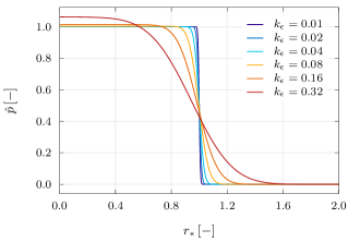
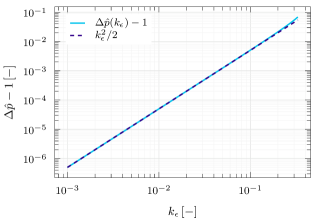
Figure 1: Exact pressure profiles for two-dimensional droplets with diffuse interface. On the left, the radial profile of the dimensionless pressure $\hat{p}=(p-p_{\mathrm{atm}})\,R/[(d-1)\,{\sigma}]$ is shown for a range of values of the interface thickness parameter $k_{\epsilon}$. On the right, we plot the error of the dimensionless pressure jump $\Delta\hat{p}$ of a smooth droplet with respect to the dimensionless Young–Laplace pressure jump (unity) as a function of the interface thickness parameter $k_{\epsilon}$. The dashed line represents a power law approximation of the curve.

2.4.1 Consistency with the Young–Laplace law.

In the limit of vanishing interface thickness ($k_{\epsilon}\rightarrow 0$), one can verify that Eq. (37) yields a pressure jump between atmospheric condition and the centre of the droplet of the form

$$\lim_{k_{\epsilon}\to 0}\Delta p(k_{\epsilon})=\lim_{k_{\epsilon}\to 0}\left[\left.p\left(r_{\ast}=0\right)\right|_{k_{\epsilon}}-p_{\mathrm{atm}}\right]=(d-1)\,\frac{\sigma}{R},$$ (38)

so that the well-known Young–Laplace formula is recovered in the limit of a sharp interface. Also, we can point out that, even for heavily smoothed droplets, the Young–Laplace formula provides similar values to the ones obtained from Eq. (37), as can be seen in the left panel of Figure 1, and that both estimates for the pressure jump converge to the same value quite quickly: from the right panel of Figure 1 it is apparent that the following approximation holds

$$\Delta p(k_{\epsilon})\simeq(d-1)\,\frac{\sigma}{R}\,\left(1+\frac{1}{2}\,k_{\epsilon}^{2}\right),$$ (39)

which means that the pressure jump is overall affected only by relatively small deviations from the Young–Laplace law, even for droplets with rather large diffuse interface region and converges to the sharp interface reference solution quadratically as the interface thickness $k_{\epsilon}$ vanishes

3 Numerical method

In this section, we summarise the key elements of the family of numerical methods employed in this work, which are the high order ADER Discontinuous Galerkin ($\mathbb{P}_{N}\mathbb{P}_{N}$) and ADER-WENO Finite Volume ($\mathbb{P}_{0}\mathbb{P}_{M}$) schemes with a posteriori subcell limiting. These methods can be applied to general nonconservative hyperbolic systems of balance laws. Discontinuous Galerkin schemes for nonconservative hyperbolic systems have been introduced in [45, 50, 130], following the path-conservative approach of Castro and Parés, originally developed for the Finite Volume framework [27, 116] and based on the theory of Dal Maso, Le Floch and Murat [102]. A recent review of the history of the development of ADER schemes can be found in [24]. For details on some of the first fully discrete one-step Lax-Wendroff-type time discretisations proposed for DG methods, see [128, 53, 99, 69].

Modern explicit ADER schemes follow a fully discrete predictor-corrector procedure, which can be regarded as a high order extension of the simple and successful MUSCL-Hancock approach [156, 157, 153], rather than using a semi-discrete formulation in conjunction with multi-stage timestepping, as in Runge–Kutta DG methods [29]. First, a predictor step evolves the polynomial data in the small to obtain an approximate space-time polynomial solution in each cell, without taking coupling with neighbouring cells into account. Then, volume integrals arising from a weak formulation of the differential problem can be easily evaluated with the aid of appropriate quadrature formulas, and quadrature at space-time faces are used to compute averaged numerical fluxes corresponding to the Riemann problems arising from extrapolation of the predictor solution from adjacent cells.

At each timestep, the cell-local space-time predictor solution $\bm{\mathrm{q}}_{h}(\bm{\mathrm{x}},\ t)$ is computed from a piecewise polynomial reconstruction $\bm{\mathrm{w}}_{h}(\bm{\mathrm{x}})$ of cell average data (for FV methods), or is directly available from the evolved piecewise polynomial data $\bm{\mathrm{w}}_{h}(\bm{\mathrm{x}})=\bm{\mathrm{u}}_{h}(\bm{\mathrm{x}})$ for DG methods. Since the two families of schemes (FV and DG) use the same discrete data representation (nodal degrees of freedom of a Gauss–Legendre–Lagrange polynomial), the space-time Discontinuous Galerkin predictor can be formulated in full generality for both, or even for the more general family of $\mathbb{P}_{N}\mathbb{P}_{M}$ schemes [42, 40].

From the space-time predictor solution one can immediately compute all the volume integrals appearing in the fully discrete, one-step update formulas (60); in particular, this operation can be carried out quite conveniently thanks to the choice of employing a nodal basis where the nodal values are located at the Gauss–Legendre quadrature nodes and the basis functions ${\phi_{m}(\bm{\mathrm{\xi}})={\psi_{m_{x}}}(\xi)\,{\psi_{m_{y}}}(\eta)\,{\psi_{m_{z}}}(\zeta)}$ are two-dimensional or three-dimensional tensor products of the Lagrange polynomials interpolating the Gauss–Legendre quadrature nodes.

In this work, spurious oscillations that typically occur when employing higher than first order linear schemes, see [73], are minimised as follows: in the case of Finite Volume methods, we employ a nonlinear WENO reconstruction procedure, while for Discontinuous Galerkin schemes we adopt the a posteriori subcell Finite Volume limiting strategy [59], that is, at each timestep a candidate solution is computed without any limiter, and then afterwards, if this candidate solution violates one or more physical and numerical admissibility criteria (floating point exceptions, violation of positivity, violation of a discrete maximum principle), then it is discarded and a new discrete solution is recomputed, starting again from valid data at the previous time step. This data is obtained by projecting the DG polynomial on a fine subcell grid, or directly from the subcell average representation of the data if it was already available at the previous timestep. Afterwards, the discrete solution is reconstructed back from subcell averages to a DG polynomial.

3.1 Data representation and notation

The computational domain is partitioned in conforming Cartesian elements

$$\Omega_{ijk}=\left[x_{i}-\frac{\Delta x_{i}}{2},\ x_{i}+\frac{\Delta x_{i}}{2}\right]\times\left[y_{j}-\frac{\Delta y_{j}}{2},\ y_{j}+\frac{\Delta y_{j}}{2}\right]\times\left[z_{k}-\frac{\Delta z_{k}}{2},\ z_{k}+\frac{\Delta z_{k}}{2}\right],$$ (40)

and for each element a reference frame of coordinates is defined by

$$\xi=\frac{x-x_{i}}{\Delta x_{i}}+\frac{1}{2},\qquad\eta=\frac{y-y_{j}}{\Delta y_{j}}+\frac{1}{2},\qquad\zeta=\frac{x-z_{k}}{\Delta z_{k}}+\frac{1}{2}.\qquad$$ (41)

Discrete data are given as the degrees of freedom of a $d$-dimensional polynomial (in this exposition we will use $d=3$ without loss of generality) represented by means of a set of nodal basis functions in the form of three-dimensional tensor products of the Lagrange polynomials ${\psi_{m_{x}}}(\xi)$, ${\psi_{m_{y}}}(\eta)$, and ${\psi_{m_{z}}}(\zeta)$ satisfying, at Gauss–Legendre quadrature node locations $\xi_{p_{x}}^{\textsc{gl}}$, $\eta_{p_{y}}^{\textsc{gl}}$, and $\zeta_{p_{z}}^{\textsc{gl}}$, the interpolation conditions ${\psi_{m_{x}}}(\xi_{p_{x}}^{\textsc{gl}})=\delta_{m_{x}\,p_{x}}$, ${\psi_{m_{y}}}(\eta_{p_{y}}^{\textsc{gl}})=\delta_{m_{y}\,p_{y}}$, and ${\psi_{m_{z}}}(\zeta_{p_{z}}^{\textsc{gl}})=\delta_{m_{z}\,p_{z}}$, with $\delta_{ij}$ being the usual Kronecker symbol.

Throughout the paper we will use a compact multi-index notation so that the three-dimensional position of the generic Gauss–Legendre quadrature node of index $p$ is written ${\bm{\mathrm{\xi}}_{p}^{\textsc{gl}}=(\xi_{p_{x}}^{\textsc{gl}},\ \eta_{p_{y}}^{\textsc{gl}},\ \zeta_{p_{z}}^{\textsc{gl}})}$ and the three dimensional basis function of index $m$ can be expressed as ${\phi_{m}(\bm{\mathrm{\xi}})={\psi_{m_{x}}}(\xi)\,{\psi_{m_{y}}}(\eta)\,{\psi_{m_{z}}}(\zeta)}$. Note that the interpolation property can be written in an entirely analogous fashion with respect to the one-dimensional case, that is, with the notation ${\phi_{m}(\bm{\mathrm{\xi}}_{p}^{\textsc{gl}})=\delta_{mp}}$.

Within each cell $\Omega_{ijk}$, at a given time $t=t^{n}$, the discrete solution is then written (dropping for convenience of notation the cell indices $i,j,k$) as a polynomial of order $M$ in each direction

$$\bm{\mathrm{u}}_{h}(\bm{\mathrm{x}},t^{n})=\bm{\mathrm{u}}_{h}(\bm{\mathrm{\xi}}(\bm{\mathrm{x}}),\ t^{n})=\sum_{m_{x}=1}^{M+1}\sum_{m_{y}=1}^{M+1}\sum_{m_{z}=1}^{M+1}{\psi_{m_{x}}}(\xi)\,{\psi_{m_{y}}}(\eta)\,{\psi_{m_{z}}}(\zeta)\,\hat{\bm{\mathrm{u}}}_{m_{x}\,m_{y}\,m_{z}}^{n}=\sum_{m=1}^{{(M+1)}^{d}}\phi_{m}(\bm{\xi})\,\hat{\bm{\mathrm{u}}}_{m}^{n}.$$ (42)

Furthermore, we will use the Einstein summation convention over repeated indices so that the discrete solution can be expressed as $\bm{\mathrm{u}}_{h}(\bm{\mathrm{x}},\ t^{n})=\phi_{m}(\bm{\mathrm{\xi}})\,\hat{\bm{\mathrm{u}}}_{m}^{n}$. The Finite Volume data representation (cell average values ${\bm{\mathrm{Q}}}_{ijk}^{n})$ can be regarded as a special case of (42) in which $M=0$ and the single basis function is the constant function $\phi_{m}^{\textsc{fv}}(\bm{\mathrm{\xi}})=1$ within each element.

3.2 Polynomial WENO reconstruction

In order to obtain a high order data reconstruction from Finite Volume cell averages, we employ a full polynomial WENO reconstruction, introduced in [51] for unstructured meshes and employed, for example, in [58] on Cartesian grids. The most prominent difference between this approach and the original formulation by Jiang and Shu [89] is that instead of computing pointwise values of the conserved variables at the aid of optimal linear weights, here we seek to obtain the degrees of freedom of the entire reconstruction polynomial, to be used in the computation of fluxes, non-conservative products and source terms via high order quadrature formulae. At this point we would also like to stress that entire WENO reconstruction polynomials with a reconstruction stencil of optimal compactness can be achieved via the elegant CWENO approach forwarded by Puppo, Russo and Semplice et al  in [96, 97, 142, 32, 44]. The first step is to define, for a generic element $\Omega_{ijk}=[x_{i-{1}/{2}},\ x_{i+{1}/{2}}]\times[y_{j-{1}/{2}},\ y_{j+{1}/{2}}]\times[z_{k-{1}/{2}},\ z_{k+{1}/{2}}]$, the three sets of reconstruction stencils, one for each space dimension. Each stencil will be identified by the triplet of subscripts ($i,\ j,\ k$) of the cell in which the reconstruction is sought, together with the superscript describing the spatial direction ($x$, $y$ or $z$) of the reconstruction and an integer superscript $s$ that identifies the specific stencil in the set. The three generic elements of such reconstruction stencil sets will be then written as

$$S_{ijk}^{x,\,s}=\bigcup_{m=i-L}^{i+R}\Omega_{mjk},\qquad S_{ijk}^{y,\,s}=\bigcup_{m=j-L}^{j+R}\Omega_{imk},\qquad S_{ijk}^{z,\,s}=\bigcup_{m=k-L}^{k+R}\Omega_{ijm},\qquad$$ (43)

where $L=L(M,\ s)$ and $R=R(M,\ s)$ are positive integers representing the number of elements in the stencil respectively to the left and to the right of the principal cell. In each space direction, for even values of the the reconstruction degree $M$, one always has $N_{\mathrm{s}}=3$ stencils, one central and two off-centre, with left and right extensions given by

$$L(M,\ s)=\begin{cases}M/2&\text{if }s=1,\\ M&\text{if }s=2,\\ 0&\text{if }s=3,\\ \end{cases}\qquad R(M,\ s)=\begin{cases}M/2&\text{if }s=1,\\ 0&\text{if }s=2,\\ M&\text{if }s=3,\\ \end{cases}\qquad$$ (44)

while for odd values of $M$ we define $N_{\mathrm{s}}=4$ types of stencils, two central, two off-centre, having extensions

$$L(M,\ s)=\begin{cases}(M+1)/2&\text{if }s=1,\\ (M-1)/2&\text{if }s=2,\\ M&\text{if }s=3,\\ 0&\text{if }s=4,\\ \end{cases}\qquad R(M,\ s)=\begin{cases}(M-1)/2&\text{if }s=1,\\ (M+1)/2&\text{if }s=2,\\ 0&\text{if }s=3,\\ M&\text{if }s=4.\\ \end{cases}\qquad$$ (45)

This choice ensures that each stencil be composed by a number of elements equal to the nominal order of the scheme, which is $M+1$.

The dimension-by-dimension reconstruction is carried out by repeated application (over each space dimension) of a one-dimensional-sweep procedure which constructs, in each cell, the $M+1$ degrees of freedom of a polynomial of degree $M$, first solving a set of linear reconstruction equations (imposing conservation of cell averages on each element of a given stencil), and then combining the solutions of the reconstruction equations in a data-dependent, nonlinear fashion in order to ensure the non-oscillatory character of the reconstructed polynomials.

In the generic element $\Omega_{ijk}$, the reconstruction polynomials obtained in each of the three subsequent passes are expressed in terms of their degrees of freedom $\hat{\bm{\mathrm{w}}}^{\textsc{1d}}_{i\,j\,k,\,p}$, $\hat{\bm{\mathrm{w}}}^{\textsc{2d}}_{i\,j\,k,\,p\,q}$, and $\hat{\bm{\mathrm{w}}}^{\textsc{3d}}_{i\,j\,k,\,p\,q\,r}$, relative to a tensor-product-type Gauss–Legendre–Lagrange basis function. The degrees of freedom and thus the polynomials are obtained as nonlinear convex combinations, written as

$$\bm{\mathrm{w}}_{h}^{\textsc{1d}}(x)=\psi_{p}(\xi)\,\hat{\bm{\mathrm{w}}}^{\textsc{1d}}_{ijk,\,p}, \text{with}\quad\hat{\bm{\mathrm{w}}}^{\textsc{1d}}_{ijk,\,p}=\omega_{s}^{\textsc{1d}}\,\hat{\bm{\mathrm{w}}}^{\textsc{1d},\,s}_{ijk,\,p},$$ (46)

$$\bm{\mathrm{w}}_{h}^{\textsc{2d}}(x,y)=\psi_{p}(\xi)\,\psi_{q}(\eta)\,\hat{\bm{\mathrm{w}}}^{\textsc{2d}}_{ijk,\,pq}, \text{with}\quad\hat{\bm{\mathrm{w}}}^{\textsc{2d}}_{ijk,\,pq}=\omega_{s}^{\textsc{2d}}\,\hat{\bm{\mathrm{w}}}^{\textsc{2d},\,s}_{ijk,\,pq},$$ (47)

$$\bm{\mathrm{w}}_{h}^{\textsc{3d}}(x,y,z)=\psi_{p}(\xi)\,\psi_{q}(\eta)\,\psi_{r}(\zeta)\,\hat{\bm{\mathrm{w}}}^{\textsc{3d}}_{ijk,\,pqr}, \text{with}\quad\hat{\bm{\mathrm{w}}}^{\textsc{3d}}_{ijk,\,pqr}=\omega_{s}^{\textsc{3d}}\,\hat{\bm{\mathrm{w}}}^{\textsc{3d},\,s}_{ijk,\,pqr},$$ (48)

having defined, for each stencil $S_{ijk}^{x,\,s}$, $S_{ijk}^{y,\,s}$, and, $S_{i\,j\,k}^{z,\,s}$ the linear (in the sense that they are not affected by limiting) reconstruction polynomials computed from the solution of the reconstruction equations

$$\bm{\mathrm{w}}_{h}^{\textsc{1d},\,s}(x)=\psi_{p}(\xi)\,\hat{\bm{\mathrm{w}}}_{ijk,\,p}^{\textsc{1d},\,s},$$ (49)

$$\bm{\mathrm{w}}_{h}^{\textsc{2d},\,s}(x,y)=\psi_{p}(\xi)\,\psi_{q}(\eta)\,\hat{\bm{\mathrm{w}}}_{i\,j\,k,\,p\,q}^{\textsc{2d},\,s},$$ (50)

$$\bm{\mathrm{w}}_{h}^{\textsc{3d},\,s}(x,y,z)=\psi_{p}(\xi)\,\psi_{q}(\eta)\,\psi_{r}(\zeta)\,\hat{\bm{\mathrm{w}}}_{ijk,\,pqr}^{\textsc{3d},\,s},$$ (51)

where the indices $p$, $q$, and $r$ run from $0$ to $M$ (covering the number of degrees of freedom to be reconstructed in the in each space dimension) and where we adopted Einstein’s summation convention over repeated indices.

Each pass is analogous to the first one, in that a one-dimensional stencil is used and only a one-dimensional oscillation indicator has to be computed, but it must be remarked that, as a result of performing the nonlinear stencil selection procedure in a given dimension before operating the linear reconstructions in the next one, each one of the final three-dimensional degrees of freedom is subject to composite limiting in the three space dimensions, which includes information not only from the direct face neighbours, but from the node neighbours as well, and the reconstruction is thus genuinely multi-dimensional. For alternative and more efficient multi-dimensional finite volume WENO reconstructions on Cartesian meshes, see [23, 22].

More in detail, first, one constructs for each cell a one-dimensional polynomial $\bm{\mathrm{w}}_{h}^{\textsc{1d}}(x)$, while maintaining the data in the remaining directions ($y$ and $z$) in piecewise constant cell-averaged form.

The linear reconstruction equations, enforcing integral conservation on all elements in the stencil $S_{ijk}^{x,\,s}$, constitute a linear system whose solutions are the $M+1$ unknown degrees of freedom $\hat{\bm{\mathrm{w}}}_{ijk,\,p}^{1\textsc{d},s}$, and in the first space dimension read

$$\dfrac{1}{\Delta x_{m}}\int_{x_{m-\frac{1}{2}}}^{x_{m+\frac{1}{2}}}\psi_{p}(\xi(x))\,\hat{\bm{\mathrm{w}}}^{\textsc{1d},\,s}_{ijk,\,p}\,\operatorname{d\!}{x}={\bm{\mathrm{Q}}}_{mjk}^{n},\quad\forall\,\Omega_{mjk}\in S_{ijk}^{x,\,s}.$$ (52)

Then the nonlinear coefficients for the combination of the polynomials obtained from each stencil are computed at each line sweep as

$$\omega_{s}^{n\textsc{d}}=\tilde{\omega}_{s}^{n\textsc{d}}\,{\left(\sum_{s=1}^{N_{s}}\tilde{\omega}_{s}^{n\textsc{d}}\right)}^{-1},\quad\text{with}\quad\tilde{\omega}_{s}^{n\textsc{d}}=\lambda_{s}\,{\left(\sigma_{s}^{n\textsc{d}}+\epsilon\right)}^{-r},$$ (53)

where the oscillation indicator $\sigma_{s}^{n\textsc{d}}$ is defined as

$$\sigma_{s}^{n\textsc{d}}=\sum_{l=0}^{M}\sum_{m=0}^{M}\Sigma_{l\,m}\,\frac{\hat{\bm{\mathrm{w}}}_{ijk,\,l}^{n\textsc{d},\,s}}{\bm{\mathrm{w}}_{0}}\,\frac{\hat{\bm{\mathrm{w}}}_{ijk,\,m}^{n\textsc{d},\,s}}{\bm{\mathrm{w}}_{0}},\quad\text{with}\quad\Sigma_{l\,m}=\sum_{\alpha=1}^{M}\int_{0}^{1}\dfrac{\partial^{\alpha}\psi_{l}(\xi)}{\partial\xi^{\alpha}}\,\dfrac{\partial^{\alpha}\psi_{m}(\xi)}{\partial\xi^{\alpha}}\operatorname{d\!}{\xi}.$$ (54)

The numerical parameters used for the computation of the nonlinear weights are $\lambda_{s}=1$ for off-centre stencils and $\lambda_{s}=10^{5}$ for central stencils, and we set $\epsilon=10^{-14}$ and $r=8$. An important remark is that since the oscillation indicators are highly nonlinear, particular care should be taken in dividing the input values by an appropriate scaling factor $\bm{\mathrm{w}}_{0}$. As a practical example, it is often the case that when using the stiffened gas equation of state, very large values for the mixture energy variable appear even in standard pressure conditions, which could lead to catastrophic loss of precision in the computation of the weights. Such a scaling factor can be computed for example as

$$\bm{\mathrm{w}}_{0}=\epsilon_{0}+\sum_{s}\sum_{m=0}^{M}\left|\hat{\bm{\mathrm{w}}}_{ijk,\,m}^{n\textsc{d},\,s}\right|,$$ (55)

that is, by evaluating, variable by variable, the sum of the absolute values of all the degrees of freedom of the input data over all stencils and adding a new constant $\epsilon_{0}=10^{-14}$ to avoid division by zero.

In the second pass, one obtains data in the two-dimensional polynomial form $\bm{\mathrm{w}}_{h}^{\textsc{2d},\,s}(x,\ y)$, by first solving

$$\dfrac{1}{\Delta y_{m}}\int_{y_{m-\frac{1}{2}}}^{y_{m+\frac{1}{2}}}\psi_{q}(\eta(y))\,\hat{\bm{\mathrm{w}}}^{\textsc{2d},\,s}_{ijk,\,pq}\,\operatorname{d\!}{y}=\hat{\bm{\mathrm{w}}}^{\textsc{1d}}_{imk,\,p},\quad\forall\,\Omega_{imk}\in S_{ijk}^{y,\,s},$$ (56)

for each degree of freedom $\hat{\bm{\mathrm{w}}}^{\textsc{1d}}_{imk,\,p}$ and then carrying out the nonlinear selection as in the first pass. Analogously, in the third space dimension, conservation over each element of the stencil gives

$$\dfrac{1}{\Delta z_{m}}\int_{z_{m-\frac{1}{2}}}^{z_{m+\frac{1}{2}}}\psi_{r}(\zeta(z))\,\hat{\bm{\mathrm{w}}}^{\textsc{3d},\,s}_{ijk,\,pqr}\,\operatorname{d\!}{z}=\hat{\bm{\mathrm{w}}}^{\textsc{2d}}_{ijm,\,pq},\quad\forall\,\Omega_{ijm}\in S_{ijk}^{z,\,s},$$ (57)

to be solved once for each degree of freedom $\hat{\bm{\mathrm{w}}}^{\textsc{2d}}_{ijm,\,pq}$, and finally one obtains the sought three-dimensional weighted essentially-non-oscillatory polynomial after the nonlinear combination of the individual stencil polynomials has been applied.

3.3 Reconstruction in primitive variables

In this work, we employ a primitive variable reconstruction in order to better treat some of the peculiar issues that are typically encountered in the numerical solution of multiphase flow models, namely the presence of a complex, volume fraction-dependent equation of state and/or other issues due to different material interfaces evolving separately, already reported in [1] and [94]: this separation between interfaces might give rise to nonphysical discontinuities in the velocity and density fields as well as positivity violations in the mass fraction. The use of a primitive variable reconstruction for the TVD second order MUSCL-Hancock scheme, or the ADER-WENO $\mathbb{P}_{0}\mathbb{P}_{2}$ scheme used in the troubled elements as subcell limiter schemes was found to significantly mitigate these problems.

The primitive variable reconstruction procedure used for the ADER-WENO $\mathbb{P}_{0}\mathbb{P}_{2}$ limiter was introduced in [163], along with a predictor step formulated in terms of the primitive form of the governing equations. The reconstruction is performed as follows: first, a conservative polynomial WENO reconstruction is computed and the polynomials obtained from this step are evaluated at the cell centres so to obtain high order accurate point values for the conserved variables. Then one can convert the point values of conserved variables to primitive variables and perform a second WENO reconstruction to achieve a high order polynomial reconstruction of the primitive data. This second reconstruction step repeats the same steps described in Section 3.2, with the difference that the reconstruction equations are not based on directly enforcing conservation on a stencil, but rather they are obtained by requiring that the primitive variable reconstruction polynomials interpolate the cell centre value where the conversion from conserved to primitive variables has taken place. For alternative high order WENO reconstructions in primitive variables, see [13, 122].

3.4 One-step, fully discrete, explicit update formulas

We consider a general nonconservative hyperbolic system written as

$$\partial_{t}\bm{\mathrm{Q}}+\nabla\cdot\bm{\mathrm{F}}(\bm{\mathrm{Q}})+\bm{\mathrm{B}}(\bm{\mathrm{Q}})\cdot\nabla\bm{\mathrm{Q}}=\bm{\mathrm{S}}(\bm{\mathrm{Q}}).$$ (58)

in a space time control volume $\Omega_{ijk}\times[t_{n},\ t_{n+1}]$; we then define the differential volume element $\operatorname{d\!}{\bm{\mathrm{x}}}=\operatorname{d\!}{x}\,\operatorname{d\!}{y}\,\operatorname{d\!}{z}$ for compactly writing integrals over the control volume $\Omega_{ijk}$ and the surface element $\operatorname{d\!}{\bm{\mathrm{s}}}$ for compactly writing integrals over its boundary $\partial\Omega_{ijk}$. By multiplying each term of the PDE (58) with a test function $\phi_{p}$, formally integrating over the space-time element and applying Gauss’s theorem for integrating the divergence of fluxes in space, we have a weak formulation

$$\int\limits_{t_{n}}^{t_{n+1}}\int\limits_{\Omega_{ijk}}\phi_{p}\,\partial_{t}\bm{\mathrm{Q}}\,\operatorname{d\!}{\bm{\mathrm{x}}}\,\operatorname{d\!}{t}+\int\limits_{t_{n}}^{t_{n+1}}\int\limits_{\partial\Omega_{ijk}}\phi_{p}\,\bm{\mathrm{F}}(\bm{\mathrm{Q}})\cdot\bm{\mathrm{\hat{n}}}\,\operatorname{d\!}{\bm{\mathrm{s}}}\,\operatorname{d\!}{t}\ -\int\limits_{t_{n}}^{t_{n+1}}\int\limits_{\Omega_{ijk}}\nabla\phi_{p}\cdot\bm{\mathrm{F}}(\bm{\mathrm{Q}})\,\operatorname{d\!}{\bm{\mathrm{x}}}\,\operatorname{d\!}{t}\ +$$ (59)

$$+\int\limits_{t_{n}}^{t_{n+1}}\int\limits_{\Omega_{ijk}}\phi_{p}\,\left[\bm{\mathrm{B}}(\bm{\mathrm{Q}})\cdot\nabla\bm{\mathrm{Q}}-\bm{\mathrm{S}}(\bm{\mathrm{Q}})\right]\,\operatorname{d\!}{\bm{\mathrm{x}}}\,\operatorname{d\!}{t}=\bm{\mathrm{0}},$$

with $\bm{\mathrm{\hat{n}}}$ defined as the outward unit normal vector on the element boundary. Then, by substituting the sought polynomial solution $\bm{\mathrm{u}}_{h}(\bm{\mathrm{x}},t^{n})=\phi_{m}(\bm{\mathrm{\xi}})\,\hat{\bm{\mathrm{u}}}_{m}^{n}$, as well as the polynomials $\bm{\mathrm{q}}_{h}(\bm{\mathrm{x}},t)=\theta_{m}(\bm{\mathrm{\xi}},\tau)\,\hat{\bm{\mathrm{q}}}_{m}$ obtained from the local space-time predictor detailed in the next section, we have the fully-discrete one-step update formula

$$\left(\,\int\limits_{\Omega_{ijk}}\phi_{p}\,\phi_{q}\operatorname{d\!}{\bm{\mathrm{x}}}\right)\,\left(\hat{\bm{\mathrm{u}}}_{q}^{n+1}-\hat{\bm{\mathrm{u}}}_{q}^{n}\right)+\int\limits_{t_{n}}^{t_{n+1}}\int\limits_{\partial\Omega_{ijk}}\phi_{p}\,\bm{\mathrm{F}}_{\textsc{rp}}\left(\bm{\mathrm{q}}_{h}^{\textsc{l}},\ \bm{\mathrm{q}}_{h}^{\textsc{r}}\right)\cdot\bm{\mathrm{\hat{n}}}\,\operatorname{d\!}{\bm{\mathrm{s}}}\,\operatorname{d\!}{t}\int\limits_{t_{n}}^{t_{n+1}}\int\limits_{\partial\Omega_{ijk}}\phi_{p}\,\bm{\mathrm{D}}_{\Psi}\left(\bm{\mathrm{q}}_{h}^{\textsc{l}},\ \bm{\mathrm{q}}_{h}^{\textsc{r}}\right)\cdot\bm{\mathrm{\hat{n}}}\,\operatorname{d\!}{\bm{\mathrm{s}}}\,\operatorname{d\!}{t}\ +$$ (60)

$$-\int\limits_{t_{n}}^{t_{n+1}}\int\limits_{\Omega_{ijk}^{\circ}}\nabla\phi_{p}\cdot\bm{\mathrm{F}}(\bm{\mathrm{q}}_{h})\,\operatorname{d\!}{\bm{\mathrm{x}}}\,\operatorname{d\!}{t}+\int\limits_{t_{n}}^{t_{n+1}}\int\limits_{\Omega_{ijk}^{\circ}}\phi_{p}\,\left[\bm{\mathrm{B}}(\bm{\mathrm{q}}_{h})\cdot\nabla\bm{\mathrm{q}}_{h}-\bm{\mathrm{S}}(\bm{\mathrm{q}}_{h})\right]\,\operatorname{d\!}{\bm{\mathrm{x}}}\,\operatorname{d\!}{t}=\bm{\mathrm{0}},$$

where we denoted with $\bm{\mathrm{F}}_{\textsc{rp}}$ the generic numerical flux function, that would be, for this work, the Rusanov flux (74) or the HLL flux (71), but also other approximate Riemann solvers could be used, such as the generalized Osher and HLLEM methods forwarded in [57, 41]. Analogously, we define the path-conservative fluctuation term as

$$\bm{\mathrm{D}}_{\Psi}\left(\bm{\mathrm{q}}_{h}^{\textsc{l}},\ \bm{\mathrm{q}}_{h}^{\textsc{r}}\right)\cdot\bm{\mathrm{\hat{n}}}=\omega\,\int_{0}^{1}\bm{\mathrm{B}}\left[\Psi\left(\bm{\mathrm{q}}_{h}^{\textsc{l}},\ \bm{\mathrm{q}}_{h}^{\textsc{r}},\ s\right)\right]\cdot\bm{\mathrm{\hat{n}}}\,\operatorname{d\!}{s}\,\left(\bm{\mathrm{q}}_{h}^{\textsc{r}}-\bm{\mathrm{q}}_{h}^{\textsc{l}}\right),\quad\text{with}\quad\Psi\left(\bm{\mathrm{q}}_{h}^{\textsc{l}},\ \bm{\mathrm{q}}_{h}^{\textsc{r}},\ s\right)=\bm{\mathrm{q}}_{h}^{\textsc{l}}+s\,(\bm{\mathrm{q}}_{h}^{\textsc{r}}-\bm{\mathrm{q}}_{h}^{\textsc{l}}),$$ (61)

in which $\Psi\left(\bm{\mathrm{q}}_{h}^{\textsc{l}},\ \bm{\mathrm{q}}_{h}^{\textsc{r}},\ s\right)$ is a simple segment path function connecting the left and right states, and the path integral can be computed with a three-point Gauss–Legendre quadrature regardless of the order of the scheme. The coefficients $\omega$ must be chosen so to enforce the consistency condition [27, 116]

$$\bm{\mathrm{D}}_{\Psi}\left(\bm{\mathrm{q}}_{h}^{\textsc{l}},\ \bm{\mathrm{q}}_{h}^{\textsc{r}}\right)\cdot\bm{\mathrm{\hat{n}}} -\bm{\mathrm{D}}_{\Psi}\left(\bm{\mathrm{q}}_{h}^{\textsc{r}},\ \bm{\mathrm{q}}_{h}^{\textsc{l}}\right)\cdot\bm{\mathrm{\hat{n}}}=\int_{0}^{1}\bm{\mathrm{B}}\left[\Psi\left(\bm{\mathrm{q}}_{h}^{\textsc{l}},\ \bm{\mathrm{q}}_{h}^{\textsc{r}},\ s\right)\right]\cdot\bm{\mathrm{\hat{n}}}\,\frac{\raisebox{0.0pt}{$\partial\Psi$}}{\vphantom{l^{l}}\partial s}\,\operatorname{d\!}{s}\,$$ (62)

and simple expressions are provided in Sections 3.5.2 and 3.5.3 for the HLL and Rusanov fluxes. The inversion of the mass matrix integrating the products $\phi_{p}\,\phi_{q}$ is trivial, as the choice of basis yields an orthogonal basis and thus a diagonal mass matrix. The volume integrals appearing in (60) may be directly evaluated by Gauss–Legendre quadrature using the nodes on which the degrees of freedom of the space-time predictor solution $\bm{\mathrm{q}}_{h}$ are defined, while for face integrals one has to extrapolate $\bm{\mathrm{q}}_{h}^{\textsc{l}}$ and $\bm{\mathrm{q}}_{h}^{\textsc{r}}$ from two adjacent cells onto the Gauss–Legendre quadrature nodes at a face, then evaluate the two-state numerical fluxes at each one of the quadrature nodes, and finally operate the weighted sum of all the numerical fluxes.

Since numerical flux functions can be in principle computationally quite expensive, an attractive alternative choice for the integration of fluxes at space-time cell boundaries, with respect to the tensor-product quadrature rule, is the following: during the space-time predictor step, automatically a polynomial approximation of the physical fluxes $\bm{\mathrm{f}}_{h}=\bm{\mathrm{f}}{(\bm{\mathrm{q}}_{h})}$ is computed within each cell. When performing the extrapolation of $\bm{\mathrm{q}}_{h}^{\textsc{l}}$ and $\bm{\mathrm{q}}_{h}^{\textsc{r}}$ to the space-time boundaries, one may also directly extrapolate the approximation of the physical fluxes to the boundaries, obtaining thus at each space-time cell boundary $\bm{\mathrm{f}}_{h}^{\textsc{l}}$ and $\bm{\mathrm{f}}_{h}^{\textsc{r}}$.

Here we denoted with $\bm{\mathrm{f}}$ the projection of the physical flux tensor $\bm{\mathrm{F}}$ on one of the three canonical basis vectors indicating the orientation of the face-normal onto which the flux is to be extrapolated, that is $\bm{\mathrm{f}}=\bm{\mathrm{F}}\cdot\bm{\mathrm{\hat{e}}}_{x}$, $\bm{\mathrm{g}}=\bm{\mathrm{F}}\cdot\bm{\mathrm{\hat{e}}}_{y}$, or $\bm{\mathrm{h}}=\bm{\mathrm{F}}\cdot\bm{\mathrm{\hat{e}}}_{z}$ in the first, second, or third direction, respectively.

Then one can treat $\bm{\mathrm{q}}_{h}^{\textsc{l}}$, $\bm{\mathrm{q}}_{h}^{\textsc{r}}$, $\bm{\mathrm{f}}_{h}^{\textsc{l}}$, and $\bm{\mathrm{f}}_{h}^{\textsc{r}}$ as four independent variables and recognise that the numerical fluxes employed in the present work can be seen, if wavespeed estimates are considered fixed, as split into a centred part (solely function of $\bm{\mathrm{f}}_{h}^{\textsc{l}}$ and $\bm{\mathrm{f}}_{h}^{\textsc{r}}$) and a diffusive part (function of $\bm{\mathrm{q}}_{h}^{\textsc{l}}$ and $\bm{\mathrm{q}}_{h}^{\textsc{r}}$). Moreover, such a four-variable numerical flux with fixed wavespeed estimates is linear in its arguments and in order to exploit this property, the coefficients may be evaluated only once at a space-time-face-averaged state and employed for all space-time face integration points. Thanks to the simple choice of a linear segment path, one can apply the same approach to the computation of the path integral of nonconservative products, and compute the average nonconservative product coefficient matrix

$$\bm{\mathrm{B}}_{\bm{\mathrm{\Psi}}}=\int_{0}^{1}\bm{\mathrm{B}}\left[\Psi\left(\bm{\mathrm{q}}_{h}^{\textsc{l}},\ \bm{\mathrm{q}}_{h}^{\textsc{r}},\ s\right)\right]\cdot\bm{\mathrm{\hat{n}}}\,\operatorname{d\!}{s}$$ (63)

only once, integrating between the averaged states at the two faces, then multiplying (63) by the two weights $\omega_{LR}$ and $\omega_{RL}$ and by the space-time-face average jump between $\bm{\mathrm{q}}_{h}^{\textsc{l}}$ and $\bm{\mathrm{q}}_{h}^{\textsc{r}}$, yielding $\bm{\mathrm{D}}_{\Psi}\left(\bm{\mathrm{q}}_{h}^{\textsc{l}},\ \bm{\mathrm{q}}_{h}^{\textsc{r}}\right)\cdot\bm{\mathrm{\hat{n}}}$ and $\bm{\mathrm{D}}_{\Psi}\left(\bm{\mathrm{q}}_{h}^{\textsc{r}},\ \bm{\mathrm{q}}_{h}^{\textsc{l}}\right)\cdot\bm{\mathrm{\hat{n}}}$, respectively.

This means that only one nonlinear computation of the wavespeed estimates and other nonlinearities in the Riemann solver has to be performed (with the face-averaged state of $\bm{\mathrm{q}}_{h}$), while the central part of the flux can be integrated directly, as well as the jump term in conserved variables. An added benefit of this approach is that the scheme need not to retain information regarding the space-time degrees of freedom of the predictor solution, making it possible and easy to implement low-storage schemes that are of uniform arbitrary high order in space and time.

Finally, in order to guarantee stability of the explicit timestepping, in this work we restrict the timestep size by

$$\Delta t=\textsc{CFL}\,\frac{k_{N}\min{(\Delta x,\ \Delta y,\ \Delta z)}}{d\,\lambda_{\mathrm{max}}},$$ (64)

with $N$ being the degree of the piecewise polynomial data representation, $d$ the number of space dimensions, and $\lambda_{\mathrm{max}}$ the maximum absolute value of all eigenvalues found in the domain (more specifically, searching over all the quadrature nodes, i.e. where the degrees of freedom of the nodal basis are collocated). With $\textsc{CFL}\leq 1$ we denote a Courant-type number that is typically chosen as $\textsc{CFL}=0.9$ for all the simulations presented in this work. The function $k_{N}$ was defined by numerical Von Neumann stability analysis in [42] for polynomials of degree up to four, while for higher values of $N$, we refer to an experimental determination based on numerical tests with linear advection.

The first five values of $k_{N}$ are $1.0$, $0.33$, $0.17$, $0.10$, and $0.069$ starting from Finite Volume ($N=0$) up to $N=4$ (fifth order $\mathbb{P}_{4}\mathbb{P}_{4}$ ADER-DG scheme), while for $5\leq N\leq 9$ we choose, $k_{N}$ from the vector $k_{5-9}={[0.045,\ 0.038,\ 0.03,\ 0.02,\ 0.01]}^{\mathsf{T}}$. We conclude by pointing out that condition (64) follows the same behaviour of the common $\Delta t_{\mathrm{max}}\sim 1/(2\,N+1)$ hyperbola for RKDG methods, but is slightly more restrictive.

3.5 Space-time Discontinuous Galerkin predictor

We now describe the procedure to obtain the space-time predictor polynomials, which are defined as

$$\bm{\mathrm{q}}_{h}(\xi,\eta,\zeta,\tau)={\psi_{m_{x}}}(\xi)\,{\psi_{m_{y}}}(\eta)\,{\psi_{m_{z}}}(\zeta)\,{\psi_{m_{t}}}(\tau)\,\hat{\bm{\mathrm{q}}}_{m_{x}\,m_{y}\,m_{z}\,m_{t}}=\theta_{m}(\xi,\eta,\zeta,\tau)\,\hat{\bm{\mathrm{q}}}_{m},$$ (65)

again formally allowing referencing to the components of $\theta$ with mono-indexing or multi-indexing. The first step for the local time evolution starting from the polynomial data $\bm{\mathrm{w}}_{h}(\bm{\mathrm{x}},\ t^{n})$ is to write the governing PDE (16) in a weak integral form in space and time as

$$\int\limits_{t_{n}}^{t_{n+1}}\int\limits_{\Omega_{ijk}}\theta_{p}\,\partial_{t}\bm{\mathrm{q}}_{h}\,\operatorname{d\!}{\bm{\mathrm{x}}}\,\operatorname{d\!}{t}+\int\limits_{t_{n}}^{t_{n+1}}\int\limits_{\Omega_{ijk}}\theta_{p}\,\nabla\cdot\bm{\mathrm{F}}(\bm{\mathrm{q}}_{h})\,\operatorname{d\!}{\bm{\mathrm{x}}}\,\operatorname{d\!}{t}+\int\limits_{t_{n}}^{t_{n+1}}\int\limits_{\Omega_{ijk}}\theta_{p}\,\left[\bm{\mathrm{B}}(\bm{\mathrm{q}}_{h})\cdot\nabla\bm{\mathrm{q}}_{h}-\bm{\mathrm{S}}(\bm{\mathrm{q}}_{h})\right]\,\operatorname{d\!}{\bm{\mathrm{x}}}\,\operatorname{d\!}{t}=0,$$ (66)

and then integrating by parts in time the first term (and by upwinding in time the value of $\bm{\mathrm{q}}_{h}(\bm{\mathrm{x}},\ t^{n})$ from the reconstruction polynomial $\bm{\mathrm{w}}_{h}(\bm{\mathrm{x}},t^{n})$), we can write

$$\phantom{+}\int\limits_{\Omega_{ijk}}\theta_{p}(\bm{\mathrm{x}},\ t^{n+1})\,\bm{\mathrm{q}}_{h}(\bm{\mathrm{x}},\ t^{n+1})\,\operatorname{d\!}{\bm{\mathrm{x}}}-\int\limits_{\Omega_{ijk}}\theta_{p}(\bm{\mathrm{x}},\ t^{n})\,\bm{\mathrm{w}}_{h}(\bm{\mathrm{x}},\ t^{n})\,\operatorname{d\!}{\bm{\mathrm{x}}}-\int\limits_{t_{n}}^{t_{n+1}}\int\limits_{\Omega_{ijk}}\partial_{t}\theta_{p}\,\bm{\mathrm{q}}_{h}\,\operatorname{d\!}{\bm{\mathrm{x}}}\,\operatorname{d\!}{t}\ +$$ (67)

$$+\int\limits_{t_{n}}^{t_{n+1}}\int\limits_{\Omega_{ijk}}\theta_{p}\,\nabla\cdot\bm{\mathrm{F}}(\bm{\mathrm{q}}_{h})\,\operatorname{d\!}{\bm{\mathrm{x}}}\,\operatorname{d\!}{t}+\int\limits_{t_{n}}^{t_{n+1}}\int\limits_{\Omega_{ijk}}\theta_{p}\,\bm{\mathrm{B}}(\bm{\mathrm{q}}_{h})\cdot\nabla\bm{\mathrm{q}}_{h}\,\operatorname{d\!}{\bm{\mathrm{x}}}\,\operatorname{d\!}{t}=\int\limits_{t_{n}}^{t_{n+1}}\int\limits_{\Omega_{ijk}}\theta_{p}\,\bm{\mathrm{S}}(\bm{\mathrm{q}}_{h})\,\operatorname{d\!}{\bm{\mathrm{x}}}\,\operatorname{d\!}{t}.$$

By then substituting the ansatz (65) in (67) one obtains a system of ${(M+1)}^{d+1}$ nonlinear algebraic equations which one can solve by means of a discrete Picard iteration with appropriate initial guess, as discussed in [46, 48, 24].

3.5.1 Predictor step in primitive variables

In conjunction with the primitive variable WENO reconstruction described in Section 3.2, as well as for pure ADER Discontinuous Galerkin schemes, for which primitive variable polynomials can be obtained by simply evaluating the primitive state vector in correspondence of each quadrature node location (nodal degree of freedom), we also carry out the local time evolution procedure with a primitive variable formulation, as per the methodology introduced in [163]. This variant of the local space-time predictor step is based on a primitive variable version of the governing equations, which directly evolves the primitive state vector $\bm{\mathrm{V}}$, uses only gradients of the primitive variables $\nabla\bm{\mathrm{V}}$ and is recovered by applying the chain rule to the governing equations in the form (58) to obtain

$$\frac{\raisebox{0.0pt}{$\partial\bm{\mathrm{V}}$}}{\vphantom{l^{l}}\partial t}+{\left(\frac{\raisebox{0.0pt}{$\partial\bm{\mathrm{Q}}$}}{\vphantom{l^{l}}\partial\bm{\mathrm{V}}}\right)}^{-1}\left(\frac{\raisebox{0.0pt}{$\partial\bm{\mathrm{F}}$}}{\vphantom{l^{l}}\partial\bm{\mathrm{V}}}+\bm{\mathrm{B}}\cdot\frac{\raisebox{0.0pt}{$\partial\bm{\mathrm{Q}}$}}{\vphantom{l^{l}}\partial\bm{\mathrm{V}}}\right)\cdot\nabla\bm{\mathrm{V}}={\left(\frac{\raisebox{0.0pt}{$\partial\bm{\mathrm{Q}}$}}{\vphantom{l^{l}}\partial\bm{\mathrm{V}}}\right)}^{-1}\bm{\mathrm{S}},$$ (68)

We now assign the notation $\bm{\mathrm{w}}_{h}^{\ast}$ to represent the discrete reconstruction data in primitive variables, obtained either by the primitive variable WENO reconstruction, or by a straightforward conversion of the nodal degrees of freedom for ADER-DG schemes, and define $\bm{\mathrm{v}}_{h}$ to be the discrete space-time predictor solution in primitive variables, we can write a weak form of the governing equations as

$$\int\limits_{t_{n}}^{t_{n+1}}\int\limits_{\Omega_{ijk}}\theta_{l}\,\partial_{t}\bm{\mathrm{v}}_{h}\,\operatorname{d\!}{\bm{\mathrm{x}}}\,\operatorname{d\!}{t}+\int\limits_{t_{n}}^{t_{n+1}}\int\limits_{\Omega_{ijk}}\theta_{l}\,{\left(\frac{\raisebox{0.0pt}{$\partial\bm{\mathrm{Q}}$}}{\vphantom{l^{l}}\partial\bm{\mathrm{V}}}\right)}^{-1}\left(\frac{\raisebox{0.0pt}{$\partial\bm{\mathrm{F}}$}}{\vphantom{l^{l}}\partial\bm{\mathrm{V}}}+\bm{\mathrm{B}}\cdot\frac{\raisebox{0.0pt}{$\partial\bm{\mathrm{Q}}$}}{\vphantom{l^{l}}\partial\bm{\mathrm{V}}}\right)\cdot\nabla\bm{\mathrm{v}}_{h}\,\operatorname{d\!}{\bm{\mathrm{x}}}\,\operatorname{d\!}{t}=\int\limits_{t_{n}}^{t_{n+1}}\int\limits_{\Omega_{ijk}}\theta_{l}\,{\left(\frac{\raisebox{0.0pt}{$\partial\bm{\mathrm{Q}}$}}{\vphantom{l^{l}}\partial\bm{\mathrm{V}}}\right)}^{-1}\bm{\mathrm{S}}\,\operatorname{d\!}{\bm{\mathrm{x}}}\,\operatorname{d\!}{t},$$ (69)

and again integrating by parts in time one obtains a nonlinear algebraic system of $(M+1)^{d+1}$ equations

$$\int\limits_{\Omega_{ijk}}\theta_{l}(\bm{\mathrm{x}},\ t^{n+1})\,\bm{\mathrm{v}}_{h}(\bm{\mathrm{x}},\ t^{n+1})\,\operatorname{d\!}{\bm{\mathrm{x}}}-\int\limits_{\Omega_{ijk}}\theta_{l}(\bm{\mathrm{x}},\ t^{n})\,\bm{\mathrm{w}}_{h}^{\ast}(\bm{\mathrm{x}},t^{n})\,\operatorname{d\!}{\bm{\mathrm{x}}}-\int\limits_{t_{n}}^{t_{n+1}}\int\limits_{\Omega_{ijk}}\partial_{t}\theta_{l}\,\bm{\mathrm{v}}_{h}\,\operatorname{d\!}{\bm{\mathrm{x}}}\ +$$ (70)

$$+\int\limits_{t_{n}}^{t_{n+1}}\int\limits_{\Omega_{ijk}}\theta_{l}\,{\left(\frac{\raisebox{0.0pt}{$\partial\bm{\mathrm{Q}}$}}{\vphantom{l^{l}}\partial\bm{\mathrm{V}}}\right)}^{-1}\left(\frac{\raisebox{0.0pt}{$\partial\bm{\mathrm{F}}$}}{\vphantom{l^{l}}\partial\bm{\mathrm{V}}}+\bm{\mathrm{B}}\cdot\frac{\raisebox{0.0pt}{$\partial\bm{\mathrm{Q}}$}}{\vphantom{l^{l}}\partial\bm{\mathrm{V}}}\right)\cdot\nabla\bm{\mathrm{v}}_{h}\,\operatorname{d\!}{\bm{\mathrm{x}}}=\int\limits_{t_{n}}^{t_{n+1}}\int\limits_{\Omega_{ijk}}\theta_{l}\,{\left(\frac{\raisebox{0.0pt}{$\partial\bm{\mathrm{Q}}$}}{\vphantom{l^{l}}\partial\bm{\mathrm{V}}}\right)}^{-1}\bm{\mathrm{S}}\,\operatorname{d\!}{\bm{\mathrm{x}}},$$

again to be solved via a discrete Picard iteration [46] and then extrapolated to the cell boundaries to compute the numerical fluxes and fluctuations, as well as the volume integrals of the explicit update formulas (60).

3.5.2 The path-conservative Harten–Lax–Van Leer flux

We denote with $\bm{\mathrm{f}}$, $\bm{\mathrm{g}}$ and $\bm{\mathrm{h}}$ the relevant projections of the physical flux tensor $\bm{\mathrm{F}}$ onto the Cartesian coordinate directions, i.e. $\bm{\mathrm{f}}=\bm{\mathrm{F}}\cdot\bm{\mathrm{\hat{e}}}_{x}$, $\bm{\mathrm{g}}=\bm{\mathrm{F}}\cdot\bm{\mathrm{\hat{e}}}_{y}$ and $\bm{\mathrm{h}}=\bm{\mathrm{F}}\cdot\bm{\mathrm{\hat{e}}}_{z}$, according to the direction normal to the face/edge along which the solution of the Riemann problem is sought. With reference to two generic input states $\bm{\mathrm{q}}_{\textsc{l}}$ and $\bm{\mathrm{q}}_{\textsc{r}}$, the HLL flux reads as follows,

$$\bm{\mathrm{F}}_{\textsc{rp}}^{\textsc{hll}}\left(\bm{\mathrm{q}}_{\textsc{l}},\ \bm{\mathrm{q}}_{\textsc{r}}\right)=\dfrac{S_{\textsc{r}}\,\bm{\mathrm{f}}\left(\bm{\mathrm{q}}_{\textsc{l}}\right)-S_{\textsc{l}}\,\bm{\mathrm{f}}\left(\bm{\mathrm{q}}_{\textsc{r}}\right)}{S_{\textsc{r}}-S_{\textsc{l}}}+\dfrac{S_{\textsc{r}}\,S_{\textsc{l}}}{S_{\textsc{r}}-S_{\textsc{l}}}\,\left(\bm{\mathrm{q}}_{\textsc{r}}-\bm{\mathrm{q}}_{\textsc{l}}\right),$$ (71)

and we give the estimates of the minimum and maximum wave speeds as

$$S_{\textsc{l}}=\min{\left[0,\ \lambda_{\mathrm{min}}\left(\bm{\mathrm{q}}_{\textsc{l}}\right),\ \lambda_{\mathrm{min}}\left(\overline{\bm{\mathrm{q}}}\right)\right]},\quad S_{\textsc{r}}=\max{\left[0,\ \lambda_{\mathrm{max}}\left(\bm{\mathrm{q}}_{\textsc{r}}\right),\ \lambda_{\mathrm{max}}\left(\overline{\bm{\mathrm{q}}}\right)\right]},\quad\text{with}\quad\overline{\bm{\mathrm{q}}}=\dfrac{1}{2}\,\left(\bm{\mathrm{q}}_{\textsc{l}}+\bm{\mathrm{q}}_{\textsc{r}}\right),$$ (72)

where $\lambda_{\mathrm{min}}(\bm{\mathrm{q}})$ and $\lambda_{\mathrm{max}}(\bm{\mathrm{q}})$ are functions computing, respectively, the minimum and the maximum eigenvalue of the system of equations for a given vector of conserved variables $\bm{\mathrm{q}}$. Given an outward unit normal vector $\bm{\mathrm{\hat{n}}}$ such that the scalar product with the positive generic direction vector $\bm{\mathrm{\hat{e}}}_{k}$ can be either positive or negative unity, upwinding of the nonconservative terms is accounted for by setting in Eq. (61)

$$\omega=\frac{1}{2}\,\left(1+\frac{S_{\textsc{l}}+S_{\textsc{r}}}{S_{\textsc{r}}-S_{\textsc{l}}}\,\bm{\mathrm{\hat{e}}}_{k}\cdot\bm{\mathrm{\hat{n}}}\right).$$ (73)

This means that, for a given face with jump states $\bm{\mathrm{q}}_{\textsc{l}}$ and $\bm{\mathrm{q}}_{\textsc{r}}$, in a Cartesian setting, we will compute two weights $\bm{\mathrm{\omega}}$ to associate with the two fluctuation terms, one associated with a positive unit normal, one associated with a negative unit normal.

3.5.3 The Rusanov flux

The Rusanov flux is obtained from the HLL flux under the assumption that $S_{\textsc{l}}=-S_{\mathrm{max}}$ and $S_{\textsc{r}}=S_{\mathrm{max}}$ and can be written as

$$\bm{\mathrm{F}}_{\textsc{rp}}^{\textsc{rus}}\left(\bm{\mathrm{q}}_{\textsc{l}},\ \bm{\mathrm{q}}_{\textsc{r}}\right)=\dfrac{1}{2}\left[\bm{\mathrm{f}}\left(\bm{\mathrm{q}}_{\textsc{l}}\right)+\bm{\mathrm{f}}\left(\bm{\mathrm{q}}_{\textsc{r}}\right)\right]-\dfrac{1}{2}\,S_{\mathrm{max}}\,\left(\bm{\mathrm{q}}_{\textsc{r}}-\bm{\mathrm{q}}_{\textsc{l}}\right).$$ (74)

This flux only requires the computation of a single wave speed estimate which is

$$S_{\mathrm{max}}=\max{\left(\left|\lambda_{\mathrm{min}}\left(\bm{\mathrm{q}}_{\textsc{l}}\right)\right|,\ \left|\lambda_{\mathrm{min}}\left(\bm{\mathrm{q}}_{\textsc{r}}\right)\right|,\ \left|\lambda_{\mathrm{max}}\left(\bm{\mathrm{q}}_{\textsc{l}}\right)\right|,\ \left|\lambda_{\mathrm{max}}\left(\bm{\mathrm{q}}_{\textsc{r}}\right)\right|\right]};$$ (75)

as for the conservative part, the nonconservative fluctuations associated with the Rusanov flux do not account for upwinding and therefore, enforcing the generalized Rankine–Hugoniot consistency condition (62) [27, 116] we set $\omega=1/2$.

3.6 A posteriori subcell limiting (MOOD)

The a posteriori subcell limiting approach [59] consists in first computing a candidate solution $\bm{\mathrm{u}}_{h}^{\ast}(\bm{\mathrm{x}},\ t^{n+1})$ from the ADER-DG scheme, without applying any precaution for limiting spurious oscillations that are typical of high order linear methods, and subsequently verifying the admissibility of such a solution by means of a relaxed discrete maximum principle and other features that might characterise the solution as locally not valid, such as violations of the positivity of density and pressure or floating-point arithmetic exceptions. This novel a posteriori limiting strategy for DG schemes follows the ideas of the MOOD approach, which was forwarded by Clain and Loubère et al  in [28, 39, 38, 100] within the Finite Volume framework. The relaxed discrete maximum principle (DMP) is satisfied if, for all conserved (or primitive) variables, the solution is such that

$$\min_{\bm{\mathrm{y}}\in\mathcal{N}_{i\,j\,k}}\left[\bm{\mathrm{u}}_{h}\left(\bm{\mathrm{y}},\ t^{n}\right)\right]-\bm{\mathrm{\delta}}\leq\bm{\mathrm{u}}_{h}^{\ast}(\bm{\mathrm{x}},\ t_{n+1})\leq\max_{\bm{\mathrm{y}}\in\mathcal{N}_{i\,j\,k}}\left[\bm{\mathrm{u}}_{h}\left(\bm{\mathrm{y}},\ t^{n}\right)\right]+\bm{\mathrm{\delta}},\quad\forall\bm{\mathrm{x}}\in\Omega_{i\,j\,k},$$ (76)

with

$$\bm{\mathrm{\delta}}=\max\left(\epsilon_{0},\ \epsilon_{1}\,\left\{\max_{\bm{\mathrm{y}}\in\mathcal{N}_{i\,j\,k}}\left[\bm{\mathrm{u}}_{h}\left(\bm{\mathrm{y}},\ t^{n}\right)\right]-\min_{\bm{\mathrm{y}}\in\mathcal{N}_{i\,j\,k}}\left[\bm{\mathrm{u}}_{h}\left(\bm{\mathrm{y}},\ t^{n}\right)\right]\right\},\ \epsilon_{2}\,\min_{\bm{\mathrm{y}}\in\mathcal{N}_{i\,j\,k}}\left[\left|\bm{\mathrm{u}}_{h}\left(\bm{\mathrm{y}},\ t^{n}\right)\right|\right]\right).$$ (77)

The three small constant parameters in Eq. (77) are set as $\epsilon_{0}=10^{-4}$, $\epsilon_{1}=10^{-3}$, and $\epsilon_{2}=\epsilon_{0}/1000$, the last being intended to prevent excessively restrictive requirements on the oscillations of variables which have typical magnitude much larger than unity: by choosing $\epsilon_{2}=\epsilon_{0}/1000$, we are prescribing that if, for a given variable, all the values in $\mathcal{N}_{i\,j\,k}$ have absolute magnitude larger than $1000$, then the dimensionless floor value of $\bm{\mathrm{\delta}}$ for that variable will be comparable to that of unit-scaled variables. This will typically be the case for liquid density or internal energy, which otherwise might trigger the a posteriori limiter unnecessarily. All of the cells where the admissibility criteria are not satisfied are marked and the data from the previous timestep is projected on a finer local Finite Volume subgrid; if a given cell was already marked during the previous timestep, such data is recovered from the subcell-average representation directly, while one must compute the local subcell averages of the polynomial data if the limiter state at the previous timestep is not available. Then the solution is recomputed with a more robust Finite Volume scheme and new polynomial data for the original element is reconstructed by solving an overdetermined linear system of conservative reconstruction equations.

4 Test problems

In this section, we present the results obtained by applying the ADER family of methods to all three variants of the Schmidmayer et al  [141] model: the original weakly hyperbolic formulation (1), the hyperbolic non-conservative symmetrizable Godunov–Powell form (16), and the hyperbolic GLM curl-cleaning formulation (26). As we have already mentioned, other variants of the model were also tested (e.g. Godunov–Powell + GLM, or GLM with extra terms in the energy equation (27)) but these variants show very similar results, at least for the considered test cases, to the first three formulations and therefore, are not presented here.

4.1 Numerical convergence results

As a first benchmark, we conduct a numerical convergence study on a smooth test problem, for which we have derived the exact solution in Section 2.4. The test is very similar to the well known isentropic vortex advection problem [144] for the Euler equations of gasdynamics: a steady state solution is initialised at time $t=0$ in a uniform flow field $\bm{\mathrm{u}}={[u_{0},\ v_{0},\ 0]}^{\mathsf{T}}$ and evolved with periodic boundary conditions on a rectangular domain of edge lengths $L_{x}$ and $L_{y}$. Due to the Galilean invariance of the governing equations, the exact solution is obtained by transporting the initial condition with the uniform flow speed.

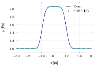
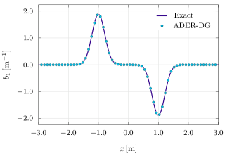
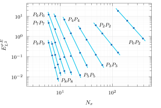
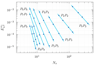
Figure 2: Numerical convergence results. In the top row, one-dimensional cuts (60 equidistant samples along the $x$ axis) of the pressure $p$ and the $x$ component of the interface field $b_{1}$ are presented at time $t=12\,\mathrm{s}$ (at the end of the second advection cycle), computed with a $\mathbb{P}_{9}\mathbb{P}_{9}$ ADER-DG scheme on a uniform grid of $6^{2}$ elements. In the bottom row we show logarithmic least-squares regression lines of the $L^{2}$ error norms of total energy density $\rho\,E$ and of the liquid volume fraction $\alpha_{1}$ for the ADER-DG $\mathbb{P}_{N}\mathbb{P}_{N}$ schemes of orders 3 to 10 and for the third order $\mathbb{P}_{0}\mathbb{P}_{2}$ ADER-WENO Finite Volume scheme.

Table 1: Numerical convergence results regarding the ADER-DG $\mathbb{P}_{N}\mathbb{P}_{N}$ schemes of nominal orders of accuracy 3 to 10 and the ADER-WENO $\mathbb{P}_{0}\mathbb{P}_{2}$ Finite Volume scheme for all conserved variables. The values reported in the Table are computed from a logarithmic least-square fit of the $L^{2}$ error norms as shown in Figures 2.

		$\alpha_{1}\,\rho_{1}$	$\alpha_{2}\,\rho_{2}$	$\rho\,u$	$\rho\,v$	$\rho\,E$	$\alpha_{1}$	$b_{1}$	$b_{2}$
$\mathbb{P}_{0}\mathbb{P}_{2}$	$\mathcal{O}_{L^{1}}$	2.9	3.1	2.9	2.9	2.9	2.9	2.8	2.8
	$\mathcal{O}_{L^{2}}$	2.9	3.0	2.9	2.9	2.9	2.9	2.8	2.8
	$\mathcal{O}_{L^{\infty}}$	2.8	3.0	2.8	2.8	2.8	2.8	2.7	2.7
$\mathbb{P}_{2}\mathbb{P}_{2}$	$\mathcal{O}_{L^{1}}$	3.2	3.2	3.2	3.2	3.2	3.2	3.2	3.2
	$\mathcal{O}_{L^{2}}$	3.2	3.2	3.2	3.2	3.2	3.2	3.2	3.2
	$\mathcal{O}_{L^{\infty}}$	3.1	3.1	3.1	3.1	3.1	3.1	3.1	3.1
$\mathbb{P}_{3}\mathbb{P}_{3}$	$\mathcal{O}_{L^{1}}$	4.3	4.3	4.3	4.3	4.3	4.3	4.3	4.3
	$\mathcal{O}_{L^{2}}$	4.3	4.3	4.3	4.3	4.3	4.2	4.3	4.3
	$\mathcal{O}_{L^{\infty}}$	4.2	4.1	4.2	4.2	4.2	4.2	4.3	4.3
$\mathbb{P}_{4}\mathbb{P}_{4}$	$\mathcal{O}_{L^{1}}$	5.5	6.1	5.5	5.5	5.5	5.5	5.5	5.5
	$\mathcal{O}_{L^{2}}$	5.3	5.6	5.3	5.3	5.3	5.3	5.3	5.3
	$\mathcal{O}_{L^{\infty}}$	5.1	5.3	5.1	5.1	5.0	5.1	5.0	5.0
$\mathbb{P}_{5}\mathbb{P}_{5}$	$\mathcal{O}_{L^{1}}$	6.5	7.3	6.5	6.5	6.5	6.4	6.4	6.4
	$\mathcal{O}_{L^{2}}$	6.2	6.8	6.2	6.2	6.2	6.2	6.1	6.1
	$\mathcal{O}_{L^{\infty}}$	5.8	6.6	5.8	5.8	5.8	5.7	5.8	5.8
$\mathbb{P}_{6}\mathbb{P}_{6}$	$\mathcal{O}_{L^{1}}$	7.2	8.6	7.2	7.2	7.2	7.2	7.1	7.1
	$\mathcal{O}_{L^{2}}$	6.9	8.0	6.9	6.9	6.9	6.9	6.8	6.8
	$\mathcal{O}_{L^{\infty}}$	6.6	8.1	6.6	6.6	6.6	6.5	6.4	6.3
$\mathbb{P}_{7}\mathbb{P}_{7}$	$\mathcal{O}_{L^{1}}$	8.3	10.0	8.3	8.3	8.3	8.2	8.1	8.1
	$\mathcal{O}_{L^{2}}$	8.0	9.4	8.0	8.0	8.0	7.9	7.7	7.7
	$\mathcal{O}_{L^{\infty}}$	7.8	9.4	7.8	7.8	7.8	7.4	7.1	7.1
$\mathbb{P}_{8}\mathbb{P}_{8}$	$\mathcal{O}_{L^{1}}$	9.7	11.1	9.7	9.7	9.7	9.6	9.6	9.6
	$\mathcal{O}_{L^{2}}$	9.3	10.2	9.3	9.3	9.3	9.2	9.2	9.2
	$\mathcal{O}_{L^{\infty}}$	8.7	9.1	8.7	8.7	8.7	8.8	8.4	8.4
$\mathbb{P}_{9}\mathbb{P}_{9}$	$\mathcal{O}_{L^{1}}$	10.7	11.7	10.7	10.7	10.7	10.6	10.6	10.6
	$\mathcal{O}_{L^{2}}$	10.2	11.0	10.2	10.2	10.2	10.1	10.1	10.1
	$\mathcal{O}_{L^{\infty}}$	9.9	11.2	9.9	9.9	9.9	10.0	9.7	9.7

Table 2: Numerical convergence results regarding the ADER-DG $\mathbb{P}_{N}\mathbb{P}_{N}$ schemes of nominal orders of accuracy 3 to 10 and the ADER-WENO $\mathbb{P}_{0}\mathbb{P}_{2}$ Finite Volume scheme for the liquid volume fraction $\alpha_{1}$. With $N_{x}$ we indicate the number of cells in one row of the Cartesian computational grid.

	$N_{x}$	$E_{L^{1}}$	$E_{L^{2}}$	$E_{L^{\infty}}$	$\mathcal{O}_{L^{1}}$	$\mathcal{O}_{L^{2}}$	$\mathcal{O}_{L^{\infty}}$
$\mathbb{P}_{0}\mathbb{P}_{2}$	128	$4.32\!\times\!10^{-2}$	$1.81\!\times\!10^{-2}$	$1.42\!\times\!10^{-2}$	$-$	$-$	$-$
	192	$1.41\!\times\!10^{-2}$	$5.90\!\times\!10^{-3}$	$4.76\!\times\!10^{-3}$	$2.76$	$2.76$	$2.70$
	256	$6.10\!\times\!10^{-3}$	$2.57\!\times\!10^{-3}$	$2.08\!\times\!10^{-3}$	$2.92$	$2.89$	$2.87$
	384	$1.83\!\times\!10^{-3}$	$7.75\!\times\!10^{-4}$	$6.29\!\times\!10^{-4}$	$2.97$	$2.96$	$2.95$
$\mathbb{P}_{2}\mathbb{P}_{2}$	48	$7.91\!\times\!10^{-3}$	$3.49\!\times\!10^{-3}$	$3.24\!\times\!10^{-3}$	$-$	$-$	$-$
	64	$3.07\!\times\!10^{-3}$	$1.37\!\times\!10^{-3}$	$1.32\!\times\!10^{-3}$	$3.29$	$3.25$	$3.13$
	96	$8.47\!\times\!10^{-4}$	$3.79\!\times\!10^{-4}$	$3.77\!\times\!10^{-4}$	$3.17$	$3.17$	$3.09$
	128	$3.47\!\times\!10^{-4}$	$1.55\!\times\!10^{-4}$	$1.56\!\times\!10^{-4}$	$3.10$	$3.10$	$3.07$
$\mathbb{P}_{3}\mathbb{P}_{3}$	24	$5.50\!\times\!10^{-3}$	$2.40\!\times\!10^{-3}$	$2.35\!\times\!10^{-3}$	$-$	$-$	$-$
	32	$1.46\!\times\!10^{-3}$	$6.67\!\times\!10^{-4}$	$7.04\!\times\!10^{-4}$	$4.61$	$4.46$	$4.19$
	48	$2.62\!\times\!10^{-4}$	$1.20\!\times\!10^{-4}$	$1.27\!\times\!10^{-4}$	$4.24$	$4.23$	$4.22$
	64	$8.18\!\times\!10^{-5}$	$3.73\!\times\!10^{-5}$	$3.87\!\times\!10^{-5}$	$4.05$	$4.06$	$4.14$
$\mathbb{P}_{4}\mathbb{P}_{4}$	12	$1.76\!\times\!10^{-2}$	$6.60\!\times\!10^{-3}$	$5.52\!\times\!10^{-3}$	$-$	$-$	$-$
	16	$3.24\!\times\!10^{-3}$	$1.38\!\times\!10^{-3}$	$1.48\!\times\!10^{-3}$	$5.89$	$5.44$	$4.59$
	24	$3.29\!\times\!10^{-4}$	$1.50\!\times\!10^{-4}$	$1.71\!\times\!10^{-4}$	$5.64$	$5.48$	$5.32$
	32	$8.15\!\times\!10^{-5}$	$3.69\!\times\!10^{-5}$	$4.03\!\times\!10^{-5}$	$4.86$	$4.86$	$5.02$
$\mathbb{P}_{5}\mathbb{P}_{5}$	8	$2.87\!\times\!10^{-2}$	$9.66\!\times\!10^{-3}$	$6.66\!\times\!10^{-3}$	$-$	$-$	$-$
	12	$1.88\!\times\!10^{-3}$	$7.53\!\times\!10^{-4}$	$7.87\!\times\!10^{-4}$	$6.72$	$6.29$	$5.27$
	16	$2.35\!\times\!10^{-4}$	$1.03\!\times\!10^{-4}$	$1.32\!\times\!10^{-4}$	$7.23$	$6.91$	$6.20$
	24	$2.59\!\times\!10^{-5}$	$1.18\!\times\!10^{-5}$	$1.36\!\times\!10^{-5}$	$5.43$	$5.36$	$5.62$
$\mathbb{P}_{6}\mathbb{P}_{6}$	6	$3.62\!\times\!10^{-2}$	$1.16\!\times\!10^{-2}$	$8.98\!\times\!10^{-3}$	$-$	$-$	$-$
	8	$5.97\!\times\!10^{-3}$	$2.12\!\times\!10^{-3}$	$1.74\!\times\!10^{-3}$	$6.27$	$5.92$	$5.71$
	12	$2.26\!\times\!10^{-4}$	$9.10\!\times\!10^{-5}$	$1.07\!\times\!10^{-4}$	$8.07$	$7.76$	$6.88$
	16	$3.65\!\times\!10^{-5}$	$1.62\!\times\!10^{-5}$	$1.62\!\times\!10^{-5}$	$6.34$	$6.00$	$6.55$
$\mathbb{P}_{7}\mathbb{P}_{7}$	6	$1.24\!\times\!10^{-2}$	$4.23\!\times\!10^{-3}$	$3.48\!\times\!10^{-3}$	$-$	$-$	$-$
	8	$1.17\!\times\!10^{-3}$	$4.64\!\times\!10^{-4}$	$5.41\!\times\!10^{-4}$	$8.19$	$7.68$	$6.47$
	10	$1.69\!\times\!10^{-4}$	$7.24\!\times\!10^{-5}$	$1.01\!\times\!10^{-4}$	$8.69$	$8.33$	$7.54$
	12	$4.22\!\times\!10^{-5}$	$1.87\!\times\!10^{-5}$	$2.07\!\times\!10^{-5}$	$7.60$	$7.41$	$8.68$
$\mathbb{P}_{8}\mathbb{P}_{8}$	7	$9.88\!\times\!10^{-4}$	$4.01\!\times\!10^{-4}$	$4.32\!\times\!10^{-4}$	$-$	$-$	$-$
	8	$2.69\!\times\!10^{-4}$	$1.17\!\times\!10^{-4}$	$1.42\!\times\!10^{-4}$	$9.73$	$9.23$	$8.35$
	9	$8.71\!\times\!10^{-5}$	$3.91\!\times\!10^{-5}$	$5.80\!\times\!10^{-5}$	$9.59$	$9.31$	$7.60$
	10	$3.20\!\times\!10^{-5}$	$1.49\!\times\!10^{-5}$	$1.79\!\times\!10^{-5}$	$9.50$	$9.17$	$11.16$
$\mathbb{P}_{9}\mathbb{P}_{9}$	6	$1.19\!\times\!10^{-3}$	$4.55\!\times\!10^{-4}$	$5.21\!\times\!10^{-4}$	$-$	$-$	$-$
	7	$2.53\!\times\!10^{-4}$	$1.10\!\times\!10^{-4}$	$1.49\!\times\!10^{-4}$	$10.02$	$9.24$	$8.13$
	8	$5.97\!\times\!10^{-5}$	$2.72\!\times\!10^{-5}$	$3.86\!\times\!10^{-5}$	$10.83$	$10.43$	$10.11$
	9	$1.62\!\times\!10^{-5}$	$7.59\!\times\!10^{-6}$	$9.05\!\times\!10^{-6}$	$11.07$	$10.84$	$12.31$

4.1.1 Problem setup

The initial condition for the liquid volume fraction $\alpha_{1}$ is given according to the chosen colour function profile, but bounding it between the two values $\alpha_{\mathrm{min}}=0.01$ and $\alpha_{\mathrm{max}}=0.99$, so that we have

$$\alpha_{1}(r)=\alpha_{\mathrm{min}}+\frac{\alpha_{\mathrm{max}}-\alpha_{\mathrm{min}}}{2}\,\operatorname{erfc}\left(\frac{r_{\ast}^{\prime}-1}{k_{\epsilon}}\right).\\$$ (78)

Since also the density fields should be transported with uniform velocity regardless of their value, we decided not to impose a constant value for $\rho_{1}$ and $\rho_{2}$, but rather specify a more interesting periodic two-dimensional wave configuration in the form

$$\rho_{1}(x,\ y)=\overline{\rho_{1}}+\delta\,\overline{\rho_{1}}\,\sin{\left[\omega\,(2\,x+y)\right]}\,\cos{\left[\omega\,(x-2\,y)\right]},$$ (79)

$$\rho_{2}(x,\ y)=\overline{\rho_{2}}+\delta\,\overline{\rho_{2}}\,\sin{\left[\omega\,(x-2\,y)\right]}\,\cos{\left[\omega\,(2\,x+y)\right]}.$$ (80)

The numerical values for the test are $u_{0}=v_{0}=3\,\mathrm{m\,s^{-1}}$, $R=1\,\mathrm{m}$, $k_{\epsilon}=0.3$, $\sigma=1\,\mathrm{N\,m^{-1}}$, $p_{\mathrm{atm}}=1\,\mathrm{Pa}$, $\overline{\rho_{1}}=1000\,\mathrm{kg\,m^{-3}}$, $\overline{\rho_{2}}=1\,\mathrm{kg\,m^{-3}}$, $\delta=0.1$, $\omega=\pi/3\,\mathrm{m^{-1}}$, $\Pi_{1}=20\,\mathrm{Pa}$, $\Pi_{2}=0\,\mathrm{Pa}$, $\gamma_{1}=4$, $\gamma_{2}=1.4$.

The computational domain is the square $\Omega=[-3\,\mathrm{m},\ 3\,\mathrm{m}]\times[-3\,\mathrm{m},\ 3\,\mathrm{m}]$ so that at $t=12\,\mathrm{s}$ we expect the water column to have completed two full advection cycles. We evolve the system from time $t=0$ to time $t=12\,\mathrm{s}$ for all $\mathbb{P}_{N}\mathbb{P}_{N}$, $N=2,\ 3,\ \ldots,\ 9$ schemes with local space-time DG predictor step performed in the primitive variable variant, using the HLL flux. The employed mathematical model is the nonconservative hyperbolic Godunov–Powell formulation. The results confirm that the error norms of the conserved variables decrease at a rate that is in agreement with the nominal order of accuracy of the scheme, and are summarised in Tables 1 and 2. In Table 2, we report the error norms and convergence rates for the liquid volume fraction $\alpha_{1}$, for numerical schemes of order up to 10. In Table 1, numerical details concerning the regression lines of the $L_{2}$ norms of the error for all variables are given. Since the interface field $\bm{\mathrm{b}}$ is evolved as a vector of independent state variables, as opposed standard schemes which differentiate the colour function and thus lose one order of accuracy for the discrete gradient, in our scheme the nominal high order convergence rate is achieved for the gradient field $\mathbf{b}$ as well. The regression lines for the mixture energy density $\rho\,E$ and for the liquid volume fraction $\alpha_{1}$ are plotted in Figure 2, where also one-dimensional cuts through the numerical solution are shown along the $x$ axis, comparing the exact solution derived in Section 2.4 with 60 uniformly spaced samples from a computation employing the $\mathbb{P}_{9}\mathbb{P}_{9}$ ADER-DG scheme on a very coarse uniform Cartesian grid composed of only $6^{2}$ total elements.

4.2 Interaction between a shock wave and a water column

With this test case we want to show that the ADER-DG schemes with a posteriori  subcell Finite Volume limiter are capable of computing solutions of nonconservative hyperbolic systems not only in smooth regions, but can also robustly deal with shock waves while preserving the sharp profile that characterises these flow features. Specifically, we want to reproduce the results of the experiment of Igra and Takayama [86], as it was done in [141].

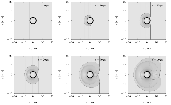
Figure 3: Numerical schlieren images of the early stages of the shock–water column interaction problem computed with a $\mathbb{P}_{3}\mathbb{P}_{3}$ ADER-DG scheme and a $\mathrm{TVD}$ subcell limiter on a mesh of spacing $\Delta x=\Delta y=0.0625\,\mathrm{mm}$.

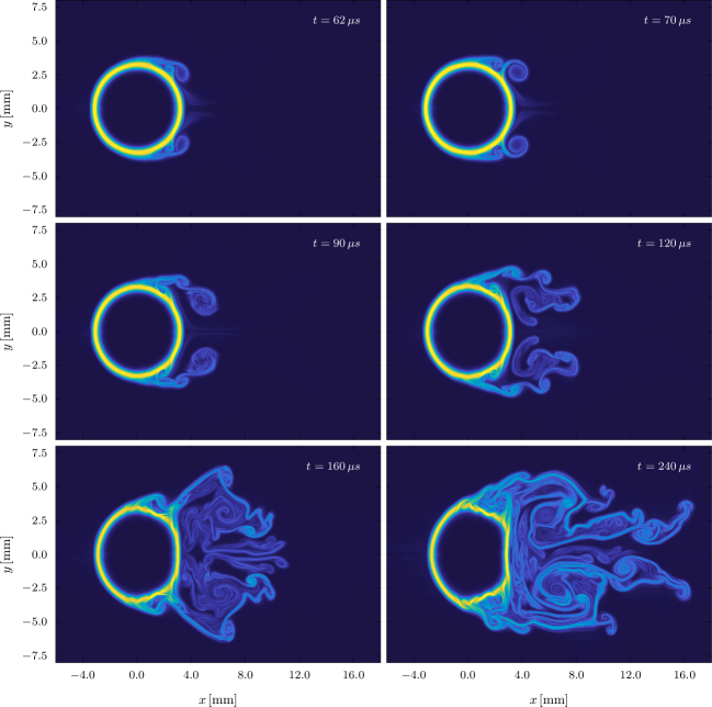
Figure 4: Visualisation of the interface transport by means of the filled contour plot of ${\sigma\,\lVert\bm{\mathrm{b}}\rVert}^{1/4}$ for the shock–water column interaction problem. The solution has been obtained with a $\mathbb{P}_{3}\mathbb{P}_{3}$ ADER-DG scheme and a $\mathrm{TVD}$ subcell limiter on a uniform mesh of spacing $\Delta x=\Delta y=0.0625\,\mathrm{mm}$.

The simulation setup is as follows: a cylindrical water column of radius $R=3.2\,\mathrm{mm}$ is initialised at the origin of the computational domain following the exact solution given in Section 2.4. The interface thickness parameter is $k_{\epsilon}=1/20$ and the surface tension coefficient is that of water, i.e. $\sigma=0.072\,\mathrm{N\,m^{-1}}$. Outside the water column, the pressure is set to $p=p_{\mathrm{atm}}=10^{5}\,\mathrm{Pa}$ and the liquid volume fraction is $\alpha_{1}=10^{-5}$, while inside the droplet we have $\alpha_{1}=1-10^{-5}$. The density for water and air are taken as $\rho_{1}=998.2\,\mathrm{kg\,m^{-3}}$ and $\rho_{2}=1.18\,\mathrm{kg\,m^{-3}}$, respectively. The parameters for the equation of state are the usual ideal gas parameters for air $\Pi_{2}=0\,\mathrm{Pa}$ and $\gamma_{2}=1.4$, while for the water we wanted to reproduce the correct speed of sound in the pure liquid phase so we set $\Pi_{1}=4.7\!\times\!10^{8}\,\mathrm{Pa}$ and $\gamma_{1}=4.7$. Since a perfectly pure phase is never present in our test, the speed of sound in water is slightly smaller than the correct one, but still significantly larger than the speed of sound in air, where the correct speed of sound is very well reproduced for $\alpha_{1}=10^{-5}$. A shock moving at speed $S_{\mathrm{s}}=1.3\,a_{\mathrm{air}}$ in the $x$ direction ($a_{\mathrm{air}}$ being the speed of sound in air, that is, we have a Mach 1.3 shock), with post-shock state computed following the jump relations found in [138], is localised, at time $t=-1.0\,\mu\mathrm{s}$, when the simulation is started, at a distance $\delta=S_{\mathrm{s}}\,\mathrm{m\,s^{-1}}\cdot\,1.0\,\mu\mathrm{s}$ (rounded to the nearest element edge) from the nominal edge of the droplet (see Figure 3 for a snapshot at time $t=0\,\mu\mathrm{s}$). A result of this sharp initialization of the shock profile can be clearly observed in the numerical schlieren images of Figure 3, in that two acoustic waves due to the startup error can be seen travelling upstream in the post-shock region.

In order to produce the results discussed in this section, we ran, for convenience, two distinct simulations with different domain sizes, but with the same mesh spacing. One simulation deals with the early phase of the simulation, that is the impact between the shock and the water column and the computational domain is the square $[-20\,\mathrm{mm},\ 20\,\mathrm{mm}]\times[-20\,\mathrm{mm},\ 20\,\mathrm{mm}]$, while for the simulation on longer timescales we adopt a rectangular domain $[-10\,\mathrm{mm},\ 30\,\mathrm{mm}]\times[-10\,\mathrm{mm},\ 10\,\mathrm{mm}]$. For the solution we employ a fourth order ADER-DG $\mathbb{P}_{3}\mathbb{P}_{3}$ scheme with primitive variable predictor step, supplemented with a robust second order TVD limiter with primitive variable reconstruction. The element size is the same for both simulations, since we use a grid of $640\times 640$ cells in the former case, and of $320\times 640$ cells in the latter. The numerical fluxes are computed with the HLL approximate Riemann solver.

In order to visualise the flow field, we plot the commonly used numerical schlieren pictures for the early stages of the simulation to highlight the shockwaves and aid comparison with the literature [141, 86], while, for the later stages of the simulation, we employ the key variable of the model, that would be the interface field $\bm{\mathrm{b}}$, to construct images that are very rich in detail and show quite effectively the complex turbulent structures which develop in this test problem, in a manner that is reminiscent of numerical schlieren pictures, since these are also nonlinearly scaled plots of the magnitude of a gradient.

In Figure 3. one can see the first time instants of the numerical experiment: discontinuities are very sharp, travel with the correct speed and in general show good agreement with both the experimental data of [86] and the simulations of [141]. It is then notable that at time $t=0\,\mu\mathrm{s}$ some interaction can be observed between the shock and the smoothing region of the water column, which extends symmetrically towards the centre of the water column and towards the environment past the nominal edge.

In Figures 4, at time $t=62\,\mathrm{ms}$ we can see the first vortical structures developing around the water column and, at time $t=120\,\mu\mathrm{s}$, Kelvin–Helmoltz-type [149, 82] instabilities are clearly distinguishable, while at time $t=240\,\mu\mathrm{s}$ one can also observe the presence of Richtmyer–Meshkov-type instabilities [131, 104].

With this visualization method, the process of formation of filaments in the edge of the water column, which then are drawn into the vortical flows in the wake of the obstacle, is quite apparent.

4.3 Droplet transport in two and three space dimensions

In this section, we conduct a systematic study of the stability and accuracy of the two new strongly hyperbolic systems of governing equations that have been proposed in this paper, which are both different from the original weakly hyperbolic model introduced in Schmidmayer et al  [141] . First, we set up a two-dimensional droplet in equilibrium, as prescribed by the exact solution given in Section 2.4, in a uniform velocity field with periodic boundary conditions, and track the time evolution of the domain-averaged curl constraint violations. The problem is analogous as the one used for the convergence study and is chosen because an exact solution for the problem is available, which allows to assess the correctness of the results unequivocally. Differently from what has been done in the convergence study, the sinusoidal density field given in Eq. (79), is replaced with two constant density values with ratio $\rho_{1}/\rho_{2}=1000$. In two space dimensions, the same test is repeated for the original weakly hyperbolic model of Schmidmayer et al  [141] , for the new hyperbolic formulation using the Godunov–Powell-type nonconservative products (denoted by GPNCP in the plots), and for another three runs with the new augmented hyperbolic GLM curl-cleaning system, with increasing values of the cleaning speed $c_{h}$, namely choosing $c_{h}\in\{10,\ 20,\ 40\}\,\mathrm{m\,s^{-1}}$. For each one of these five choices, we let the computations run up to a final time $t_{\mathrm{end}}=20.0\,\mathrm{ms}$, which corresponds to 20 full advection cycles, first on a coarse mesh of $16^{2}$ cells, and then on a finer grid counting $32^{2}$ elements, with the ADER-DG $\mathbb{P}_{5}\mathbb{P}_{5}$ scheme with ADER-WENO $\mathbb{P}_{0}\mathbb{P}_{2}$ a posteriori subcell limiter. The purpose of these runs is to verify how the different formulations react to mesh refinement and how they compare for a given resolution.

Then we carry out another set of five runs, studying the advection of a three-dimensional droplet with the ADER-DG $\mathbb{P}_{3}\mathbb{P}_{3}$ scheme with ADER-WENO $\mathbb{P}_{0}\mathbb{P}_{2}$ a posteriori subcell limiter, on a coarse mesh of $16^{3}$ elements, to extend the previous two-dimensional results to the full three-dimensional case.

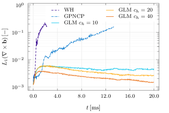
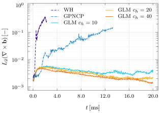
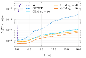
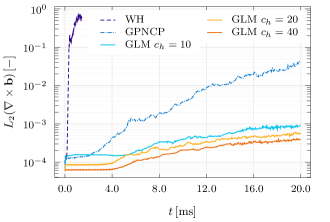
Figure 5: Time evolution of the $L_{1}$ and $L_{2}$ norms of the curl constraint violations for the two-dimensional droplet advection problem. In the top row, the results from a $\mathbb{P}_{5}\mathbb{P}_{5}$ ADER-DG scheme with ADER-WENO $\mathbb{P}_{0}\mathbb{P}_{2}$ subcell limiter on a uniform coarse grid composed of $16^{2}$ elements; in the bottom row, the results from the same method, but on a finer mesh composed of $32^{2}$ cells. In both cases, it is verified that curl errors are significantly reduced with the new GLM curl cleaning, with respect to those generated with the nonconservative Godunov–Powell-type formulation of the equations (GPNCP). In the GLM formulation, the constraint violations decrease with increasing cleaning speed $c_{h}$, as expected. Furthermore, on the coarser grid, the computation with the Godunov–Powell formulation fails after about 13 advection cycles ($13\,\mathrm{ms}$). In no case stable results can be obtained from the original weakly hyperbolic model.

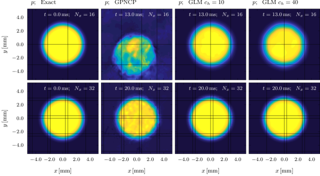
Figure 6: Numerical results for the two-dimensional droplet advection test problem. In the first row, we compare the results of the nonconservative Godunov–Powell model and of the augmented GLM curl cleaning system with two different values of cleaning speed $c_{h}$ with the exact solution. The snapshots of the pressure field are taken at time $t=13.0\,\mathrm{ms}$, which corresponds to thirteen advection cycles. The scheme used is ADER-DG $\mathbb{P}_{5}\mathbb{P}_{5}$ with ADER-WENO $\mathbb{P}_{0}\mathbb{P}_{2}$ subcell limiter and the mesh is composed of $16^{2}$ square control volumes. In the second row, the same comparison is carried out again, but on a finer mesh of $32^{2}$ elements at time $t=20.0\,\mathrm{ms}$, or after 20 advection cycles. The results from the nonconservative model show a significant deviation from the exact solution of the problem, while the GLM curl cleaning approach yields very stable and accurate results: on the coarser mesh, some numerical diffusion is visible by comparing with the exact solution, but on the finer mesh numerical diffusion can be considered negligible.

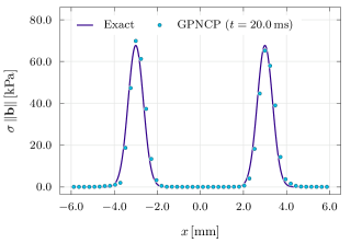
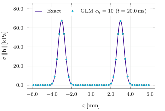
Figure 7: One-dimensional cuts (50 uniform samples along the $x$ axis) of the interface energy $\sigma\,\lVert\bm{\mathrm{b}}\rVert$ for the two-dimensional droplet advection test problem. The cuts are taken at time $t=20.0\,\mathrm{ms}$ (after 20 advection cycles) The scheme used is ADER-DG $\mathbb{P}_{5}\mathbb{P}_{5}$ with ADER-WENO $\mathbb{P}_{0}\mathbb{P}_{2}$ subcell limiter and the mesh is composed of $32^{2}$ square control volumes.

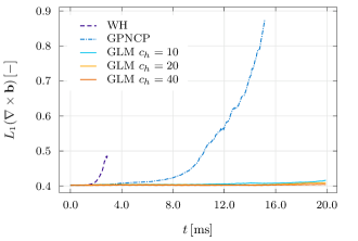
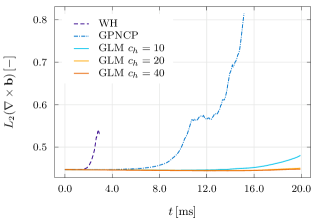
Figure 8: Time evolution of the $L_{1}$ and $L_{2}$ norms of the curl constraint violation for the three-dimensional droplet advection problem. The results obtained for the two-dimensional experiments are confirmed. It is quite apparent that, employing the GLM curl cleaning, the constraint violation grows much slower than with the Godunov–Powell-type formulation of the system (GPNCP). In particular, in this latter case the computation fails after about 15 advection cycles ($15.0\,\mathrm{ms}$), while the augmented GLM curl cleaning system shows much better stability properties. The simulations have been carried out using a $\mathbb{P}_{3}\mathbb{P}_{3}$ ADER-DG scheme with ADER-WENO $\mathbb{P}_{0}\mathbb{P}_{2}$ subcell limiter on a uniform grid composed of $16^{3}$ elements.

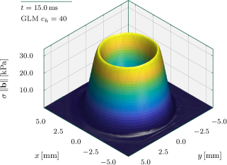
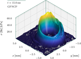
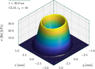
Figure 9: Two-dimensional slices, at $z=0$, of the solution for the surface energy $\sigma\,\lVert\bm{\mathrm{b}}\rVert$, for the three-dimensional droplet advection test. The top left panel shows the exact solution of the problem. The top right plot is the numerical solution at time $t=15.0\,\mathrm{ms}$, that is, after fifteen advection cycles, obtained using the GLM curl cleaning formulation of the model with cleaning speed $c_{h}=40$, showing good agreement with the exact solution. The bottom left plot represents the solution at $t=15.0\,\mathrm{ms}$ obtained with the Godunov–Powell nonconservative formulation of the model (GPNCP); strong artefacts are visible. The bottom right plot shows the GLM curl cleaning solution after five additional advection cycles, with comparatively minor deformation of the interface. The results are obtained with a fourth order ADER-DG $\mathbb{P}_{3}\mathbb{P}_{3}$ and ADER-WENO $\mathbb{P}_{0}\mathbb{P}_{2}$ subcell limiter, on a very coarse mesh of $16^{3}$ elements.

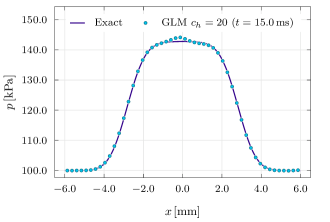
Figure 10: One-dimensional cuts (50 uniform samples along the $x$ axis), at $z=y=0$, of the solution for the pressure field $p$, for the three-dimensional droplet advection problem. On the left, the solution obtained with the Godunov–Powell nonconservative formulation of the model (GPNCP). On the right, the solution from the GLM curl cleaning formulation, with cleaning speed $c_{h}=20$. One can note that, at time $t=15.0\,\mathrm{ms}$, after fifteen full advection cycles, the nonconservative formulation significantly deviates from the exact solution derived in Section 2.4, while the error is very well contained by the GLM curl cleaning. The results are obtained with a fourth order ADER-DG $\mathbb{P}_{3}\mathbb{P}_{3}$ and ADER-WENO $\mathbb{P}_{0}\mathbb{P}_{2}$ subcell limiter, on a very coarse mesh of $16^{3}$ elements.

The droplet has radius $R=3\,\mathrm{mm}$ and is centred at the origin of a square domain $\Omega=[-6\,\mathrm{mm},\ 6\,\mathrm{mm}]\times[-6\,\mathrm{mm},\ 6\,\mathrm{mm}]$, the liquid and gas density are respectively set to $\rho_{1}=1000\,\mathrm{kg\,m^{-1}}$ and $\rho_{2}=1\,\mathrm{kg\,m^{-1}}$ throughout the domain. The volume fraction follows Eq. (78), with $\alpha_{\mathrm{min}}=0.01$ and $\alpha_{\mathrm{max}}=0.99$, and the interface field is given by (33), with the dimensionless interface thickness parameter being $k_{\epsilon}=1/6$ for the two-dimensional tests and $k_{\epsilon}=1/3$ for the three-dimensional problem, additionally setting $b_{3}=0$ for the two-dimensional runs. The pressure is initialised following the exact solution (37), with atmospheric pressure $p_{\mathrm{atm}}=100\,\mathrm{kPa}$, and the uniform velocity field components are $u_{0}=12\,\mathrm{m\,s^{-1}}$, $v_{0}=12\,\mathrm{m\,s^{-1}}$, and $w_{0}=12\,\mathrm{m\,s^{-1}}$ in three space dimensions or $w_{0}=0\,\mathrm{m\,s^{-1}}$ in two dimensions. The parameters for the equation of state are $\Pi_{1}=1\,\mathrm{MPa}$, $\Pi_{2}=0$, $\gamma_{1}=4$, $\gamma_{2}=1.4$, and the surface tension coefficient is set to $\sigma=60\,\mathrm{N\,m^{-1}}$.

The results are depicted in Figures 5, 6, and 7. In Figure 5, we plot the time evolution of the normalised $L_{1}$ and $L_{2}$ norms of the curl constraint violations, defined as

$$\left.L_{1}(\nabla\times\bm{\mathrm{b}})\right.=\dfrac{\left.\displaystyle\int_{\Omega}\sqrt{\,{(\nabla\times\bm{\mathrm{b}})}^{\mathsf{T}}\,\nabla\times\bm{\mathrm{b}}\,}\right.}{\left.\displaystyle\int_{\Omega}\sqrt{\,\operatorname{tr}{\left[{(\nabla\bm{\mathrm{b}})}^{\mathsf{T}}\,\nabla\bm{\mathrm{b}}\right]\,}}\right|_{t=0}},\qquad\left.L_{2}(\nabla\times\bm{\mathrm{b}})\right.=\dfrac{\left.\displaystyle\int_{\Omega}{\left|\,{(\nabla\times\bm{\mathrm{b}})}^{\mathsf{T}}\,\nabla\times\bm{\mathrm{b}}\,\right|}\right.}{\left.\displaystyle\int_{\Omega}{\left|\,\operatorname{tr}{\left[{(\nabla\bm{\mathrm{b}})}^{\mathsf{T}}\,\nabla\bm{\mathrm{b}}\right]\,}\right|\,}\right|_{t=0}}.$$ (81)

We observe that in all cases the same trend is apparent: the curl error given by the weakly hyperbolic model quickly grows until the computation terminates with unphysical values at rather early times, while the new strongly hyperbolic variants of the governing equations are stable, at least with increasing mesh refinement. It seems that not much can be done to improve the stability of the weakly hyperbolic model, which in the run with finer mesh blows up even earlier than with the coarse grid, most likely due to the smaller numerical dissipation of the scheme. In the long term, it is always true that the curl errors are lower with GLM curl cleaning than they are with the nonconservative Godunov–Powell-type model. One can also see that the higher the cleaning speed $c_{h}$ is, the smaller the constraint violations are. Moreover, on the fine mesh, the nonconservative Godunov–Powell system, while still generating much larger errors than the augmented GLM model (clearly visible also in the pressure field shown in Figure 6), could be solved for the full 20 advection cycles, as opposed to only 13 on the coarse mesh.

Concerning the effects of numerical dissipation, we can see that the curl errors for the GLM curl cleaning simulations on the coarse grid decrease in time with the aid of numerical diffusion, which reduces the overall steepness of the interface field. This effect can be easily quantified by inspecting Figure 6 where it is apparent that with the coarse mesh the pressure field after thirteen advection cycles is more diffused than in the initial condition, while this effect is minimised by mesh refinement, as one can clearly see in Figure 7, where the profile of the interface field on the GLM simulations is still in perfect agreement with the exact solution after 20 full advection cycles. Regarding this simulation with the finer grid, the curl error timeseries no longer shows the effects of numerical dissipation and in the first stages of the computation (up to about three to four advection cycles) one can see that the curl errors are maintained at a very precise constant value, suggesting that a sort of balance is established between the sources of the curl errors in the numerical scheme and their transport via the Maxwell-type curl cleaning waves of the augmented GLM system. Also, one can note that, for the run with cleaning speed $c_{h}=40\,\mathrm{m\,s^{-1}}$, in this early phase, the curl error is kept very close to its non-zero initial value, which is given by the necessity of projecting the pressure profile on the piecewise-polynomial Discontinuous Galerkin data representation, even if evaluated at machine precision from an exact formula.

In the three-dimensional tests, the effects of numerical diffusion are not seen because the interface profile was chosen to be smoother than the one used for the two-dimensional simulations from the beginning. Otherwise, the same observations given for the two-dimensional case are valid, namely one can construct a hierarchy of the simulations based on the entity of the curl-constraint violations, that sees the weakly hyperbolic model break down very early, the Godunov–Powell-type symmetrisable model being more stable, but more sensitive in the long term than the GLM cleaning simulations, which in turn have lower errors for higher cleaning speeds. The timeseries of the constraint violations are plotted in Figure 8, where the error is kept essentially equal to the initial value with the GLM curl cleaning, while it grows rather quickly for the Godunov–Powell formulation, for which the computation stops after completing 15 advection cycles.

In Figure 9, we show a set of two-dimensional slices of the solution for the interface energy and we observe that, as for the analogous two-dimensional test, the hyperbolic Godunov–Powell model shows severe degradation of the interface field after fifteen advection cycles and the droplet is even shifted out of centre, as was the two-dimensional droplet in the second panel of Figure 6. At the same time instant, the GLM curl cleaning formulation seems to adequately match the exact solution, despite using a rather coarse mesh, and shows no spurious shift of the centre of mass of the droplet, as seen also in the one-dimensional cuts of Figure 10.

4.4 Oscillation of an elliptical water column

We continue our systematic comparison of the different formulations of the hyperbolic surface tension model under investigation with a test involving the oscillation of an elliptical water column, which, due to the elongated initial shape, is not in mechanical equilibrium and tends to deform towards restoring a circular shape. The phenomenon is of periodic nature since when the droplet has indeed reached a circular shape, it also stores an amount of kinetic energy such that it starts to elongate again perpendicularly with respect to the previous major axis, up to a maximum deformation, then deforming back to a circular shape and finally to the initial configuration.

4.4.1 Problem setup

For the description of the geometry of a smoothed elliptical water column having a nominal interface defined by the parametric equation ${\bm{\mathrm{r}}_{\mathrm{b}}=(x_{\mathrm{b}},\ y_{\mathrm{b}})=(R_{x}\,\cos\psi,\ R_{y}\,\sin\psi)}$,

we introduce the following coordinates: for each point $(x,\ y)$ in the Cartesian plane the local eccentric anomaly $\psi$ is defined implicitly by the formulas

$$\cos^{2}\psi(x,\ y)=\frac{R_{y}^{2}\,x^{2}}{R_{y}^{2}\,x^{2}+R_{x}^{2}\,y^{2}},\qquad\sin^{2}\psi(x,\ y)=\frac{R_{x}^{2}\,y^{2}}{R_{y}^{2}\,x^{2}+R_{x}^{2}\,y^{2}};$$ (82)

for each point $(x,\ y)$, we can then define the nominal radius of the ellipse in the direction of the local eccentric anomaly

$$R_{\psi}(\psi(x,\ y))=\sqrt{R_{x}^{2}\,\cos^{2}\psi+R_{y}^{2}\,\sin^{2}\psi},$$ (83)

which would be the length of the segment running from the centre of the water column (located at the origin of the reference system) to the intersection between the ellipse boundary and the line connecting said generic point with the origin. Then we denote as usual with $r(x,\ y)=\sqrt{{x}^{2}+{y}^{2}}$ the distance of a generic point from the centre of the water column. Then, given its dimensionless form $r_{\ast}$ with respect to $R_{\psi}$, the colour function $c$, its gradient $\bm{\mathrm{b}}=[b_{1},\ b_{2},\ 0]$ and the liquid volume fraction $\alpha_{1}$ are given as

$$c(x,\ y)=\frac{1}{2}\,\operatorname{erfc}{\left(\frac{r-R_{\psi}}{\epsilon}\right)},$$ (84)

$$\alpha_{1}(x,\ y)=\alpha_{\mathrm{min}}+(\alpha_{\mathrm{max}}-\alpha_{\mathrm{min}})\,c(x,\ y),$$ (85)

$$b_{1}(x,\ y)=-\frac{x}{\sqrt{\pi}\,\epsilon\,r}\,\exp{\left[-{\left(\frac{r-R_{\psi}}{\epsilon}\right)}^{2}\right]}\,\left[1-\left(1-\frac{R_{y}^{2}}{R_{x}^{2}}\right)\frac{R_{\psi}}{r}\,\sin^{2}\psi\right],$$ (86)

$$b_{2}(x,\ y)=-\frac{y}{\sqrt{\pi}\,\epsilon\,r}\,\exp{\left[-{\left(\frac{r-R_{\psi}}{\epsilon}\right)}^{2}\right]}\,\left[1-\left(1-\frac{R_{x}^{2}}{R_{y}^{2}}\right)\frac{R_{\psi}}{r}\,\cos^{2}\psi\right],$$ (87)

while the pressure field is initialised as a local application of the solution for a cylindrical water column in the form

$$p\left(r_{\ast}\right)=p_{\mathrm{atm}}+(d-1)\,\frac{\sigma}{R}\,\int_{r_{\ast}}^{\infty}\frac{1}{\sqrt{\pi}\,k_{\epsilon}\,r_{\ast}^{\prime}}\,\exp\left[-{\left(\frac{r_{\ast}^{\prime}-1}{k_{\epsilon}}\right)}^{2}\right]\,\operatorname{d\!}{r_{\ast}^{\prime}},$$ (88)

$$\quad\text{with}\quad r_{\ast}(x,\ y)=\frac{r(x,\ y)}{R_{\psi}(\psi(x,\ y))},\quad k_{\epsilon}=\dfrac{\epsilon}{R_{\kappa}},$$

where by local we mean that an average curvature radius $R_{\kappa}$, defined at each point $(x,\ y)$ inside, on the nominal boundary, or outside of the droplet, is computed by averaging the curvature along the nominal boundary of the ellipse, with a weight function inversely proportional to the square of the distance from the interface ${\left[R_{\psi}(\psi)-r(x,\ y)\right]}^{2}$, so that we have

$$R_{\kappa}(x,\ y)={\left\{\dfrac{\displaystyle\int_{0}^{2\,\pi}\dfrac{1}{{\left[R_{\psi}(\psi)-r(x,\ y)\right]}^{2}}\,\dfrac{R_{x}\,R_{y}}{R_{x}^{2}\,\sin^{2}\psi+R_{y}^{2}\,\cos^{2}\psi}\,\operatorname{d\!}{\psi}}{\displaystyle\int_{0}^{2\,\pi}\dfrac{1}{{\left[R_{\psi}(\psi)-r(x,\ y)\right]}^{2}}\,\sqrt{R_{x}^{2}\,\sin^{2}\psi+R_{y}^{2}\,\cos^{2}\psi}\,\operatorname{d\!}{\psi}}\right\}}^{-1}.$$ (89)

This averaging procedure yields a local curvature radius such that the initial pressure configuration is similar to the one occurring at oscillation extrema, i.e. at the end of every half-period, when the kinetic energy of the droplet is zero, as it is set initially. Even if based only on geometrical considerations, this initial condition is sufficient for individuating very clearly only the main oscillation mode of the droplet, allowing to obtain a clean estimate of the oscillation period. A comparison between the geometrically-derived initial pressure field and the configuration after three oscillation periods is shown in Figure 11, together with the complex flow features that are generated in the earliest instants of the simulation.

The density fields are set to the uniform values $\rho_{1}^{0}$ and $\rho_{2}^{0}$ throughout the computational domain, as is the velocity field for which we set $\bm{\mathrm{u}}={[0,\ 0,\ 0]}^{\mathsf{T}}$. The numerical values employed for this test problem are: $\rho_{1}^{0}=1000\,\mathrm{kg\,m^{-3}}$, $\rho_{2}^{0}=1\,\mathrm{kg\,m^{-3}}$, $p_{\mathrm{atm}}=100\,\mathrm{kPa}$, $R_{x}=3\,\mathrm{mm}$, $R_{y}=2\,\mathrm{mm}$, $\alpha_{\mathrm{min}}=0.01$, $\alpha_{\mathrm{max}}=0.99$, $\sigma=60\,\mathrm{N\,m^{-1}}$. The parameters for the stiffened gas equation of state are: $\Pi_{1}=1\,\mathrm{MPa}$, $\Pi_{2}=0$, $\gamma_{1}=4$, $\gamma_{2}=1.4$. The domain is the square $[-6\,\mathrm{mm},\ 6\,\mathrm{mm}]\times[-6\,\mathrm{mm},\ 6\,\mathrm{mm}]$ and additionally, the initial condition is rotated counter-clockwise by 30 degrees, in order to avoid mesh alignment. In a first batch of tests, we set $\epsilon=0.5\,\mathrm{mm}$ and discretise the computational domain with $64^{2}$ square cells, then solving with an ADER-DG $\mathbb{P}_{5}\mathbb{P}_{5}$, ADER-WENO $\mathbb{P}_{0}\mathbb{P}_{2}$ Finite Volume limiter and HLL flux. These simulations are intended to test the capability of the proposed models in a dynamical setting where the interface deforms significantly under the effect of strong surface tension, and verify that the GLM curl cleaning approach can deal with the violations of involution constraints that such deformations generate.

In a second run, in order to study the sensitivity of results and in particular of the oscillation period to the thickness of the diffuse interface region, we set $\epsilon=0.25\,\mathrm{mm}$, impose no initial rotation of the droplet, thus aligning the two axis of the ellipse with the reference frame, and compute the solution of the problem on a uniform grid of $50^{2}$ elements, with an eight order ADER-DG $\mathbb{P}_{7}\mathbb{P}_{7}$ scheme, ADER-WENO $\mathbb{P}_{0}\mathbb{P}_{2}$ Finite Volume limiter, and Rusanov flux.

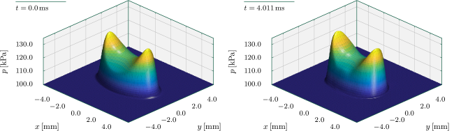
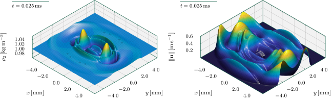
Figure 11: Initial stages of the elliptical droplet oscillation problem, In the top row, oscillation periods ($t=4.011\,\mathrm{ms}$). In the bottom row, density of the gas phase (on the left) and flow speed distribution (on the right) at time $t=0.025\,\mathrm{ms}$. The Godunov–Powell nonconservative formulation of the model was solved with a $\mathbb{P}_{7}\mathbb{P}_{7}$ ADER-DG scheme and ADER-WENO $\mathbb{P}_{0}\mathbb{P}_{2}$ subcell limiter on a uniform grid of $50^{2}$ elements.

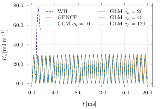
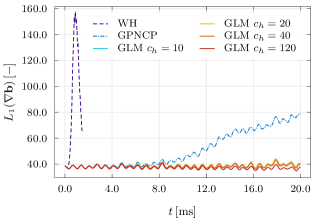
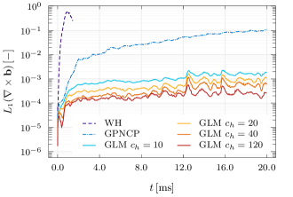
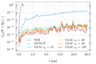
Figure 12: Time evolution of global dynamics and of curl errors for an oscillating elliptical water column. In the top row, left to right: the total kinetic energy $E_{\mathrm{k}}$ and the $L_{1}$ norm of $\nabla\bm{\mathrm{b}}$ over time. In the bottom row, the timeseries for the $L_{1}$ and $L_{2}$ norms of the curl constraint violation error. One can see that all the GLM curl cleaning simulation yield a constant oscillation period and kinetic energy is preserved quite well over more than $6\!\times\!10^{5}$ timestep, while the Godunov-Powell nonconservative formulation of the governing equations (GPNCP) shows signs of deterioration of the kinetic energy oscillation envelope. Moreover, curl errors decrease for increasing cleaning speed $c_{h}$, and in general GLM curl cleaning is effective in containing them, compared to the Godunov-Powell nonconservative formulation, and especially compared to the original weakly hyperbolic (WH) system, for which the computation fails rather early. The simulations employed a $\mathbb{P}_{5}\mathbb{P}_{5}$ ADER-DG scheme with ADER-WENO $\mathbb{P}_{0}\mathbb{P}_{2}$ subcell limiter on a uniform grid composed of $64^{2}$ elements.

4.4.2 Discussion of the results

In this test, the Discontinuous Galerkin scheme is supplemented by a third order ADER-WENO $\mathbb{P}_{0}\mathbb{P}_{2}$ Finite Volume subcell limiter, which is an important ingredient for obtaining accurate results in this test and for preserving the very complex smooth structures that arise in the flow (see Figure 11); in fact, even with the the extremely large value we adopted for $\sigma$, the timescales associated with the theoretical oscillation period $T_{\mathrm{p}}^{\mathrm{a}}$, given for small amplitude oscillations by the formula [146, 65]

$$T_{\mathrm{p}}^{\mathrm{a}}=2\,\pi\,{\left[\sqrt{\frac{6\,\sigma}{(\rho_{1}+\rho_{2})\,R^{3}}}\right]}^{-1},\quad\text{with}\quad R=\frac{R_{x}+R_{y}}{2},$$ (90)

are much larger than the timestep restriction for the numerical method in use and thus the task can be regarded as a long-time integration problem. Specifically, to test the robustness of the different formulations of the governing equations we evolved an oscillating elliptical droplet up to a final time $t_{\mathrm{end}}=20.0\,\mathrm{ms}$, which correspond to $605914$ timesteps for the GLM curl cleaning simulation with $c_{h}=10$, while the simulation with $c_{h}=120$ required $649578$ timesteps, and the Godunov–Powell simulation reaches the final time in $637368$ timesteps. During the run, the total kinetic energy of the droplet $E_{\mathrm{k}}$ is tracked and subsequently employed to measure the oscillation period of the droplet. Together with the kinetic energy, also the $L_{1}$ and $L_{2}$ norms of the curl errors and of the gradient of the interface field $\nabla\bm{\mathrm{b}}$ are computed and stored. The norms of $\nabla\bm{\mathrm{b}}$ can be taken as an indicator of the roughness of the solution, which, with reference to Figure 12, can in turn indicate that the solution is developing spurious artefacts instead of maintaining its interface field smooth; alternatively, since the interface field is sensitive to numerical diffusion, seeing that $\nabla\bm{\mathrm{b}}$ does not quickly decay, indicates that the scheme is not introducing excessive artificial dissipation into the system. The timeseries for these integral quantities are shown in Figure 12, and again it appears that the GLM curl cleaning approach yields the best results: the Godunov–Powell simulation show some signs of deterioration of the kinetic energy oscillation envelope and an increase in the average magnitude of the gradients of the interface field. On the other side, the timeseries of kinetic energy obtained with GLM curl cleaning does not show any signs of decay in the solution quality, and this is reflected in the fact that violations of curl involutions are significantly lower with respect to the Godunov–Powell run. Moreover, after fifteen oscillation periods, we cannot observe any decay in kinetic energy due to numerical diffusion, which one would expect from lower order explicit methods for compressible flow. Finally, it can be confirmed that the weakly hyperbolic formulation of the equations is not well suited for solving time-dependent problems with high order Godunov-type schemes, as our computations, employing a sixth order ADER-DG method on $64^{2}$ cells, blew up before a single full oscillation period could be simulated.

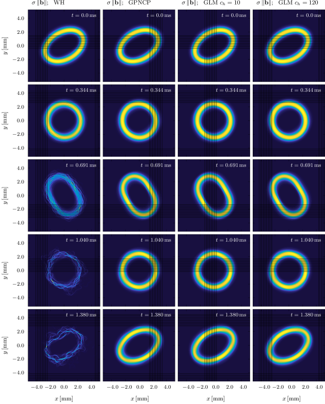
Figure 13: Early stages of the oscillation of a two-dimensional elliptical droplet. The first column shows the quick deterioration of the interface field that is observed when solving the weakly hyperbolic formulation of the model (WH), the second shows that restoring hyperbolicity with the Godunov-Powell–type nonconservative products (GPNCP) prevents such ill behaviour, and the same is true for the GLM curl cleaning approach with different cleaning speeds $c_{h}$.

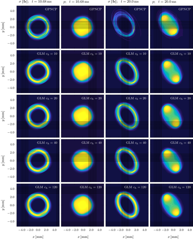
Figure 14: Late stages of the oscillation of a two-dimensional elliptical droplet. In the first two columns we plot the surface energy $\sigma\,\lVert\bm{\mathrm{b}}\rVert$ and the pressure $p$ three quarters through the eighth oscillation cycle, and in the last two at about half of the fifteenth oscillation. The first row shows the results of the nonconservative Godunov–Powell-type model, with clear signs of deterioration of the solution, while in the other rows one can see the consistent results of GLM curl cleaning with several cleaning speeds $c_{h}$.

In Figure 13, we see that the simulation reproduces the expected global dynamic behaviour in that the droplet can be observed achieving a circular shape at a quarter and at three quarters of the oscillation period, when the maxima of kinetic energy are reached, while the minima of kinetic energy, defining the half-period and end-period times, correspond to the maximum elongation of the droplet in orthogonal directions. In these early stages of the simulation, we can observe very little difference between the results from the GLM curl cleaning simulations with low cleaning speed ($c_{h}=10\,\mathrm{m\,s^{-1}}$) or high cleaning speed ($c_{h}=120\,\mathrm{m\,s^{-1}}$), as well as with respect to the solutions of the Godunov–Powell nonconservative variant of the model. On the contrary, it is clear in the first column of Figure 13, that the original weakly hyperbolic model does instead develop spurious filaments in the interface field starting from the first oscillation period, leading to a very early breakdown of the computation.

In Figure 14, we compare the solutions, at two different time instants, obtained from the Godunov–Powell-type formulation of the model (16) and from the augmented GLM curl cleaning system (26), with several different values of cleaning speed $c_{h}$. At both time instants, we can see only small differences among the simulations using GLM curl cleaning, while it is clear in the first column of Figure 13 that with the nonconservative Godunov–Powell-type model some secondary subdivisions of the interface field are starting to develop at time $t=10.68\,\mathrm{ms}$, three quarters through the eighth oscillation cycle. The effects on the pressure field are not yet visible at this stage, but one can see in the last two columns of Figure 14 that at the end time $t=20\,\mathrm{ms}$, about half of the fifteenth oscillation cycle, these artefacts have further developed and have caused not only a visible distortion of the pressure field, but also determined a bulk shift of the full droplet, which is no longer centred at the origin of the computational domain, as already seen in the three-dimensional droplet in Figures 9 and Figure 10.

Our numerical estimate of the oscillation period is obtained by solving the nonconservative Godunov–Powell-type formulation of the model with an ADER-DG $\mathbb{P}_{7}\mathbb{P}_{7}$ scheme and ADER-WENO $\mathbb{P}_{0}\mathbb{P}_{2}$ subcell limiter on a mesh of $50^{2}$ cells; the interface thickness is set to $\epsilon=2.5\times 10^{-4}$. The deviation of the numerical estimate $T_{\mathrm{p}}=1.337\,\mathrm{ms}$ with respect to the analytical prediction of $T_{\mathrm{p}}^{\mathrm{a}}=1.3097\,\mathrm{ms}$ is of $2.1\%$. While not exact, the result can be considered satisfactory, since the difference can be attributed in part to the fact that the reference formula (90) was obtained under the assumption of small amplitude oscillations, and is thus valid only for almost circular droplets. Another potential source of deviation from the predictions of linear theory is the diffuse interface representation of the droplet, which distributes mass differently with respect to the ideal sharp interface jump. In this regard, we computed the oscillation period also from another set of simulations, namely those comparing the long-term behaviour of the Godunov–Powell and of the GLM curl cleaning formulations of the model, employing an ADER-DG $\mathbb{P}_{5}\mathbb{P}_{5}$ scheme and ADER-WENO $\mathbb{P}_{0}\mathbb{P}_{2}$ subcell limiter on a mesh of $64^{2}$ elements, while the interface thickness is doubled with respect to the previous run from $\epsilon=2.5\times 10^{-4}$ to $\epsilon=5.0\times 10^{-4}$. The estimated period for this more diffuse droplet is $T_{\mathrm{p}}^{\textsc{gpncp}}=1.375\,\mathrm{ms}$ with the Godunov–Powell-type variant of the model, while we computed $T_{\mathrm{p}}^{\textsc{glm}}=1.377\,\mathrm{ms}$ with the GLM curl cleaning formulation. These estimates for the droplet with a thicker interface correspond to a difference of $2.8\%$ to $3.0\%$ with respect to the previous estimate $T_{\mathrm{p}}=1.337\,\mathrm{ms}$, and deviate by $5.0\%$ to $5.1\%$ from the small oscillations theory, despite the interface thickness being twice as large as the one used in the previous run.

5 Summary and conclusions

In this paper, we have presented two new strongly hyperbolic reformulations of the originally weakly hyperbolic two-phase flow model with surface tension [17, 141]. Both reformulations heavily rely on the curl-free constraint (7) of the interface vector field $\bm{\mathrm{b}}$. The first of the two hyperbolic extensions was based on the theory of Symmetric Hyperbolic and Thermodynamically Compatible (SHTC) systems [71, 76, 119], and consists in modifying the momentum and energy equations by adding some symmetrising nonconservative terms, which are multiples of the curl involution constraint (7) and thus, are formally zeros. The second reformulation of model [141] was based on ideas developed in the context of numerical Magnetohydrodynamics (MHD) and is more specifically based on the hyperbolic Generalized Lagrangian Multiplier (GLM) divergence-cleaning approach of Munz et al  [108, 34].

We have then carefully compared the stability of the two reformulations, their accuracy, and consistency properties as well as showing the behaviour of the original weakly hyperbolic model. The comparison seems to suggest that the weakly hyperbolic formulation is not suitable for a direct discretisation with general purpose explicit high order schemes, such as the ADER Discontinuous Galerkin and ADER Finite Volume methods of this work, whereas the novel strongly hyperbolic reformulations can be shown to produce correct results, specifically for simulating the dynamics of oscillating droplets and they in general yield numerical results that are in agreement with analytical predictions.

Of the two proposed models, the GLM approach uses hyperbolic constraint cleaning in order to minimise the violations of the curl involution constraint, obtaining a strongly hyperbolic and conservative model, while the first differs substantially from the weakly hyperbolic system [17, 141] in that it has a full set of eigenvectors, but no explicit enforcement of curl involution constraints has been introduced. The results obtained with the GLM curl cleaning formulation are measurably better than those of the first hyperbolic model here proposed, and this suggests that it is important to enforce such constraints in order to achieve reliable results in long time integration problems. In any case, it can be noted that for short times, or by increasing the resolution of the spatial discretisation, the nonconservative Godunov–Powell model can yield solutions that are comparable to those obtained using GLM curl cleaning (see for example Figures 13 and 7). This is not the case for the weakly hyperbolic model, which does not seem to improve its behaviour significantly with mesh refinement, as apparent in Figure 5

Another finding, that is completely independent of the model variant or of the numerical scheme in use, being based on an exact solution common to all three variants in consideration, is that the pressure jump between the environment and region inside of a droplet is not particularly sensitive to the thickness of the smoothed interface, and in particular the error vanishes quadratically with respect to the width of the smoothing region. This is also reflected in the bulk dynamical behaviour of oscillating droplets, in the sense that the oscillation period can be predicted with sufficient accuracy even with smoothed interfaces.

Future developments will concern the extension of the mathematical model of this paper to the conservative multi-phase model of [134, 133] with pressure and velocity relaxation, as well as the development of exactly curl preserving schemes on suitably staggered meshes, along the lines of exactly divergence-preserving schemes for the Maxwell and MHD equations [161, 36, 14, 9, 12], which need to be properly extended to curl-type involution constraints. We will also consider applications of the hyperbolic GLM curl cleaning approach to the first order hyperbolic reformulation of the nonlinear Schrödinger equation recently proposed in [37].

References

- [1] R. Abgrall and S. Karni. Computations of compressible multifluids. Journal of Computational Physics, 169(2):594–623, 2001.
- [2] D.M. Anderson, G.B. McFadden, and M.F. Wheeler. Diffuse-Interface Methods in Fluid Mechanics. Annual Review of Fluid Mechanics, 30(1):139–165, 1998.
- [3] D.N. Arnold, R.S. Falk, and R. Winther. Finite element exterior calculus, homological techniques, and applications. Acta Numerica, 15:1–155, 2006.
- [4] M.R. Baer and J.W. Nunziato. A two-phase mixture theory for the deflagration-to-detonation transition (ddt) in reactive granular materials. International Journal of Multiphase Flow, 12(6):861–889, 1986.
- [5] D.S. Balsara. Divergence-free adaptive mesh refinement for magnetohydrodynamics. Journal of Computational Physics, 174(2):614–648, 2001.
- [6] D.S. Balsara. Multidimensional HLLE Riemann solver: Application to Euler and magnetohydrodynamic flows. Journal of Computational Physics, 229:1970–1993, 2010.
- [7] D.S. Balsara. Multidimensional Riemann Problem with Self-Similar Internal Structure - Part I - Application to Hyperbolic Conservation Laws on Structured Meshes. Journal of Computational Physics, 277:163–200, 2014.
- [8] D.S. Balsara. Three dimensional HLL Riemann solver for conservation laws on structured meshes; Application to Euler and magnetohydrodynamic flows. Journal of Computational Physics, 295:1–23, 2015.
- [9] D.S. Balsara and M. Dumbser. Divergence-free MHD on unstructured meshes using high order finite volume schemes based on multidimensional Riemann solvers. Journal of Computational Physics, 299:687–715, 2015.
- [10] D.S. Balsara and M. Dumbser. Multidimensional Riemann Problem with Self-Similar Internal Structure - Part II - Application to Hyperbolic Conservation Laws on Unstructured Meshes. Journal of Computational Physics, 287:269–292, 2015.
- [11] D.S. Balsara, M. Dumbser, and R. Abgrall. Multidimensional HLLC Riemann Solver for Unstructured Meshes - With Application to Euler and MHD Flows. Journal of Computational Physics, 261:172–208, 2014.
- [12] D.S. Balsara, S. Garain, A. Taflove, and G. Montecinos. Computational electrodynamics in material media with constraint-preservation, multidimensional Riemann solvers and sub-cell resolution – Part II, higher order FVTD schemes. Journal of Computational Physics, 354:613–645, 2018.
- [13] D.S. Balsara and J. Kim. A subluminal relativistic magnetohydrodynamics scheme with ADER-WENO predictor and multidimensional Riemann solver-based corrector. Journal of Computational Physics, 312:357–384, 2016.
- [14] D.S. Balsara and D. Spicer. A staggered mesh algorithm using high order godunov fluxes to ensure solenoidal magnetic fields in magnetohydrodynamic simulations. Journal of Computational Physics, 149:270–292, 1999.
- [15] S. Benzoni-Gavage and D. Serre. Multi-dimensional hyperbolic partial differential equations, volume 325 of Grundlehren der mathematischen Wissenschaften. Oxford University Press, Berlin, Heidelberg, nov 2006.
- [16] M. Berndt, J. Breil, S. Galera, M. Kucharik, P.H. Maire, and M. Shashkov. Two–step hybrid conservative remapping for multimaterial arbitrary Lagrangian–Eulerian methods. Journal of Computational Physics, 230:6664–6687, 2011.
- [17] R. Berry, R. Saurel, F. Petitpas, E. Daniel, O. Le Métayer, and S. Gavrilyuk. Progress in the Development of Compressible , Multiphase Flow Modeling Capability for Nuclear Reactor Flow Applications. Idaho National Laboratory, (October), 2008.
- [18] W. Boscheri and M. Dumbser. A direct Arbitrary-Lagrangian-Eulerian ADER-WENO finite volume scheme on unstructured tetrahedral meshes for conservative and non-conservative hyperbolic systems in 3d. Journal of Computational Physics, 275:484 – 523, 2014.
- [19] W. Boscheri and M. Dumbser. Arbitrary-Lagrangian-Eulerian discontinuous Galerkin schemes with a posteriori subcell finite volume limiting on moving unstructured meshes. Journal of Computational Physics, 346:449 – 479, 2017.
- [20] J. Brackbill, D. Kothe, and Z. Ca. A continuum method for modeling surface tension. Journal of Computational Physics, 100, 07 1992.
- [21] J. Breil, T. Harribey, P.H. Maire, and M.J. Shashkov. A multi-material ReALE method with MOF interface reconstruction. Computers & Fluids, 83:115–125, 2013.
- [22] P. Buchmüller, J. Dreher, and C. Helzel. Finite volume WENO methods for hyperbolic conservation laws on Cartesian grids with adaptive mesh refinement. Applied Mathematics and Computation, 272:460–478, 2016.
- [23] P. Buchmüller and C. Helzel. Improved accuracy of high-order WENO finite volume methods on Cartesian grids. Journal of Scientific Computing, 61(2):343–368, 2014.
- [24] S. Busto, S. Chiocchetti, M. Dumbser, E. Gaburro, and I. Peshkov. High order ADER schemes for continuum mechanics. dec 2019.
- [25] J. Cantarella, D. DeTurck, and H. Gluck. Vector calculus and the topology of domains in 3-space. The American Mathematical Monthly, 109:409–442, 2002.
- [26] T.C. Carney, N.R. Morgan, S.K. Sambasivan, and M. Shashkov. A cell–centered Lagrangian Godunov–like method for solid dynamics. Computers & Fluids, 83:33–47, 2013.
- [27] M. Castro, J.M. Gallardo, and C. Parés. High order finite volume schemes based on reconstruction of states for solving hyperbolic systems with nonconservative products. applications to shallow-water systems. Mathematics of Computation, 75(255):1103–1134, 2006.
- [28] S. Clain, S. Diot, and R. Loubère. A high-order finite volume method for systems of conservation laws – multi-dimensional optimal order detection (mood). Journal of Computational Physics, 230(10):4028–4050, 2011.
- [29] B. Cockburn and C.W. Shu. Runge-Kutta discontinuous Galerkin methods for convection-dominated problems. Journal of Scientific Computing, 16:173–261, 2001.
- [30] F. Colombini and Guy Métivier. The Cauchy problem for weakly hyperbolic systems. Communications in Partial Differential Equations, 43(1):25–46, jan 2018.
- [31] F. Colombini and S. Spagnolo. An example of a weakly hyperbolic Cauchy problem not well posed in . Acta Mathematica, 148(0):243–253, 1982.
- [32] I. Cravero, G. Puppo, M. Semplice, and G. Visconti. Cweno: uniformly accurate reconstructions for balance laws. Mathematics of Computation, 87(312):1689–1719, 2018.
- [33] C.M. Dafermos. Hyperbolic Conservation Laws in Continuum Physics, volume 325 of Grundlehren der mathematischen Wissenschaften. Springer Berlin Heidelberg, Berlin, Heidelberg, 2010.
- [34] A. Dedner, F. Kemm, D. Kröner, C.D. Munz, T. Schnitzer, and M. Wesenberg. Hyperbolic divergence cleaning for the MHD equations. Journal of Computational Physics, 175:645–673, 2002.
- [35] D. Derigs, A.R. Winters, G.J. Gassner, S. Walch, and M. Bohm. Ideal GLM-MHD: About the entropy consistent nine-wave magnetic field divergence diminishing ideal magnetohydrodynamics equations. Journal of Computational Physics, 364:420–467, 2018.
- [36] C.R. DeVore. Flux-corrected transport techniques for multidimensional compressible magnetohydrodynamics. Journal of Computational Physics, 92:142–160, 1991.
- [37] F. Dhaouadi, N. Favrie, and S. Gavrilyuk. Extended Lagrangian approach for the defocusing nonlinear Schrödinger equation. Studies in Applied Mathematics, pages 1–20, oct 2018.
- [38] S. Diot, S. Clain, and R. Loubère. Improved detection criteria for the multi-dimensional optimal order detection (mood) on unstructured meshes with very high-order polynomials. Computers & Fluids, 64:43–63, 2012.
- [39] S. Diot, R. Loubère, and S. Clain. The multidimensional optimal order detection method in the three dimensional case: very high order finite volume method for hyperbolic systems. International Journal for Numerical Methods in Fluids, 73(4):362–392, 2013.
- [40] M. Dumbser. Arbitrary high order PNPM schemes on unstructured meshes for the compressible Navier-Stokes equations. Computers & Fluids, 39(1):60–76, 2010.
- [41] M. Dumbser and D.S. Balsara. A new, efficient formulation of the HLLEM Riemann solver for general conservative and non-conservative hyperbolic systems. Journal of Computational Physics, 304:275–319, 2016.
- [42] M. Dumbser, D.S. Balsara, E.F. Toro, and C.D. Munz. A unified framework for the construction of one-step finite volume and discontinuous galerkin schemes on unstructured meshes. Journal of Computational Physics, 227(18):8209–8253, September 2008.
- [43] M. Dumbser and W. Boscheri. High-order unstructured Lagrangian one–step WENO finite volume schemes for non-conservative hyperbolic systems: Applications to compressible multi–phase flows. Computers & Fluids, 86:405 – 432, 2013.
- [44] M. Dumbser, W. Boscheri, M. Semplice, and G. Russo. Central weighted ENO schemes for hyperbolic conservation laws on fixed and moving unstructured meshes. SIAM Journal on Scientific Computing, 39(6):A2564–A2591, 2017.
- [45] M. Dumbser, M. Castro, C. Parés, and E.F. Toro. Ader schemes on unstructured meshes for nonconservative hyperbolic systems: Applications to geophysical flows. Computers & Fluids, 38(9):1731–1748, 2009.
- [46] M. Dumbser, C. Enaux, and E.F. Toro. Finite volume schemes of very high order of accuracy for stiff hyperbolic balance laws. Journal of Computational Physics, 227(8):3971–4001, 2008.
- [47] M. Dumbser, F. Fambri, E. Gaburro, and A. Reinarz. On GLM curl cleaning for a first order reduction of the CCZ4 formulation of the Einstein field equations. Journal of Computational Physics, 404:109088, 2020.
- [48] M. Dumbser, F. Fambri, M. Tavelli, M. Bader, and T. Weinzierl. Efficient Implementation of ADER Discontinuous Galerkin Schemes for a Scalable Hyperbolic PDE Engine. Axioms, 7(3):63, sep 2018.
- [49] M. Dumbser, F. Guercilena, S. Köppel, L. Rezzolla, and O. Zanotti. Conformal and covariant Z4 formulation of the Einstein equations: Strongly hyperbolic first-order reduction and solution with discontinuous Galerkin schemes. Physical Review D, 97(8):084053, 2018.
- [50] M. Dumbser, A. Hidalgo, M. Castro, C. Parés, and E.F. Toro. Force schemes on unstructured meshes ii: Non-conservative hyperbolic systems. Computer Methods in Applied Mechanics and Engineering, 199:625–647, 01 2010.
- [51] M. Dumbser and M. Käser. Arbitrary high order non-oscillatory finite volume schemes on unstructured meshes for linear hyperbolic systems. Journal of Computational Physics, 221(2):693–723, February 2007.
- [52] M. Dumbser, M. Käser, V.A. Titarev, and E.F. Toro. Quadrature-free non-oscillatory finite volume schemes on unstructured meshes for nonlinear hyperbolic systems. Journal of Computational Physics, 226(1):204–243, 2007.
- [53] M. Dumbser and C.D. Munz. Building blocks for arbitrary high order discontinuous galerkin schemes. International Journal of Applied Mathematics and Computer Science, 17:297–310, 2006.
- [54] M. Dumbser, I. Peshkov, and E. Romenski. A Unified Hyperbolic Formulation for Viscous Fluids and Elastoplastic Solids. In C. Klingenberg and M. Westdickenberg, editors, Theory, Numerics and Applications of Hyperbolic Problems II. HYP 2016, volume 237 of Springer Proceedings in Mathematics & Statistics, pages 451–463, Cham, 2018. Springer International Publishing.
- [55] M. Dumbser, I. Peshkov, E. Romenski, and O. Zanotti. High order ADER schemes for a unified first order hyperbolic formulation of continuum mechanics: Viscous heat-conducting fluids and elastic solids. Journal of Computational Physics, 314:824–862, 2016.
- [56] M. Dumbser, I. Peshkov, E. Romenski, and O. Zanotti. High order ADER schemes for a unified first order hyperbolic formulation of Newtonian continuum mechanics coupled with electro-dynamics. Journal of Computational Physics, 348:298–342, 2017.
- [57] M. Dumbser and E.F. Toro. A simple extension of the Osher Riemann solver to non-conservative hyperbolic systems. Journal of Scientific Computing, 48:70–88, 2011.
- [58] M. Dumbser, O. Zanotti, A. Hidalgo, and D.S. Balsara. Ader-weno finite volume schemes with space-time adaptive mesh refinement. Journal of Computational Physics, 248:257–286, 2013.
- [59] M. Dumbser, O. Zanotti, R. Loubère, and S. Diot. A posteriori subcell limiting of the discontinuous galerkin finite element method for hyperbolic conservation laws. Journal of Computational Physics, 06 2014.
- [60] N. Favrie and S.L. Gavrilyuk. Diffuse interface model for compressible fluid - compressible elastic-plastic solid interaction. Journal of Computational Physics, 231(7):2695–2723, 2012.
- [61] R. Fedkiw, T. Aslam, B. Merriman, and S. Osher. A non-oscillatory Eulerian approach to interfaces in multimaterial flows (the ghost fluid method). Journal of Computational Physics, 152:457–492, 1999.
- [62] A. Ferrari, M. Dumbser, E.F. Toro, and A. Armanini. A new 3D parallel SPH scheme for free surface flows. Computers & Fluids, 38:1203–1217, 2009.
- [63] M.M. Francois, A. Sun, W.E. King, N.J. Henson, D. Tourret, C.A. Bronkhorst, N.N. Carlson, C.K. Newman, T. Haut, J. Bakosi, J.W. Gibbs, V. Livescu, S.A. Vander Wiel, A.J. Clarke, M.W. Schraad, T. Blacker, H. Lim, T. Rodgers, S. Owen, F. Abdeljawad, J. Madison, A.T. Anderson, J-L. Fattebert, R.M. Ferencz, N.E. Hodge, S.A. Khairallah, and O. Walton. Modeling of additive manufacturing processes for metals: Challenges and opportunities. Current Opinion in Solid State and Materials Science, 21(4):198–206, aug 2017.
- [64] D. Fuster and S. Popinet. An all-mach method for the simulation of bubble dynamics problems in the presence of surface tension. Journal of Computational Physics, 374:752–768, 2018.
- [65] D.E. Fyfe, E.S. Oran, and M.J. Fritts. Surface tension and viscosity with lagrangian hydrodynamics on a triangular mesh. Journal of Computational Physics, 76(2):349–384, 1988.
- [66] E. Gaburro, W. Boscheri, S. Chiocchetti, C. Klingenberg, V. Springel, and M. Dumbser. High order direct arbitrary-lagrangian-eulerian schemes on moving voronoi meshes with topology changes. Journal of Computational Physics, 2019. in press.
- [67] P. Galenko, V. Ankudinov, and I. Starodumov. Phase Field Crystals: Fast Interface Dynamics. De Gruyter, Berlin, Boston, 2018.
- [68] T.A. Gardiner and J.M. Stone. An unsplit Godunov method for ideal MHD via constrained transport. Journal of Computational Physics, 205:509–539, 2005.
- [69] G. Gassner, M. Dumbser, F. Hindenlang, and C.D. Munz. Explicit one-step time discretizations for discontinuous galerkin and finite volume schemes based on local predictors. Journal of Computational Physics, 230(11):4232–4247, 2011. Special issue High Order Methods for CFD Problems.
- [70] R.A. Gingold and J.J. Monaghan. Smooth particle hydrodynamics: theory and application to non-spherical stars. Monthly Notices of the Royal Astronomical Society, 181:375–389, 1977.
- [71] S K Godunov. An interesting class of quasilinear systems. Dokl. Akad. Nauk SSSR, 139(3):521–523, 1961.
- [72] S K Godunov, E I Romenskii, and E I Romenski. Elements of continuum mechanics and conservation laws. Kluwer Academic/Plenum Publishers, 2003.
- [73] S.K. Godunov. A finite difference method for the computation of discontinuous solutions of the equations of fluid dynamics. Matematicheskii Sbornik, 47:357–393, 1959.
- [74] S.K. Godunov. Symmetric form of the equations of magnetohydrodynamics. Numerical Methods for Mechanics of Continuum Medium, 3:26–34, 1972.
- [75] S.K. Godunov. Symmetric form of the magnetohydrodynamic equation. Numerical Methods for Mechanics of Continuum Medium, 3(1):26–34, 1972.
- [76] S.K. Godunov, T. Yu. Mikhaîlova, and E.I. Romenskiî. Systems of thermodynamically coordinated laws of conservation invariant under rotations. Siberian Mathematical Journal, 37(4):690–705, jul 1996.
- [77] H. Gomez, M. Bures, and A. Moure. A review on computational modelling of phase-transition problems. Philosophical Transactions of the Royal Society A: Mathematical, Physical and Engineering Sciences, 377(2143), apr 2019.
- [78] H. Gomez and K.G. van der Zee. Computational Phase-Field Modeling. In Encyclopedia of Computational Mechanics Second Edition, pages 1–35. John Wiley & Sons, Ltd, Chichester, UK, dec 2017.
- [79] D. Gueyffier, J. Li, A. Nadim, R. Scardovelli, and S. Zaleski. Volume-of-fluid interface tracking with smoothed surface stress methods for three-dimensional flows. Journal of Computational Physics, 152(2):423–456, 1999.
- [80] C. Gundlach and J.M. Martin-Garcia. Symmetric hyperbolic form of systems of second-order evolution equations subject to constraints. Phys. Rev. D, 70:044031, 2004.
- [81] A. Hazra, P. Chandrashekar, and D.S. Balsara. Globally constraint-preserving FR/DG scheme for Maxwell’s equations at all orders. Journal of Computational Physics, 394:298–328, 2019.
- [82] H Helmoltz. Über diskontinuierliche Füssigkeitsbewegungen. Berliner Monatsberichte, 1868.
- [83] R. Hiptmair. Finite elements in computational electromagnetism. Acta Numerica, 11:237–339, 2002.
- [84] C. W. Hirt and B. D. Nichols. Volume of fluid (VOF) method for dynamics of free boundaries. Journal of Computational Physics, 39:201–225, 1981.
- [85] J.M. Hyman and M. Shashkov. Natural discretizations for the divergence, gradient, and curl on logically rectangular grids. Computers and Mathematics with Applications, 33:81–104, 1997.
- [86] D. Igra and K. Takayama. A study of shock wave loading on a cylindrical water column. Reports of the Institute of Fluid Science, 13:19–36, 2002.
- [87] H. Jackson and N. Nikiforakis. A numerical scheme for non-Newtonian fluids and plastic solids under the GPR model. Journal of Computational Physics, 387:410–429, 2019.
- [88] R. Jeltsch and M. Torrilhon. On curl–preserving finite volume discretizations for shallow water equations. BIT Numerical Mathematics, 46:S35–S53, 2006.
- [89] G.S. Jiang and C.W. Shu. Efficient implementation of weighted ENO schemes. Journal of Computational Physics, 126:202–228, 1996.
- [90] A.K. Kapila, R. Menikoff, J.B. Bdzil, S.F. Son, and D.S. Stewart. Two-phase modeling of deflagration-to-detonation transition in granular materials: Reduced equations. Physics of Fluids, 13(10):3002–3024, 2001.
- [91] S.A. Khairallah, A.T. Anderson, A. Rubenchik, and W.E. King. Laser powder-bed fusion additive manufacturing: Physics of complex melt flow and formation mechanisms of pores, spatter, and denudation zones. Acta Materialia, 108:36–45, apr 2016.
- [92] M. Kucharik, J. Breil, S. Galera, P.H. Maire, M. Berndt, and M.J. Shashkov. Hybrid remap for multi-material ALE. Computers & Fluids, 46:293–297, 2011.
- [93] M. Kucharik and M.J. Shashkov. One-step hybrid remapping algorithm for multi-material arbitrary Lagrangian-Eulerian methods. Journal of Computational Physics, 231:2851–2864, 2012.
- [94] B. Larouturou. How to preserve the mass fraction positive when computing compressible multi-component flows. Journal of Computational Physics, 5, 1991.
- [95] S. Le Martelot, R. Saurel, and B. Nkonga. Towards the direct numerical simulation of nucleate boiling flows. International Journal of Multiphase Flow, 66:62–78, nov 2014.
- [96] D. Levy, G. Puppo, and G. Russo. Central WENO schemes for hyperbolic systems of conservation laws. ESAIM: Mathematical Modelling and Numerical Analysis, 33(3):547–571, 1999.
- [97] D. Levy, G. Puppo, and G. Russo. Compact central WENO schemes for multidimensional conservation laws. SIAM Journal on Scientific Computing, 22(2):656–672, 2000.
- [98] K. Lipnikov, G. Manzini, and M. Shashkov. Mimetic finite difference method. Journal of Computational Physics, 257:1163–1227, 2014.
- [99] F. Lörcher, G. Gassner, and C.D. Munz. A discontinuous Galerkin scheme based on a space-time expansion. I. inviscid compressible flow in one space dimension. Journal of Scientific Computing, 32:175–199, 2007.
- [100] R. Loubère, M. Dumbser, and S. Diot. A new family of high order unstructured mood and ader finite volume schemes for multidimensional systems of hyperbolic conservation laws. Communications in Computational Physics, 16(3):718–763, 2014.
- [101] G. Margolin, M. Shashkov, and P.K. Smolarkiewicz. A discrete operator calculus for finite difference approximations. Computer Methods in Applied Mechanics and Engineering, 187:365–383, 2000.
- [102] G. Dal Maso, P.G. LeFloch, and F. Murat. Definition and weak stability of nonconservative products. Journal de Mathématiques Pures et Appliquées, 74:483–548, 1995.
- [103] A. Mazaheri, M. Ricchiuto, and H. Nishikawa. A first-order hyperbolic system approach for dispersion. Journal of Computational Physics, 321:593–605, sep 2016.
- [104] E.E. Meshkov. Instability of the interface of two gases accelerated by a shock wave. Fluid Dynamics, 4(5):101–104, 9 1969.
- [105] J.J. Monaghan. Simulating free surface flows with SPH. Journal of Computational Physics, 110:399–406, 1994.
- [106] J.J. Monaghan. Smoothed particle hydrodynamics. Reports on Progress in Physics, 68(8):1703, 2005.
- [107] P. Monk. Finite Element Methods for Maxwell’s Equations. Oxford University Press, Oxford, 2003.
- [108] C.D. Munz, P. Omnes, R. Schneider, E. Sonnendrücker, and U. Voss. Divergence Correction Techniques for Maxwell Solvers Based on a Hyperbolic Model. Journal of Computational Physics, 161:484–511, 2000.
- [109] S. Ndanou, N. Favrie, and S. Gavrilyuk. Criterion of hyperbolicity in hyperelasticity in the case of the stored energy in separable form. Journal of Elasticity, 115:1–25, 2014.
- [110] J. Nédélec. Mixed finite elements in R3. Numerische Mathematik, 35:315–341, 1980.
- [111] J. Nédélec. A new family of mixed finite elements in R3. Numerische Mathematik, 50:57–81, 1986.
- [112] H Nishikawa. A first-order system approach for diffusion equation. I: Second-order residual-distribution schemes. Journal of Computational Physics, 227(1):315–352, 2007.
- [113] H. Nishikawa. First, Second, and Third Order Finite-Volume Schemes for Navier-Stokes Equations. In 7th AIAA Theoretical Fluid Mechanics Conference, Reston, Virginia, jun 2014. American Institute of Aeronautics and Astronautics.
- [114] W.F. Noh and P. Woodward. Slic (simple line interface calculation). In Proceedings of the fifth international conference on numerical methods in fluid dynamics June 28–July 2, 1976 Twente University, Enschede, pages 330–340. Springer, 1976.
- [115] S. Osher and J.A. Sethian. Fronts propagating with curvature–dependent speed: Algorithms based on Hamilton–Jacobi formulations. Journal of Computational Physics, 79:12–49, 1988.
- [116] C. Parés. Numerical methods for nonconservative hyperbolic systems: a theoretical framework. SIAM Journal on Numerical Analysis, 44(1):300–321, 2006.
- [117] G. Perigaud and R. Saurel. A compressible flow model with capillary effects. Journal of Computational Physics, 209(1):139–178, 2005.
- [118] I. Peshkov, W. Boscheri, R. Loubère, E. Romenski, and M. Dumbser. Theoretical and numerical comparison of hyperelastic and hypoelastic formulations for Eulerian non–linear elastoplasticity. Journal of Computational Physics, 387:481–521, 2019.
- [119] I. Peshkov, M. Pavelka, E. Romenski, and M. Grmela. Continuum mechanics and thermodynamics in the Hamilton and the Godunov-type formulations. Continuum Mechanics and Thermodynamics, 30(6):1343–1378, nov 2018.
- [120] I. Peshkov and E. Romenski. A hyperbolic model for viscous Newtonian flows. Continuum Mechanics and Thermodynamics, 28(1-2):85–104, mar 2016.
- [121] F. Petitpas, J. Massoni, R. Saurel, E. Lapebie, and L. Munier. Diffuse interface model for high speed cavitating underwater systems. International Journal of Multiphase Flow, 35(8):747–759, 2009.
- [122] R.M. Pidatella, G. Puppo, G. Russo, and P. Santagati. A subluminal relativistic magnetohydrodynamics scheme with ADER-WENO predictor and multidimensional Riemann solver-based corrector. SIAM Journal on Scientific Computing, 41:B576–B600, 2019.
- [123] S. Popinet. An accurate adaptive solver for surface-tension-driven interfacial flows. Journal of Computational Physics, 228(16):5838–5866, 2009.
- [124] S. Popinet. Numerical Models of Surface Tension. Annual Review of Fluid Mechanics, 50(1):49–75, jan 2018.
- [125] S. Popinet and S. Zaleski. A front-tracking algorithm for accurate representation of surface tension. International Journal for Numerical Methods in Fluids, 30(6):775–793, 1999.
- [126] K.G. Powell. An Approximate Riemann Solver for Magnetohydrodynamics. In van Leer B. M.Y. and Van Rosendale J., editors, Upwind and High-Resolution Schemes, pages 570–583. Springer Berlin Heidelberg, Berlin, Heidelberg, 1997.
- [127] K.G. Powell, P.L. Roe, T.J. Linde, T.I. Gombosi, and D.L. De Zeeuw. A solution-adaptive upwind scheme for ideal magnetohydrodynamics. Journal of Computational Physics, 154(2):284–309, 1999.
- [128] J. Qiu, M. Dumbser, and C.W. Shu. The discontinuous galerkin method with lax-wendroff type time discretizations. Computer Methods in Applied Mechanics and Engineering, 194(42):4528–4543, 2005.
- [129] A.Q. Raeini, M.J. Blunt, and B. Bijeljic. Modelling two-phase flow in porous media at the pore scale using the volume-of-fluid method. Journal of Computational Physics, 231(17):5653–5668, 2012.
- [130] S. Rhebergen, O. Bokhove, and J.J. W. van der Vegt. Discontinuous galerkin finite element methods for hyperbolic nonconservative partial differential equations. Journal of Computational Physics, 227(3):1887–1922, 2008.
- [131] Robert D. Richtmyer. Taylor instability in shock acceleration of compressible fluids. Communications on Pure and Applied Mathematics, 13(2):297–319, 1960.
- [132] A. Alonso Rodriguez and A. Valli. Finite element potentials. Applied Numerical Mathematics, 95:2–14, 2015.
- [133] E. Romenski, D. Drikakis, and E.F. Toro. Conservative models and numerical methods for compressible two-phase flow. Journal of Scientific Computing, 42:68–95, 2010.
- [134] E. Romenski, A.D. Resnyansky, and E.F. Toro. Conservative hyperbolic formulation for compressible two-phase flow with different phase pressures and temperatures. Quarterly of Applied Mathematics, 65:259–279, 2007.
- [135] E I Romenski and A D Sadykov. On modeling the frequency transformation effect in elastic waves. Journal of Applied and Industrial Mathematics, 5(2):282–289, apr 2011.
- [136] Evgeniy I Romensky. Thermodynamics and hyperbolic systems of balance laws in continuum mechanics. In E.F. Toro, editor, Godunov Methods: Theory and Applications, New York, 2001. Springer US.
- [137] R. Saurel and R. Abgrall. A simple method for compressible multifluid flows. SIAM Journal on Scientific Computing, 21(3):1115–1145, 1999.
- [138] R. Saurel, O. Le Métayer, J. Massoni, and S. Gavrilyuk. Shock jump relations for multiphase mixtures with stiff mechanical relaxation. Shock Waves, 16(3):209–232, 2 2007.
- [139] R. Saurel and C. Pantano. Diffuse-Interface Capturing Methods for Compressible Two-Phase Flows. Annual Review of Fluid Mechanics, 50(1):105–130, 2018.
- [140] R. Scardovelli and S. Zaleski. Direct numerical simulation of free-surface and interfacial flow. Annual review of fluid mechanics, 31(1):567–603, 1999.
- [141] K. Schmidmayer, F. Petitpas, E. Daniel, N. Favrie, and S. Gavrilyuk. A model and numerical method for compressible flows with capillary effects. Journal of Computational Physics, 334:468–496, 1 2017.
- [142] M. Semplice, A. Coco, and G. Russo. Adaptive mesh refinement for hyperbolic systems based on third-order compact WENO reconstruction. Journal of Scientific Computing, 66(2):692–724, 2016.
- [143] J.A. Sethian and P. Smereka. Level set methods for fluid interfaces. Annual review of fluid mechanics, 35(1):341–372, 2003.
- [144] C.W. Shu. Essentially non-oscillatory and weighted essentially non-oscillatory schemes for hyperbolic conservation laws. Technical Report, Institute for Computer Applications in Science and Engineering (ICASE), 1997.
- [145] V. Springel. E pur si muove: Galilean-invariant cosmological hydrodynamical simulations on a moving mesh. Monthly Notices of the Royal Astronomical Society (MNRAS), 401:791–851, 2010.
- [146] John William Strutt. On the capillary phenomena of jets. Proceedings of the Royal Society of London, 29:71–97, 1879.
- [147] M. Sussman. A second order coupled level set and volume-of-fluid method for computing growth and collapse of vapor bubbles. Journal of Computational Physics, 187(1):110–136, 2003.
- [148] M. Sussman, P. Smereka, and S. Osher. A level set approach for computing solutions to incompressible two-phase flow. Journal of Computational Physics, 114(1):146–159, 1994.
- [149] William Thomson. Xlvi. hydrokinetic solutions and observations. The London, Edinburgh, and Dublin Philosophical Magazine and Journal of Science, 42(281):362–377, 1871.
- [150] V.A. Titarev and E.F. Toro. Ader: Arbitrary high order godunov approach. Journal of Scientific Computing, 17(1):609–618, 12 2002.
- [151] V.A. Titarev and E.F. Toro. Ader schemes for three-dimensional nonlinear hyperbolic systems. Journal of Computational Physics, 204:204–715, 2005.
- [152] G. Tomar, D. Fuster, S. Zaleski, and S. Popinet. Multiscale simulations of primary atomization. Computers & Fluids, 39(10):1864–1874, dec 2010.
- [153] E.F. Toro. Riemann Solvers and Numerical Methods for Fluid Dynamics. A Practical Introduction, Third edition. Springer-Verlag, Berlin, 2009.
- [154] E.F. Toro and V.A. Titarev. Solution of the generalized riemann problem for advection–reaction equations. Proceedings of the Royal Society of London A: Mathematical, Physical and Engineering Sciences, 458(2018):271–281, 2002.
- [155] M. Torrilhon and M. Fey. Constraint-preserving upwind methods for multidimensional advection equations. SIAM Journal on Numerical Analysis, 42:1694–1728, 2004.
- [156] B. van Leer. Towards the ultimate conservative difference scheme. ii. monotonicity and conservation combined in a second-order scheme. Journal of Computational Physics, 14:361–370, 1974.
- [157] B. van Leer. Towards the ultimate conservative difference scheme.v. a second-order sequel to godunov’s method. Journal of Computational Physics, 32:101–136, 1979.
- [158] J.P. Vila. On particle weighted methods and smooth particle hydrodynamics. Mathematical Models and Methods in Applied Sciences, 9:161–209, 1999.
- [159] A.B. Wood. A Textbook of Sound. B. Bell and Sons LTD, London, 1930.
- [160] M. Wörner. Numerical modeling of multiphase flows in microfluidics and micro process engineering: a review of methods and applications. Microfluidics and Nanofluidics, 12(6):841–886, may 2012.
- [161] K.S. Yee. Numerical solution of initial voundary value problems involving Maxwell equation in isotropic media. IEEE Transactions on Antennas and Propagation, 14:302–307, 1966.
- [162] D.L. Youngs. Time-dependent multi-material flow with large fluid distortion. Numerical methods for fluid dynamics, 1982.
- [163] O. Zanotti and M. Dumbser. Efficient conservative ader schemes based on weno reconstruction and space-time predictor in primitive variables. Computational Astrophysics and Cosmology, 3, 11 2015.
- [164] O. Zanotti, F. Fambri, M. Dumbser, and A. Hidalgo. Space-time adaptive ader discontinuous galerkin finite element schemes with a posteriori sub-cell finite volume limiting. Computers & Fluids, 118, 11 2014.