Lifting the dust veil from the Globular Cluster Palomar 2

Abstract

This work employs high-quality Hubble Space Telescope (HST) Advanced Camera for Surveys (ACS) F606W and F814W photometry to correct for the differential reddening affecting the colour-magnitude diagram (CMD) of the poorly-studied globular cluster (GC) Palomar 2. Differential reddening is taken into account by assuming that morphological differences among CMDs extracted across the field of view of Palomar 2 correspond essentially to shifts (quantified in terms of $\delta E(B-V)$) along the reddening vector due to a non-uniform dust distribution. The average reddening difference over all partial CMDs is $\overline{\mbox{$\delta E(B-V)$}}=0.24\pm 0.08$, with the highest reaching $\mbox{$\delta E(B-V)$}=0.52$. The corrected CMD displays well-defined and relatively narrow evolutionary sequences, especially for the evolved stars, i.e. the red-giant, horizontal and asymptotic giant branches (RGB, HB and AGB, respectively). The average width of the upper main sequence and RGB profiles of the corrected CMD corresponds to 56% of the original one. Parameters measured on this CMD show that Palomar 2 is $\approx 13.25$ Gyr old, has the mass $M\sim 1.4\times 10^{5}\,\mbox{$M_{\odot}$}$ stored in stars, is affected by the foreground $\mbox{$E(B-V)$}\approx 0.93$, is located at $\mbox{$d_{\odot}$}\approx 26$ Kpc from the Sun, and is characterized by the global metallicity $Z/Zo\approx 0.03$, which corresponds to the range $-1.9\leq\mbox{$[Fe/H]$}\leq-1.6$ (for $0.0\leq[\alpha/Fe]\leq+0.4$), quite consistent with other outer halo GCs. Additional parameters are the absolute magnitude $M_{V}\approx-7.8$, and the core and half-light radii $\mbox{r${}_{C}$}\approx 2.6$ pc and $R_{HL}\approx 4.7$ pc, respectively.

1 Introduction

Structure formation in the Universe is described as hierarchical by the $\Lambda-$cold dark matter ($\Lambda-$CDM) cosmology, with smaller pieces merging together to build up the larger galaxies currently observed. In the Milky Way, several instances of accretion have been recently detected, such as the cases of the Sagittarius dwarf spheroidal galaxy (Ibata et al. 1994), the halo stellar streams crossing the solar neighbourhood (Helmi et al. 1999), and the stellar debris from Gaia-Enceladus (Gaia Collaboration et al. 2018b, Belokurov et al. 2018). In fact, as new deep and wide-area photometric surveys are being conducted, new stellar streams are being found. For instance, 11 new streams have been recently discovered in the Southern sky (Shipp et al. 2018) by the Dark Energy Survey (DES - Bechtol et al. 2015). In summary, more than 50 stellar streams have been found relatively recently, half of which were discovered in the short period after 2015 (e.g. Mateu et al. 2018; Li et al. 2019).

Accretions and mergers (mainly of dwarf galaxies) are expected to have added not only field stars, but also entire Globular clusters (GCs) to the Milky Way stellar population (Peñarrubia et al. 2009). Indeed, based on differences present in the age $\times$ metallicity relation of a large sample of Milky Way GCs, Forbes & Bridges (2010) estimate that $\approx 25\%$ of them have been accreted from perhaps 6-8 dwarf galaxies. On the other hand, also focusing on the age $\times$ metallicity relation, Leaman et al. (2013) suggests that accretion is responsible for all of the halo Milky Way GCs. More recently, working with Gaia (Gaia Collaboration et al. 2018a) kinematic data for 151 Galactic GCs, Massari et al. (2019) found that $\approx 40\%$ of the present-day clusters likely formed in situ, while $\approx 35\%$ appear to be associated with known merger events. These works show that the origin of the Galactic GC system has not yet been settled, and point to the fact that in-depth analysis of each one of the GCs is important.

Currently, about 160 Milky Way GCs are known (e.g. Harris 2010), and most of them have already been the subject of detailed photometric, spectroscopic and/or kinematical studies with the multiple goals of determining their collective properties as a family, and to find their individual origin (formed in situ or accreted), among others. This census is expected to increase - especially towards the faint end of the GC distribution, as deep photometric surveys become available. For instance, working with photometry from the VISTA Infrared Camera (VIRCAM - Emerson & Sutherland 2010) at the 4m VISTA telescope at the ESO Cerro Paranal Observatory, Palma et al. (2019) present 17 new candidates to Bulge GCs. Having being formed - or accreted - at the early stages of the Galaxy, determining the present-day parameters of all the individual GCs, together with their large-scale spatial distribution, may provide important clues to the Milky Way assembly process as well as to the chemical and physical conditions then prevailing. In addition, individual GCs have been used as test-beds for dynamical and stellar evolution theories (e.g. Li et al. 2016; Chatterjee et al. 2013; Kalirai & Richer 2010).

Despite having been discovered in the 1950’s in survey plates from the first National Geographic Society – Palomar Observatory Sky Survey, Palomar 2 remains one of the least studied Milky Way GCs. The main reason for this is that, although located far from the Galactic bulge at $\ell=170.53\degr$ and $b=-9.07\degr$, there is a foreground thick wall of absorption from the Galactic disk that makes it a relatively faint cluster, with $V\sim 13$, and leads to severe photometric scattering related to differential reddening. This feature is clearly present in the earliest $V\times(V-I)$ colour-magnitude diagram (CMD) of Palomar 2 obtained with the UH8K camera at the Canada-France-Hawaii Telescope (CFHT) by Harris et al. (1997). Besides the differential reddening, they describe the CMD of Palomar 2 as showing a well-populated red horizontal branch with a sparser extension to the blue, similar to the CMDs of the GCs NGC 1261, NGC 1851, or NGC 6229. Nevertheless, by comparison with CMDs of other GCs, they were able to estimate the reddening $\mbox{$E(B-V)$}=1.24\pm 0.07$, the intrinsic distance modulus of $(m-M)_{0}=17.1\pm 0.3$ thus implying a distance from the Sun of $\mbox{$d_{\odot}$}\approx 27$ Kpc, and a metallicity $\mbox{$[Fe/H]$}\approx-1.3$, characterizing it as an outer halo GC. They also estimated its integrated luminosity as $M_{V}\approx-7.9$, thus making it brighter - and consequently more massive - than most other clusters in the outer halo.

More recently, Palomar 2 was included in the photometric sample obtained under program number GO 10775 (PI: A. Sarajedini) with the Hubble Space Telescope (HST) Advanced Camera for Surveys (ACS). GO 10775 is a HST Treasury project in which 66 GCs were observed through the F606W ($\sim V$) and F814W ($\sim I$) filters. Data reduction and calibration into the VEGAMAG system were done by Anderson et al. (2008). However, because of the differential-reddening related photometric scatter, Palomar 2 was essentially excluded from subsequent CMD analyses.

In this paper, the calibrated photometric catalog containing F606W and F814W magnitudes are used to correct the CMD of Palomar 2 for the deleterious effects of differential reddening, leading to a robust determination of its intrinsic parameters.

This paper is organised as follows: Sect. 2 describes the differential-reddening analysis and presents the corrected CMD; intrinsic parameters of Palomar 2, such as the total stellar mass, age, metallicity, and distance to the Sun, will be obtained in Sect. 3. Concluding remarks are given in Sect. 4.

2 Differential reddening towards Palomar 2

A previous analysis of the differential reddening in Palomar 2 was undertaken by Sarajedini et al. (2007) with the F606W and F814W photometry obtained from the HST WFC/ACS Treasury project GO 10775; observations and data reduction are fully described in Anderson et al. (2008). Considering the difficulties caused by the differential reddening, they simply extracted radial CMDs in 4 rings around the GC center containing stars affected by different reddening values. This allowed them to produce a somewhat low-spatial resolution correction to the original photometry (their Figs. 19 and 20). Then, by comparing the latter CMD with the fiducial line of the GC NGC 6752, they estimated a metallicity in the range $-1.68\leq\mbox{$[Fe/H]$}\leq-1.42$, the foreground reddening $\mbox{$E(B-V)$}=0.94$, and the intrinsic distance modulus $(m-M)_{0}=17.13$, and assumed that the age of Palomar 2 should be similar to that of NGC 6752.

In the present work, differential reddening in Palomar 2 is dealt with by means of properties encapsulated in its $(\mbox{$m_{\rm F606W}$}-\mbox{$m_{\rm F814W}$})\times\mbox{$m_{\rm F606W}$}$ CMD. Colour-magnitude diagrams are one of the best tools with which to extract intrinsic parameters (e.g. age, metallicity, mass distribution and the shape of the Horizontal Branch) of a stellar population. This task can be accomplished by interpreting the morphology of evolutionary sequences on CMDs with the latest and more complete sets of theoretical isochrones. However, this kind of analysis depends heavily on the photometric quality and consistency of the CMDs. Scatter, either extrinsic (e.g. related to low exposure time and/or ground-based telescopes) or intrinsic (coming from a non-uniform distribution of dust and/or large amounts of field-star contamination), may turn a CMD virtually useless for a rigorous analysis.

According to Harris (2010), the half-light and tidal radii of Pal 2 are $\approx 30\arcsec$ and $\approx 400\arcsec$, respectively. Thus, although far from reaching the tidal radius, the $\approx 200\arcsec\times 200\arcsec$ field of view of WFC/ACS surely samples most of the member stars, as can be seen in Fig. 1.

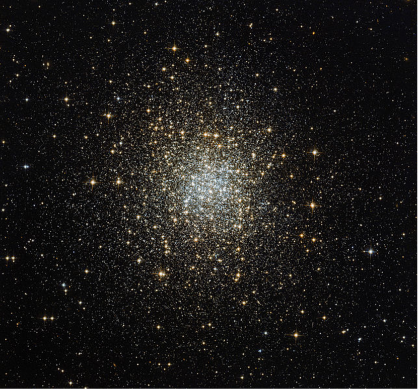
Figure 1: Palomar 2 F606W ($\sim V$) and F814W ($\sim I$) composite image by ESA/Hubble & NASA. North is up and East to the left.

The approach to map - and correct for - the differential reddening basically follows the method described in Bonatto et al. (2013). In summary, in that work the field of view (FoV) of a star cluster was divided in a grid of (fixed-size) cells, from which partial CMDs were extracted and compared with the average CMD (i.e. with all stars in the field). Then it was assumed that morphological differences among the partial CMDs were essentially linear shifts along the reddening vector due to non-uniform dust distribution. In this context, the approach computed the value of $E(B-V)$ that made each partial CMD agree with the average one. Finally, a map was produced for $\delta E(B-V)$, the difference in $E(B-V)$ between each partial CMD and the bluest (that with the least amount of reddening) one.

Although the use of fixed-size cells simplifies the algorithm, in general it leads to oversampling the inner regions, thus lowering the spatial resolution there. Since the stellar surface density of GCs roughly follows a power-law with a core (e.g. King 1962), same-size cells located near the GC center are bound to contain many more stars than those at the outskirts. So, if a minimum number of stars is required to define a CMD, obviously this criterion would be met by a much smaller cell near the center than outwards. Consequently, an improvement to the original approach was introduced so that now variable-size cells are used.

First one sets the minimum number ($N_{min}$) of stars required to roughly define a CMD (this value depends on the quality of the photometry), and the field of view of the GC is divided into 4 quadrants to be individually analysed. Then, if the number of stars in any quadrant is higher than $4\times N_{min}$, a new division by 4 is applied to that quadrant, and so on recursively, until the number of stars in the higher order quadrants gets lower than $4\times N_{min}$. The partial CMDs are then built only for the quadrants having at least $N_{min}$ stars. Figure 2 shows that the number-density of cells basically follows the spatial density of stars across the field of Palomar 2, which increases towards the central parts. Also, the cell dimension decreases towards the central parts because all cells are required to include a minimum number of stars.

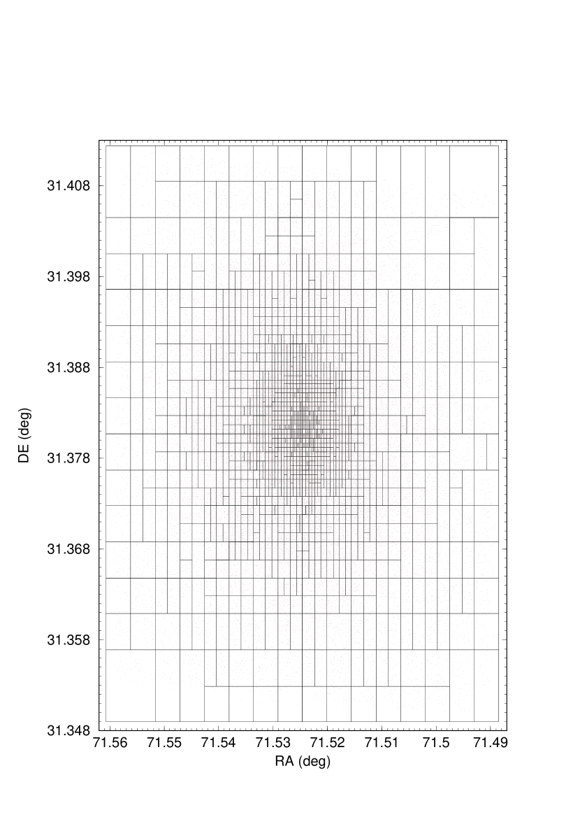
Figure 2: Distribution of the partial CMDs (black polygons) overplotted on the HST WFC/ACS photometry (brown points). The number-density of extracted CMDs increases towards the center following the GC stellar surface density.

Instead of the discrete CMDs, here we use Hess (Hess 1924) diagrams, their continuous analogues that take photometric uncertainties into account. The values of $\delta E(B-V)$ are found by minimizing the residuals of the difference between the average and partial Hess diagrams. Minimization is achieved by means of the global optimisation method Simulated Annealing (SA, Goffe et al. 1994; Bonatto et al. 2012) is used to compute $\delta E(B-V)$.

Once the $\delta E(B-V)$ map has been built, it is straightforward to correct the values of F606W and F814W for each star and produce the differential-reddening corrected CMD (or Hess diagram). This process is illustrated in Fig. 3. Clearly, the relatively heavy differential reddening in Palomar 2 leads to a significant scatter and broadening of the upper main sequence and the evolved sequences - red-giant branch (RGB), horizontal branch (HB) and asymptotic giant branch (AGB) - (Top-right panel). After correction, the scatter gets much reduced and the sequences become better defined (bottom-left). Right panels show the spatial distribution of the density of stars (top), the colour $\mbox{$m_{\rm F606W}$}-\mbox{$m_{\rm F814W}$}$ (middle) and $\delta E(B-V)$ (bottom).

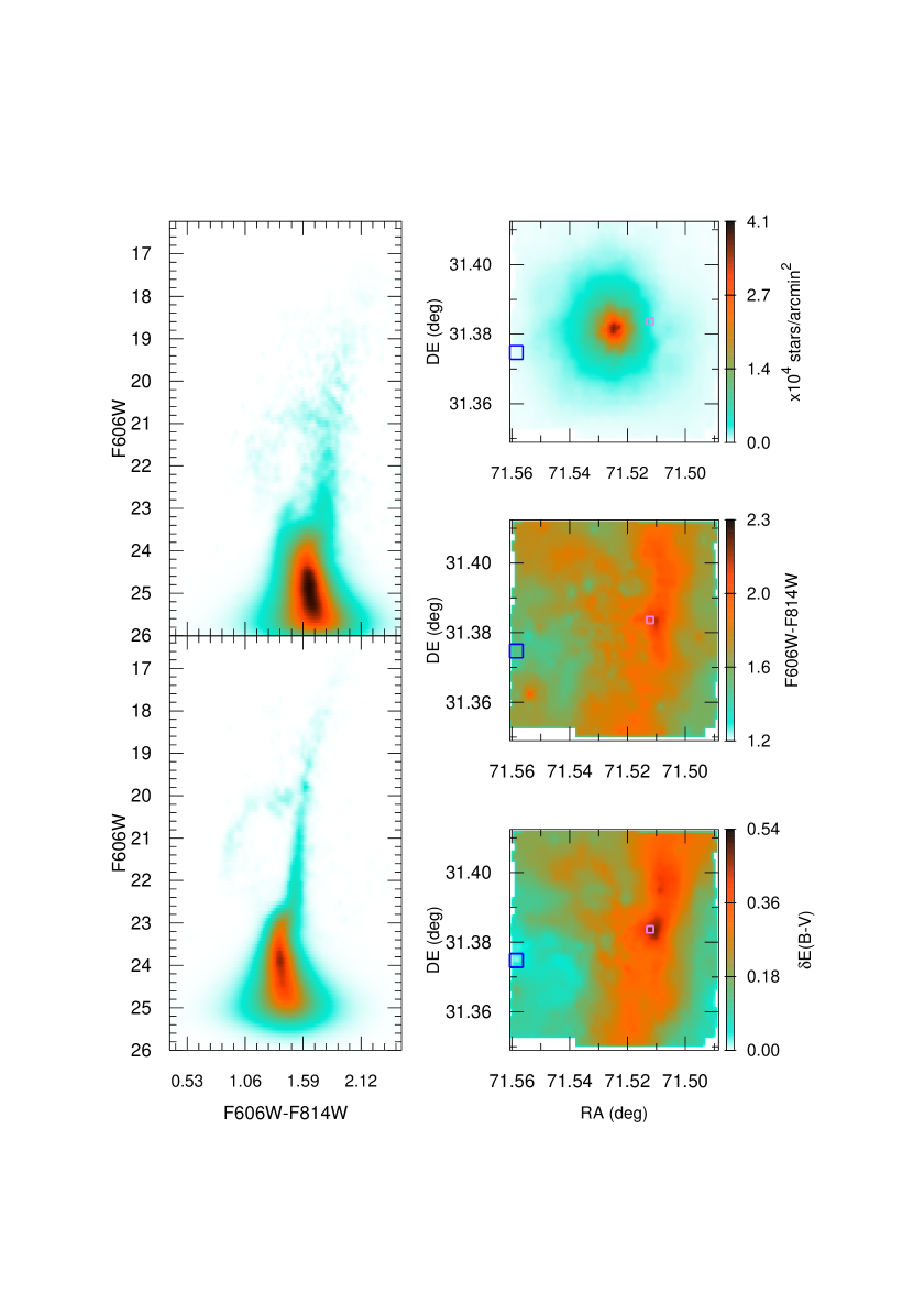
Figure 3: Original (top-left panel) and differentially-reddening corrected photometry (bottom-left) of Palomar 2. Right panels show the stellar surface density (top), colour (middle) and $\delta E(B-V)$ (bottom) spatial distributions. The blue and violet rectangles locate the bluest and reddest cells, respectively.

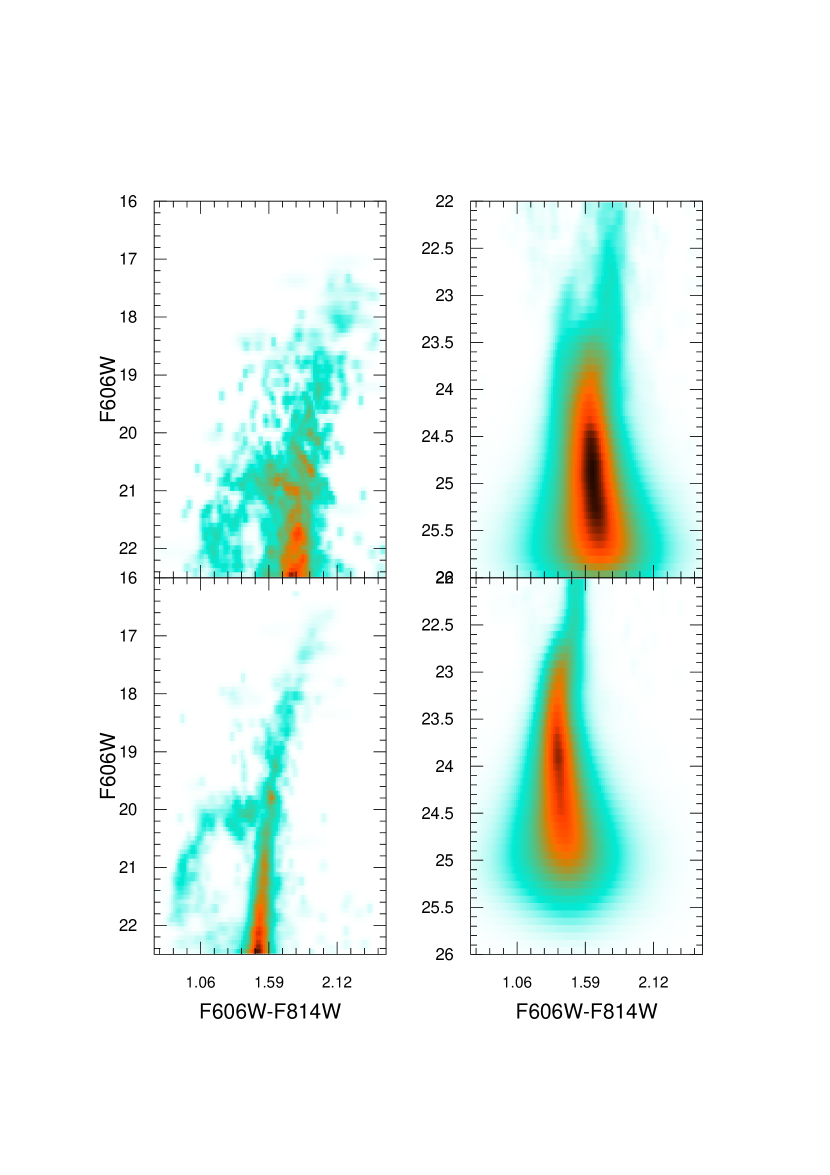
Figure 4: Left panels compare the original (top) and differentially-reddening corrected evolved stellar sequences RGB, HB and AGB (bottom); Right: same for the upper main sequence.

As expected, the spatial distribution of $\delta E(B-V)$ essentially matches that of the colour, especially the nearly South-North dust lane. The location and size of the bluest and reddest CMDs are also shown. The reddest CMD ($\mbox{$\delta E(B-V)$}=0.52$) is located at $RA=71.5122\degr=04^{\rm h}$:$46^{\rm m}$:$2.9^{\rm s}$ and $DE=31.3839\degr=+31\degr$:$23^{\rm m}$:$2^{\rm s}$, while the bluest is at $RA=71.5583\degr=04^{\rm h}$:$46^{\rm m}$:$14^{\rm s}$ and $DE=31.3750\degr=+31\degr$:$22^{\rm m}$:$30^{\rm s}$, near the border of the WFC/ACS field. The average value of the differential reddening across the WFC/ACS field is $\overline{\mbox{$\delta E(B-V)$}}=0.24\pm 0.08$. Such a high value is consistent with the intricate and broad evolutionary sequences seen in the original CMD of Palomar 2 (Fig. 3).

Changes imparted on the stellar sequences by the differential-reddening correction can be better appreciated by zooming in on specific CMD ranges. As shown in Fig. 4, the evolved sequences (left panels) previously barely discernible, now become well defined and tight, displaying beautiful RGB, AGB and a blue-HB, typical of metal-poor GCs. Improvements to the upper main sequence are also quite apparent, especially a better definition of the turn-off (right panels). To better appreciate this improvement, we build the average profiles along the upper main sequence and RGB before and after differential-reddening correction showing the profile amplitude (normalized to the peak value) as a function of the difference in colour ($\delta_{\rm colour}$) with respect to the mean-ridge line at a given magnitude (see Sect. 3 for further details). The average profile width measured across corresponds to 56% of the original profile.

3 Fundamental parameters of Palomar 2

The differential-reddening corrected photometry in the previous Section can now be used to obtain robust fundamental parameters by means of the approach fitCMD, fully described in Bonatto (2019). In summary, the rationale underlying fitCMD is to transpose theoretical initial mass function (IMF) properties - encapsulated by isochrones of given age and metallicity - to their observational counterpart, the CMD. This requires finding values of the total (or cluster) stellar mass, age, global metallicity (Z), foreground reddening, apparent distance modulus, as well as for parameters describing magnitude-dependent photometric completeness. These parameters - including the actual photometric scatter taken from the photometry - are used to build a synthetic CMD that is compared with that of a star cluster. Residual minimization between observed and synthetic CMDs - by means of the global optimization algorithm Simulated Annealing - then leads to the best-fit parameters.

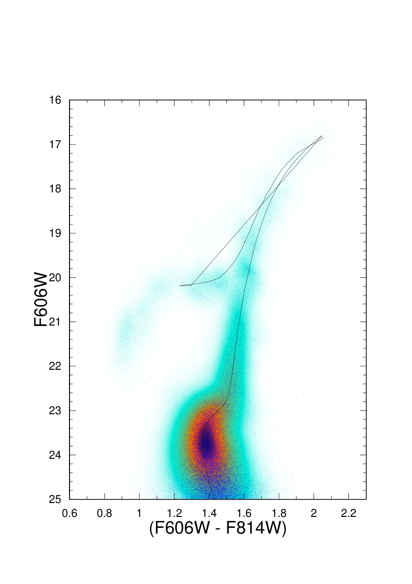
Figure 5: Isochrone fit to the differential-reddening corrected CMD of Palomar 2 according to fitCMD. The best-fit isochrone parameters are: $13.25$ Gyr of age and total metallicity $Z=4\times 10^{-4}$. The actual stars are superimposed on the Hess diagram.

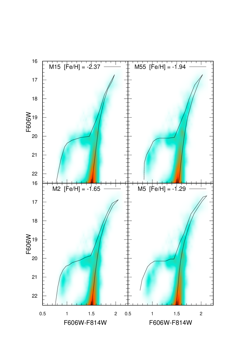
Figure 6: Comparison of the differential-reddening corrected evolved sequences of Palomar 2 with the mean-ridge lines of GCs with different metallicity.

Regarding isochrones, fitCMD employs the latest PARSEC v1.2S$+$COLIBRI PR16 (Bressan et al. 2012; Marigo et al. 2017) models. These isochrones deliver a relatively comprehensive set of fundamental physical parameters for each stellar mass (from the Hydrogen-burning limit to the mass corresponding to stars in highly evolved stages, but still observable in CMDs). Thus, the PARSEC models are quite adequate to build artificial CMDs representative of actual stellar populations.

Since the differential-reddening corrected Hess diagram presents well-defined evolutionary sequences and relatively low photometric scatter, fitCMD readily converged to the best-fit parameters total stellar mass $M=(14\pm 4)\times 10^{4}\,\mbox{$M_{\odot}$}$, the foreground reddening $\mbox{$E(B-V)$}=0.94\pm 0.03$, the intrinsic distance modulus $(m-M)_{0}=17.08\pm 0.13$ (within the uncertainties, both values agree with those given by Sarajedini et al. (2007), the distance to the Sun $\mbox{$d_{\odot}$}=26.1\pm 1.5$ Kpc, and the absolute magnitude $M_{\rm F606W}=-7.8$ (which essentially corresponds to $M_{V}$). Within the uncertainties, the value of $d_{\odot}$ agrees with the $27.2$ distance found by Harris (2010); the same applies to $M_{V}$. The global metallicity is $Z=(4\pm 1)\times 10^{-4}$, which corresponds to $\mbox{$Z/Z_{\odot}$}\approx 0.03$. Since the specific value of $[\alpha/Fe]$ is not known for Palomar 2, we consider the range $0.0\leq[\alpha/Fe]\leq+0.4$ which is typical for outer halo GCs (e.g. Dotter et al. 2011). Thus, the metallicity of Palomar 2 should be in the range $-1.91\leq\mbox{$[Fe/H]$}\leq-1.58$ (with an uncertainty of $\pm 0.08$. This value is considerably more metal poor than previously quoted by Harris (2010), but fully consistent with the values found for other outer halo GCs (Dotter et al. 2011). The best-fit age is $13.25\pm 0.12$ Gyr, again consistent with other outer halo GCs.

The best-fit isochrone (13.25 Gyr of age and $Z=4\times 10^{-4}$) set with the apparent distance modulus $(m-M)_{\rm F606W}=19.73$ and the foreground reddening $E(\rm F606W-F814W)=0.93$ is shown in Fig. 5, superimposed both on the Hess diagram and CMD of Palomar 2. Although PARSEC isochrones lack the blue-HB extension, they still provide an adequate fit to the upper main sequence, RGB and AGB.

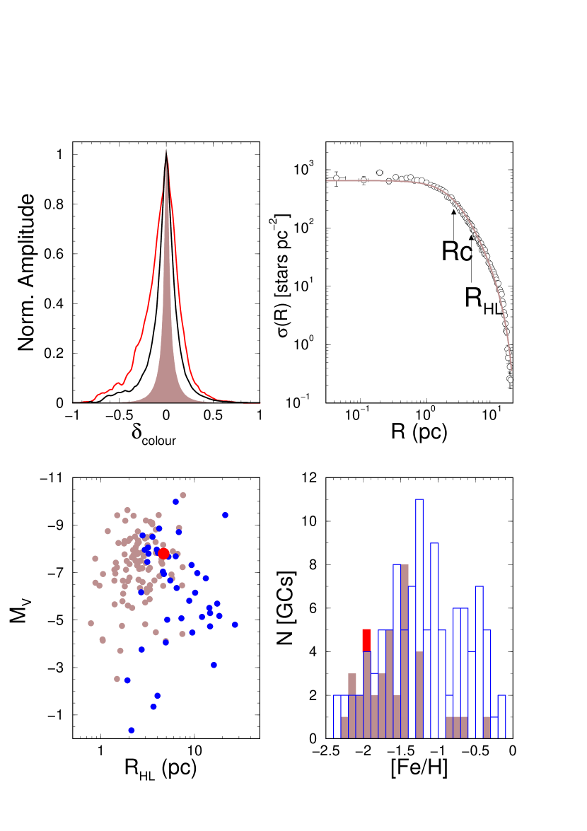
Figure 7: Top-left: average profile along the upper-main sequence and RGB before (red line) and after (black) differential-reddening correction; the profile corresponding to the photometric scattering is shown in brown. Left: radial density profile of Palomar 2 built with the ACS photometry fitted with the 3-parameter King profile (solid line); core and half-light radii are indicated. Bottom-left: $M_{V}\times R_{HL}$ for the outer-halo GCs (blue symbols), the remaining GCs (brown), and Palomar 2 (red). Right: metallicity of Palomar 2 (red) compared to the Milky Way GCs in the outer halo (blue) and the remaining GCs (brown). Since the actual value of $[\alpha/Fe]$ is not known for Palomar 2, we show the range of possible $[Fe/H]$ values corresponding to $0.0\leq[\alpha/Fe]\leq+0.4$.

An alternative way to assess the metallicity of Palomar 2 is by comparing its differential-reddening corrected CMD with those of GCs covering a range in $[Fe/H]$. As quality criteria, the comparison GCs are taken from the same photometric sample as Palomar 2, and their CMDs should have a relatively large number of stars and low reddening (to better define the stellar sequences). Objects satisfying these criteria are M 15 (NGC 7078), $\mbox{$[Fe/H]$}=-2.37$, $\mbox{$E(B-V)$}=0.1$; M 55 (NGC 6809), $\mbox{$[Fe/H]$}=-1.94$, $\mbox{$E(B-V)$}=0.08$; M 2 (NGC 7089), $\mbox{$[Fe/H]$}=-1.65$, $\mbox{$E(B-V)$}=0.06$; and M 5 (NGC 5904), $\mbox{$[Fe/H]$}=-1.29$, $\mbox{$E(B-V)$}=0.03$. In addition, to minimize clutter, the analysis is carried out with the mean-ridge lines of the evolved stellar sequences of the comparison GCs fitted to Palomar 2.

The result is shown in Fig. 6, where the metal-poor nature of Palomar 2 is reinforced. Indeed, the mean-ridge lines of both M 15 and especially M 55 provide an excellent description of the evolved sequences of Palomar 2, thus setting its metallicity to a value closer to $\mbox{$[Fe/H]$}=-1.9$ than $\mbox{$[Fe/H]$}=-1.6$.

Incidentally, Fig. 7 (top-left panel) shows that the differential-reddening corrected profile, although significantly narrower ($\approx 56\%$) than the observed one, is broader than that corresponding to the photometric uncertainties alone. Such excess width might suggest the presence of multiple stellar populations in Palomar 2 (for recent reviews on multiple stellar populations, see Gratton et al. 2012 and Bastian & Lardo 2017). However, it should be noted that the photometric catalogs of Anderson et al. (2008) are affected by unaccounted-for telescope breathing effects, i.e. the change of the PSF shape from one exposure to the next, even within the same HST orbit. This change in the PSF shape can be as large as a few percent, thus introducing systematic photometric errors of about the same amount. In this context, further speculation on the origin of the differential-reddening corrected profile width would require a technically challenging data reduction to include the HST breathing effects, which is beyond the scope of the present paper.

The relatively deep ACS photometry of Palomar 2 was used to build its radial density profile (RDP) (Fig. 7), defined as $\sigma(R)=\frac{dN}{2\pi\,RdR}$. Besides the usual power-law component (in this case for $R\geq 1$ pc), the RDP is quite smooth and presents a relatively flat central region, probably associated with some crowdedness there (see, e.g. Bonatto et al. 2019). To determine structural parameters, the RDP was fitted with the classical three-parameter King (1962) profile, defined as $\sigma(R)=\sigma_{0}\left[\frac{1}{\sqrt{1+(R/\mbox{r${}_{C}$})^{2}}}-\frac{1}{\sqrt{1+(\mbox{r${}_{T}$}/\mbox{r${}_{C}$})^{2})}}\right]^{2}$, where $\sigma_{0}$ is the stellar-density at the center, r_C and r_T are the core and tidal radii, respectively. Parameters derived are $\sigma_{0}=832\pm 25$ stars pc^-2, $\mbox{r${}_{C}$}=0.34\pm 0.01\arcmin=2.6\pm 0.1$ pc, and $\mbox{r${}_{T}$}=2.96\pm 0.05\arcmin=22.5\pm 0.4$ pc. Our value of r_C is about twice that given by Harris (2010), while only about half for r_T  probably because the relatively limited radial range of the ACS photometry.

We also computed its half-light radius as $R_{HL}=0.62\pm 0.02\arcmin$ (somewhat larger than the 0.5′given by Harris 2010), thus implying a physical value of $R_{HL}\approx 4.7$ pc. Incidentally, this value, together with $M_{V}\approx-7.8$, put Palomar 2 right in the middle of the corresponding values spanned by the Milky Way GCs (see, e.g. Fig. 6 in Belokurov et al. 2014). To put these values in context, we compare in Fig. 7 (bottom-left panel) Palomar 2 with the corresponding Milky Way GCs (values taken from Harris 2010) assumed to be in the outer halo (those with Galactocentric distance $R_{GC}>15$ Kpc, e.g. Bica et al. 2006) and the remaining ones. Finally, the range of probable $[Fe/H]$ of Palomar 2 is compared to the corresponding distribution measured in Milky Way GCs (outer-halo and remaining GCs) in the bottom-right panel of Fig. 7. Both comparisons confirm that Palomar 2 is a typical outer-halo GC.

4 Concluding remarks

Because of the deleterious effects associated with differential reddening, CMDs of the scarcely studied globular cluster Palomar 2 have been essentially useless for a more in-depth analysis since its discovery in the 1950s. In this work, Hubble Space Telescope Advanced Camera for Surveys data are used to correct the photometry in F606W and F814W of each star in the field of view of Palomar 2 for differential reddening with a relatively high spatial resolution. CMDs are extracted in different regions across the FoV of Palomar 2, and the differences in $E(B-V)$ among them are used to build a differential reddening map. Finally, correcting the observed values of F606W and F814W for differential reddening of each star leads to a CMD with significantly less photometric scatter and, consequently, well-defined stellar sequences, especially the RGB, HB and AGB.

Parameters derived from the corrected CMD show that Palomar 2 contains a total stellar mass of $M=1.4\times 10^{5}\,\mbox{$M_{\odot}$}$, is affected by the foreground reddening $\mbox{$E(B-V)$}=0.93$, and is located at $\mbox{$d_{\odot}$}=26.1\pm 1.5$ Kpc from the Sun; its absolute magnitude is $M_{V}\approx-7.8$, and its age is $13.25\pm 0.12$ Gyr. The global metallicity is $\mbox{$Z/Z_{\odot}$}\approx 0.03$, which corresponds to $-1.91\leq\mbox{$[Fe/H]$}\leq-1.58$ (for $0.0\leq[\alpha/Fe]\leq+0.4$). Structural parameters are the core and half-light radii $\mbox{r${}_{C}$}\approx 2.6$ pc and $R_{HL}\approx 4.7$ pc, respectively. These values are consistent with other outer halo GCs.

References

- Anderson et al. (2008) Anderson J., et al., 2008, AJ, 135, 2055
- Bastian & Lardo (2017) Bastian N., Lardo C., 2017, preprint, (arXiv:1712.01286)
- Bechtol et al. (2015) Bechtol K., et al., 2015, ApJ, 807, 50
- Belokurov et al. (2014) Belokurov V., Irwin M. J., Koposov S. E., Evans N. W., Gonzalez-Solares E., Metcalfe N., Shanks T., 2014, MNRAS, 441, 2124
- Belokurov et al. (2018) Belokurov V., Erkal D., Evans N. W., Koposov S. E., Deason A. J., 2018, MNRAS, 478, 611
- Bica et al. (2006) Bica E., Bonatto C., Barbuy B., Ortolani S., 2006, A&A, 450, 105
- Bonatto (2019) Bonatto C., 2019, MNRAS, 483, 2758
- Bonatto et al. (2012) Bonatto C., Lima E. F., Bica E., 2012, A&A, 540, A137
- Bonatto et al. (2013) Bonatto C., Campos F., Kepler S. O., 2013, MNRAS, 435, 263
- Bonatto et al. (2019) Bonatto C., et al., 2019, A&A, 622, A179
- Bressan et al. (2012) Bressan A., Marigo P., Girardi L., Salasnich B., Dal Cero C., Rubele S., Nanni A., 2012, MNRAS, 427, 127
- Chatterjee et al. (2013) Chatterjee S., Umbreit S., Fregeau J. M., Rasio F. A., 2013, MNRAS, 429, 2881
- Dotter et al. (2011) Dotter A., Sarajedini A., Anderson J., 2011, ApJ, 738, 74
- Emerson & Sutherland (2010) Emerson J., Sutherland W., 2010, The Messenger, 139, 2
- Forbes & Bridges (2010) Forbes D. A., Bridges T., 2010, MNRAS, 404, 1203
- Gaia Collaboration et al. (2018a) Gaia Collaboration et al., 2018a, A&A, 616, A1
- Gaia Collaboration et al. (2018b) Gaia Collaboration et al., 2018b, A&A, 616, A12
- Goffe et al. (1994) Goffe W. L., Ferrier G. D., Rogers J., 1994, Journal of Econometrics, 60, 65
- Gratton et al. (2012) Gratton R. G., Carretta E., Bragaglia A., 2012, A&ARv, 20, 50
- Harris (2010) Harris W. E., 2010, preprint, (arXiv:1012.3224)
- Harris et al. (1997) Harris W. E., Durrell P. R., Petitpas G. R., Webb T. M., Woodworth S. C., 1997, AJ, 114, 1043
- Helmi et al. (1999) Helmi A., White S. D. M., de Zeeuw P. T., Zhao H., 1999, Nature, 402, 53
- Hess (1924) Hess R., 1924, Probleme der Astronomie. Festschrift fur Hugo v. Seeliger. (Berlin:Springer), p. 265
- Ibata et al. (1994) Ibata R. A., Gilmore G., Irwin M. J., 1994, Nature, 370, 194
- Kalirai & Richer (2010) Kalirai J. S., Richer H. B., 2010, Philosophical Transactions of the Royal Society of London Series A, 368, 755
- King (1962) King I., 1962, AJ, 67, 471
- Leaman et al. (2013) Leaman R., VandenBerg D. A., Mendel J. T., 2013, MNRAS, 436, 122
- Li et al. (2016) Li C.-Y., de Grijs R., Deng L.-C., 2016, Research in Astronomy and Astrophysics, 16, 179
- Li et al. (2019) Li T. S., et al., 2019, MNRAS, 490, 3508
- Marigo et al. (2017) Marigo P., et al., 2017, ApJ, 835, 77
- Massari et al. (2019) Massari D., Koppelman H. H., Helmi A., 2019, A&A, 630, L4
- Mateu et al. (2018) Mateu C., Read J. I., Kawata D., 2018, MNRAS, 474, 4112
- Palma et al. (2019) Palma T., et al., 2019, MNRAS, 487, 3140
- Peñarrubia et al. (2009) Peñarrubia J., Walker M. G., Gilmore G., 2009, MNRAS, 399, 1275
- Sarajedini et al. (2007) Sarajedini A., et al., 2007, AJ, 133, 1658
- Shipp et al. (2018) Shipp N., et al., 2018, ApJ, 862, 114