Do We Need Zero Training Loss After Achieving Zero Training Error?

Abstract

Overparameterized deep networks have the capacity to memorize training data with zero training error. Even after memorization, the training loss continues to approach zero, making the model overconfident and the test performance degraded. Since existing regularizers do not directly aim to avoid zero training loss, it is hard to tune their hyperparameters in order to maintain a fixed/preset level of training loss. We propose a direct solution called flooding that intentionally prevents further reduction of the training loss when it reaches a reasonably small value, which we call the flood level. Our approach makes the loss float around the flood level by doing mini-batched gradient descent as usual but gradient ascent if the training loss is below the flood level. This can be implemented with one line of code and is compatible with any stochastic optimizer and other regularizers. With flooding, the model will continue to “random walk” with the same non-zero training loss, and we expect it to drift into an area with a flat loss landscape that leads to better generalization. We experimentally show that flooding improves performance and, as a byproduct, induces a double descent curve of the test loss.

1 Introduction

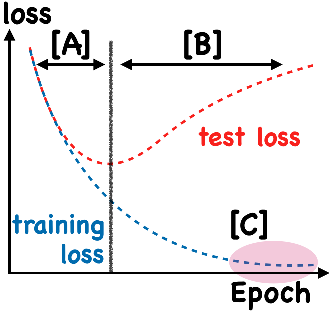
(a) w/o Flooding

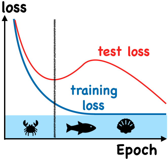
(b) w/ Flooding

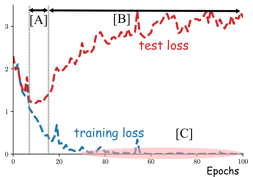
(c) C10 w/o Flooding

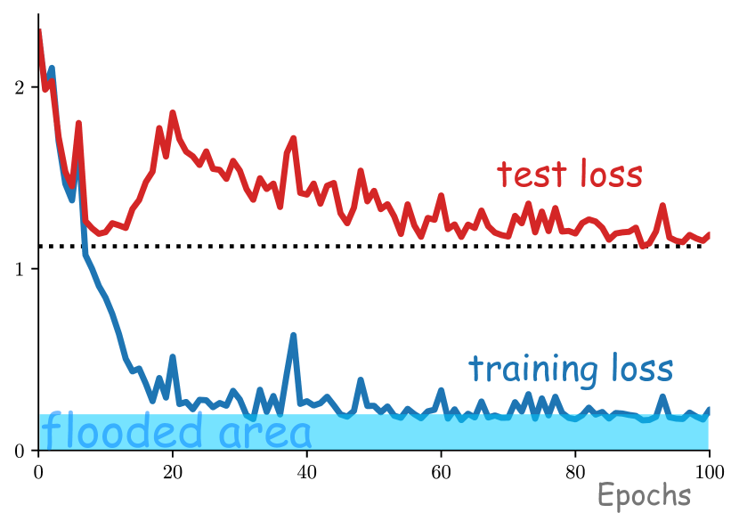
(d) C10 w/ Flooding

Figure 1: (a) shows 3 different concepts related to overfitting. [A] shows the generalization gap increases, while the training and test losses decrease. [B] also shows the increasing gap, but the test loss starts to rise. [C] shows the training loss becoming (near-)zero. We avoid [C] by flooding the bottom area, visualized in (b), which forces the training loss to stay around a constant. This leads to a decreasing test loss once again. We confirm these claims in experiments with CIFAR-10 shown in (c)–(d).

“Overfitting” is one of the biggest interests and concerns in the machine learning community (Ng, 1997; Caruana et al., 2000; Belkin et al., 2018; Roelofs et al., 2019; Werpachowski et al., 2019). One way of identifying overfitting is to see whether the generalization gap, the test minus the training loss, is increasing or not (Goodfellow et al., 2016). We can further decompose the situation of the generalization gap increasing into two stages: The first stage is when both the training and test losses are decreasing, but the training loss is decreasing faster than the test loss ([A] in Fig. 1(a).) The next stage is when the training loss is decreasing, but the test loss is increasing.

Within stage [B], after learning for even more epochs, the training loss will continue to decrease and may become (near-)zero. This is shown as [C] in Fig. 1(a). If we continue training even after the model has memorized (Zhang et al., 2017; Arpit et al., 2017; Belkin et al., 2018) the training data completely with zero error, the training loss can easily become (near-)zero especially with overparametrized models. Recent works on overparametrization and double descent curves (Belkin et al., 2019; Nakkiran et al., 2020) have shown that learning until zero training error is meaningful to achieve a lower generalization error. However, whether zero training loss is necessary after achieving zero training error remains an open issue.

In this paper, we propose a method to make the training loss float around a small constant value, in order to prevent the training loss from approaching zero. This is analogous to flooding the bottom area with water, and we refer to the constant value as the flood level. Note that even if we add flooding, we can still memorize the training data. Our proposal only forces the training loss to become positive, which does not necessarily mean the training error will become positive, as long as the flood level is not too large. The idea of flooding is shown in Fig. 1(b), and we show learning curves before and after flooding with a benchmark dataset in Fig. 1(c) and Fig. 1(d).

Algorithm and implementation

Our algorithm of flooding is surprisingly simple. If the original learning objective is $J$, the proposed modified learning objective $\widetilde{J}$ with flooding is

$$\widetilde{J}(\bm{\theta})=|J(\bm{\theta})-b|+b,$$ (1)

where $b>0$ is the flood level specified by the user, and $\bm{\theta}$ is the model parameter.

The gradient of $\tilde{J}$ w.r.t. $\bm{\theta}$ will point in the same direction as that of $J(\bm{\theta})$ when $J(\bm{\theta})>b$ but in the opposite direction when $J(\bm{\theta})<b$. This means that when the learning objective is above the flood level, there is a “gravity” effect with gradient descent, but when the learning objective is below the flood level, there is a “buoyancy” effect with gradient ascent. In practice, this will be performed with a mini-batch and will be compatible with any stochastic optimizers. It can also be used along with other regularization methods.

During flooding, the training loss will repeat going below and above the flood level. The model will continue to “random walk” with the same non-zero training loss, and we expect it to drift into an area with a flat loss landscape that leads to better generalization (Hochreiter & Schmidhuber, 1997; Chaudhari et al., 2017; Keskar et al., 2017; Li et al., 2018). In experiments, we show that during this period of random walk, there is an increase in flatness of the loss function (See Section 5.3).

This modification can be incorporated into existing machine learning code easily: Add one line of code for Eq. (1) after evaluating the original objective function $J(\bm{\theta})$. A minimal working example with a mini-batch in PyTorch (Paszke et al., 2019) is demonstrated below to show the additional one line of code:

⬇

1outputs = model(inputs)

2loss = criterion(outputs, labels)

3flood = (loss-b).abs()+b # This is it!

4optimizer.zero_grad()

5flood.backward()

6optimizer.step()

It may be hard to set the flood level without expert knowledge on the domain or task. We can circumvent this situation easily by treating the flood level as a hyper-parameter. We may exhaustively evaluate the accuracy for the predefined hyper-parameter candidates with a validation dataset, which can be performed in parallel.

Previous regularization methods

Many previous regularization methods also aim at avoiding training too much in various ways including restricting the parameter norm to become small by decaying the parameter weights (Hanson & Pratt, 1988), raising the difficulty of training by dropping activations of neural networks (Srivastava et al., 2014), avoiding the model to output a hard label by smoothing the training labels (Szegedy et al., 2016), and simply stopping training at an earlier phase (Morgan & Bourlard, 1990). These methods can be considered as indirect ways to control the training loss, by also introducing additional assumptions such as the optimal model parameters are close to zero. Although making the regularization effect stronger would make it harder for the training loss to approach zero, it is still hard to maintain the right level of training loss till the end of training. In fact, for overparametrized deep networks, applying small regularization would not stop the training loss becoming (near-)zero, making it even harder to choose a hyper-parameter that corresponds to a specific level of loss.

Flooding, on the other hand, is a direct solution to the issue that the training loss becomes (near-)zero. Flooding intentionally prevents further reduction of the training loss when it reaches a reasonably small value, and the flood level corresponds to the level of training loss that the user wants to keep.

Table 1: Conceptual comparisons of various regularizers. “Indep.”/“tr.” stands for “independent”/“training” and $\checkmark$/$\times$ stands for yes/no.

Regularization and other methods	Target tr. loss	Domain indep.	Task indep.	Model indep.	Main assumption
$\ell_{2}$ regularization (Tikhonov, 1943)	$\times$	$\checkmark$	$\checkmark$	$\checkmark$	Optimal model params are close to 0
Weight decay (Hanson & Pratt, 1988)	$\times$	$\checkmark$	$\checkmark$	$\checkmark$	Optimal model params are close to 0
Early stopping (Morgan & Bourlard, 1990)	$\times$	$\checkmark$	$\checkmark$	$\checkmark$	Overfitting occurs in later epochs
$\ell_{1}$ regularization (Tibshirani, 1996)	$\times$	$\checkmark$	$\checkmark$	$\checkmark$	Optimal model has to be sparse
Dropout (Srivastava et al., 2014)	$\times$	$\checkmark$	$\checkmark$	$\times$	Existence of complex co-adaptations
Batch normalization (Ioffe & Szegedy, 2015)	$\times$	$\checkmark$	$\checkmark$	$\times$	Existence of internal covariate shift
Label smoothing (Szegedy et al., 2016)	$\times$	$\checkmark$	$\times$	$\checkmark$	True posterior is not a one-hot vector
Mixup (Zhang et al., 2018)	$\times$	$\times$	$\times$	$\checkmark$	Linear relationship between $\bm{x}$ and $y$
Image augment. (Shorten & Khoshgoftaar, 2019)	$\times$	$\times$	$\checkmark$	$\checkmark$	Input is invariant to the translations
Flooding (proposed method)	$\checkmark$	$\checkmark$	$\checkmark$	$\checkmark$	Learning until zero loss is harmful

2 Backgrounds

In this section, we review regularization methods (summarized in Table 1), recent works on overparametrization and double descent curves, and the area of weakly supervised learning where similar techniques to flooding have been explored.

2.1 Regularization Methods

The name “regularization” dates back to at least Tikhonov regularization for the ill-posed linear least-squares problem (Tikhonov, 1943; Tikhonov & Arsenin, 1977). One example is to modify $\bm{X}^{\top}\bm{X}$ (where $\bm{X}$ is the design matrix) to become “regular” by adding a term to the objective function. $\ell_{2}$ regularization is a generalization of the above example and can be applied to non-linear models. These methods implicitly assume that the optimal model parameters are close to zero.

It is known that weight decay (Hanson & Pratt, 1988), dropout (Srivastava et al., 2014), and early stopping (Morgan & Bourlard, 1990) are equivalent to $\ell_{2}$ regularization under certain conditions (Loshchilov & Hutter, 2019; Bishop, 1995; Goodfellow et al., 2016; Wager et al., 2013), implying that they have similar assumptions on the optimal model parameters. There are other penalties based on different assumptions such as the $\ell_{1}$ regularization (Tibshirani, 1996) based on the sparsity assumption that the optimal model has only a few non-zero parameters.

Modern machine learning tasks are applied to complex problems where the optimal model parameters are not necessarily close to zero or are not sparse, and it would be ideal if we can properly add regularization effects to the optimization stage without such assumptions. Our proposed method does not have assumptions on the optimal model parameters and can be useful for more complex problems.

More recently, “regularization” has further evolved to a more general meaning including various methods that alleviate overfitting but do not necessarily have a step to regularize a singular matrix or add a regularization term to the objective function. For example, Goodfellow et al. (2016) defines regularization as “any modification we make to a learning algorithm that is intended to reduce its generalization error but not its training error.” In this paper, we adopt this broader meaning of “regularization.”

Examples of the more general regularization category include mixup (Zhang et al., 2018) and data augmentation methods like cropping, flipping, and adjusting brightness or sharpness (Shorten & Khoshgoftaar, 2019). These methods have been adopted in many state-of-the-art methods (Verma et al., 2019; Berthelot et al., 2019; Kolesnikov et al., 2020) and are becoming essential regularization tools for developing new systems. However, these regularization methods have the drawback of being domain-specific: They are designed for the vision domain and require some efforts when applying to other domains (Guo et al., 2019; Thulasidasan et al., 2019). Other regularizers such as label smoothing (Szegedy et al., 2016) is used for problems with class labels and harder to use with regression or ranking, meaning that they are task-specific. Batch normalization (Ioffe & Szegedy, 2015) and dropout (Srivastava et al., 2014) are designed for neural networks and are model-specific.

Although these regularization methods—both the special and general ones—already work well in practice and have become the de facto standard tools (Bishop, 2011; Goodfellow et al., 2016), we provide an alternative which is even more general in the sense that it is domain-, task-, and model-independent.

That being said, we want to emphasize that the most important difference between flooding and other regularization methods is whether it is possible to target a specific level of training loss other than zero. While flooding allows the user to choose the level of training loss directly, it is hard to achieve this with other regularizers.

2.2 Double Descent Curves with Overparametrization

Recently, there has been increasing attention on the phenomenon of “double descent,” named by Belkin et al. (2019), to explain the two regimes of deep learning: The first one (underparametrized regime) occurs where the model complexity is small compared to the number of samples, and the test error as a function of model complexity decreases with low model complexity but starts to increase after the model complexity is large enough. This follows the classical view of machine learning that excessive complexity leads to poor generalization. The second one (overparametrized regime) occurs when an even larger model complexity is considered. Then increasing the complexity only decreases test error, which leads to a double descent shape. The phase of decreasing test error often occurs after the training error becomes zero. This follows the modern view of machine learning that bigger models lead to better generalization.

As far as we know, the discovery of double descent curves dates back to at least Krogh & Hertz (1992), where they theoretically showed the double descent phenomenon under a linear regression setup. Recent works (Belkin et al., 2019; Nakkiran et al., 2020) have shown empirically that a similar phenomenon can be observed with deep learning methods. Nakkiran et al. (2020) observed that the double descent curves for the test error can be shown not only as a function of model complexity, but also as a function of the epoch number.

To the best of our knowledge, the epoch-wise double descent curve was not observed for the test loss before but was observed in our experiments after using flooding with only about 100 epochs. Investigating the connection between epoch-wise double descent curves for the test loss and previous double descent curves (Krogh & Hertz, 1992; Belkin et al., 2019; Nakkiran et al., 2020) is out of the scope of this paper but is an important future direction.

2.3 Avoiding Over-Minimization of the Empirical Risk

It is commonly observed that the empirical risk goes below zero, and it causes overfitting (Kiryo et al., 2017) in weakly supervised learning when an equivalent form of the risk expressed with the given weak supervision is alternatively used (Natarajan et al., 2013; Cid-Sueiro et al., 2014; du Plessis et al., 2014, 2015; Patrini et al., 2017; van Rooyen & Williamson, 2018). Kiryo et al. (2017) proposed a gradient ascent technique to keep the empirical risk non-negative. This idea has been generalized and applied to other weakly supervised settings (Han et al., 2020; Ishida et al., 2019; Lu et al., 2020).

Although we also set a lower bound on the empirical risk, the motivation is different: First, while Kiryo et al. (2017) and others aim to fix the negative empirical risk to become non-negative, our original empirical risk is already non-negative. Instead, we are aiming to sink the original empirical risk by modifying it with a positive lower bound. Second, the problem settings are different. Weakly supervised learning methods require certain loss corrections or sample corrections (Han et al., 2020) before the non-negative correction, but we work on the original empirical risk without any setting-specific modifications.

Early stopping (Morgan & Bourlard, 1990) may be a naive solution to this problem where the empirical risk becomes too small. However, performance of early stopping highly depends on the training dynamics and is sensitive to the randomness in the optimization method and mini-batch sampling. This suggests that early stopping at the optimal epoch in terms of a single training path does not necessarily perform well in another round of training. This makes it difficult to use hyper-parameter selection techniques such as cross-validation that requires re-training a model more than once. In our experiments, we will demonstrate how flooding performs even better than early stopping.

3 Flooding: How to Avoid Zero Training Loss

In this section, we propose our regularization method, flooding. Note that this section and the following sections only consider multi-class classification for simplicity.

3.1 Preliminaries

Consider input variable $\bm{x}\in\mathbb{R}^{d}$ and output variable $y\in[K]:=\{1,\ldots,K\}$, where $K$ is the number of classes. They follow an unknown joint probability distribution with density $p(\bm{x},y)$. We denote the score function by $\bm{g}:\mathbb{R}^{d}\rightarrow\mathbb{R}^{K}$. For any test data point $\bm{x}_{0}$, our prediction of the output label will be given by $\widehat{y}_{0}:=\operatorname*{\mathrm{arg\,max}}_{z\in[K]}g_{z}(\bm{x}_{0})$, where $g_{z}(\cdot)$ is the $z$-th element of $\bm{g}(\cdot)$, and in case of a tie, $\operatorname*{\mathrm{arg\,max}}$ returns the largest argument. Let $\ell:\mathbb{R}^{K}\times[K]\rightarrow\mathbb{R}$ denote a loss function. $\ell$ can be the zero-one loss,

$$\ell_{01}(\bm{v},z^{\prime}):=\begin{cases}0&\text{if}\quad\operatorname*{\mathrm{arg\,max}}_{z\in\{1,\dots,K\}}v_{z}=z^{\prime},\\ 1&\text{otherwise},\end{cases}$$ (2)

where $\bm{v}:=(v_{1},\dots,v_{K})^{\top}\in\mathbb{R}^{K}$, or a surrogate loss such as the softmax cross-entropy loss,

$$\ell_{\text{CE}}(\bm{v},z^{\prime}):=-\log\frac{\exp(v_{z^{\prime}})}{\sum_{z\in[K]}\exp(v_{z})}.$$ (3)

For a surrogate loss $\ell$, we denote the classification risk by

$$R(\bm{g}):=\mathbb{E}_{p(\bm{x},y)}[\ell(\bm{g}(\bm{x}),y)]$$ (4)

where $\mathbb{E}_{p(\bm{x},y)}[\cdot]$ is the expectation over $(\bm{x},y)\sim p(\bm{x},y)$. We use $R_{01}(\bm{g})$ to denote Eq. (4) when $\ell=\ell_{01}$ and call it the classification error.

The goal of multi-class classification is to learn $\bm{g}$ that minimizes the classification error $R_{01}(\bm{g})$. In optimization, we consider the minimization of the risk with a almost surely differentiable surrogate loss $R(\bm{g})$ instead to make the problem more tractable. Furthermore, since $p(\bm{x},y)$ is usually unknown and there is no way to exactly evaluate $R(\bm{g})$, we minimize its empirical version calculated from the training data instead:

$$\widehat{R}(\bm{g}):=\frac{1}{n}\sum^{n}_{i=1}\ell(\bm{g}(\bm{x}_{i}),y_{i}),$$ (5)

where $\{(\bm{x}_{i},y_{i})\}_{i=1}^{n}$ are i.i.d. sampled from $p(\bm{x},y)$. We call $\widehat{R}$ the empirical risk.

We would like to clarify some of the undefined terms used in the title and the introduction. The “train/test loss” is the empirical risk with respect to the surrogate loss function $\ell$ over the training/test data, respectively. We refer to the “training/test error” as the empirical risk with respect to $\ell_{01}$ over the training/test data, respectively (which is equal to one minus accuracy) (Zhang, 2004).

Finally, we formally define the Bayes risk as

$$R^{*}:=\inf_{\bm{h}}R(\bm{h}),$$

where the infimum is taken over all measurable, vector-valued functions $\bm{h}\colon\mathbb{R}^{d}\to\mathbb{R}^{K}$. The Bayes risk is often referred to as the Bayes error if the zero-one loss is used:

$$\inf_{\bm{h}}R_{01}(\bm{h}).$$

3.2 Algorithm

With flexible models, $\widehat{R}(\bm{g})$ w.r.t. a surrogate loss can easily become small if not zero, as we mentioned in Section 1; see [C] in Fig. 1(a). We propose a method that “floods the bottom area and sinks the original empirical risk” as in Fig. 1(b) so that the empirical risk cannot go below the flood level. More technically, if we denote the flood level as $b$, our proposed training objective with flooding is a simple fix.

Definition 1.

The flooded empirical risk is defined as

$$\widetilde{R}(\bm{g})=|\widehat{R}(\bm{g})-b|+b.$$ (6)

Note that when $b=0$, then $\widetilde{R}(\bm{g})=\widehat{R}(\bm{g})$. The gradient of $\widetilde{R}(\bm{g})$ w.r.t. model parameters will point to the same direction as that of $\widehat{R}(\bm{g})$ when $\widehat{R}(\bm{g})>b$ but in the opposite direction when $\widehat{R}(\bm{g})<b$. This means that when the learning objective is above the flood level, we perform gradient descent as usual (gravity zone), but when the learning objective is below the flood level, we perform gradient ascent instead (buoyancy zone).

The issue is that in general, we seldom know the optimal flood level in advance. This issue can be mitigated by searching for the optimal flood level $b^{*}$ with a hyper-parameter optimization technique. In practice, we can search for the optimal flood level by performing the exhaustive search in parallel.

3.3 Implementation

For large scale problems, we can employ mini-batched stochastic optimization for efficient computation. Suppose that we have $M$ disjoint mini-batch splits. We denote the empirical risk (5) with respect to the $m$-th mini-batch by $\widehat{R}_{m}(\bm{g})$ for $m\in\{1,\ldots,M\}$. Our mini-batched optimization performs gradient descent updates in the direction of the gradient of $\lvert\widehat{R}_{\mathrm{m}}(\bm{g})-b\rvert+b$. By the convexity of the absolute value function and Jensen’s inequality, we have

$$\widetilde{R}(\bm{g})\leq\frac{1}{M}\sum_{m=1}^{M}\left(\lvert\widehat{R}_{\mathrm{m}}(\bm{g})-b\rvert+b\right).$$ (7)

This indicates that mini-batched optimization will simply minimize an upper bound of the full-batch case with $\widetilde{R}(\bm{g})$.

Table 2: Experimental results for the synthetic data. The average and standard deviation of the accuracy of each method over $10$ trials. Sub-table (A) shows the results without early stopping. Sub-table (B) shows the results with early stopping. The boldface denotes the best and comparable method in terms of the average accuracy according to the t-test at the significance level $1\%$. The average and standard deviation of the chosen flood level is also shown.

		(A) Without Early Stopping			(B) With Early Stopping
Data	Label Noise	Without Flooding	With Flooding	Chosen $b$	Without Flooding	With Flooding	Chosen $b$
Two Gaussians	Low	90.52% (0.71)	92.13% (0.48)	0.17 (0.10)	90.41% (0.98)	92.13% (0.52)	0.16 (0.12)
	Middle	84.79% (1.23)	88.03% (1.00)	0.22 (0.09)	85.85% (2.07)	88.15% (0.72)	0.23 (0.08)
	High	78.44% (0.92)	83.59% (0.92)	0.32 (0.08)	81.09% (2.23)	83.87% (0.65)	0.32 (0.11)
Spiral	Low	97.72% (0.26)	98.72% (0.20)	0.03 (0.01)	97.72% (0.68)	98.26% (0.50)	0.02 (0.01)
	Middle	89.94% (0.59)	93.90% (0.90)	0.12 (0.03)	91.37% (1.43)	93.51% (0.84)	0.10 (0.04)
	High	82.38% (1.80)	87.64% (1.60)	0.24 (0.05)	84.48% (1.52)	88.01% (0.82)	0.22 (0.06)
Sinusoid	Low	94.62% (0.89)	94.66% (1.35)	0.05 (0.04)	94.52% (0.85)	95.42% (1.13)	0.03 (0.03)
	Middle	87.85% (1.02)	90.19% (1.41)	0.11 (0.07)	90.56% (1.46)	91.16% (1.38)	0.13 (0.07)
	High	78.47% (2.39)	85.78% (1.34)	0.25 (0.08)	83.88% (1.49)	85.10% (1.34)	0.22 (0.10)

Table 3: Benchmark datasets. Reporting accuracy for all combinations of early stopping and flooding. We compare “w/o flood” and “w/ flood” and the better one is shown in boldface. The best setup for each dataset is shown with underline. “–” means that flood level of zero was optimal. “LR” stands for learning rate and “aug.” is an abbreviation of augmentation.

		w/o early stopping		w/ early stopping
Dataset	Model & Setup	w/o flood	w/ flood	w/o flood	w/ flood
MNIST	MLP	98.45%	98.76%	98.48%	98.66%
	MLP w/ weight decay	98.53%	98.58%	98.51%	98.64%
	MLP w/ batch normalization	98.60%	98.72%	98.66%	98.65%
Kuzushiji	MLP	92.27%	93.15%	92.24%	92.90%
	MLP w/ weight decay	92.21%	92.53%	92.24%	93.15%
	MLP w/ batch normalization	92.98%	93.80%	92.81%	93.74%
SVHN	ResNet18	92.38%	92.78%	92.41%	92.79%
	ResNet18 w/ weight decay	93.20%	–	92.99%	93.42%
CIFAR-10	ResNet44	75.38%	75.31%	74.98%	75.52%
	ResNet44 w/ data aug. & LR decay	88.05%	89.61%	88.06%	89.48%
CIFAR-100	ResNet44	46.00%	45.83%	46.87%	46.73%
	ResNet44 w/ data aug. & LR decay	63.38%	63.70%	63.24%	–

(a) MNIST, MLP

(b) KMNIST, MLP

(c) SVHN, ResNet18

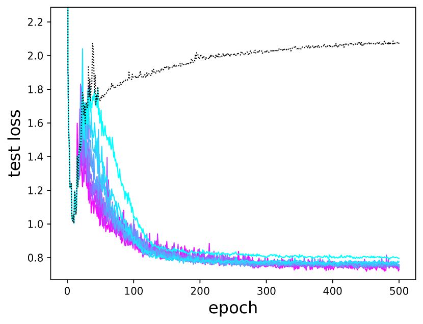
(d) C10, ResNet44

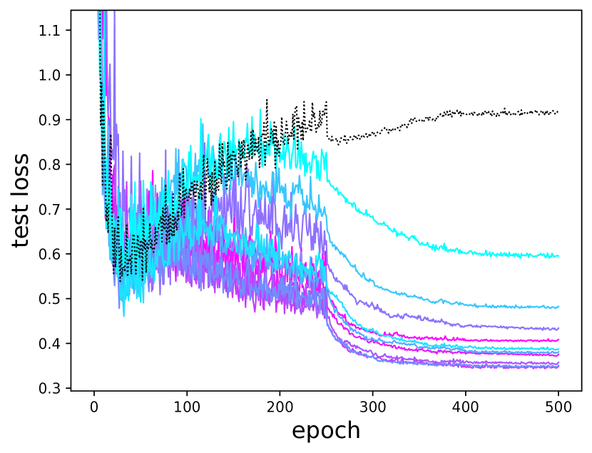
(e) C10, ResNet44, DA & LRD

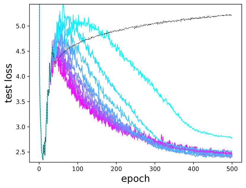
(f) C100, ResNet44

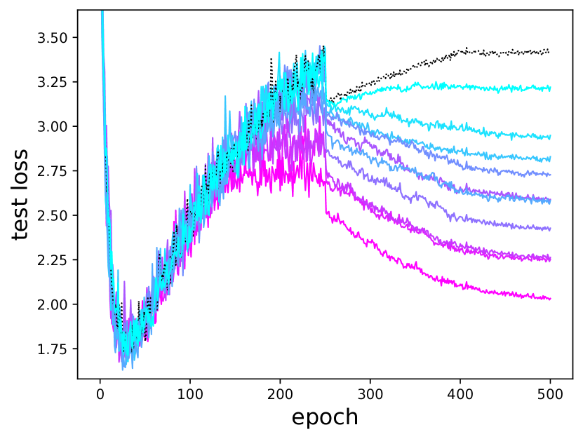
(g) C100, ResNet44, DA & LRD

Figure 2: Learning curves of test loss. The black dotted line shows the baseline without flooding. The colored lines show the results for different flooding levels specified by the color bar. DA and LRD stand for data augmentation and learning rate decay, respectively. We can observe that adding flooding will lead to lower test loss with a double descent curve in most cases. See Fig. 6 in Appendix for other datasets.

4 Does Flooding Generalize Better?

In this section, we show experimental results to demonstrate that adding flooding leads to better generalization. The implementation in this section and the next is based on PyTorch (Paszke et al., 2019) and demo code is available. Experiments were carried out with NVIDIA GeForce GTX 1080 Ti, NVIDIA Quadro RTX 5000 and Intel Xeon Gold 6142.

4.1 Synthetic Datasets

The aim of synthetic experiments is to study the behavior of flooding with a controlled setup.

Data

We use three types of synthetic data: Two Gaussians, Sinusoid (Nakkiran et al., 2019), and Spiral (Sugiyama, 2015). Below we explain how these data were generated.

Two Gaussians Data: We used two $10$-dimensional Gaussian distributions (one for each class) with covariance matrix identity and means $\mu_{\mathrm{P}}=[0,0,\ldots,0]^{\top}$ and $\mu_{\mathrm{N}}=[m,m,\ldots,m]^{\top}$, where $m=1.0$. The training, validation, and test sample sizes are $100$, $100$, and $20000$, respectively.

Sinusoid Data: The sinusoid data (Nakkiran et al., 2019) are generated as follows. We first draw input data points from the $2$-dimensional standard Gaussian distribution, i.e., $\bm{x}\sim N(\bm{0}_{2},\bm{I}_{2})$, where $\bm{0}_{2}$ is the two-dimensional zero vector, and $\bm{I}_{2}$ $2\times 2$ identity matrix. Then put class labels based on

$$y=\mathrm{sign}(\bm{x}^{\top}\bm{w}+\sin(\bm{x}^{\top}\bm{w^{\prime}})),$$

where $\bm{w}$ and $\bm{w^{\prime}}$ are any two $2$-dimesional vectors such that $\bm{w}\perp\bm{w^{\prime}}$. The training, validation, and test sample sizes are $100$, $100$, and $20000$, respectively.

Spiral Data: The spiral data (Sugiyama, 2015) is two-dimensional synthetic data. Let $\theta^{+}_{1}:=0,\theta^{+}_{2},\dots,\theta^{+}_{n^{+}}:=4\pi$ be equally spaced $n^{+}$ points in the interval $[0,4\pi]$, and $\theta^{-}_{1}:=0,\theta^{-}_{2},\dots,\theta^{-}_{n^{-}}:=4\pi$ be equally spaced $n^{-}$ points in the interval $[0,4\pi]$. Let positive and negative input data points be

$$\bm{x}^{+}_{i} :=\theta_{i}[\cos(\theta_{i}),\sin(\theta_{i})]^{\top}+\tau\bm{\nu}^{+}_{i},$$

$$\bm{x}^{-}_{i} :=(\theta+\pi)[\cos(\theta),\sin(\theta)]^{\top}+\tau\bm{\nu}^{-}_{i}$$

for $i=1,\dots,n$, where $\tau$ controls the magnitude of the noise, $\bm{\nu}^{+}_{i}$ and $\bm{\nu}^{-}_{i}$ are i.i.d. distributed according to the two-dimensional standard normal distribution. Then, we make data for classification by $\{(\bm{x}_{i},y_{i})\}_{i=1}^{n}:=\{(\bm{x}^{+}_{i},+1)\}_{i^{+}=1}^{n^{+}}\cup\{(\bm{x}^{-}_{i},-1)\}_{i^{-}=1}^{n^{-}}$, where $n:=n^{+}+n^{-}$. The training, validation, and test sample sizes are $100$, $100$, and $10000$ per class respectively.

Settings

We use a five-hidden-layer feedforward neural network with $500$ units in each hidden layer with the ReLU activation function (Nair & Hinton, 2010). We train the network for $500$ epochs with the logistic loss and the Adam (Kingma & Ba, 2015) optimizer with $100$ mini-batch size and learning rate of $0.001$. The flood level is chosen from $b\in\{0,0.01,0.01,\ldots,0.50\}$. We tried adding label noise to dataset, by flipping $1\%$ (Low), $5\%$ (Middle), or $10\%$ (High) of the labels randomly. This label noise corresponds to varying the Bayes risk, i.e., the difficulty of classification. Note that the training with $b=0$ is identical to the baseline method without flooding. We report the test accuracy of the flood level with the best validation accuracy. We first conduct experiments without early stopping, which means that the last epoch was chosen for all flood levels.

Results

The average and standard deviation of the accuracy of each method over $10$ trials are summarized in Table 2. It is worth noting that the average of the chosen flood level $b$ is larger for the larger label noise because the increase of label noise is expected to increase the Bayes risk. This implies the positive correlation between the optimal flood level and the Bayes risk.

From (A) in Table 2, we can see that the method with flooding often improves test accuracy over the baseline method without flooding. As we mentioned in the introduction, it can be harmful to keep training a model until the end without flooding. However, with flooding, the model at the final epoch has good prediction performance according to the results, which implies that flooding helps the late-stage training improve test accuracy.

We also conducted experiments with early stopping, meaning that we chose the model that recorded the best validation accuracy during training. The results are reported in sub-table (B) of Table 2. Compared with sub-table (A), we see that early stopping improves the baseline method without flooding in many cases. This indicates that training longer without flooding was harmful in our experiments. On the other hand, the accuracy for flooding combined with early stopping is often close to that with early stopping, meaning that training until the end with flooding tends to be already as good as doing so with early stopping. The table shows that flooding often improves or retains the test accuracy of the baseline method without flooding even after deploying early stopping. Flooding does not hurt performance but can be beneficial for methods used with early stopping.

4.2 Benchmark Experiments

We next perform experiments with benchmark datasets. Not only do we compare with the baseline without flooding, we also compare or combine with other general regularization methods, which are early stopping and weight decay.

Settings

We use the following benchmark datasets: MNIST, Kuzushiji-MNIST, SVHN, CIFAR-10, and CIFAR-100. The details of the benchmark datasets can be found in Appendix B. Stochastic gradient descent (Robbins & Monro, 1951) is used with learning rate of 0.1 and momentum of 0.9 for 500 epochs. For MNIST and Kuzushiji-MNIST, we use a two-hidden-layer feedforward neural network with 1000 units and the ReLU activation function (Nair & Hinton, 2010). We also compared adding batch normalization (Ioffe & Szegedy, 2015). For SVHN, we used ResNet-18 from He et al. (2016) with the implementation provided in Paszke et al. (2019). For MNIST, Kuzushiji-MNIST, and SVHN, we compared adding weight decay with rate $1\times 10^{-5}$. For CIFAR-10 and CIFAR-100, we used ResNet-44 from He et al. (2016) with the implementation provided in Idelbayev (2020). For CIFAR-10 and CIFAR-100, we compared adding simple data augmentation (random crop and horizontal flip) and learning rate decay (multiply by 0.1 after 250 and 400 epochs). We split the original training dataset into training and validation data with with a proportion of $80:20$ except for when we used data augmentation, we used $85:15$. We perform the exhaustive hyper-parameter search for the flood level with candidates from $\{0.00,0.01,\ldots,0.10\}$. We used the original labels and did not add label noise. We deployed early stopping in the same way as in Section 4.1.

Results

We show the results in Table 3. For each dataset, the best performing setup and combination of regularizers always use flooding. Combining flooding with early stopping, weight decay, data augmentation, batch normalization, and/or learning rate decay usually has complementary effects. As a byproduct, we were able to produce a double descent curve for the test loss with a relatively few number of epochs, shown in Fig. 2.

5 Why Does Flooding Generalize Better?

In this section, we investigate four key properties of flooding to seek potential reasons for better generalization.

5.1 Memorization

Can we maintain memorization (Zhang et al., 2017; Arpit et al., 2017; Belkin et al., 2018) even after adding flooding? We investigate if the trained model has zero training error (100% accuracy) for the flood level that was chosen with validation data. The results are shown in Fig. 3.

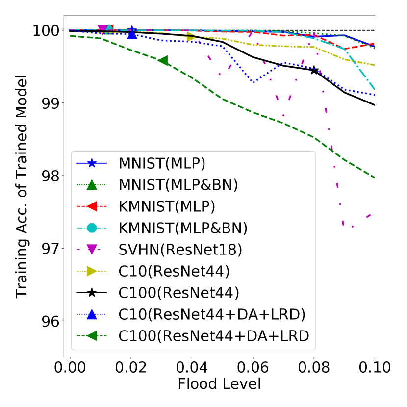
(a) w/o early stopping

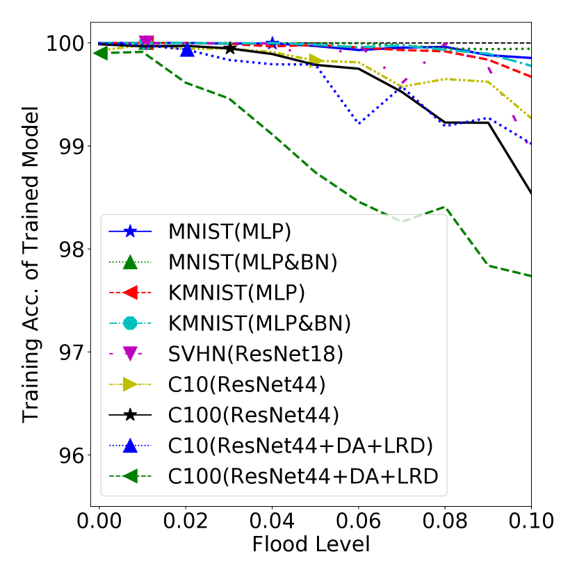
(b) w/ early stopping

Figure 3: Vertical axis is the training accuracy and the horizontal axis is the flood level. Marks are placed on the flood level that was chosen based on validation accuracy.

All datasets and settings show downward curves, implying that the model will give up eventually on memorizing all training data as the flood level becomes higher. A more interesting observation is the position of the optimal flood level (the one chosen by validation accuracy which is marked with $\star$, $\triangle$, $\triangleleft$, $\circ$, $\triangledown$ or $\triangleright$). We can observe that the marks are often plotted at zero error. These results are consistent with recent empirical works that imply zero training error leads to lower generalization error (Belkin et al., 2019; Nakkiran et al., 2020), but we further demonstrate that zero training loss may be harmful under zero training error.

5.2 Performance and gradients

We visualize the relationship between test performance (loss or accuracy) and gradient amplitude of the training/test loss in Fig. 4, where the gradient amplitude is the $\ell_{2}$ norm of the filter-normalized gradient of the loss. The filter-normalized gradient is the gradient appropriately scaled depending on the magnitude of the corresponding convolutional filter, similarly to (Li et al., 2018).

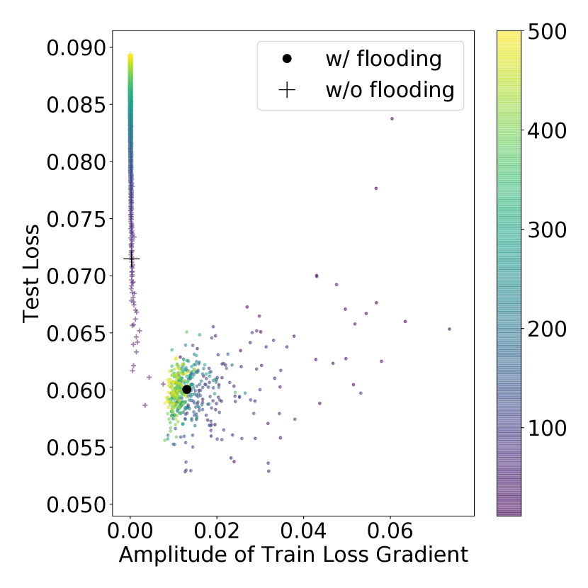
(a) MNIST, x:train

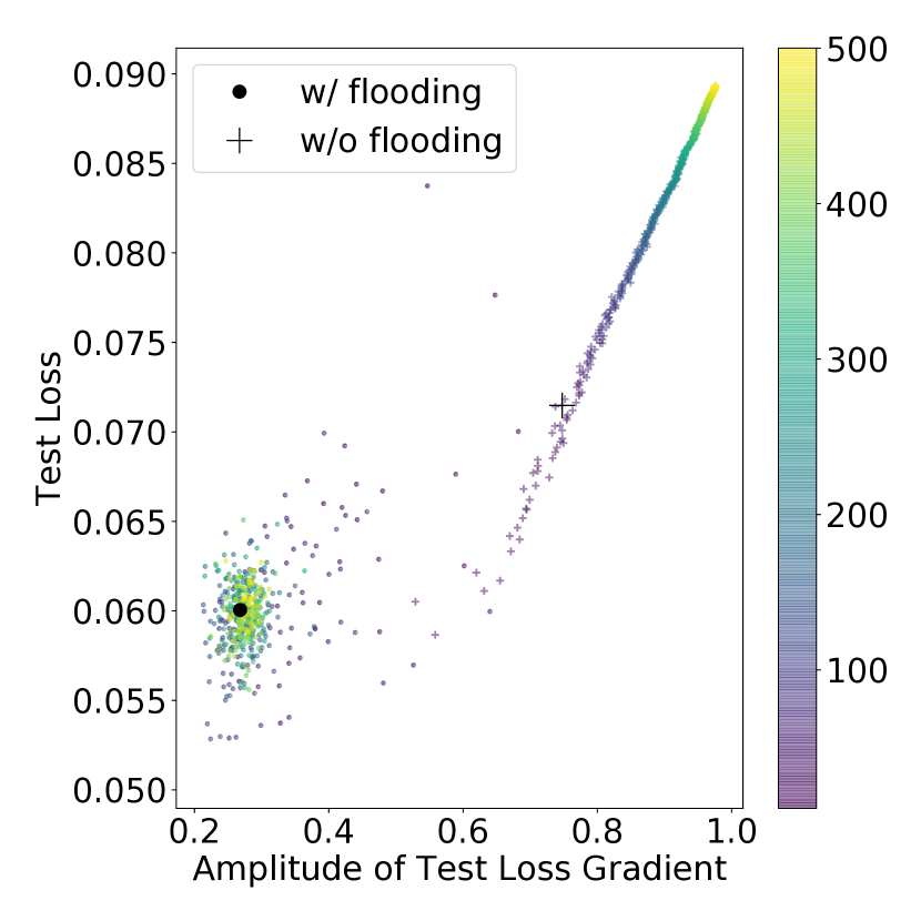
(b) MNIST, x:test

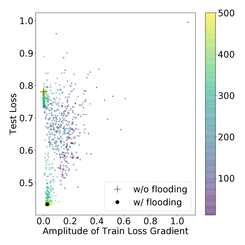
(c) CIFAR-10, x:train

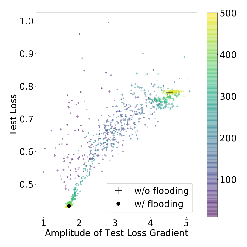
(d) CIFAR-10, x:test

Figure 4: Relationship between test loss and amplitude of gradient (with training or test loss). Each point (“$\circ$” or “$+$”) in the figures corresponds to a single model at a certain epoch. We remove the first 10 epochs and plot the rest. “$\circ$” is used for the method with flooding and “$+$” is used for the method without flooding. The large black “$\circ$” and “$+$” show the epochs with early stopping. The color becomes lighter (purple $\rightarrow$ yellow) as the training proceeds. See Fig. 7 in Appendix for other datasets.

More specifically, for each filter of every convolutional layer, we multiply the corresponding elements of the gradient by the norm of the filter. Note that a fully connected layer is a special case of convolutional layer and is also subject to this scaling.

For the sub-figures with gradient amplitude of training loss on the horizontal axis, “$\circ$” marks (w/ flooding) are often plotted on the right of “$+$” marks (w/o flooding), which implies that flooding prevents the model from staying at a local minimum. For the sub-figures with gradient amplitude of test loss on the horizontal axis, the method with flooding (“$\circ$”) improves performance while the gradient amplitude becomes smaller.

5.3 Flatness

We give a one-dimensional visualization of flatness (Li et al., 2018). We compare the flatness of the model right after the empirical risk with respect to a mini-batch becomes smaller than the flood level, $\widehat{R}_{m}(\bm{g})<b$, for the first time (dotted blue) and the model after training (solid blue). We also compare them with the model trained by the baseline method without flooding, and training is finished (solid red).

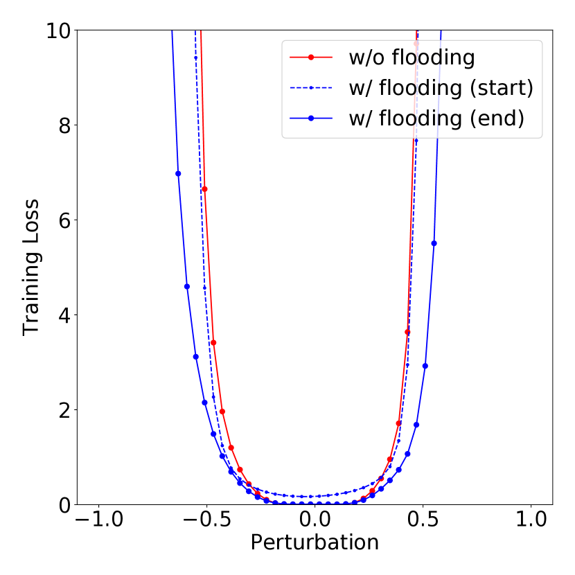
(a) SVHN (train)

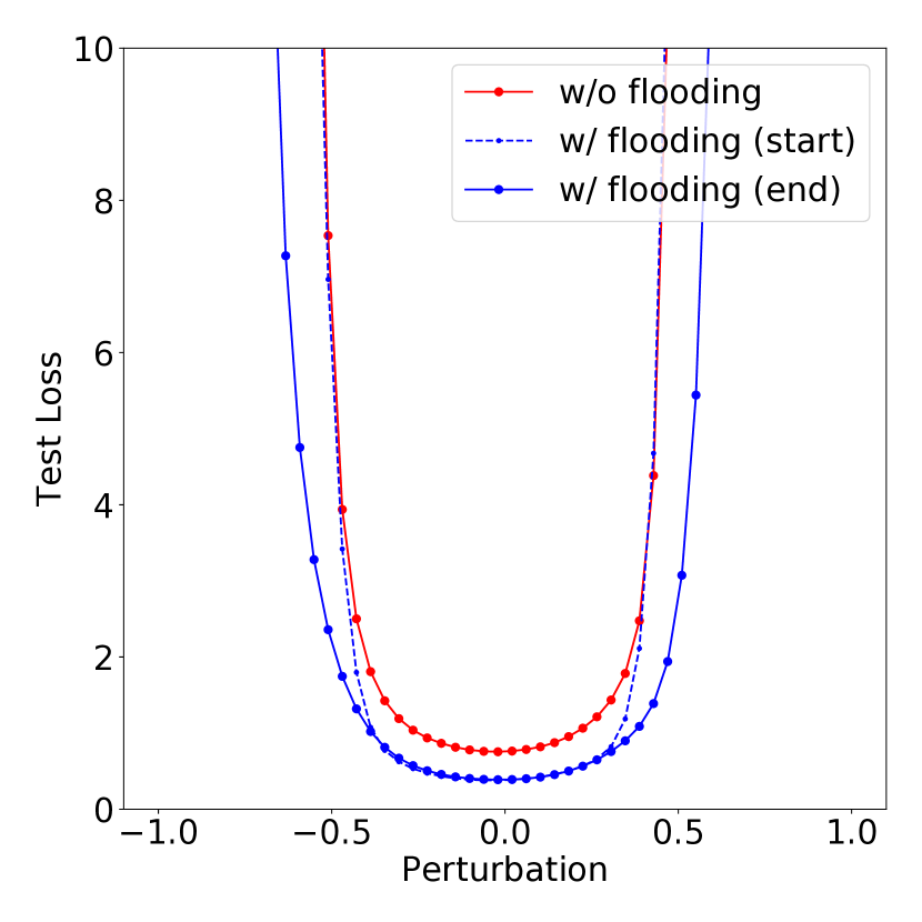
(b) SVHN (test)

(c) CIFAR-10 (train)

(d) CIFAR-10 (test)

Figure 5: One dimensional visualization of flatness of training/test loss with respect to perturbation. We depict the results for 3 models: the model when the empirical risk with respect to training data is below the flooding level for the first time during training(dotted blue), the model at the end of training with flooding (solid blue), and the model at the end of training without flooding (solid red). See Fig. 8 in Appendix for other datasets.

In Fig. 5, the test loss becomes lower and flatter during the training with flooding. Note that the training loss, on the other hand, continues to float around the flood level until the end of training after it enters the flooding zone. We expect that the model makes a random walk and escapes regions with sharp loss landscapes during the period. This may be a possible reason for better generalization results with our proposed method.

5.4 Theoretical Insight

We show that the mean squared error (MSE) of the flooded risk estimator is smaller than that of the original risk estimator without flooding, with the condition that the flood level is between the original training loss and the test loss, in the following theorem.

Theorem 1.

Fix any measurable vector-valued function $\bm{g}$. If the flood level $b$ satisfies $b\leq R(\bm{g})$, we have

$$\mathrm{MSE}(\widehat{R}(\bm{g}))\geq\mathrm{MSE}(\widetilde{R}(\bm{g})).$$ (8)

If $b$ further satisfies $b<R(\bm{g})$ and $\Pr[\widehat{R}(\bm{g})<b]>0$, the inequality will be strict:

$$\mathrm{MSE}(\widehat{R}(\bm{g}))>\mathrm{MSE}(\widetilde{R}(\bm{g})).$$ (9)

See Appendix A for formal discussions and the proof.

6 Conclusion

We proposed a novel regularization method called flooding that keeps the training loss to stay around a small constant value, to avoid zero training loss. In our experiments, the optimal flood level often maintained memorization of training data, with zero error. With flooding, our experiments confirmed that the test accuracy improves for various synthetic and benchmark datasets, and we theoretically showed that the MSE will be reduced under certain conditions.

As a byproduct, we were able to produce a double descent curve for the test loss when flooding was used. An important future direction is to study the relationship between this and the double descent curves from previous works (Krogh & Hertz, 1992; Belkin et al., 2019; Nakkiran et al., 2020).

Appendix A Proof of Theorem 1

Proof.

If the flood level is $b$, then the proposed flooding estimator is

$$\widetilde{R}(\bm{g})=|\widehat{R}(\bm{g})-b|+b.$$ (10)

Since the absolute operator can be expressed with a max operator with $\max(a,b)=\frac{a+b+|a-b|}{2}$, the proposed estimator can be re-expressed as

$$\widetilde{R}(\bm{g})=2\max(\widehat{R}(\bm{g}),b)-\widehat{R}(\bm{g})=A-\widehat{R}(\bm{g}).$$ (11)

For convenience, we used $A=2\max(\widehat{R}(\bm{g}),b)$. From the definition of MSE,

$$\mathrm{MSE}(\widehat{R}(\bm{g}))=\mathbb{E}[(\widehat{R}(\bm{g})-R(\bm{g}))^{2}],$$ (12)

and

$$\mathrm{MSE}(\widetilde{R}(\bm{g})) =\mathbb{E}[(\widetilde{R}(\bm{g})-R(\bm{g}))^{2}]$$ (13)

$$=\mathbb{E}[(A-\widehat{R}(\bm{g})-R(\bm{g}))^{2})]$$ (14)

$$=\mathbb{E}[A^{2}]-2\mathbb{E}[A(\widehat{R}(\bm{g})+R(\bm{g}))]+\mathbb{E}[(\widehat{R}(\bm{g})+R(\bm{g}))^{2}].$$ (15)

We are interested in the sign of

$$\mathrm{MSE}(\widehat{R}(\bm{g}))-\mathrm{MSE}(\widetilde{R}(\bm{g})) =\mathbb{E}[-4\widehat{R}(\bm{g})R(\bm{g})-A^{2}+2A(\widehat{R}(\bm{g})+R(\bm{g}))].$$ (16)

Define the inside of the expectation as $B=-4\widehat{R}(\bm{g})R(\bm{g})-A^{2}+2A(\widehat{R}(\bm{g})+R(\bm{g}))$. $B$ can be divided into two cases, depending on the outcome of the max operator:

$$B= \begin{cases}-4\widehat{R}(\bm{g})R(\bm{g})-4\widehat{R}(\bm{g})^{2}+4\widehat{R}(\bm{g})(\widehat{R}(\bm{g})+R(\bm{g}))\quad&\text{if}\quad\widehat{R}(\bm{g})\geq b\\ -4\widehat{R}(\bm{g})R(\bm{g})-4b^{2}+4b(\widehat{R}(\bm{g})+R(\bm{g}))&\text{if}\quad\widehat{R}(\bm{g})<b\end{cases}$$ (17)

$$= \begin{cases}0\quad&\text{if}\quad\widehat{R}(\bm{g})\geq b\\ -4(b-\widehat{R}(\bm{g}))(b-R(\bm{g}))&\text{if}\quad\widehat{R}(\bm{g})<b.\end{cases}$$ (18)

In the latter case, $B$ becomes positive when $\widehat{R}(\bm{g})<b<R(\bm{g})$.

Therefore, if $b\leq R(\bm{g})$, we have

$$\operatorname{MSE}(\widehat{R}(\bm{g}))-\operatorname{MSE}(\widetilde{R}(\bm{g})) =\mathbb{E}[B\mid\widehat{R}(\bm{g})\geq b]\Pr[\widehat{R}(\bm{g})\geq b]+\mathbb{E}[B\mid\widehat{R}(\bm{g})<b]\Pr[\widehat{R}(\bm{g})<b]$$ (19)

$$=\mathbb{E}[B\mid\widehat{R}(\bm{g})<b]\Pr[\widehat{R}(\bm{g})<b]$$ (20)

$$\geq 0.$$ (21)

Furthermore, if $b<R(\bm{g})$ and $\Pr[\widehat{R}(\bm{g})<b]>0$, we have

$$\operatorname{MSE}(\widehat{R}(\bm{g}))-\operatorname{MSE}(\widetilde{R}(\bm{g}))=\mathbb{E}[B\mid\widehat{R}(\bm{g})<b]\Pr[\widehat{R}(\bm{g})<b]>0.$$ (22)

∎

Appendix B Benchmark Datasets

In the experiments in Section 4.2, we use 6 image benchmark datasets explained below.

• MNIST (Lecun et al., 1998) is a 10 class dataset of handwritten digits: $1,2\ldots,9$ and $0$. Each sample is a $28\times 28$ grayscale image. The number of training and test samples are 60,000 and 10,000, respectively.

• Kuzushiji-MNIST (Clanuwat et al., 2018) is a 10 class dataset of cursive Japanese (“Kuzushiji”) characters. Each sample is a $28\times 28$ grayscale image. The number of training and test samples are 60,000 and 10,000, respectively.

• SVHN (Netzer et al., 2011) is a 10 class dataset of house numbers from Google Street View images, in $32\times 32\times 3$ RGB format. 73257 digits are for training and 26032 digits are for testing.

• CIFAR-10 is a 10 class dataset of various objects: airplane, automobile, bird, cat, deer, dog, frog, horse, ship, and truck. Each sample is a colored image in $32\times 32\times 3$ RGB format. It is a subset of the 80 million tiny images dataset (Torralba et al., 2008). There are 6,000 images per class, where 5,000 are for training and 1,000 are for test.

• CIFAR-100 is a 100 class dataset of various objects. Each class has 600 samples, where 500 samples are for training and 100 samples are for test. This is also a subset of the 80 million tiny images dataset (Torralba et al., 2008).

Appendix C Learning Curves

In Fig. 6, we show more results of learning curves of the test loss. Note that Figure 1(c) shows the learning curves for the first 80 epochs for CIFAR-10 without flooding with ResNet-18. Figure 1(d) shows the learning curves with flooding, when the flood level is $0.18$ also with ResNet-18. Other details follow the experiments in Section 4.2.

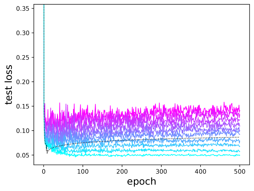
(a) MNIST, MLP

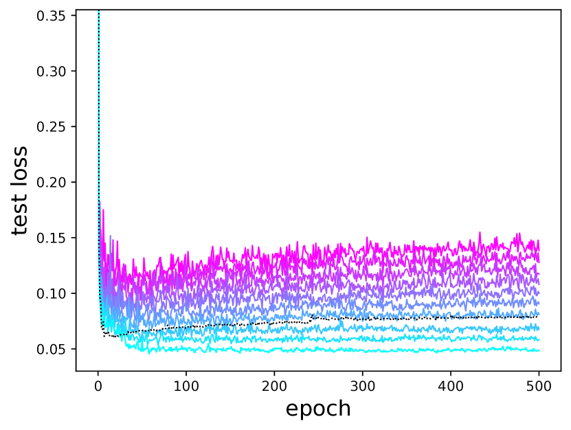
(b) MNIST, MLP&BN

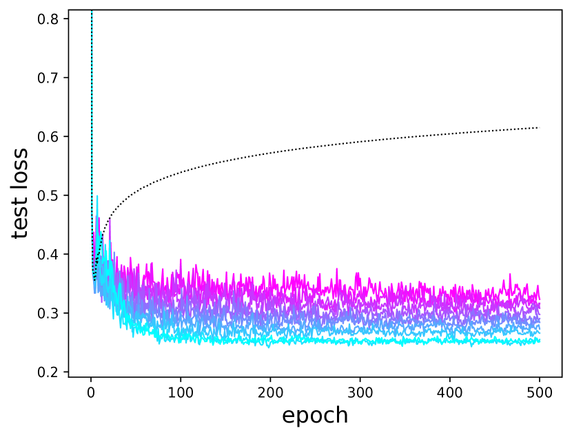
(c) KMNIST, MLP

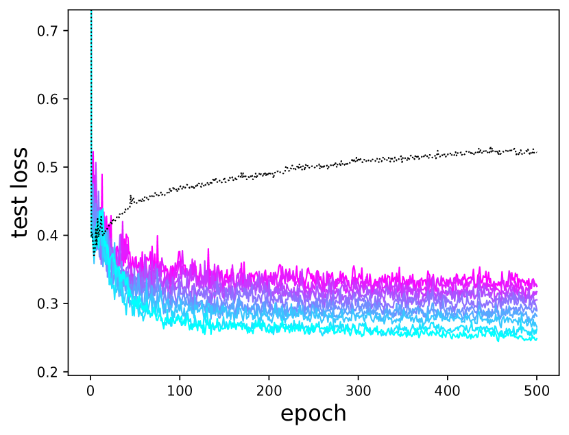
(d) KMNIST, MLP&BN

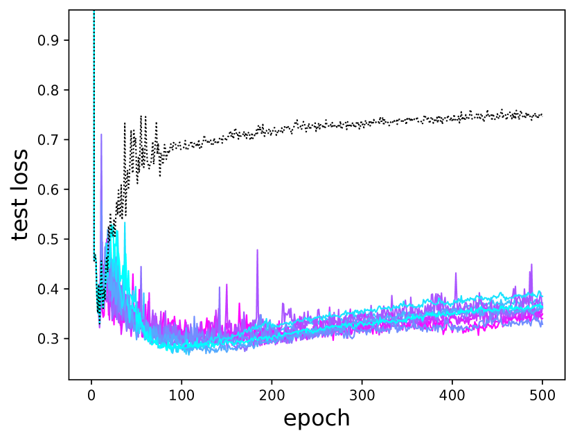
(e) SVHN, ResNet18

(f) C10, ResNet44

(g) C10, ResNet44, DA & LRD

(h) C100, ResNet44

(i) C100, ResNet44, DA & LRD

Figure 6: Learning curves of the test loss showing that adding flooding leads to lower test loss. The black dotted line shows the baseline without flooding. The colored lines show the learning curves with flooding for different flooding levels. We show the learning curves for $b\in\{0.01,0.02,\ldots,0.10\}$. KMNIST is Kuzushiji-MNIST, C10 is CIFAR-10, and C100 is CIFAR-100. MLP, BN, DA, and LRD stand for multi-layer perceptron, batch normalization, data augmentation and learning rate decay, respectively.

Appendix D Additional Figures for Section 5.2 and Section 5.3

See Fig. 7 and Fig. 8 for datasets that were not included in the main paper.

(a) MNIST, x:train

(b) MNIST, x:test

(c) KMNIST, x:train

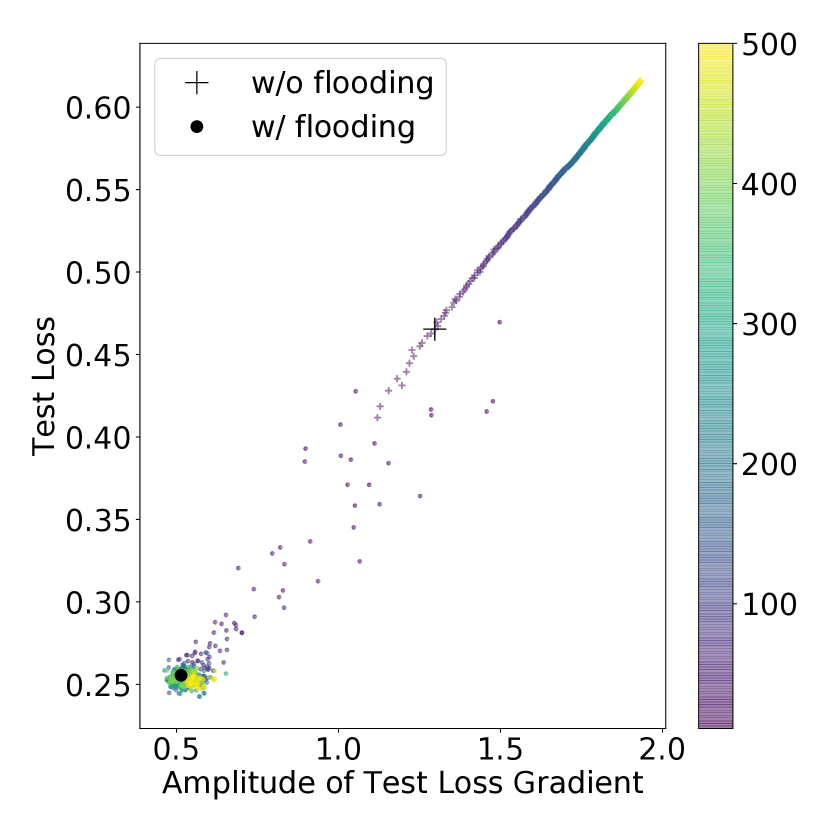
(d) KMNIST, x:test

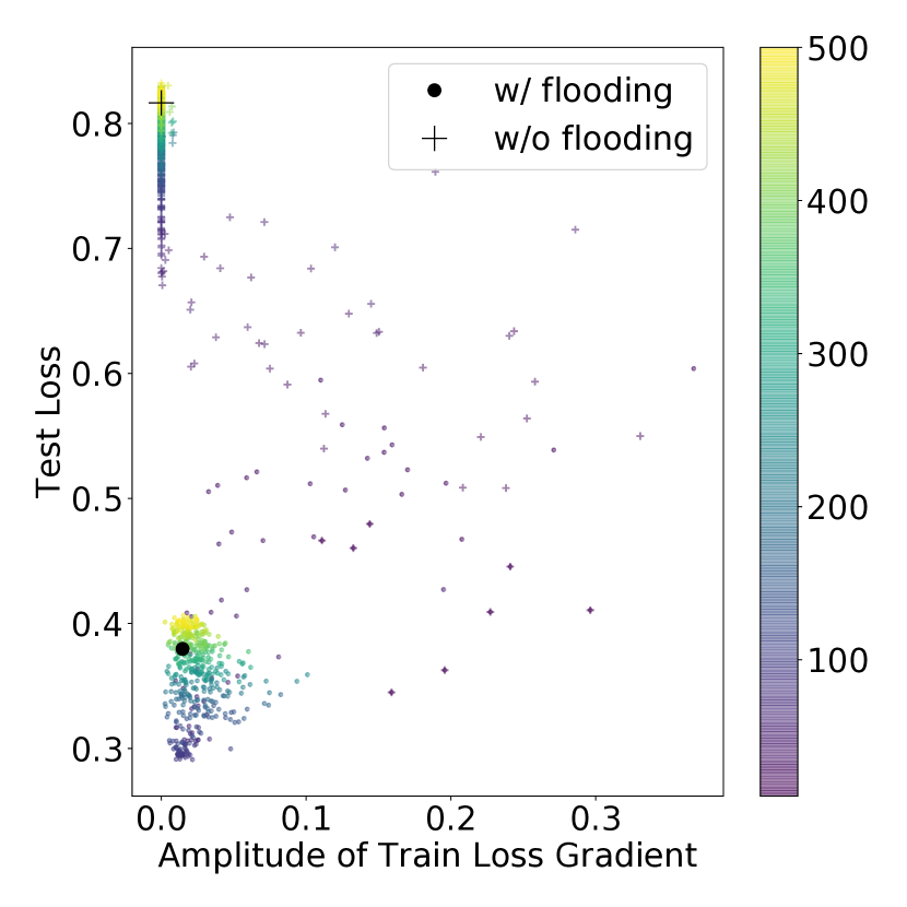
(e) SVHN, x:train

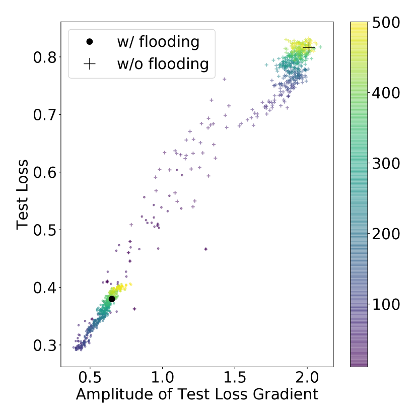
(f) SVHN, x:test

(g) CIFAR-10, x:train

(h) CIFAR-10, x:test

(i) CIFAR-100, x:train

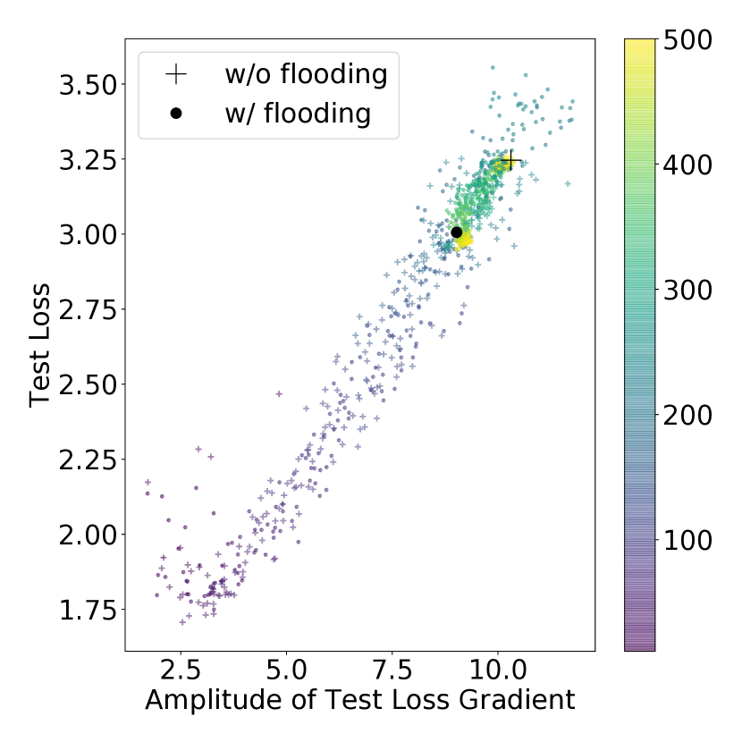
(j) CIFAR-100, x:test

Figure 7: Relationship between test loss and amplitude of gradient (with training or test loss). Each point (“$\circ$” or “$+$”) in the figures corresponds to a single model at a certain epoch. We remove the first 10 epochs and plot the rest. “$\circ$” is used for the method with flooding and “$+$” is used for the method without flooding. The large black “$\circ$” and “$+$” show the epochs with early stopping. The color becomes lighter (purple $\rightarrow$ yellow) as the training proceeds.

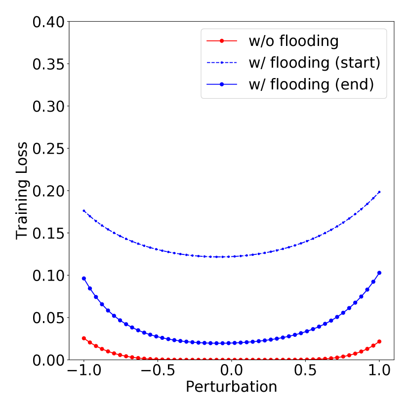
(a) MNIST (train)

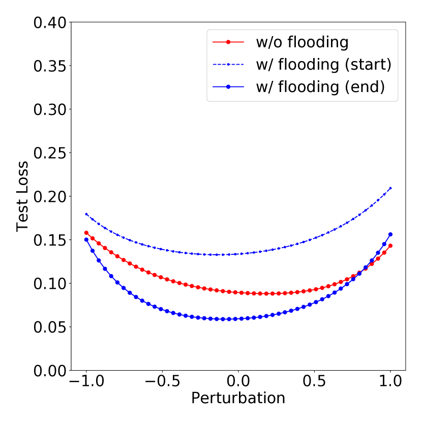
(b) MNIST (test)

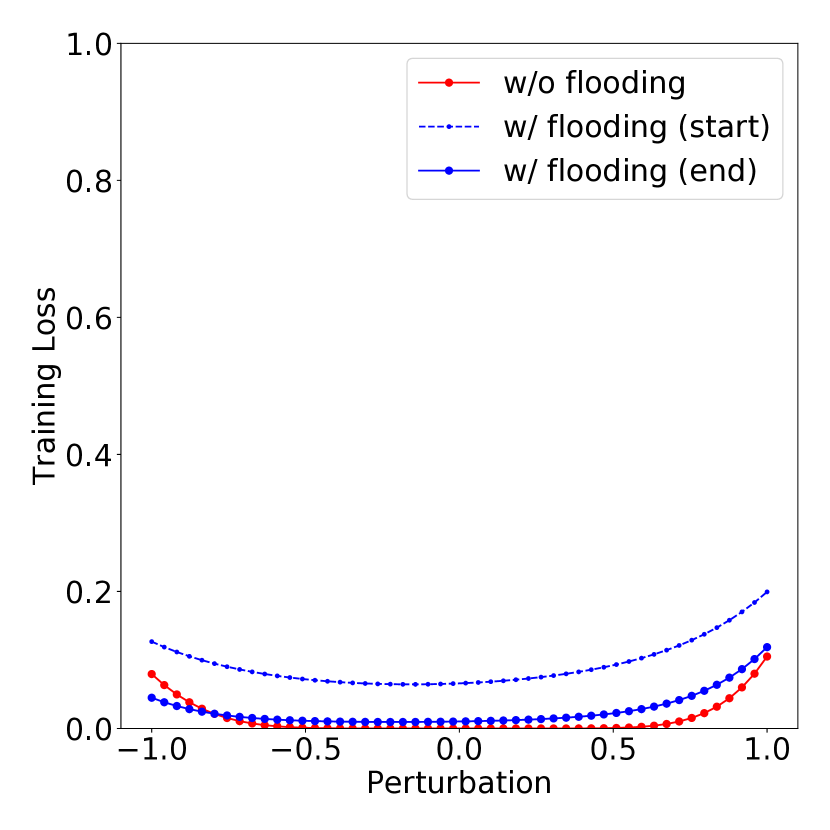
(c) KMNIST (train)

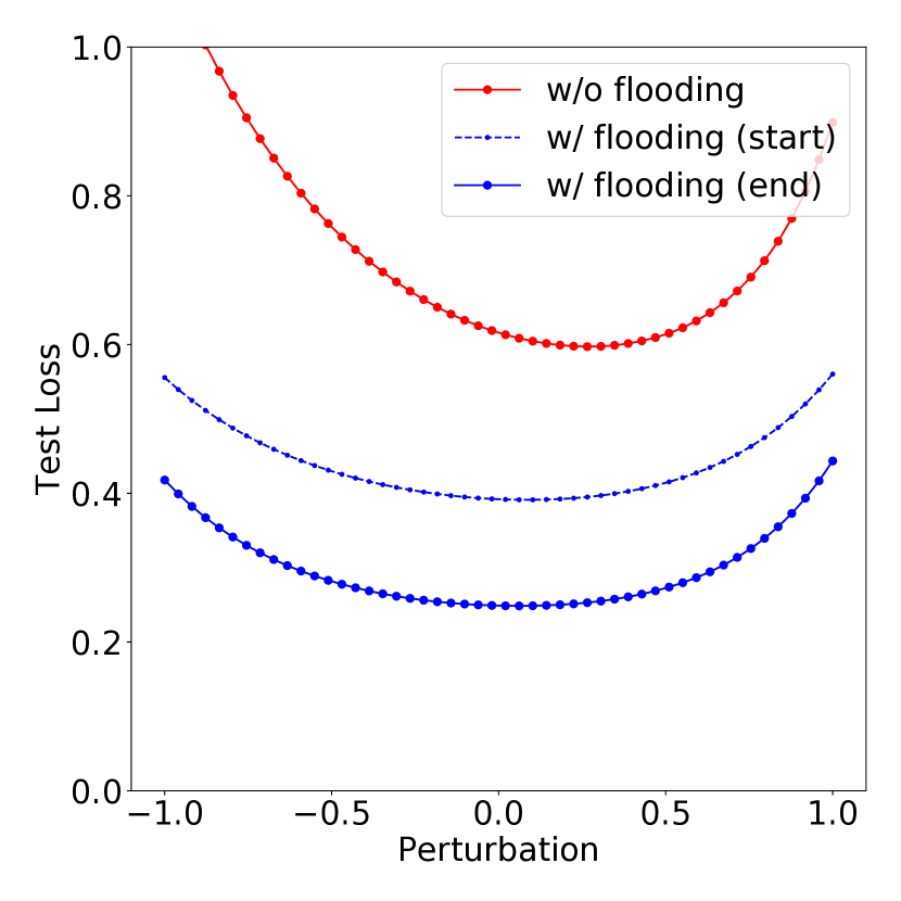
(d) KMNIST (test)

(e) SVHN (train)

(f) SVHN (test)

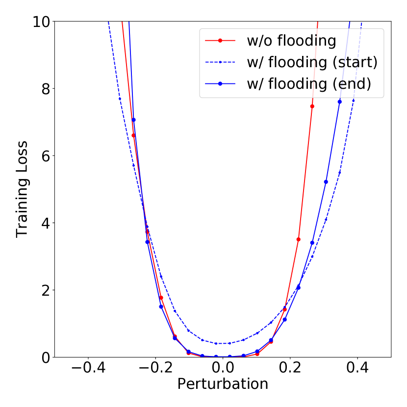
(g) CIFAR-10 (train)

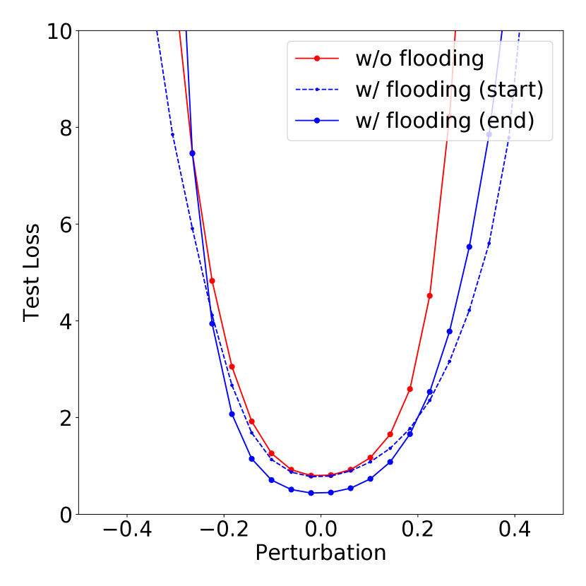
(h) CIFAR-10 (test)

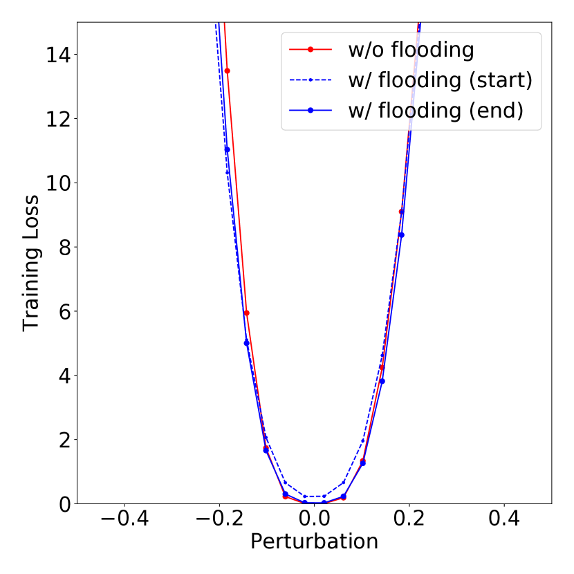
(i) CIFAR-100 (train)

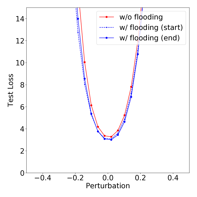
(j) CIFAR-100 (test)

Figure 8: One-dimensional visualization of flatness. We visualize the training/test loss with respect to perturbation. We depict the results for 3 models: the model when the empirical risk with respect to training data is below the flooding level for the first time during training (dotted blue), the model at the end of training with flooding (solid blue), and the model at the end of training without flooding (solid red).

References

- Arpit et al. (2017) Arpit, D., Jastrzebski, S., Ballas, N., Krueger, D., Bengio, E., Kanwal, M. S., Maharaj, T., Fischer, A., Courville, A., Bengio, Y., and Lacoste-Julien, S. A closer look at memorization in deep networks. In ICML, 2017.
- Belkin et al. (2018) Belkin, M., Hsu, D. J., and Mitra, P. Overfitting or perfect fitting? Risk bounds for classification and regression rules that interpolate. In NeurIPS, 2018.
- Belkin et al. (2019) Belkin, M., Hsu, D., Ma, S., and Mandal, S. Reconciling modern machine-learning practice and the classical bias–variance trade-off. PNAS, 116:15850–15854, 2019.
- Berthelot et al. (2019) Berthelot, D., Carlini, N., Goodfellow, I., Papernot, N., Oliver, A., and Raffel, C. A. MixMatch: A holistic approach to semi-supervised learning. In NeurIPS, 2019.
- Bishop (1995) Bishop, C. M. Regularization and complexity control in feed-forward networks. In ICANN, 1995.
- Bishop (2011) Bishop, C. M. Pattern Recognition and Machine Learning (Information Science and Statistics). Springer, 2011.
- Caruana et al. (2000) Caruana, R., Lawrence, S., and Giles, C. L. Overfitting in neural nets: Backpropagation, conjugate gradient, and early stopping. In NeurIPS, 2000.
- Chaudhari et al. (2017) Chaudhari, P., Choromanska, A., Soatto, S., LeCun, Y., Baldassi, C., Borgs, C., Chayes, J., Sagun, L., and Zecchina, R. Entropy-SGD: Biasing gradient descent into wide valleys. In ICLR, 2017.
- Cid-Sueiro et al. (2014) Cid-Sueiro, J., García-García, D., and Santos-Rodríguez, R. Consistency of losses for learning from weak labels. In ECML-PKDD, 2014.
- Clanuwat et al. (2018) Clanuwat, T., Bober-Irizar, M., Kitamoto, A., Lamb, A., Yamamoto, K., and Ha, D. Deep learning for classical Japanese literature. In NeurIPS Workshop on Machine Learning for Creativity and Design, 2018.
- du Plessis et al. (2014) du Plessis, M. C., Niu, G., and Sugiyama, M. Analysis of learning from positive and unlabeled data. In NeurIPS, 2014.
- du Plessis et al. (2015) du Plessis, M. C., Niu, G., and Sugiyama, M. Convex formulation for learning from positive and unlabeled data. In ICML, 2015.
- Goodfellow et al. (2016) Goodfellow, I., Bengio, Y., and Courville, A. Deep Learning. MIT Press, 2016.
- Guo et al. (2017) Guo, C., Pleiss, G., Sun, Y., and Weinberger, K. Q. On calibration of modern neural networks. In ICML, 2017.
- Guo et al. (2019) Guo, H., Mao, Y., and Zhang, R. Augmenting data with mixup for sentence classification: An empirical study. In arXiv:1905.08941, 2019.
- Han et al. (2020) Han, B., Niu, G., Yu, X., Yao, Q., Xu, M., Tsang, I. W., and Sugiyama, M. Sigua: Forgetting may make learning with noisy labels more robust. In ICML, 2020.
- Hanson & Pratt (1988) Hanson, S. J. and Pratt, L. Y. Comparing biases for minimal network construction with back-propagation. In NeurIPS, 1988.
- He et al. (2016) He, K., Zhang, X., Ren, S., and Sun, J. Deep residual learning for image recognition. In CVPR, 2016.
- Hochreiter & Schmidhuber (1997) Hochreiter, S. and Schmidhuber, J. Flat minima. Neural Computation, 9:1–42, 1997.
- Idelbayev (2020) Idelbayev, Y. Proper ResNet implementation for CIFAR10/CIFAR100 in PyTorch. https//github.com/akamaster/pytorch_resnet_cifar10, 2020. Accessed: 2020-05-31.
- Ioffe & Szegedy (2015) Ioffe, S. and Szegedy, C. Batch normalization: Accelerating deep network training by reducing internal covariate shift. In ICML, 2015.
- Ishida et al. (2019) Ishida, T., Niu, G., Menon, A. K., and Sugiyama, M. Complementary-label learning for arbitrary losses and models. In ICML, 2019.
- Keskar et al. (2017) Keskar, N. S., Mudigere, D., Nocedal, J., Smelyanskiy, M., and Tang, P. T. P. On large-batch training for deep learning: Generalization gap and sharp minima. In ICLR, 2017.
- Kingma & Ba (2015) Kingma, D. P. and Ba, J. L. Adam: A method for stochastic optimization. In ICLR, 2015.
- Kiryo et al. (2017) Kiryo, R., Niu, G., du Plessis, M. C., and Sugiyama, M. Positive-unlabeled learning with non-negative risk estimator. In NeurIPS, 2017.
- Kolesnikov et al. (2020) Kolesnikov, A., Beyer, L., Zhai, X., Puigcerver, J., Yung, J., Gelly, S., and Houlsby, N. Big transfer (BiT): General visual representation learning. In arXiv:1912.11370v3, 2020.
- Krogh & Hertz (1992) Krogh, A. and Hertz, J. A. A simple weight decay can improve generalization. In NeurIPS, 1992.
- Lecun et al. (1998) Lecun, Y., Bottou, L., Bengio, Y., and Haffner, P. Gradient-based learning applied to document recognition. In Proceedings of the IEEE, pp. 2278–2324, 1998.
- Li et al. (2018) Li, H., Xu, Z., Taylor, G., Studer, C., and Goldstein, T. Visualizing the loss landscape of neural nets. In NeurIPS, 2018.
- Loshchilov & Hutter (2019) Loshchilov, I. and Hutter, F. Decoupled weight decay regularization. In ICLR, 2019.
- Lu et al. (2020) Lu, N., Zhang, T., Niu, G., and Sugiyama, M. Mitigating overfitting in supervised classification from two unlabeled datasets: A consistent risk correction approach. In AISTATS, 2020.
- Morgan & Bourlard (1990) Morgan, N. and Bourlard, H. Generalization and parameter estimation in feedforward nets: Some experiments. In NeurIPS, 1990.
- Nair & Hinton (2010) Nair, V. and Hinton, G. Rectified linear units improve restricted boltzmann machines. In ICML, 2010.
- Nakkiran et al. (2019) Nakkiran, P., Kaplun, G., Kalimeris, D., Yang, T., Edelman, B. L., Zhang, F., and Barak, B. SGD on neural networks learns functions of increasing complexity. In NeurIPS, 2019.
- Nakkiran et al. (2020) Nakkiran, P., Kaplun, G., Bansal, Y., Yang, T., Barak, B., and Sutskever, I. Deep double descent: Where bigger models and more data hurt. In ICLR, 2020.
- Natarajan et al. (2013) Natarajan, N., Dhillon, I. S., Ravikumar, P. K., and Tewari, A. Learning with noisy labels. In NeurIPS, 2013.
- Netzer et al. (2011) Netzer, Y., Wang, T., Coates, A., Bissacco, A., Wu, B., and Ng, A. Y. Reading digits in natural images with unsupervised feature learning. In NeurIPS Workshop on Deep Learning and Unsupervised Feature Learning, 2011.
- Ng (1997) Ng, A. Y. Preventing “overfitting” of cross-validation data. In ICML, 1997.
- Paszke et al. (2019) Paszke, A., Gross, S., Massa, F., Lerer, A., Bradbury, J., Chanan, G., Killeen, T., Lin, Z., Gimelshein, N., Antiga, L., Desmaison, A., Kopf, A., Yang, E., DeVito, Z., Raison, M., Tejani, A., Chilamkurthy, S., Steiner, B., Fang, L., Bai, J., and Chintala, S. PyTorch: An imperative style, high-performance deep learning library. In NeurIPS, 2019.
- Patrini et al. (2017) Patrini, G., Rozza, A., Menon, A. K., Nock, R., and Qu, L. Making deep neural networks robust to label noise: A loss correction approach. In CVPR, 2017.
- Robbins & Monro (1951) Robbins, H. and Monro, S. A stochastic approximation method. Annals of Mathematical Statistics, 22:400–407, 1951.
- Roelofs et al. (2019) Roelofs, R., Shankar, V., Recht, B., Fridovich-Keil, S., Hardt, M., Miller, J., and Schmidt, L. A meta-analysis of overfitting in machine learning. In NeurIPS, 2019.
- Shorten & Khoshgoftaar (2019) Shorten, C. and Khoshgoftaar, T. M. A survey on image data augmentation for deep learning. Journal of Big Data, 6, 2019.
- Srivastava et al. (2014) Srivastava, N., Hinton, G., Krizhevsky, A., Sutskever, I., and Salakhutdinov, R. Dropout: A simple way to prevent neural networks from overfitting. Journal of Machine Learning Research, 15:1929–1958, 2014.
- Sugiyama (2015) Sugiyama, M. Introduction to statistical machine learning. Morgan Kaufmann, 2015.
- Szegedy et al. (2016) Szegedy, C., Vanhoucke, V., Ioffe, S., and Shlens, J. Rethinking the inception architecture for computer vision. In CVPR, 2016.
- Thulasidasan et al. (2019) Thulasidasan, S., Chennupati, G., Bilmes, J., Bhattacharya, T., and Michalak, S. On mixup training: Improved calibration and predictive uncertainty for deep neural networks. In NeurIPS, 2019.
- Tibshirani (1996) Tibshirani, R. Regression shrinkage and selection via the lasso. Journal of the Royal Statistical Society: Series B (Methodological), 58:267–288, 1996.
- Tikhonov (1943) Tikhonov, A. N. On the stability of inverse problems. Doklady Akademii Nauk SSSR, 39:195–198, 1943.
- Tikhonov & Arsenin (1977) Tikhonov, A. N. and Arsenin, V. Y. Solutions of Ill Posed Problems. Winston, 1977.
- Torralba et al. (2008) Torralba, A., Fergus, R., and Freeman, W. T. 80 million tiny images: A large data set for nonparametric object and scene recognition. In IEEE Trans. PAMI, 2008.
- van Rooyen & Williamson (2018) van Rooyen, B. and Williamson, R. C. A theory of learning with corrupted labels. Journal of Machine Learning Research, 18:1–50, 2018.
- Verma et al. (2019) Verma, V., Lamb, A., Kannala, J., Bengio, Y., and Lopez-Paz, D. Interpolation consistency training for semi-supervised learning. In IJCAI, 2019.
- Wager et al. (2013) Wager, S., Wang, S., and Liang, P. Dropout training as adaptive regularization. In NeurIPS, 2013.
- Werpachowski et al. (2019) Werpachowski, R., György, A., and Szepesvári, C. Detecting overfitting via adversarial examples. In NeurIPS, 2019.
- Zhang et al. (2017) Zhang, C., Bengio, S., Hardt, M., Recht, B., and Vinyals, O. Understanding deep learning requires rethinking generalization. In ICLR, 2017.
- Zhang et al. (2018) Zhang, H., Cisse, M., Dauphin, Y. N., and Lopez-Paz, D. mixup: Beyond empirical risk minimization. In ICLR, 2018.
- Zhang (2004) Zhang, T. Statistical behavior and consistency of classification methods based on convex risk minimization. The Annals of Statistics, 32:56–85, 2004.