Stochastic Optimization for
Regularized Wasserstein Estimators

Abstract

Optimal transport is a foundational problem in optimization, that allows to compare probability distributions while taking into account geometric aspects. Its optimal objective value, the Wasserstein distance, provides an important loss between distributions that has been used in many applications throughout machine learning and statistics. Recent algorithmic progress on this problem and its regularized versions have made these tools increasingly popular. However, existing techniques require solving an optimization problem to obtain a single gradient of the loss, thus slowing down first-order methods to minimize the sum of losses, that require many such gradient computations. In this work, we introduce an algorithm to solve a regularized version of this problem of Wasserstein estimators, with a time per step which is sublinear in the natural dimensions of the problem. We introduce a dual formulation, and optimize it with stochastic gradient steps that can be computed directly from samples, without solving additional optimization problems at each step. Doing so, the estimation and computation tasks are performed jointly. We show that this algorithm can be extended to other tasks, including estimation of Wasserstein barycenters. We provide theoretical guarantees and illustrate the performance of our algorithm with experiments on synthetic data.

1 Introduction

Optimal transport is one of the foundational problems of optimisation (Monge, 1781; Kantorovich, 2006), and an important topic in analysis (Villani, 2008). It asks how one can transport mass with distribution measure $\mu$ to another distribution measure $\nu$, with minimal global transport cost. It can also be written with a probabilistic interpretation, known as the Monge-Kantorovich formulation, of finding a joint distribution $\pi$ in the set $\Pi(\mu,\nu)$ of those with marginals $\mu$ and $\nu$, minimizing an expected cost between variables $X$ and $Y$. The minimum value gives rise to a natural statistical tool to compare distributions, known as the Wasserstein (or earth-mover’s) distance,

$$W_{c}(\mu,\nu)=\operatorname{OT}(\mu,\nu)=\min_{\pi\in\Pi(\mu,\nu)}\mathbb{E}_{(X,Y)\sim\pi}\left[c(X,Y)\right].$$

In the case of finitely supported measures, taken with same support size $n$ for ease of notation, such as two empirical measures from samples, it is written as a linear program (on the right). It can be solved by the Hungarian algorithm (Kuhn, 1955), which runs in time $O(n^{3})$. While tractable, this is still relatively expensive for extremely large-scale applications in modern machine learning, where one hopes for running times that are linear in the size of the input (here $n^{2}$).

Attention to this problem has been recently renewed in machine learning, in particular due to recent advances to efficiently solve an entropic-regularized version (Cuturi, 2013), and its uses in many applications (see e.g. Peyré et al., 2019, for a survey), as it allows to capture the geometric aspects of the data. This problem has a strongly convex objective, and its solution converges to that of the optimal transport problem whenthe regularization parameter goes to 0. It can be easily solved with the Sinkhorn algorithm (Sinkhorn, 1964; Altschuler et al., 2017), or by other methods in time $O(n^{2}\log n)$ (Dvurechensky et al., 2018).

These tools have been applied in a wide variety of fields, from machine learning (Alvarez-Melis et al., 2018; Arjovsky et al., 2017; Gordaliza et al., 2019; Flamary et al., 2018), natural language processing (Grave et al., 2019; Alaux et al., 2019; Alvarez-Melis et al., 2018), computer graphics (Feydy et al., 2017; Lavenant et al., 2018; Solomon et al., 2015), the natural sciences (del Barrio et al., 2019; Schiebinger et al., 2019), and learning under privacy (Boursier and Perchet, 2019).

Of particular interests to statistics and machine learning are analyses of this problem with only sample access to the distributions. There have been growing efforts to estimate either the objective value of this problem, or the unknown distribution, with this metric or associated regularized metrics (see below) (Weed et al., 2019; Genevay et al., 2019; Uppal et al., 2019). One of the motivations are variational Wasserstein problems, where the objective value of an optimal transport problem is used as a loss, and one seeks to minimize in a parameter $\theta$ an objective that depends on a known distribution $\nu_{\theta}$

$$\min_{\theta\in\Theta}\operatorname{OT}(\nu_{\theta},\mu)\,,$$

where $\mu$ is only accessible through samples. This method for estimation, referred to as minimum Kantorovich estimators (Bassetti et al., 2006), mirrors the interpretation of likelihood maximization as the minimization of $\operatorname{KL}(\nu_{\theta},\mu)$, with the Kullback-Leibler divergence.

The value of the entropic-regularized problem, or of the related Sinkhorn divergence, can also be used as a loss in learning tasks (Alvarez-Melis et al., 2018; Genevay et al., 2017; Luise et al., 2018), and compared to other metrics such as maximum mean discrepency (Gretton et al., 2012; Feydy et al., 2019; Arbel et al., 2019). One of the advantages of the regularized problem is the existence of gradients in the parameters of the problem (cost matrix, target measures).

The problem of minimizing this loss for the $\ell_{2}$ cost over $\mathbb{R}^{d}$ has been shown to be equivalent to maximum likelihood Gaussian deconvolution (Rigollet and Weed, 2018). We show here that this result can be generalized for all cost functions to maximum likelihood estimation for a kernel inversion problem. It is not only the solution of a stochastic optimization problem, but also an estimator, referred to here as the regularized Wasserstein estimator.

In this work, we propose a new stochastic optimization scheme to minimize the $\operatorname{OT}_{\varepsilon}$ between an unknown discrete measure $\mu$ and another discrete measure $\nu\in\mathcal{M}$, with an additional regularization term on $\nu$. There are many connections between this problem and stochastic optimization: by a dual formulation, the value $\operatorname{OT}_{\varepsilon}(\mu,\nu)$ can be written as the optimum of an expectation in $\mu,\nu$, allowing simple computations with only sample access (Genevay et al., 2016). Here, we take this one step further and design an algorithm to optimize in $\nu$, not just evaluate this loss. A direct approach is to optimize by first-order methods, by the use of stochastic gradients in $\nu$ at each step (Genevay et al., 2017). However, these gradient estimates are based on dual solutions of the regularized problem, so obtaining them requires to solve an optimization problem, with running time scaling quadratically in the intrinsic dimension of the problem (the size of the supports of $\mu,\nu$). For the dual formulation that we introduce, stochastic gradients can be directly computed from samples. Algorithmic techniques exploiting the particular structure of the dual formulation for this regularization allow us to compute these gradients in constant time. We follow here the recent developments in sublinear algorithms based on stochastic methods (Clarkson et al., 2012).

We provide theoretical guarantees on the convergence of the final iterate $\nu_{t}$ to the true minimizer $\nu^{*}$, and demonstrate these results on simulated experiments.

2 Problem Description

Definitions.

Let $\mu$ be a probability measure on $\mathbb{R}^{d}$ with finite support $\mathcal{X}=\{x_{i}\}_{1\leq i\leq I}\subset\mathbb{R}^{d}$ and a family $\mathcal{M}$ of probability measures. The measures in $\mathcal{M}$ should all be absolutely continuous with respect to a known measure $\beta$ supported in the finite set $\mathcal{Y}=\{y_{j}\}_{1\leq j\leq J}\subset\mathbb{R}^{d}$. We consider the following minimization problem:

$$\min_{\nu\in\mathcal{M}}\operatorname{OT}_{\varepsilon}(\mu,\nu)+\eta\operatorname{KL}(\nu,\beta).$$ (1)

In this expression, $\operatorname{OT}_{\varepsilon}$ is the regularised optimal transport cost defined by the following expression

$$\operatorname{OT}_{\varepsilon}(\mu,\nu)=\min_{\pi\in\Pi(\mu,\nu)}\mathbb{E}_{(X,Y)\sim\pi}\left[c(X,Y)\right]+\varepsilon\operatorname{KL}(\pi,\mu\otimes\nu),$$ (2)

where the minimum is taken over the set

$$\Pi(\mu,\nu)=\left\{\pi\in\mathcal{P}(X\times Y):\pi_{X}=\mu,\ \pi_{Y}=\nu\right\}$$

of couplings of $\mu$ and $\nu$, and $c$ is a cost function in $\mathbb{R}^{d}$. The operator $\operatorname{KL}(\cdot,\cdot)$ is the Kullback-Leibler divergence, defined as

$$\operatorname{KL}(\mu_{1},\mu_{2})=\mathbb{E}_{Z\sim\mu_{2}}\left[\frac{d\mu_{1}}{d\mu_{2}}(Z)\log\left(\frac{d\mu_{1}}{d\mu_{2}}(Z)\right)\right],$$

for two measures $\mu_{1}$ and $\mu_{2}$ such that $\mu_{1}\ll\mu_{2}$. We assume that $\mathcal{M}$ is convex for the problem to be a convex optimization problem, and compact to guarantee that the minimum is attained.

Remark 1.

If $c$ is a distance and if $\varepsilon=\eta=0$, then $\operatorname{OT}_{\varepsilon}$ is a Wasserstein distance and our problem can be seen as computing a projection of $\mu$ onto $\mathcal{M}$. In the discrete case, the solution to the unregularized problem is the distribution $\nu$ such that $\nu(y)=\mu(x)$, where $y$ is the nearest neighbour in $\mathcal{Y}$ of $x$.

Learning problem.

Our objective is to solve the optimization problem in Equation (1), given observations $X_{i}$ independent and identically distributed (i.i.d.) from $\mu$ that is unknown, and sample access to $\beta$. These can be assumed to be simulated by the user if $\beta$ is known, as part of the regularization. This problem can be either be interpreted as an unsupervised learning problem or as estimation in an inverse problem, and we refer to it as regularized Wasserstein estimation. The term in Kullback-Leibler (or entropy, up to an offset) are classical manners in which a probability can be regularized.

Maximum likelihood interpretation.

While the unregularized problem has a trivial solution, there is in general no closed form for positive $\varepsilon$. When $\varepsilon>0$, $\eta=0$ and $\mathcal{M}$ is the set of all probability measures on $Y$, then our problem is equivalent to the maximum likelihood estimator for a kernel inversion problem. This corresponds to estimating the unknown initial distribution of a random variable $Y$, but only by observing it after the action of a specific transition kernel $\kappa$ (see, e.g., Berthet and Kanade, 2019, for the statistical complexity of estimating initial dustributions under general Markov kernels).

Proposition 2.1 (MLE interpretation).

Let $\mathcal{M}$ be the set of all probability measures on $Y$, let $\nu^{*}$ be a measure on $Y$, and let $\kappa:Y\to X$ be a transition kernel of the form

$$\kappa(x,y)=\frac{\exp{\left(-\frac{c(x,y)}{\varepsilon}\right)}}{\sum_{x^{\prime}\in X}\exp{\left(-\frac{c(x^{\prime},y)}{\varepsilon}\right)}},$$

the observed measure is $\mu=\kappa\nu^{*}$, which can be written as

$$\mu(x)=\int_{Y}\kappa(x,y)d\nu^{*}(y).$$

The maximum likelihood estimation of $\nu^{*}$ for this observation is

$$\hat{\nu}:=\arg\max_{\nu\in\mathcal{M}}\sum_{i}\log(\kappa\nu)(X_{i}).$$

This estimator also verifies

$$\hat{\nu}=\arg\min_{\nu\in\mathcal{M}}\operatorname{OT}_{\varepsilon}(\mu,\nu).$$ (3)

Remark 2.

If $c(x,y)=\|x-y\|^{2}$, then $\kappa(x,y)=:\phi_{\varepsilon}(x-y)$ is a Gaussian convolution kernel and the sample measure $\mu=\phi\star\nu^{*}$ is a convolution, so the solution of (3) is the MLE of the Gaussian deconvolution problem, as already presented by Rigollet and Weed (2018).

As in the Gaussian case, these optimization problems share an optimum, but are not equal in value. Therefore, in our regularized setting, it is not possible to substitute one for the other.

3 Dual formulations

As noted above, first-order optimization methods to solve directly in $\nu$ the regularized problem require at every step to solve an optimization problem. We explore instead another approach, through a dual formulation of our problem. Such a formulation allows to change the minimisation problem in (2) into a maximisation problem.

Proposition 3.1 (Dual formulation).

If $\varepsilon>0$, then the problem (1) is equivalent to the following problem:

$$\min_{f\in\mathcal{F}}\max_{a\in L^{1}(\mu),b\in L^{1}(\nu)}\mathbb{E}\left[a(X)+b(Y)f(Y)-\varepsilon\exp\left(\frac{a(X)+b(Y)-c(X,Y)}{\varepsilon}\right)+(\eta-\varepsilon)f(Y)\log f(Y)\right],$$ (4)

the expectation being over the variables $(X,Y)\sim\mu\otimes\beta$, with $f(y)=\frac{d\nu}{d\beta}(y)$ and $\mathcal{F}=\{\frac{d\nu}{d\beta}\ :\ \nu\in\mathcal{M}\}$.

If $f$ is constant $\beta$-almost everywhere, with value $1$, then the maximization problem for $a$ and $b$ in (4) is the dual of the regularized optimal transport problem 2, for which a block coordinate descent corresponds to Sinkhorn algorithm (Cuturi, 2013).

This dual formulation is a saddle point problem, and it is convex-concave if $\eta\geq\varepsilon$, so the Von Neumann minimax theorem applies: we can swap the minimum and the maximum.

Proposition 3.2.

If $\eta\geq\varepsilon>0$ then the problem (1) is equivalent to the following maximization problem:

$$\max_{a\in L^{1}(\mu),b\in L^{1}(\nu)}F(a,b),$$ (5)

with

$$F(a,b)=\mathbb{E}\left[a(X)-\varepsilon e^{\frac{a(X)+b(Y)-c(X,Y)}{\varepsilon}}\right]-(\eta-\varepsilon)H^{*}_{\beta}\left(-\frac{b}{\eta-\varepsilon}\right),$$ (6)

by writing

$$H^{*}_{\beta}\left(\alpha\right)=\max_{f\in\mathcal{F}}\mathbb{E}\left[\alpha(Y)f(Y)-f(Y)\log f(Y)\right],$$

with the variables $(X,Y)\sim\mu\otimes\beta$.

In its discrete formulation, the problem is written with the following notations: $C_{i,j}:=c(x_{i},y_{j})$ for the cost matrix, $a_{i}=a(x_{i})$ and $b_{j}=b(y_{j})$ for the dual vectors, and $f_{j}=f(y_{j})$ for the remaining primal variable.

The problem (5) is hence given by

$$\max_{(a,b)\in\mathbb{R}^{I}\times\mathbb{R}^{J}}F(a,b),$$ (7)

with

$$F(a,b)=\mathbb{E}\left[a_{i}-\varepsilon\exp\Big{(}\frac{a_{i}+b_{j}-C_{i,j}}{\varepsilon}\Big{)}\right]-(\eta-\varepsilon)H_{\beta,\mathcal{M}}^{*}\left(-\frac{b}{\eta-\varepsilon}\right).$$ (8)

The indices $(i,j)$ are here independent random variables such that $x_{i}\sim\mu$ and $y_{j}\sim\beta$. The function $H_{\beta,\mathcal{M}}^{*}$ is the Legendre transform of the relative entropy to $\beta$ on the set $\mathcal{F}$:

$$H_{\beta,\mathcal{M}}^{*}(\alpha) =\max_{f\in\mathcal{F}}\mathbb{E}\left[f_{j}(\alpha_{j}-\log{f_{j}})\right],$$ (9)

with $j$ a random index such that $y_{j}\sim\beta$.

If the maximum is attained on the relative interior of $\mathcal{M}$ at the point $\nu^{*}(\alpha)$, then we have $\nabla H_{\beta,\mathcal{M}}^{*}(\alpha)=\nu^{*}(\alpha).$ Moreover the optimum $\nu^{*}(-b^{*}/(\eta-\varepsilon))$ for the dual problem (4) is the optimal $\nu\in\mathcal{M}$ for our general problem (1).

Proposition 3.3.

The function $F$ has the following properties.

1. The set of solutions to the problem (7) is a nonempty affine space spanned by the vector $((1,\dots,1),(-1,\dots,-1))$.

2. Every solution $(a^{*},b^{*})$ of (7) verifies

   $$\forall\ i,j,\ |a^{*}_{i}+b^{*}_{j}-C_{i,j}|\leq B,$$ (10)

   with $B:=\varepsilon m+2R_{C}$, where $R_{C}$ is the range of the matrix $C$ given by $R_{C}:=\max_{i,j}C_{i,j}-\min_{i,j}C_{i,j}$, and $m:=\max_{j}|\log f_{j}|$ with $f_{j}=\nu_{j}^{*}/\beta_{j}$.

3. The function $-F$ is $\lambda$-strongly convex on the slice $\{\sum_{i}\mu_{i}a_{i}=\sum_{j}\beta_{j}b_{j}\}$ with

   $$\lambda:=\frac{\min_{i,j}\{\mu_{i},\beta_{j}\}{}}{\varepsilon}e^{-(m+2R_{C}/\varepsilon)}.$$

4. For $i$ and $j$ independent random variables as for (8), we have the gradients of $F$ are written as simple expectations

   $$\nabla_{a}F =\mathbb{E}\left[(1-D_{i,j})e_{i}\right],$$ (11)

   $$\nabla_{b}F =\mathbb{E}\left[(f_{j}-D_{i,j})e_{j}\right],$$ (12)

   with $D_{i,j}(a,b)=\exp\Big{(}\frac{a_{i}+b_{j}-C_{i,j}}{\varepsilon}\Big{)}$.

4 Stochastic Optimization Methods

The formulas (11) and (12) suggest that our problem can be solved using a stochastic optimization approach. For random indices $i$ drawn from $\mu$ and $j$ drawn from $\beta$, we obtain the following stochastic gradients

$$G_{a} =(1-D_{i,j})e_{i}=\left(1-\exp\Big{(}\frac{a_{i}+b_{j}-C_{i,j}}{\varepsilon}\Big{)}\right)e_{i}$$

$$G_{b} =(f_{j}-D_{i,j})e_{j}=\left(\frac{\nu_{j}^{*}}{\beta_{j}}-\exp\Big{(}\frac{a_{i}+b_{j}-C_{i,j}}{\varepsilon}\Big{)}\right)e_{j}.$$

By Proposition 3.3, these are unbiased estimates of the gradients of $F$. The algorithm then proceeds with an averaged gradient ascent that uses these stochastic gradients updates at each step. The obtained iterates $(b^{t})_{t\geq 1}$ are averaged, producing the sequence $\left(\overline{b^{t}}\right)_{t\geq 0}$ of iterates defined by

$$\overline{b^{t}}:=\frac{1}{t}\sum_{1\leq t^{\prime}\leq t}b^{t^{\prime}}.$$

The computation of $G_{a}$ can be done in $O(1)$, however $G_{b}$ necessitates the value $\nu_{j}^{*}$ in (9) to be computed. The complexity of this computation depends on the set $\mathcal{M}$, and we will present here two cases where it can be done with low complexity.

Initialization.

To guarantee that the gradients will not get exponentially big, we choose the initial value of the dual variables so that it verifies

$$\forall i,j,\ a_{i}+b_{j}-C_{i,j}\leq-\varepsilon m,$$

with $m$ being defined in (10). We define

$$\text{ini}(C,\varepsilon,m):=(\min C_{i,j}-\varepsilon m)/2,$$

and we initialize

$$a_{i}=b_{j}=\overline{b_{j}}=\text{ini}(C,\varepsilon,m).$$ (13)

Usually, $m$ is unknown and should be determined by heuristics.

Simple case.

We analyze the case where $\mathcal{M}$ is the family of all probability measures supported in the finite set $\{y_{j}\}_{1\leq j\leq J}\subset\mathbb{R}^{d}$, with the assumption that $\eta>\varepsilon$. Then, if the max is attained on the interior of the simplex, we have the optimum

$$\nu^{*}_{j}=\frac{\beta_{j}e^{-b_{j}/(\eta-\varepsilon)}}{\sum_{k}\beta_{k}e^{-b_{k}/(\eta-\varepsilon)}}.$$ (14)

Algorithm 1 SGD for Wasserstein estimator

  The entries are the learning rates $(\gamma_{t})$, the probabilities $\mu=(\mu_{i})_{i}$, $\beta=(\beta_{j})_{j}$, the cost matrix $C_{i,j}$ and the logarithmic gap $m$ between the solution and the prior.

  Initialize $a_{i}=b_{j}=\overline{b_{j}}=\text{ini}(C,\varepsilon,m)$, $S=e^{-\frac{\text{ini}(C,\varepsilon,m)}{\eta-\varepsilon}}.$.

  for $t=1$ to $T$ do

     Sample $i\in\{1,\dots,I\}$ with probability $\mu_{i}$.

     Sample $j\in\{1,\dots,J\}$ with probability $\beta_{j}$.

     $D_{i,j}=e^{\frac{a_{i}+b_{j}-C_{i,j}}{\varepsilon}}$.

     $f_{j}=e^{-b_{j}/(\eta-\varepsilon)}/S$.

     $a_{i}\leftarrow a_{i}+\gamma_{t}(1-D_{i,j}).$

     $b_{j}\leftarrow b_{j}+\gamma_{t}(f_{j}-D_{i,j})$ with the previous as $b_{j}^{\prime}$.

     $\overline{b_{j}}\leftarrow\left(1-\frac{1}{t}\right)\overline{b_{j}}+\frac{1}{t}b_{j}$

     $S\leftarrow S+\beta_{j}e^{-b_{j}/(\eta-\varepsilon)}-\beta_{j}e^{-b_{j}^{\prime}/(\eta-\varepsilon)}$

  end for

  for $j=1$ to $J$ do

     $\nu_{j}=\beta_{j}e^{-\overline{b_{j}}/(\eta-\varepsilon)}/\sum_{j^{\prime}}\beta_{j^{\prime}}e^{-\overline{b_{j^{\prime}}}/(\eta-\varepsilon)}$

  end for

  Return $\nu$.

The algorithm needs $O(1)$ complexity for each time step. If the values of $C_{i,j}$ are accessible without having the whole matrix stored (such as a simple function of $x_{i}$ and $y_{j}$), the storage is only $O(I+J)$ in this algorithm, because we do not need to store any $D_{i,j}$. The complexity at each step of the algorithm is better than with the non regularized form, where $j$ is taken as $\arg\max_{j}\beta_{j}e^{-b_{j}/(\eta-\varepsilon)}$, instead of randomly. This enhancement in complexity mostly comes from the storage of the sum $S^{t}=\sum_{j}g_{j}(b_{j}^{t})$ with

$$g_{j}(b_{j}^{t}):=\beta_{j}e^{-b_{j}^{t}/(\eta-\varepsilon)}.$$

Indeed, instead of computing the entire sum at each iterates, which costs $O(J)$ operations, the algorithm simply updates the part of the sum that was modified:

$$S^{t+1}=S^{t}+g_{j}(b_{j}^{t+1})-g_{j}(b_{j}^{t}).$$

This method assures updates in $O(1)$. In a context focused entirely on optimization, where $\mu$ and $\beta$ are known in advance, we could also pick $i$ and $j$ uniformly, and add $\mu_{i}$ and $\beta_{j}$ as factors in the formulas. This would not reduce the complexity.

Mixture models.

We also consider a set of measures $(\nu^{k})_{1\leq k\leq K}$ supported in supported in the set $\{y_{j}\}_{1\leq j\leq J}\subset\mathbb{R}^{d}$, and take $\mathcal{M}=\{\sum_{k}\theta_{k}\nu^{k}:\theta\in\Delta_{K}\}$ to be their convex hull. We define the matrix $M=(\nu^{k}(y_{j}))_{j,k}$. Then $\mathcal{M}=\{M\theta:\theta\in\Delta_{K}\}$, and Equation (9) becomes

$$H_{\beta,\mathcal{M}}^{*}(\alpha)=\max_{\theta\in\Delta_{K}}(\alpha-\log(M\theta)+\log(\beta))^{T}M\theta,$$ (15)

with the $\log$ being taken component-wise.

Proposition 4.1.

The maximization problem (15) has a solution

$$\theta^{*}=\frac{M^{\dagger}\exp{\left(P_{\text{Im}(M)}(-b/(\eta-\varepsilon)-1-\log(\beta))\right)}}{1^{T}M^{\dagger}\exp{\left(P_{\text{Im}(M)}(-b/(\eta-\varepsilon)-1-\log(\beta))\right)}},$$

which gives the measure

$$\nu^{*}=\frac{\exp{\left(P_{\text{Im}(M)}(-b/(\eta-\varepsilon)-1-\log(\beta)\right)}}{1^{T}\exp{\left(P_{\text{Im}(M)}(-b/(\eta-\varepsilon)-1-\log(\beta)\right)}}.$$

We can replace it in equation (12) to get the stochastic gradients. However at each new computed step, every coefficient changes, and there is a need to do $J$ computations for each step. The solution computed here is also valid for the case when it is not unique.

We can, however, consider another regularization to the entropy of $\theta$ to improve the algorithm. The problem is the following:

$$\min_{\theta\in\Delta_{K}}\operatorname{OT}_{\varepsilon}(\nu,\mu)+\eta\operatorname{KL}(\theta,M^{\dagger}\beta),$$

with $M^{\dagger}$ being the Moore-Penrose inverse of the matrix $M$. The other computations are unchanged, apart from Equation (9), replaced by

$$H_{\beta,\mathcal{M}}^{*}(\alpha) =\max_{\theta\in\Delta_{K}}\alpha^{T}M\theta-(\eta-\varepsilon)\operatorname{KL}(\theta,M^{\dagger}\beta)$$

$$=\max_{\theta\in\Delta_{K}}(M^{T}\alpha-\log(\theta)+\log(M^{\dagger}\beta))^{T}\theta.$$ (16)

Proposition 4.2.

The maximization problem (4) has a solution

$$\theta^{*}=\frac{\exp{\left(M^{T}(-b/(\eta-\varepsilon)-1)+\log(M^{\dagger}\beta)\right)}}{1^{T}\exp{\left(M^{T}(-b/(\eta-\varepsilon)-1)+\log(M^{\dagger}\beta)\right)}}.$$

Both regularizations $\operatorname{KL}(\theta,M^{\dagger}\beta)$ and $\operatorname{KL}(\nu,\beta)$ are minimal when $\nu=\beta$, and can therefore be used as a suitable proxy. The solution to the regularized problem is similar to the solution to the unregularized one. For this modified problem, the computations are accessible, and they can be done in time $O(K)$, a great improvement if $K\ll J$. The algorithm is the following:

Algorithm 2 SGD for Wasserstein projection

  The entries are the learning rates $(\gamma_{t})$, the probabilities $\mu=(\mu_{i})_{i}$, $\beta=(\beta_{j})_{j}$, the stochastic matrix $M=(\nu_{j}^{k})_{j,k}$ , the cost matrix $C_{i,j}$ and the logarithmic gap $m$ between the solution and the prior.

  Initialize $a_{i}$, $b_{j}$, $\overline{b_{j}}$, $\alpha=\log\left(M^{\dagger}\beta\right)$, $\theta_{k}=1/K$.

  for $t=1$ to $T$ do

     Sample $i\in\{1,\dots,I\}$ with probability $\mu_{i}$.

     Sample $j\in\{1,\dots,J\}$ with probability $\beta_{j}$.

     $D_{i,j}=e^{\frac{a_{i}+b_{j}-C_{i,j}}{\varepsilon}}$.

     $f_{j}=\sum_{k=1}^{K}\theta_{k}\nu_{j}^{k}/\beta_{j}$.

     $a_{i}\leftarrow a_{i}+\gamma_{t}(1-D_{i,j}).$

     $b_{j}\leftarrow b_{j}+\gamma_{t}(f_{j}-D_{i,j})$.

     for $k=1$ to $K$ do

        $\alpha_{k}\leftarrow\alpha_{k}-\frac{\gamma_{t}}{\eta-\varepsilon}\nu_{j}^{k}(f_{j}-D_{i,j}).$

        $\overline{\alpha_{k}}\leftarrow\left(1-\frac{1}{t}\right)\overline{\alpha_{k}}+\frac{1}{t}\alpha_{k}$

     end for

     for $k=1$ to $K$ do

        $\theta_{k}=e^{\alpha_{k}}/\sum_{k^{\prime}}e^{\alpha_{k^{\prime}}}.$

     end for

  end for

  for $k=1$ to $K$ do

     $\theta_{k}=e^{\overline{\alpha_{k}}}/\sum_{k^{\prime}}e^{\overline{\alpha_{k^{\prime}}}}.$

  end for

  for $j=1$ to $J$ do

     $\nu_{j}=\sum_{k=1}^{K}\theta_{k}\nu_{j}^{k}$.

  end for

  Return $\nu$.

Wasserstein barycenters.

Algorithm 1 can be used to compute an approximation of the Wasserstein barycenter of $K$ measures $\mu^{1},\dots,\mu^{K}$. If the cost funtion in the optimal transport problem is of the form $c(x,y)=d(x,y)^{p}$ with $d$ being a distance and $p\geq 1$, then the transport cost $\operatorname{OT}(\cdot,\cdot)$ defines the $p$-Wasserstein distance. In these conditions, the Wasserstein barycenter of the measures $\mu_{1},\dots,\mu_{K}$ with weights $\theta^{1},\dots,\theta^{K}$ is the solution of the problem

$$\min_{\nu}\sum_{k=1}^{K}\theta_{k}\operatorname{OT}(\mu^{k},\nu).$$ (17)

This optimization and the barycenter that it defines was introduced by Agueh and Carlier (2011), these objects and their regularized versions have attracted a lot of attention, for their statistical and algorithmic aspects (Zemel et al., 2019; Cuturi and Doucet, 2014; Claici et al., 2018; Luise et al., 2019).

As an analogy with our original problem (1), we consider an entropic regularization of the Wasserstein barycenter problem (17):

$$\min_{\nu\in\mathcal{M}}\sum_{k=1}^{K}\theta_{k}\operatorname{OT}_{\varepsilon}(\mu^{k},\nu)+\eta\operatorname{KL}(\nu,\beta).$$

Our approach can be translated to this setting, as well as the theoretical results found for (1). We have the equivalent dual formulation

$$\max_{a\in L^{1}(\mu),b\in L^{1}(\nu)}\tilde{F}(a^{1},\dots,a^{K},b),$$

with

$$\tilde{F}(a^{1},\dots,a^{K},b):=\sum_{k=1}^{K}\theta_{k}F_{k}(a^{k},b).$$

Here $F_{k}$ is defined like the function $F$ in (6) by replacing $\mu$ by $\mu^{k}$. The only difference in the algorithm is that there should be $K$ dual variables $a^{1},\dots,a^{K}$ that play the role of the variable $a$ for each measure $\mu^{k}$ while one variable $b$ is used to obtain the target measure. The complexity of the algorithm is $O(K)$ for each stochastic gradient step, which gains a factor $\log K$ compared to the state-of-the-art stochastic Wasserstein barycenter (Staib et al., 2017), that solves the minimisation problem

$$\min_{\nu\in\mathcal{M}}\sum_{k=1}^{K}\theta_{k}\operatorname{OT}_{\varepsilon}(\mu^{k},\nu).$$

The complexity of a gradient step could be further reduced to $O(1)$ at the cost of more randomization, by sampling $k$ randomly at each step with probability $\theta_{k}$, and updating $a_{k}$ and $b$ as in algorithm 1 with $\mu_{k}$ playing the role of $\mu$. If $\eta\approx\varepsilon$, the approximation error of this estimated Wasserstein Barycenter is of the same order as by Staib et al. (2017).

5 Results

5.1 Convergence bounds

The following convergence bounds are valid for both algorithms presented in the previous section. They come from general convergence bounds averaged stochastic gradient descent with decreasing stepsize (Shamir and Zhang, 2012). For $\nu^{*}\in\mathcal{M}$ be the optimal Wasserstein estimator, let $\nu^{t}\in\mathcal{M}$ be the estimator obtained by stopping the algorithm at step $t$. We consider the Kullback-Leibler divergence to express how close the estimated measure $\nu^{t}$ is to $\nu^{*}$. As $\nu^{t}$ is obtained with the dual variable $b^{t}$, the estimation error of $b^{t}$ can translate to an entropic error in the following two bounds. The first result uses the stepsize for SGD associated to strongly convex functions and the second one uses the stepsize for SGD associated to convex functions. Both results are presented here: even though the theoretical bound of the second one is asymptotically worse, its stepsize can yield better performance in practice.

Theorem 5.1.

With stepsize $\gamma_{t}=\frac{1}{\lambda t}$, the estimator verifies the following bound:

$$\mathbb{E}\left[\operatorname{KL}(\nu^{*},\nu^{t})\right]\leq 34\frac{e^{2m}}{(\eta-\varepsilon)\lambda^{2}}\frac{1+\log t}{t}.$$

Theorem 5.2.

With stepsize $\gamma_{t}=\frac{c_{0}\varepsilon}{\sqrt{t}}$, $c_{0}\leq Be^{-m}/\varepsilon$, the estimator verifies the following bound:

$$\mathbb{E}\left[\operatorname{KL}(\nu^{*},\nu^{t})\right]\leq 2\frac{B^{2}e^{m}}{c_{0}\varepsilon(\eta-\varepsilon)\lambda}\frac{2+\log t}{\sqrt{t}}.$$

In order to prove both theorems, we present two lemmas whose proofs are provided in the appendix.

Lemma 5.3.

Let $a^{t},b^{t}$ be the iterations of the stochastic gradient descent, seen as random variables. If the initialization is done as in (13), then the second order moments of the stochastic gradients are bounded:

$$\mathbb{E}\left[\|\nabla_{a}F_{i,j}(a^{t},b^{t})\|^{2}+\|\nabla_{b}F_{i,j}(a^{t},b^{t})\|^{2}\right]\leq 2e^{2m}.$$

Lemma 5.4.

The convergence of the primal variable $\nu(b)$ is linked to the convergence of the objective by the following bound:

$$\text{KL}(\nu(b^{*}),\nu(b))\leq\frac{F(a^{*},b^{*})-F(a,b)}{(\eta-\varepsilon)\lambda}.$$

Proof of Theorem 5.1.

The result from Shamir and Zhang (2012) on strongly convex functions gives the bound

$$\mathbb{E}\left[F(a^{*},b^{*})-F(a^{t},b^{t})\right]\leq 17\frac{G^{2}}{\lambda}\frac{1+\log t}{t},$$

with $G^{2}$ being a bound on the second order moments of the stochastic gradients. The lemma 5.3 provides $G^{2}=2e^{2m}$. We conclude with lemma 5.4. ∎

Proof of theorem 5.2.

With stepsize $\gamma_{t}=\frac{B}{G\sqrt{t}}$, the result from Shamir and Zhang (2012) on convex functions gives the bound

$$\mathbb{E}\left[F(a^{*},b^{*})-F(a^{t},b^{t})\right]\leq 2(BG)\frac{2+\log t}{\sqrt{t}},$$

with $G^{2}$ being a bound on the second order moments of the stochastic gradients. The lemma 5.3 provides $G\geq\sqrt{2}e^{m}$, here we choose $G=\frac{B}{c_{0}\varepsilon}$ where we assume $c_{0}\leq Be^{-m}/\varepsilon$. We conclude with Lemma 5.4. ∎

Remark 3.

The term in $\log t$ can be removed by using adaptive averaging schemes: by averaging only the past $\alpha t$ iterates, the the term $1+\log t$ can be replaced by $\frac{1-\log(1-\alpha)}{\alpha}$.

Remark 4.

The strong convexity coefficient

$$\lambda=\frac{\min_{i,j}\{\mu_{i},\beta_{j}\}{}}{\varepsilon}e^{-B/\varepsilon}$$

is negligible when $\varepsilon\ll B$, thus the stepsize of the first theorem is large: it can lead to growth of the dual variables grow out of their normal range and produces an exponential overflow in experiments. One solution is to cap the dual variables to the range provided by (10), but the algorithm would then not provide any useful solution until a high number of steps is performed, i.e. $t\gtrapprox 1/B\lambda$. Instead, we recommend using the stepsize $\gamma_{t}=\min\{1/\lambda t,c_{0}\varepsilon/\sqrt{t}\}$ that provides a quick convergence at the earlier steps, then gives a better asymptotic convergence rate.

5.2 Simulations

We demonstrate the performance of the algorithm on simulated experiments.

Regularization term.

In order to exhibit clearly the impact of regularization parameters, We analyze a simple case, where $\mathcal{X}=\mathcal{Y}$, and $C_{i,j}=|i-j|$. In this case the solution is given by $\nu^{*}=\mu$ for $\varepsilon=\eta=0$, with a diagonal transportation matrix. The introduction of the positive regularization in $\eta$ noticeably spreads the transportation matrix, and provides a solution that is closer to the uniform law on $\mathcal{Y}$. We use the learning rate provided by Theorem 5.2.

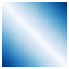
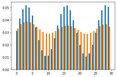
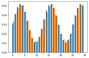
Figure 1: Effect of the regularization. Upper plots, from left to right: cost matrix used, transportation matrix for $\varepsilon=\eta-\varepsilon=0.1$ after $10^{5}$ iterations, and for $\varepsilon=\eta-\varepsilon=0.01$. Lower plots, from left to right: Target measure $\mu$ in blue, estimator in orange, $\varepsilon=\eta-\varepsilon=0.1$, then for $\varepsilon=\eta-\varepsilon=0.01$.

The regularization term $\eta$ should be greater than $\varepsilon$, and brings the estimated measure closer to the uniform measure. We choose to take $\eta=2\varepsilon$ to conserve a similar degree of regularization as in the case $\eta=0$, while guaranteeing that the exponentials in (14) do not overflow.

Sensibility to dimension.

We consider the relationship between the convergence rate and the dimensions $(I,J)$ of the problem. The theoretical results 5.1 and 5.2 depend on $(\min_{i}\mu_{i})+(\min_{j}\beta_{j})$, which scales with $1/\min(I,J)$ if $\mu$ and $\beta$ are uniform on their support. We generate $\mathcal{X}$ and $\mathcal{Y}$ as two samples of $I$ and $J$ independent Gaussian vectors, $\mu$ is the uniform measure on $\mathcal{X}$, and $C_{i,j}$ is the distance matrix between $X_{i}$ and $Y_{j}$. We compute the gradient norm of the objective function $F$ at the averaged iterates $\overline{a_{t}},$ $\overline{b_{t}}$.

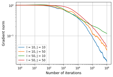
Figure 2: Convergence of the gradient norm for different dimensions.

The gradient norm here converges at rate $O(T^{-\delta})$, with $\delta\geq 1/2$ as would be predicted from the theorem 5.1, except in the case $I>J$ where $1/4\leq\delta<1/2$, which matches better with the bound in Theorem 5.2. An increase of the sample size $I$ for the input measure seems to decrease performance while an increase of the support size $J$ of the target increases performance. It means that a finer grid of points in $\mathcal{Y}$ will provide a faster convergence to the optimal estimator.

Choice of the learning rate.

As noted above, a choice of learning rate that is large compared to $\varepsilon$ can lead to a divergence of the dual variables. This is due to the exponential dependency of the gradients in $a$ and $b$. Experiments suggest the learning rate

$$\gamma_{t}=\min\left\{\frac{1}{\lambda t},\frac{c_{0}\varepsilon}{\sqrt{t}}\right\}.$$

The following graphs show the convergence to the target with different choices of $c_{0}$. Here $\varepsilon=0.001$, $\eta=0.002$, with the same problem is the same as in the experiments on the regularization term.

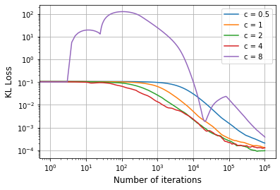
Figure 3: Comparison of the learning rates.

A regression on the curves shows that the empirical convergence rate is of order $O\left(T^{-\delta}\right)$ with $\delta>1$, which matches with theorem 5.1. We remark that the greater $c_{0}$ is, the better the algorithm converges, until it becomes unstable and does not converge anymore for $c_{0}>5$. This instability was observed consistently for a large range of values of $\varepsilon$ and $\eta$. The choice $c_{0}=2$ appears to be reasonable for both stability and convergence.

6 Conclusion

We consider the problem of minimizing a doubly regularized optimal transport cost over a set of finitely supported measures with fixed support. Using an entropic regularization on the target measure, we derive a stochastic gradient descent on the dual formulation with sublinear (even constant in the simplest case) complexity at each step of the optimization. The algorithm is thus highly paralellizable, and can be used to compute a regularized solution to the Wasserstein barycenter problem. We also provide convergence bounds for the estimator that this algorithm yields after $t$ steps, and demonstrate its performs on randomly generated data.

Aknowledgements.

This work was funded in part by the French government under management of Agence Nationale de la Recherche as part of the “Investissements d’avenir” program, reference ANR-19-P3IA-0001 (PRAIRIE 3IA Institute). We also acknowledge support from the European Research Council (grant SEQUOIA 724063).

Appendix A Proofs of technical results

Proof of proposition 2.1.

This proof follows the reasoning in Rigollet and Weed (2018). Let $\mu=\frac{1}{I}\sum_{i}\delta_{X_{i}}$ be the empirical measure of the sample $(X_{i})$. We first remark that the log-likelihood of $X_{i}$ defined by

$$\ell_{\nu}(X_{i}):=\log\int\kappa(X_{i},y)d\nu(y)$$

verifies

$$\ell_{\nu}(X_{i})=\log\mathbb{E}_{Y\sim\nu}\left[\kappa(X_{i},Y)\right].$$

With the Legendre transform of the relative entropy, we obtain

$$\ell_{\nu}(X_{i})=\sup_{\gamma_{i}}\mathbb{E}_{Y\sim\gamma_{i}}\left[\log\kappa(X_{i},Y)\right]-\text{KL}(\gamma_{i},\nu)$$

with the minimum being over every probability measures $\gamma_{i}$ on $\mathcal{Y}$. The MLE maximizes

$$\frac{1}{I}\sum_{i}\ell_{\nu}(X_{i})=\mathbb{E}_{X\sim\mu}\left[\ell_{\nu}(X)\right]$$

over $\nu\in\mathcal{M}$, it can be written as

$$\max_{\pi\in\Pi(\mu,\nu)}\mathbb{E}_{(X,Y)\sim\pi}\left[\log\kappa(X,Y)\right]-\mathbb{E}_{X\sim\mu}\left[KL(\pi(X,\cdot),\nu)\right],$$

with $\pi(X,\cdot)$ being the conditional probability of $\pi$, defined by $\pi(X_{i},\cdot):=\gamma_{i}$. We have

$$\mathbb{E}_{X\sim\mu}\left[KL(\pi(X,\cdot),\nu)\right]= \frac{1}{I}\sum_{i}\mathbb{E}_{Y\sim\nu}\left[\log\frac{d\pi(X_{i},\cdot)}{d\nu}(Y)\right],$$

$$= \frac{1}{I}\sum_{i}\mathbb{E}_{Y\sim\nu}\left[\log\frac{d\pi}{d\mu\otimes\nu}(X_{i},Y)\right]-\log I,$$

$$= KL(\pi,\mu\otimes\nu)-\log I.$$

Thus the MLE minimizes

$$\min_{\pi\in\Pi(\mu,\nu)}\mathbb{E}\left[c(X,Y)\right]+\varepsilon\text{KL}(\pi,\mu\otimes\nu),$$

which is the regularized optimal transport cost between $\mu$ and $\nu$. ∎

Proof of Proposition 3.3.

1. The function $H_{\beta,\mathcal{M}}^{*}$ is a Legendre transform, so it is convex, and thus $-F$ is convex as a sum of convex functions. Moreover $F$ is bounded from above:

   $$F(a,b)\leq C_{1}\mathbb{E}[a_{i}+b_{j}]-C_{2}\mathbb{E}\left[e^{\frac{a_{i}+b_{j}}{\varepsilon}}\right],$$

   $$\leq C_{3},$$

   where $C_{3}$ does not depend on $a$ or $b$. Thus the set of solutions is nonempty. F is invariant by the translation $(a,b)\mapsto(a_{1}+c,\dots,a_{I}+c,b_{1}-c,\dots,b_{J}-c)$, so each solution generates an affine set of solutions spanned by the vector $((1,\dots,1),(-1,\dots,-1))$. We can conclude using the strong convexity on the slice $\{\sum_{i}\mu_{i}a_{i}=\sum_{j}\beta_{j}b_{j}\}$, which implies that there exists only one solution on this slice.

2. The solution $(a^{*},b^{*})$ solves the following system

   $$\begin{cases}\nabla_{a}F(a^{*},b^{*})=0,\\ \nabla_{b}F(a^{*},b^{*})=0.\end{cases}$$

   With notations $A_{i}=e^{a^{*}_{i}/\varepsilon}$, $B_{j}=e^{b^{*}_{j}/\varepsilon}$, $\Gamma_{i,j}=e^{-C_{i,j}/\varepsilon}$, the two equations can be written as

   $$\begin{cases}\forall\ 1\leq i\leq I,&1-A_{i}\sum_{j}\beta_{j}B_{j}\Gamma_{i,j}=0,\\ \forall\ 1\leq j\leq J,&f_{j}-B_{j}\sum_{i}\mu_{i}A_{i}\Gamma_{i,j}=0.\end{cases}$$ (18)

   Thus

   $$\begin{cases}\forall\ 1\leq i\leq I,&A_{i}=\frac{1}{\sum_{j}\beta_{j}B_{j}\Gamma_{i,j}},\\ \forall\ 1\leq j\leq J,&B_{j}=\frac{f_{j}}{\sum_{i}\mu_{i}A_{i}\Gamma_{i,j}}.\end{cases}$$ (19)

   We also remark that by multiplying the second term of (18) by $\beta_{j}$ and summing over $j$ we get

   $$\sum_{i,j}\mu_{i}A_{i}\beta_{j}B_{j}\Gamma_{i,j}=1.$$ (20)

   By multiplying the equations in (19) we have for all $i,j$:

   $$A_{i}B_{j}\Gamma_{i,j}=\frac{f_{j}\Gamma_{i,j}}{\sum_{k,l}\mu_{k}A_{k}\Gamma_{k,j}\beta_{l}B_{l}\Gamma_{i,l}}$$

   thus using (20):

   $$f_{j}\min_{k,l}\frac{\Gamma_{i,j}\Gamma_{k,l}}{\Gamma_{k,j}\Gamma_{i,l}}\leq A_{i}B_{j}\Gamma_{i,j}\leq f_{j}\max_{k,l}\frac{\Gamma_{i,j}\Gamma_{k,l}}{\Gamma_{k,j}\Gamma_{i,l}}$$

   finally

   $$e^{-m-2R_{C}/\varepsilon}\leq A_{i}B_{j}\Gamma_{i,j}\leq e^{m+2R_{C}/\varepsilon}.$$

3. We now prove that $-F$ is strongly convex. We compute

   $$-\nabla_{a}^{2}F=\mathbb{E}\left[\frac{1}{\varepsilon}D_{i,j}E_{i,i}\right],$$

   $$-\nabla_{b}^{2}F=-\nabla_{b}\nu^{*}+\mathbb{E}\left[\frac{1}{\varepsilon}D_{i,j}E_{j,j}\right],$$

   $$-\nabla_{a}\nabla_{b}F=\mathbb{E}\left[\frac{1}{\varepsilon}D_{i,j}E_{i,j}\right].$$

   We remark that

   $$\nu^{*}=\text{softmax}(-b_{j}/\eta+\log\beta_{j}),$$

   so

   $$-\nabla_{b}\nu^{*}=\frac{1}{\eta}S$$

   with

   $$S:=(\nabla\text{softmax})(-b_{j}/\eta+\log\beta_{j}),$$

   $$S=(\nu_{i}(\delta_{i,j}-\nu_{j}))_{i,j}.$$

   We remark that $S\succcurlyeq 0$ since

   $$u^{T}Su =\sum_{i}\nu_{i}u_{i}^{2}-\left(\sum_{i}\nu_{i}u_{i}\right)^{2}$$

   $$=\mathbb{E}_{\nu}[U^{2}]-\left(\mathbb{E}_{\nu}[U]\right)^{2}\geq 0$$

   by Jensen, with $U=u_{j}$ with probability $\nu_{j}$. It implies $-\nabla_{b}\nu_{j}^{*}\succcurlyeq 0$. So

   $$-\nabla_{a,b}^{2}F\succcurlyeq\frac{1}{\varepsilon}M,$$

   with

   $$M:=\mathbb{E}\left[D_{i,j}\left(\begin{matrix}E_{i,i}&E_{i,j}\\ E_{j,i}&E_{j,j}\end{matrix}\right)\right].$$

   As we want to prove strong convexity on the slice $\sum_{i}\mu_{i}a_{i}=\sum_{j}\beta_{j}b_{j}$, we compute

   $$(a,b)^{T}M(a,b)=\mathbb{E}\left[D_{i,j}(a_{i}+b_{j})^{2}\right]\geq e^{-B/\varepsilon}\mathbb{E}\left[(a_{i}+b_{j})^{2}\right].$$

   We add that

   $$\mathbb{E}\left[(a_{i}+b_{j})^{2}\right]=\sum_{i}\mu_{i}a_{i}^{2}+\sum_{j}\beta_{j}b_{j}^{2}+2(\sum_{i}\mu_{i}a_{i})(\sum_{j}\beta_{j}b_{j})$$

   thus

   $$\mathbb{E}\left[(a_{i}+b_{j})^{2}\right]=\sum_{i}(\mu_{i}+\mu_{i}^{2})a_{i}^{2}+\sum_{j}(\beta_{j}+\beta_{j}^{2})b_{j}^{2}$$

   since we are on the slice. So $M\succcurlyeq\lambda\text{Id}$ and finally $-F$ is $\lambda-$strongly convex with

   $$\lambda=\frac{\min_{i,j}\{\mu_{i},\beta_{j}\}}{\varepsilon}e^{-B/\varepsilon}.$$

4. We compute the gradients of $F$:

   $$\frac{\partial F}{\partial a_{i}}(a,b) =\mu_{i}-\mu_{i}\sum_{j=1}^{J}\beta_{j}D_{i,j}(a,b),$$ (21)

   $$\frac{\partial F}{\partial b_{j}}(a,b) =\nu_{j}^{*}(-b/\eta)-\beta_{j}\sum_{i=1}^{I}\mu_{i}D_{i,j}(a,b),$$ (22)

   with $D_{i,j}(a,b)=e^{\frac{a_{i}+b_{j}-C_{i,j}}{\varepsilon}}$. If we take $i$ and $j$ to be independent random variables following the laws $(\mu_{i})$ and $(\beta_{j})$ respectively, we have the desired expression for the gradients.

∎

Proof of Lemma 1.

With the initial conditions, we guarantee that $0\leq G_{a}^{0}\leq 1$ and $0\leq G_{b}^{0}\leq f_{j}\leq e^{m}$. At each timestep $t$, we have

$$\|\nabla F_{i,j}^{t}\|^{2}\leq\max\{2e^{2m},2(D_{i,j}^{t})^{2}\},$$

with $i,j$ being two independent random variables following the laws $\mu$ and $\beta$ respectively. If $D_{i,j}^{t}\geq e^{m}$, then $G_{a}+G_{b}\leq 0$ and

$$D_{i,j}^{t+1}=D_{i,j}^{t}e^{\frac{G_{a}+G_{b}}{\varepsilon}}\leq D_{i,j}^{t}.$$

Moreover if $D_{i,j}^{t}\leq e^{m}$ then $\|\nabla F_{i,j}^{t}\|^{2}\leq 1+e^{2m}$ thus $\mathbb{E}\left[\max\{2e^{2m},(D_{i,j}^{t})^{2}\}\right]$ is a decreasing function of $t$. Thus we have the bound

$$\mathbb{E}\left[\|\nabla_{a}F_{i,j}(a^{t},b^{t})\|^{2}+\|\nabla_{b}F_{i,j}(a^{t},b^{t})\|^{2}\right]\leq 2e^{2m}.$$

∎

Proof of Lemma 2.

We first assume that $(a,b)$ and $(a^{*},b^{*})$ are on the slice $\{\sum_{i}\mu_{i}a_{i}=\sum_{j}\beta_{j}b_{j}\}$. By strong convexity of $-F$ on this slice we have

$$|b-b^{*}|^{2}\leq\frac{2(F(a^{*},b^{*})-F(a,b))}{\lambda}.$$ (23)

We remark that the function $g:b\mapsto KL(\nu(b^{*}),\nu(b))$ verifies

$$\partial_{i}g(b) =-\sum_{j}\nu_{j}(b^{*})\partial_{i}\log\nu_{j}(b),$$

$$=-\sum_{j}\nu_{j}(b^{*})\nu_{j}(b)^{-1}\partial_{i}\nu_{j}(b),$$

$$=\frac{1}{\eta}\sum_{j}\nu_{j}(b^{*})\nu_{j}(b)^{-1}\nu_{i}(\delta_{ij}-\nu_{j}(b)),$$

$$=\frac{\nu_{i}(b^{*})-\nu_{i}(b)}{\eta-\varepsilon},$$

thus

$$\partial_{i}\partial_{j}g(b) =-\frac{\partial_{j}\nu_{i}(b)}{\eta-\varepsilon},$$

$$=-\frac{\nu_{j}(b)(\delta_{ij}-\nu_{i}(b))}{\eta-\varepsilon},$$

so the Hessian matrix $\nabla^{2}g(b)$ of $g$ is a sum of a diagonal matrix with the negative values $-\nu_{j}(b)/(\eta-\varepsilon)$ and the one-rank matrix $(\nu_{j}(b)\nu_{i}(b)/(\eta-\varepsilon))_{i,j}$. Hence the eigenvalues of $\nabla^{2}g(b)$ are contained in $[-1/(\eta-\varepsilon),1/(\eta-\varepsilon)]$, thus Taylor’s inequality gives

$$g(b) \leq g(b^{*})+|b-b^{*}|\|\nabla g(b^{*})\|+\frac{|b-b^{*}|^{2}}{2(\eta-\varepsilon)},$$

$$\leq\frac{|b-b^{*}|^{2}}{2(\eta-\varepsilon)},$$

because $g(b^{*})=0$ and $\nabla g(b^{*})=0$. We complete the proof with (23). For the case where the vector $(a,b)$ or $(a^{*},b^{*})$ is not on the slice $\{\sum_{i}\mu_{i}a_{i}=\sum_{j}\beta_{j}b_{j}\}$, we note that adding a constant vector $c=(c_{1},\dots,c_{1})$ to $b$ does not change the value of $\nu(b)$, and that $F$ is invariant by translation in the direction $(-c,+c)$. With $c_{1}=\left(\sum_{i}\mu_{i}a_{i}-\sum_{j}\beta_{j}b_{j}\right)/2$, the vectors $(a^{\prime},b^{\prime})=(a+c,b-c)$ are on the slice and verify $\nu(b^{\prime})=\nu(b)$ and $F(a^{\prime},b^{\prime})=F(a,b)$. Hence the result for $(a^{\prime},b^{\prime})$ implies the result for $(a,b)$. ∎

References

• Agueh and Carlier (2011) Martial Agueh and Guillaume Carlier. Barycenters in the wasserstein space. SIAM Journal on Mathematical Analysis, 43(2):904–924, 2011.
• Alaux et al. (2019) Jean Alaux, Edouard Grave, Marco Cuturi, and Armand Joulin. Unsupervised hyper-alignment for multilingual word embeddings. 2019.
• Altschuler et al. (2017) Jason Altschuler, Jonathan Niles-Weed, and Philippe Rigollet. Near-linear time approximation algorithms for optimal transport via sinkhorn iteration. In Advances in Neural Information Processing Systems, pages 1964–1974, 2017.
• Alvarez-Melis et al. (2018) David Alvarez-Melis, Tommi Jaakkola, and Stefanie Jegelka. Structured optimal transport. In International Conference on Artificial Intelligence and Statistics, pages 1771–1780, 2018.
• Arbel et al. (2019) Michael Arbel, Anna Korba, Adil Salim, and Arthur Gretton. Maximum mean discrepancy gradient flow. In Advances in Neural Information Processing Systems, pages 6481–6491, 2019.
• Arjovsky et al. (2017) Martin Arjovsky, Soumith Chintala, and Léon Bottou. Wasserstein generative adversarial networks. In International Conference on Machine Learning, pages 214–223, 2017.
• Bassetti et al. (2006) Federico Bassetti, Antonella Bodini, and Eugenio Regazzini. On minimum kantorovich distance estimators. Statistics & probability letters, 76(12):1298–1302, 2006.
• Berthet and Kanade (2019) Quentin Berthet and Varun Kanade. Statistical windows in testing for the initial distribution of a reversible markov chain. pages 246–255, 2019.
• Boursier and Perchet (2019) Etienne Boursier and Vianney Perchet. Private learning and regularized optimal transport. arXiv preprint arXiv:1905.11148, 2019.
• Claici et al. (2018) Sebastian Claici, Edward Chien, and Justin Solomon. Stochastic wasserstein barycenters. In International Conference on Machine Learning, pages 999–1008, 2018.
• Clarkson et al. (2012) Kenneth L. Clarkson, Elad Hazan, and David P Woodruff. Sublinear optimization for machine learning. Journal of the ACM (JACM), 59(5):1–49, 2012.
• Cuturi (2013) Marco Cuturi. Sinkhorn distances: Lightspeed computation of optimal transport. In Advances in neural information processing systems, pages 2292–2300, 2013.
• Cuturi and Doucet (2014) Marco Cuturi and Arnaud Doucet. Fast computation of wasserstein barycenters. In International Conference on Machine Learning, pages 685–693, 2014.
• del Barrio et al. (2019) Eustasio del Barrio, Hristo Inouzhe, Jean-Michel Loubes, Carlos Matrán, and Agustín Mayo-Íscar. optimalflow: Optimal-transport approach to flow cytometry gating and population matching. arXiv preprint arXiv:1907.08006, 2019.
• Dvurechensky et al. (2018) Pavel Dvurechensky, Alexander Gasnikov, and Alexey Kroshnin. Computational optimal transport: Complexity by accelerated gradient descent is better than by sinkhorn’s algorithm. In International Conference on Machine Learning, pages 1367–1376, 2018.
• Feydy et al. (2017) Jean Feydy, Benjamin Charlier, François-Xavier Vialard, and Gabriel Peyré. Optimal transport for diffeomorphic registration. In International Conference on Medical Image Computing and Computer-Assisted Intervention, pages 291–299. Springer, 2017.
• Feydy et al. (2019) Jean Feydy, Thibault Séjourné, François-Xavier Vialard, Shun-ichi Amari, Alain Trouve, and Gabriel Peyré. Interpolating between optimal transport and mmd using sinkhorn divergences. In The 22nd International Conference on Artificial Intelligence and Statistics, pages 2681–2690, 2019.
• Flamary et al. (2018) Rémi Flamary, Marco Cuturi, Nicolas Courty, and Alain Rakotomamonjy. Wasserstein discriminant analysis. Machine Learning, 107(12):1923–1945, 2018.
• Genevay et al. (2016) Aude Genevay, Marco Cuturi, Gabriel Peyré, and Francis Bach. Stochastic optimization for large-scale optimal transport. In Advances in neural information processing systems, pages 3440–3448, 2016.
• Genevay et al. (2017) Aude Genevay, Gabriel Peyré, and Marco Cuturi. Learning generative models with sinkhorn divergences. arXiv preprint arXiv:1706.00292, 2017.
• Genevay et al. (2019) Aude Genevay, Lénaïc Chizat, Francis Bach, Marco Cuturi, and Gabriel Peyré. Sample complexity of sinkhorn divergences. In The 22nd International Conference on Artificial Intelligence and Statistics, pages 1574–1583, 2019.
• Gordaliza et al. (2019) Paula Gordaliza, Eustasio Del Barrio, Gamboa Fabrice, and Jean-Michel Loubes. Obtaining fairness using optimal transport theory. In International Conference on Machine Learning, pages 2357–2365, 2019.
• Grave et al. (2019) Edouard Grave, Armand Joulin, and Quentin Berthet. Unsupervised alignment of embeddings with wasserstein procrustes. In The 22nd International Conference on Artificial Intelligence and Statistics, pages 1880–1890, 2019.
• Gretton et al. (2012) Arthur Gretton, Karsten M Borgwardt, Malte J Rasch, Bernhard Schölkopf, and Alexander Smola. A kernel two-sample test. Journal of Machine Learning Research, 13(Mar):723–773, 2012.
• Kantorovich (2006) Leonid V Kantorovich. On the translocation of masses. Journal of Mathematical Sciences, 133(4):1381–1382, 2006.
• Kuhn (1955) Harold W Kuhn. The hungarian method for the assignment problem. Naval research logistics quarterly, 2(1-2):83–97, 1955.
• Lavenant et al. (2018) Hugo Lavenant, Sebastian Claici, Edward Chien, and Justin Solomon. Dynamical optimal transport on discrete surfaces. ACM Transactions on Graphics (TOG), 37(6):1–16, 2018.
• Luise et al. (2018) Giulia Luise, Alessandro Rudi, Massimiliano Pontil, and Carlo Ciliberto. Differential properties of sinkhorn approximation for learning with wasserstein distance. In Advances in Neural Information Processing Systems, pages 5859–5870, 2018.
• Luise et al. (2019) Giulia Luise, Saverio Salzo, Massimiliano Pontil, and Carlo Ciliberto. Sinkhorn barycenters with free support via frank-wolfe algorithm. In Advances in Neural Information Processing Systems, pages 9318–9329, 2019.
• Monge (1781) Gaspard Monge. Mémoire sur la théorie des déblais et des remblais. Histoire de l’Académie Royale des Sciences de Paris, 1781.
• Peyré et al. (2019) Gabriel Peyré, Marco Cuturi, et al. Computational optimal transport. Foundations and Trends® in Machine Learning, 11(5-6):355–607, 2019.
• Rigollet and Weed (2018) Philippe Rigollet and Jonathan Weed. Entropic optimal transport is maximum-likelihood deconvolution. Comptes Rendus Mathematique, 356(11-12):1228–1235, 2018.
• Schiebinger et al. (2019) Geoffrey Schiebinger, Jian Shu, Marcin Tabaka, Brian Cleary, Vidya Subramanian, Aryeh Solomon, Joshua Gould, Siyan Liu, Stacie Lin, Peter Berube, et al. Optimal-transport analysis of single-cell gene expression identifies developmental trajectories in reprogramming. Cell, 176(4):928–943, 2019.
• Shamir and Zhang (2012) Ohad Shamir and Tong Zhang. Stochastic gradient descent for non-smooth optimization: Convergence results and optimal averaging schemes. CoRR, abs/1212.1824, 2012.
• Sinkhorn (1964) Richard Sinkhorn. A relationship between arbitrary positive matrices and doubly stochastic matrices. The annals of mathematical statistics, 35(2):876–879, 1964.
• Solomon et al. (2015) Justin Solomon, Fernando De Goes, Gabriel Peyré, Marco Cuturi, Adrian Butscher, Andy Nguyen, Tao Du, and Leonidas Guibas. Convolutional wasserstein distances: Efficient optimal transportation on geometric domains. ACM Transactions on Graphics (TOG), 34(4):1–11, 2015.
• Staib et al. (2017) Matthew Staib, Sebastian Claici, Justin M Solomon, and Stefanie Jegelka. Parallel streaming wasserstein barycenters. In Advances in Neural Information Processing Systems, pages 2647–2658, 2017.
• Uppal et al. (2019) Ananya Uppal, Shashank Singh, and Barnabas Poczos. Nonparametric density estimation & convergence rates for gans under besov ipm losses. In Advances in Neural Information Processing Systems, pages 9086–9097, 2019.
• Villani (2008) Cédric Villani. Optimal transport: old and new, volume 338. Springer Science & Business Media, 2008.
• Weed et al. (2019) Jonathan Weed, Francis Bach, et al. Sharp asymptotic and finite-sample rates of convergence of empirical measures in wasserstein distance. Bernoulli, 25(4A):2620–2648, 2019.
• Zemel et al. (2019) Yoav Zemel, Victor M Panaretos, et al. Fréchet means and procrustes analysis in wasserstein space. Bernoulli, 25(2):932–976, 2019.