Computationally Tractable Riemannian Manifolds for Graph Embeddings

Abstract

Representing graphs as sets of node embeddings in certain curved Riemannian manifolds has recently gained momentum in machine learning due to their desirable geometric inductive biases, e.g., hierarchical structures benefit from hyperbolic geometry. However, going beyond embedding spaces of constant sectional curvature, while potentially more representationally powerful, proves to be challenging as one can easily lose the appeal of computationally tractable tools such as geodesic distances or Riemannian gradients. Here, we explore computationally efficient matrix manifolds, showcasing how to learn and optimize graph embeddings in these Riemannian spaces. Empirically, we demonstrate consistent improvements over Euclidean geometry while often outperforming hyperbolic and elliptical embeddings based on various metrics that capture different graph properties. Our results serve as new evidence for the benefits of non-Euclidean embeddings in machine learning pipelines.

1 Introduction

Before representation learning started gravitating around deep representations [7] in the last decade, a line of research that sparked interest in the early 2000s was based on the so called manifold hypothesis [6]. According to it, real-world data given in their raw format (e.g., pixels of images) lie on a low-dimensional manifold embedded in the input space. At that time, most manifold learning algorithms were based on locally linear approximations to points on the sought manifold (e.g., LLE [64], Isomap [70]) or on spectral methods (e.g., MDS [40], graph Laplacian eigenmaps [5]).

Back to recent years, two trends are apparent: (i) the use of graph-structured data and their direct processing by machine learning algorithms [14, 38, 23, 35], and (ii) the resurgence of the manifold hypothesis, but with a different flavor – being explicit about the assumed manifold and, perhaps, the inductive bias that it entails: hyperbolic spaces [55, 56, 29], spherical spaces [78], and Cartesian products of them [36, 71, 67]. While for the first two the choice can be a priori justified – e.g., complex networks are intimately related to hyperbolic geometry [44] – the last one, originally through the work of Gu et al. [36], is motivated through the presumed flexibility coming from its varying curvature. Our work takes that hypothesis further by exploring the representation properties of several irreducible spaces of non-constant sectional curvature. We use, in particular, Riemannian manifolds where points are represented as specific types of matrices and which are at the sweet spot between semantic richness and tractability.

With no additional qualifiers, graph embedding is a vaguely specified intermediary step used as part of systems solving a wide range of graph analytics problems [57, 75, 77, 83]. What they all have in common is the representation of certain parts of a graph as points in a continuous space. As a particular instance of that general task, here we embed nodes of graphs with structural information only (i.e., undirected and without node or edge labels), as the ones shown in Figure 1, in novel curved spaces, by leveraging the closed-form expressions of the corresponding Riemannian distance between embedding points; the resulting geodesic distances enter a differentiable objective function which “compares” them to the ground-truth metric given through the node-to-node graph distances. We focus on the representation capabilities of the considered matrix manifolds relative to the previously studied spaces by monitoring graph reconstruction metrics. We note that preserving graph structure is essential to downstream tasks such as link prediction [73, 82] and node classification [50, 75, 74].

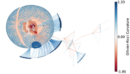
(a) “web-edu”

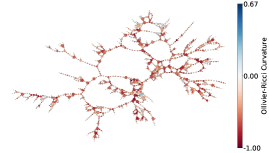
(b) “road-minnesota”

Figure 1: Two graphs used in our experiments: a web network from the .edu domain [32] and a road network in Minnesota [63]. The plots include the Ollivier-Ricci curvatures of edges and nodes. We refer the reader to Appendix C for details. More such visualizations are included in Appendix G.

Our main contributions include (i) the introduction of two families of matrix manifolds for graph embedding purposes: the non-positively curved spaces of symmetric positive definite (SPD) matrices, and the compact, non-negatively curved Grassmann manifolds; (ii) reviving Stochastic Neighbor Embedding (SNE) [39] in the context of Riemannian optimization as a way to unify, on the one hand, the loss functions based on the reconstruction likelihood of local graph neighborhoods and, on the other hand, the global, all-pairs stress functions used for global metric recovery; (iii) a generalization of the usual ranking-based metric to quantify reconstruction fidelity beyond immediate neighbors; (iv) a comprehensive experimental comparison of the introduced manifolds against the baselines in terms of their graph reconstruction capabilities, focusing on the impact of curvature.

Related Work.

Our work is inspired by the emerging field of geometric deep learning (GDL) [13] through its use of geometry. That being said, our motivation and approach are different. In GDL, deep networks transform data in a geometry-aware way, usually as part of larger discriminative or generative models: e.g., graph neural networks [14, 38], hyperbolic neural networks [30, 52, 37], hyperspherical neural networks [23, 80, 20], and others [3, 67]. We, on the other hand, embed graph nodes in a simpler, transductive setting, employing Riemannian optimization [10, 4] to directly obtain the corresponding embeddings. The broader aim to which we contribute is that of understanding the role played by the space curvature in graph representation learning. In this sense, works such as those of Sarkar [65] and Krioukov et al. [44], who formally describe the connections between certain types of graphs (i.e., trees and complex networks, respectively) and hyperbolic geometry, inspire us: ultimately, we seek similar results for new classes of graphs and embedding spaces. This work, mostly an empirical one, is a first step in that direction for two families of matrix manifolds. It is similar in spirit to Gu et al. [36] who empirically show that Cartesian products of model spaces can provide a good inductive bias in some cases. Finally, the manifolds themselves are not new in the machine learning literature: recent computer vision applications take into account the intrinsic geometry of SPD matrices [26, 41] and Grassmann subspaces [42, 81] when building discriminative models. It is the study of the implications of their curvature for graph representations that is novel.

2 Preliminaries & Background

Notation.

Let $G=(X,E,w)$ be an undirected graph, with $X$ the set of nodes, $E$ the set of edges, and $w:E\to\mathbb{R}_{+}$ the edge-weighting function. Let $m=\lvert X\rvert$. We denote by $d_{G}(x_{i},x_{j})$ the shortest path distance between nodes $x_{i},x_{j}\in X$, induced by $w$. The node embeddings are $Y=\{y_{i}\}_{i\in[m]}\subset\mathcal{M}$ and the geodesic distance function is $d_{\mathcal{M}}(y_{i},y_{j})$, with $\mathcal{M}$ – the embedding space – a Riemannian manifold. $\mathcal{N}(x_{i})$ denotes the set of neighbors of node $x_{i}$.

Riemannian Geometry.

A comprehensive account of the fundamental concepts from Riemannian geometry is included in Appendix A. Informally, an $n$-dimensional manifold $\mathcal{M}$ is a space that locally resembles $\mathbb{R}^{n}$. Each point $x\in\mathcal{M}$ has attached a tangent space $T_{x}\mathcal{M}$ – a vector space that can be thought of as a first-order local approximation of $\mathcal{M}$ around $x$. The Riemannian metric $\langle\cdot,\cdot\rangle_{x}$ is a collection of inner products on these tangent spaces that vary smoothly with $x$. It makes possible measuring geodesic distances, angles, and curvatures. The different notions of curvature quantify the ways in which a surface is locally curved around a point. The exponential map is a function $\exp_{x}:T_{x}\mathcal{M}\to\mathcal{M}$ that can be seen as “folding” or projecting the tangent space onto the manifold. Its inverse is called the logarithm map, $\log_{x}(\cdot)$.

Learning Framework.

The embeddings are learned in the framework used in recent prior work [55, 36] in which a loss function $\mathcal{L}$ depending on the embedding points solely via the Riemannian distances between them is minimized using stochastic Riemannian optimization [10, 4]. In this respect, the following general property is useful [46]: for any point $x$ on a Riemannian manifold $\mathcal{M}$ and any $y$ in a neighborhood of $x$, we have $\nabla_{x}^{R}\ d^{2}(x,y)=-2\log_{x}(y)$. Hence, as long as $\mathcal{L}$ is differentiable with respect to the (squared) distances, it will also be differentiable with respect to the embedding points. The specifics of $\mathcal{L}$ are deferred to Section 4.

Model Spaces & Cartesian Products.

The model spaces of Riemannian geometry are manifolds with constant sectional curvature $K$: (i) Euclidean space ($K=0$), (ii) hyperbolic space ($K<0$), and (iii) elliptical space ($K>0$). We summarize the Riemannian geometric tools of the last two in Appendix B. They are used as baselines in our experiments. We also recall that given a set of manifolds $\{\mathcal{M}_{i}\}_{i=1}^{k}$, the product manifold $\mathcal{M}=\bigtimes_{i=1}^{k}\mathcal{M}_{i}$ has non-constant sectional curvature and can be used for graph embedding purposes as long as each factor has efficient closed-form formulas for the quantities of interest [36].

Measuring Curvature around Embeddings.

Curvature properties are central to our work since they set apart the matrix manifolds discussed in Section 3. Recall that any manifold locally resembles Euclidean space. Hence, several ways of quantifying the actual space curvature between embeddings have been proposed; see Appendix C for an overview. One which we find more convenient for analysis and presentation purposes, because it yields bounded and easily interpretable values, is based on sums of angles in geodesic triangles formed by triples $x,y,z\in\mathcal{M}$,

$$k_{\theta}(x,y,z)=\theta_{x,y}+\theta_{x,z}+\theta_{y,z},\enskip\text{with}\ \theta_{x_{1},x_{2}}=\cos^{-1}\frac{\langle u_{1},u_{2}\rangle_{x_{3}}}{\left\lVert u_{1}\right\rVert_{x_{3}}\left\lVert u_{2}\right\rVert_{x_{3}}},\ u_{\{1,2\}}=\log_{x_{3}}(x_{\{1,2\}}).$$ (1)

It takes values in the intervals $[0,\pi]$ and $[\pi,3\pi]$, in hyperbolic and elliptical spaces, respectively. In practice, we look at empirical distributions of $\overline{k}_{\theta}=(k_{\theta}-\pi)/2\pi$, with values in $[-0.5,0]$ and $[0,1]$, respectively, obtained by sampling triples $(x,y,z)$ from an embedding set $\{y_{i}\}_{i=1}^{k}$.

3 Matrix Manifolds for Graph Embeddings

We propose two families of matrix manifolds that lend themselves to computationally tractable Riemannian optimization in our graph embedding framework. They cover negative and positive curvature ranges, respectively, resembling the relationship between hyperbolic and hyperspherical spaces. Their properties are summarized in Table 1. Details and proofs are included in Appendix D.

Table 1: Summary of Riemannian geometric tools for the SPD [8, 11, 43] and Grassmann [27, 81] manifolds. Notation: $A,B$ – manifold points; $P,Q$ – tangent space points; $P^{\prime}$ – ambient space point; $\exp(A)$  /  $\log(A)$ – matrix exponential / logarithm.

Property	SPD $\mathcal{S}^{\texttt{++}}(n)$	Grassmann $Gr(k,n)$
Dimension, $\dim(\mathcal{M})$	$n(n+1)/2$	$k(n-k)$
Tangent space, $T_{A}\,\mathcal{M}$	$\{A\in\mathbb{R}^{n\times n}:A=A^{\top}\}$	$\{P\in\mathbb{R}^{n\times k}:A^{\top}P=0\}$
Projection, $\pi_{A}(P^{\prime})$	$(P^{\prime}+P^{\prime\top})/2$	$(\operatorname{\mathop{\mathrm{Id}}}_{n}-AA^{\top})P^{\prime}$
Riem. metric, $\langle P,Q\rangle_{A}$	$\operatorname{\mathop{\mathrm{Tr}}}A^{-1}PA^{-1}Q$ $(2)$	$\operatorname{\mathop{\mathrm{Tr}}}P^{\top}Q$ $(3)$
Riem. gradient, $\nabla_{A}^{R}$	$A\,\pi_{A}(\nabla_{A}^{E})\,A$	$\pi_{A}(\nabla_{A}^{E})$
Geodesic, $\gamma_{A;P}(t)$	$A\exp(tA^{-1}P)$	$\begin{bmatrix}AV&U\end{bmatrix}\begin{bmatrix}\cos(t\Sigma)&\sin(t\Sigma)\end{bmatrix}V^{\top}$   with $P=U\Sigma V^{\top}$
Retraction, $R_{A}(P)$	$A+P+\frac{1}{2}PA^{-1}P$	$UV^{\top}$  with $A+P=U\Sigma V$
Log map, $\log_{A}(B)$	$A\log(A^{-1}B)$	$U\Sigma V^{\top}$  with $\begin{bmatrix}A^{\top}B\\ \big{(}\operatorname{\mathop{\mathrm{Id}}}_{n}-AA^{\top}\big{)}B\end{bmatrix}=\begin{bmatrix}V\cos(\Sigma)V^{\top}\\ U\sin(\Sigma)V^{\top}\end{bmatrix}$
Riem. dist., $d(A,B)$	$\left\lVert\log(A^{-1}B)\right\rVert_{F}$ $(4)$	$\sqrt{\sum_{i=1}^{k}\theta_{i}^{2}}$   with $A^{\top}B=U\operatorname{\mathop{\mathrm{diag}}}\big{(}\cos(\theta_{i})\big{)}V^{\top}$ $(5)$

3.1 Non-positive Curvature: SPD Manifold

The space of $n\times n$ real symmetric positive-definite matrices, $\mathcal{S}^{\texttt{++}}(n)\vcentcolon=\{A\in\mathcal{S}(n):\langle x,Ax\rangle>0\ \textrm{for all}\ x\neq 0\}$, is an $\frac{n(n+1)}{2}$-dimensional differentiable manifold – an embedded submanifold of $\mathcal{S}(n)$, the space of $n\times n$ symmetric matrices. Its tangent space can be identified with $\mathcal{S}(n)$.

Riemannian Structure.

The most common Riemannian metric endowed to $\mathcal{S}^{\texttt{++}}(n)$ is $\langle P,Q\rangle_{A}=\operatorname{\mathop{\mathrm{Tr}}}A^{-1}PA^{-1}Q$. Also called the canonical metric, it is motivated as being invariant to congruence transformations $\Gamma_{X}(A)=X^{\top}AX$, with $X$ an $n\times n$ invertible matrix [61]. The induced distance function is $d(A,B)=\sqrt{\sum_{i=1}^{n}\log^{2}\big{(}\lambda_{i}(A^{-1}B)\big{)}}$. It can be interpreted as measuring how well $A$ and $B$ can be simultaneously reduced to the identity matrix [18].

Properties.

The canonical SPD manifold has non-positive sectional curvature everywhere [8]. It is also a high-rank symmetric space [45]. The high-rank property tells us that there are at least planes of the tangent space on which the sectional curvature vanishes. Contrast this with the hyperbolic space which is also a symmetric space but where the only (intrinsic) flats are the geodesics. Moreover, only one degree of freedom can be factored out of the manifold $\mathcal{S}^{\texttt{++}}(n)$: it is isometric to $\mathcal{S}_{\ast}^{\texttt{++}}(n)\times\mathbb{R}$, with $\mathcal{S}_{\ast}^{\texttt{++}}(n)\vcentcolon=\{A\in\mathcal{S}^{\texttt{++}}(n):\det(A)=1\}$, an irreducible manifold  [24]. Hence, $\mathcal{S}^{\texttt{++}}$ achieves a mix of flat and negatively-curved areas that cannot be obtained via other Riemannian Cartesian products.

Alternative Metrics.

There are several other metrics that one can endow the SPD manifold with, yielding different geometric properties: the log-Euclidean metric [see, e.g., 2] induces a flat manifold, while the Bures-Wasserstein metric from quantum information theory [9] leads to a non-negatively curved manifold. The latter has been leveraged in [53] to embed graph nodes as elliptical distributions. Finally, a popular alternative to the (squared) canonical distance is the symmetric Stein divergence, $S(A,B)\vcentcolon=\log\det\big{(}\frac{A+B}{2}\big{)}-\frac{1}{2}\log\det(AB)$. It has been thoroughly studied in [68, 69] who prove that $\sqrt{S}$ is indeed a metric and that $S(A,B)$ shares many properties of the Riemannian distance function (1) such as congruence and inversion invariances as well as geodesic convexity in each argument. It is particularly appealing for backpropagation-based training due to its computationally efficient gradients (see below). Hence, we experiment with it too when matching graph metrics.

Computational Aspects.

We compute gradients via automatic differentiation [59]. Nonetheless, notice that if $A=UDU^{\top}$ is the eigendecomposition of a symmetric matrix with distinct eigenvalues and $\mathcal{L}$ is some loss function that depends on $A$ only via $D$, then $\frac{\partial\mathcal{L}}{\partial A}=U\frac{\partial\mathcal{L}}{\partial D}U^{\top}$ [31]. Computing geodesic distances requires the eigenvalues of $A^{-1}B$, though, which may not be symmetric. We overcome that by using the matrix $A^{-1/2}BA^{-1/2}$ instead which is SPD and has the same spectrum. Moreover, for the $2\times 2$ and $3\times 3$ cases, we use closed-form eigenvalue formulas to speed up our implementation. For the Stein divergence, the gradients can be computed in closed form as $\nabla_{A}S(A,B)=\frac{1}{2}(A+B)^{-1}-\frac{1}{2}A^{-1}$. We additionally note that many of the required matrix operations can be efficiently computed via Cholesky decompositions. See Appendix D for details.

3.2 Non-negative Curvature: Grassmann Manifold

The orthogonal group $O(n)$ is the set of $n\times n$ real orthogonal matrices. It is a special case of the compact Stiefel manifold $V(k,n)\vcentcolon=\{A\in\mathbb{R}^{n\times k}:A^{\top}A=\operatorname{\mathop{\mathrm{Id}}}_{k}\}$, i.e., the set of $n\times k$ “tall-skinny” matrices with orthonormal columns, for $k\leqslant n$. The Grassmannian is defined as the space of $k$-dimensional linear subspaces of $\mathbb{R}^{n}$. It is related to the Stiefel manifold in that every orthonormal $k$-frame in $\mathbb{R}^{n}$ spans a $k$-dimensional subspace of the $n$-dimensional Euclidean space. Similarly, every such subspace admits infinitely many orthonormal bases. This suggests the identification of the Grassmann manifold $Gr(k,n)$ with the quotient space $V(k,n)/O(k)$ (more about quotient manifolds in Appendix A). In other words, an $n\times k$ orthonormal matrix $A\in V(k,n)$ represents the equivalence class $[A]=\{AQ_{k}:Q_{k}\in O(k)\}\cong\operatorname{\mathop{\mathrm{span}}}(A)$, which is a single point on $Gr(k,n)$.

Riemannian Structure.

The canonical Riemannian metric of $Gr(k,n)$ is simply the Frobenius inner product (1). We refer to [27] for details on how it arises from its quotient geometry. The closed form formula for the Riemannian distance, shown in (1), depends on the set $\{\theta_{i}\}_{i=1}^{k}$ of so-called principal angles between two subspaces. They can be interpreted as the minimal angles between all possible bases of the two subspaces [81].

Properties.

The Grassmann manifold $Gr(k,n)$ is a compact, non-negatively curved manifold. As shown in [79], its sectional curvatures at $A\in Gr(k,n)$ satisfy $K_{A}(P,Q)=1$ (for $k=1,\ n>2$) and $0\leqslant K_{A}(P,Q)\leqslant 2$ (for $k>1,\ n>k$), for all $P,Q\in T_{A}\,Gr(k,n)$. Contrast this with the constant positive curvature of the sphere which can be made arbitrarily large by making $R\to 0$.

Computational Aspects.

Computing a geodesic distance requires the SVD decomposition of an $k\times k$, matrix which can be significantly smaller than the manifold dimension $k(n-k)$. For $k=2$, we use closed-form solutions for singular values. See Appendix D for details. Otherwise, we employ standard numerical algorithms. For the gradients, a result analogous to the one for eigenvalues from earlier (Section 3.1, [31]) makes automatic differentiation straight-forward.

4 Decoupling Learning and Evaluation

Recall that our goal is to preserve the graph structure given through its node-to-node shortest paths by minimizing a loss which encourages similar relative geodesic distances between node embeddings. Recent related work broadly uses local or global loss functions that focus on either close neighborhood information or all-pairs interactions, respectively. The methods that fall under the former emphasize correct placement of immediate neighbors, such as the one used in [55] for unweighted graphs:

$$\mathcal{L}_{\textrm{neigh}}(Y)=-\sum_{(i,j)\in E}\log\frac{\exp\big{(}-d_{\mathcal{M}}(y_{i},y_{j})\big{)}}{\sum_{k\in\mathcal{N}(i)}\exp\big{(}-d_{\mathcal{M}}(y_{i},y_{k})\big{)}}.$$ (6)

Those that fall under the latter, on the other hand, compare distances directly via loss functions inspired by generalized MDS [12], e.g.,

$$\mathcal{L}_{\textrm{stress}}(Y)=\sum_{i<j}\Big{(}d_{G}(x_{i},x_{j})-d_{\mathcal{M}}(y_{i},y_{j})\Big{)}^{2}\enskip\text{or}\enskip\mathcal{L}_{\textrm{distortion}}(Y)=\sum_{i<j}\left\lvert\frac{d_{\mathcal{M}}^{2}(y_{i},y_{j})}{d_{G}^{2}(x_{i},x_{j})}-1\right\rvert.$$ (7)

The two types of objectives yield embeddings with different properties. It is thus not surprising that each one of them has been coupled in prior work with a preferred metric quantifying reconstruction fidelity. The likelihood-based one is evaluated via the popular rank-based mean average precision (mAP), while the global, stress-like ones yield best scores when measured by the average distortion (AD) of the reference metric. See, e.g., [22] for their definitions.

To decouple learning and evaluation, as well as to get both fairer and more informative comparisons between embeddings spaces, we propose to optimize another loss function that allows explicitly moving in a continuous way on the representation scale ranging from “local neighborhoods patching,” as encouraged by (6), to the global topology matching, as measured by those from (7). In the same spirit, we propose a more fine-grained ranking metric that makes the trade-off clearer.

RSNE – Unifying Two Disparate Regimes.

We advocate training embeddings via a version of the celebrated Stochastic Neighbor Embedding (SNE) [39] adapted to the Riemannian setting. SNE works by attaching to each node a distribution defined over all other nodes and based on the distance to them. This is done for both the input graph distances, yielding the ground truth distribution, and for the embedding distances, yielding the model distribution. That is, with $j\neq i$, we have

$$p_{ij}\vcentcolon=p(x_{j}\mid x_{i})=\frac{\exp\big{(}-d_{G}^{2}(x_{i},x_{j})/T\big{)}}{Z_{p_{i}}}\enskip\text{and}\enskip q_{ij}\vcentcolon=q(y_{j}\mid y_{i})=\frac{\exp\big{(}-d_{\mathcal{M}}^{2}(y_{i},y_{j})\big{)}}{Z_{q_{i}}},$$ (8)

where $Z_{p_{i}}$ and $Z_{q_{i}}$ are the normalizing constants and $T$ is the input scale parameter. The original SNE formulation uses $\mathcal{M}=\mathbb{R}^{n}$. In this case, the probabilities are proportional to an isotropic Gaussian $\mathcal{N}(y_{j}\mid y_{i},T)$. As defined above, it is our (natural) generalization to Riemannian manifolds – RSNE. The embeddings are then learned by minimizing the sum of Kullback-Leibler (KL) divergences between $p_{i}\vcentcolon=p(\cdot\mid x_{i})$ and $q_{i}\vcentcolon=q(\cdot\mid y_{i})$: $\mathcal{L}_{\textrm{SNE}}(Y)\vcentcolon=\sum_{i=1}^{m}\operatorname{\mathop{\mathrm{D_{KL}}}}\big{[}p_{i}\parallel q_{i}\big{]}$. For $T\to 0$, it is easy to show that it recovers the local neighborhood regime from (6). For a large $T$, the SNE objective tends towards placing equal emphasis on the relative distances between all pairs of points, thus behaving similar to the MDS-like loss functions (7) [39, Section 6]. What we have gained is that the temperature parameter $T$ acts as a knob for controlling the optimization goal.

F1@k – Generalizing Ranking Fidelity.

We generalize the ranking fidelity metric in the spirit of mAP@k (e.g., [36]) for nodes that are $k$ hops away from a source node, with $k>1$. Recall that the motivation stems, for one, from the limitation of mean average precision to immediate neighbors, and, at the other side of the spectrum, from the sensitivity to absolute values of non-ranking metrics such as the average distortion. For an unweighted graph $G$, we denote by $L_{G}(u;k)$ the set of nodes that are exactly $k$ hops away from a source node $u$ (i.e., “on layer $k$”), and by $\mathcal{B}_{G}(v;u)$ the set of nodes that are closer to node $u$ than another node $v$. Then, for an embedding $f:G\to\mathcal{M}$, the precision and recall of a node $v$ in the shortest-path tree rooted at $u$, with $u\neq v$, are given by

$$P(v;u)\vcentcolon=\frac{\lvert\mathcal{B}_{G}(v;u)\cap\mathcal{B}_{\mathcal{M}}(f(v);f(u))\rvert}{\lvert\mathcal{B}_{\mathcal{M}}(f(v);f(u))\rvert}\enskip\text{and}\enskip R(v;u)\vcentcolon=\frac{\lvert\mathcal{B}_{G}(v;u)\cap\mathcal{B}_{\mathcal{M}}(f(v);f(u))\rvert}{\lvert\mathcal{B}_{G}(v;u)\rvert}.$$ (9)

They follow the conventional definitions. For instance, the numerator is the number of true positives: the nodes that appear before $v$ in the shortest-path tree rooted at $u$ and, at the same time, are embedded closer to $u$ than $v$ is. The definition of the F1 score of $(u,v)$, denoted by $F_{1}(v;u)$, follows naturally as the harmonic mean of precision and recall. Then, the F1@k metric is obtained by averaging the F1 scores of all nodes that are on layer $k\geqslant 1$, across all shortest-path trees. That is, $F_{1}(k)\vcentcolon=\frac{1}{c(k)}\sum_{u\in G}\ \sum_{v\in L_{G}(u;k)}F_{1}(v;u)$, with $c(k)=\sum_{u\in G}\lvert L_{G}(u;k)\rvert$. This draws a curve $\{(k,F_{1}(k))\}_{k\in[d(G)]}$, where $d(G)$ is the diameter of the graph.

5 Experiments

We restrict our experiments here to evaluating the graph reconstruction capabilities of the proposed matrix manifolds relative to the constant curvature baseline spaces. A thorough analysis via properties of nearest-neighbor graphs constructed from manifold random samples, inspired by [44], is included in Appendix E. It shows that the two matrix manifolds lead to distinctive network structures.

Training Details & Evaluation.

We start by computing all-pairs shortest-paths in all input graphs, performing max-scaling, and serializing them to disk. Then, for each manifold, we optimize a set of embeddings for several combinations of optimization settings and loss functions, including both the newly proposed Riemannian SNE, for several values of $T$, and the ones used in prior work (Section 4). Finally, because we are ultimately interested in the representation power of each embedding space, we report the best F1@1, area under the F1@k curve (AUC), and average distortion (AD), across those repetitions. This is in line with the experimental framework from prior works [55, 36] with the added benefit of treating the objective function as a nuisance. More details are included in Appendix F.

Synthetic Graphs.

We begin by showcasing the F1@k metric for several generated graphs in Figure 2. On the $10\times 10\times 10$ grid and the $1000$-nodes cycle all manifolds perform well. This is because every Riemannian manifold generalizes Euclidean space and Euclidean geometry suffices for grids and cycles (e.g., a cycle looks locally like a line). The more discriminative ones are the two other graphs – a full balanced tree (branching factor $r=4$ and depth $h=5$) and a cycle of 10 trees ($r=3$ and $h=4$). The best performing embeddings involve a hyperbolic component while the SPD ones rank between those and the non-negatively curved ones (which are indistinguishable). The results confirm our expectations: (more) negative curvature is useful when embedding trees. Finally, notice that the high-temperature RSNE regime used here encourages the recovery of the global structure (high AUC F1@k) more than the local neighborhoods (low individual F1@k values for small $k$).

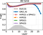
(a)

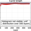
(b)

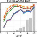
(c)

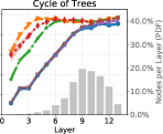
(d)

Figure 2: F1@k curves (left $y$-axis) and PMFs of node pairs per hop count (right $y$-axis) for several synthetic graphs. The objective was RSNE at high temperature $T$.

Non-positive Curvature.

We compare the Euclidean, hyperbolic, and SPD spaces on several real datasets in Table 2. For the SPD manifold, we experiment with both the canonical distance function and the (related) S-divergence as model metrics. When performing Riemannian optimization, we use the same canonical Riemannian tools (as per Table 1). More details about the graphs and an analysis of their geometric properties are attached in Appendix G. Two of the ones shown here are plotted in Figure 1. Extended results are included in Appendix H. First of all, we see that the (partial) negative curvature of the SPD and hyperbolic manifolds is beneficial: they outperform the flat Euclidean embeddings in almost all scenarios. This can be explained by the apparent scale-free nature of the input graphs [44]. Second, we see that especially when using the S-divergence, which we attribute to the better-behaved optimization task thanks to its geodesic convexity and stable gradients (see Section 3.1), the SPD embeddings achieve significant improvements on the average distortion metric and are competitive and sometimes better on the ranking metrics.

How Do the Embeddings Curve?

Since any manifold locally resembles Euclidean space, it is a priori unclear to what extent its theoretical curvature is leveraged by the embeddings. To shed light on that, we employ the analysis technique based on sum-of-angles in geodesic triangles from Section 2. We recognize in Figure 3 a remarkably consistent pattern: the better performing embeddings (as per Table 2) yield more negatively-curved triangles. Notice, for instance, the collapsed box plot corresponding to the “web-edu” hyperbolic embedding (a), i.e., almost all triangles sampled have sum-of-angles close to 0 . This is explained by its obvious tree-like structure (Figure 1a). Similarly, the SPD-Stein embedding of “facebook” outperforms the hyperbolic one in terms of F1@1 and that reflects in the slightly more stretched box plot (b). Moreover, the pattern applies to the best average-distortion embeddings, where the SPD-Stein embeddings are the only ones that make non-negligible use of negative curvature and, hence, perform better – the only exception is the “power” graph (c), for which indeed Table 2 confirms that the hyperbolic embeddings are slightly better.

Compact Embeddings.

We embed several graphs with traits associated with positive curvature in Grassmann manifolds and compare them to spherical embeddings. Table 3 shows that the former yields non-negligibly lower average distortion on the “cat-cortex” dissimilarity dataset and that the two are on-par on the “road-minnesota” graph (displayed in Figure 1b – notice its particular structure, characterized by cycles and low node degrees). More such results are included in Appendix H. As a general pattern, we find learning compact embeddings to be optimization-unfriendly.

Table 2: The results for “$\mathcal{S}^{\texttt{++}}$ vs. $\mathbb{H}$”. Best / second-best results are highlighted. The “Stein manifold” is SPD trained with the Stein divergence (see text). The F1@1 and AUC metrics are multiplied by 100.

$G$	$n$	$\mathcal{M}$	F1@1	AUC	AD
facebook	3	Euc	70.28	95.27	0.193
		Hyp	71.08	95.46	0.173
		SPD	71.09	95.26	0.170
		Stein	75.91	95.59	0.114
	6	Euc	79.60	96.41	0.090
		Hyp	81.83	96.53	0.089
		SPD	79.52	96.37	0.090
		Stein	83.95	96.74	0.061
web-edu	3	Euc	29.18	87.14	0.245
		Hyp	55.60	92.10	0.245
		SPD	29.02	88.54	0.246
		Stein	48.28	90.87	0.084
	6	Euc	49.31	91.19	0.143
		Hyp	66.23	95.78	0.143
		SPD	42.16	91.90	0.142
		Stein	62.81	96.51	0.043
bio-diseasome	3	Euc	83.78	91.21	0.145
		Hyp	86.21	95.72	0.137
		SPD	83.99	91.32	0.140
		Stein	86.70	94.54	0.105
	6	Euc	93.48	95.84	0.073
		Hyp	96.50	98.42	0.071
		SPD	93.83	95.93	0.072
		Stein	94.86	97.64	0.066
power	3	Euc	49.34	87.84	0.119
		Hyp	60.18	91.28	0.068
		SPD	52.48	90.17	0.121
		Stein	54.06	90.16	0.076
	6	Euc	63.62	92.09	0.061
		Hyp	75.02	94.34	0.060
		SPD	67.69	91.76	0.062
		Stein	70.70	93.32	0.049

Table 3: The results for “$Gr$ vs. $\mathbb{S}$”. The dataset “cat-cortex” [66] is a dissimilarity matrix, lacking graph connectivity information, so F1@k cannot be computed.

$G$	$n$	$\mathcal{M}$	F1@1	AUC	AD
road-minnesota	2	Sphere	82.19	94.02	0.085
		$Gr(1,3)$	78.91	94.02	0.085
	3	Sphere	89.55	95.89	0.059
		$Gr(1,4)$	90.02	95.88	0.058
	4	Sphere	93.65	96.66	0.049
		$Gr(1,5)$	93.89	96.67	0.049
		$Gr(2,4)$	94.01	96.66	0.049
cat-cortex	2	Sphere	-	-	0.255
		$Gr(1,3)$	-	-	0.234
	3	Sphere	-	-	0.195
		$Gr(1,4)$	-	-	0.168
	4	Sphere	-	-	0.156
		$Gr(1,5)$	-	-	0.139
		$Gr(2,4)$	-	-	0.129

Figure 3: Distributions of (normalized) sum-of-angles in geodesic triangles formed by the learned embeddings that yield the best F1@1 metrics (up) and the best average distortion metrics (down), for all datasets from Table 2, for $n=3$. 10000 triples are sampled.

6 Conclusion & Future Work

We proposed to use the SPD and Grassmann manifolds for learning representations of graphs and showed that they are competitive against previously considered constant-curvature spaces on the graph reconstruction task, consistently and significantly outperforming them in some cases. Our results suggest that their geometry can accommodate certain graphs with better precision and less distortion than other embedding spaces. We thoroughly described their properties, emphasizing those that set them apart, and worked out the practically challenging aspects. Moreover, we advocate the Riemannian SNE objective for learning embeddings as a way to unify two different families of loss functions used in recent related works. It allows practitioners to explicitly tune the desired optimization goal by adjusting the temperature parameter. Finally, we defined the F1@k metric as a more general way of quantifying ranking fidelity.

Our work is related to (and further motivates) some fundamental research questions. How does the curvature of a Riemannian manifold influence the types of metrics that it can represent? Can we design a theoretical framework that connects them to discrete metric spaces represented by graphs? How would a faithful embedding influence downstream tasks, such as node classification or link prediction? These are some of the questions we are excited about and plan to pursue in future work.

Broader Impact

Our research deals with a deeply technical question: how can we leverage geometry to better represent graphs? It is also part of a nascent area of machine learning that tries to improve existing methods by bringing forward geometry tools and theories which have been known in mathematics for a (relatively) long time. That being said, should it later materialize into practically useful applications, its impact can be significant. That is due to the ubiquity of graphs as models of data and the possibility for our research to improve graph-based models. To give several examples, our research can have a broader impact in network analysis (in particular, social networks), working with biological data (e.g., proteins, molecules), or learning from knowledge graphs. The impact of our work can be beneficial, for instance, when having more faithful graph models can lead to improved recommender systems or drug discovery. However, we emphasize that current models might suffer from various other modes of failure and, thus, are not capable of replacing human expertise and intervention.

Appendix A Overview of Differential & Riemannian Geometry

In this section, we introduce the foundational concepts from differential geometry, a discipline that has arisen from the study of differentiable functions on curves and surfaces, thus generalizing calculus. Then, we go a step further, into the more specific Riemannian geometry which enables the abstract definitions of lengths, angles, and curvatures. We base this section on [16, 1] and point the reader to them for a more thorough treatment of the subject.

Differentiable Manifolds.

Informally, an $n$-dimensional manifold is a set $\mathcal{M}$ which locally resembles $n$-dimensional Euclidean space. To be formal, one first introduces the notions of charts and atlases. A bijection $\varphi$ from a subset $\mathcal{U}\in\mathcal{M}$ onto an open subset of $\mathbb{R}^{n}$ is called an $n$-dimensional chart of the set $\mathcal{M}$, denoted by $(\mathcal{U},\varphi)$. It enables the study of points $x\in\mathcal{M}$ via their coordinates $\varphi(x)\in\mathbb{R}^{n}$. A differentiable atlas $\mathcal{A}$ of $\mathcal{M}$ is a collection of charts $(\mathcal{U}_{\alpha},\varphi_{\alpha})$ of the set $\mathcal{M}$ such that

1. $\bigcup_{\alpha}\mathcal{U}_{\alpha}=\mathcal{M}$

2. For any pair $\alpha,\beta$ with $\mathcal{U}_{\alpha}\cap\mathcal{U}_{\beta}\neq\emptyset$, the sets $\varphi_{\alpha}(\mathcal{U}_{\alpha}\cap\mathcal{U}_{\beta})$ and $\varphi_{\beta}(\mathcal{U}_{\alpha}\cap\mathcal{U}_{\beta})$ are open sets in $\mathbb{R}^{n}$ and the change of coordinates $\varphi_{\beta}\circ\varphi_{\alpha}^{-1}$ is smooth.

Two atlases $\mathcal{A}_{1}$ and $\mathcal{A}_{2}$ are equivalent if they generate the same maximal atlas. The maximal atlas $\mathcal{A}^{+}$ is the set of all charts $(\mathcal{U},\varphi)$ such that $\mathcal{A}\cup\{(\mathcal{U},\varphi)\}$ is also an atlas. It is also called a differentiable structure on $\mathcal{M}$. With that, an $n$-dimensional differentiable manifold is a couple $(\mathcal{M},\mathcal{A}^{+})$, with $\mathcal{M}$ a set and $\mathcal{A}^{+}$ a maximal atlas of $\mathcal{M}$ into $\mathbb{R}^{n}$. In more formal treatments, $\mathcal{A}^{+}$ is also constrained to induce a well-behaved topology on $\mathcal{M}$.

Embedded Submanifolds and Quotient Manifolds.

How is a differentiable structure for a set of interest usually constructed? From the definition above it is clear that it is something one endows the set with. That being said, in most useful cases it is not explicitly chosen or constructed. Instead, a rather recursive approach is taken: manifolds are obtained by considering either subsets or quotients (see last subsection paragraph) of other manifolds, thus inheriting a “natural” differentiable structure. Where does this recursion end? It mainly ends when one reaches a vector space, which is trivially a manifold via the global chart $\varphi:\mathbb{R}^{n\times k}\to\mathbb{R}^{nk}$, with $X\mapsto\mathrm{vec}(X)$. That is the case for the matrix manifolds considered in Section 3 too.

What makes the aforementioned construction approach (almost) assumption-free is the following essential property: if $\mathcal{M}$ is a manifold and $\mathcal{N}$ is a subset of the set $\mathcal{M}$ (respectively, a quotient $\mathcal{M}/{\sim}$), then there is at most one differentiable structure that agrees with the subset topology (respectively, with the quotient projection). The resulting manifolds are called embedded submanifolds and quotient manifolds, respectively. Sufficient conditions for their existence (hence, uniqueness) are known too and do apply for our manifolds. For instance, the submersion theorem says that for a smooth function $F:\mathcal{M}_{1}\to\mathcal{M}_{2}$ with $\dim(\mathcal{M}_{1})=d_{1}>d_{2}=\dim(\mathcal{M}_{2})$ and a point $y\in\mathcal{M}_{2}$ such that $F$ has full rank for all $x\in F^{-1}(y)$, its preimage $F^{-1}(y)$ is a closed embedded submanifold of $\mathcal{M}_{1}$ and $\dim(F^{-1}(y))=d_{1}-d_{2}$.

The quotient of a set $\mathcal{M}$ by an equivalence relation $\sim$ is defined as $\mathcal{M}/{\sim}\vcentcolon=\big{\{}[x]:x\in\mathcal{M}\big{\}}$, with $[x]\vcentcolon=\{y\in\mathcal{M}:y\sim x\}$ – the equivalence class of $x$. The function $\pi:\mathcal{M}\to\mathcal{M}/{\sim}$, given by $x\mapsto[x]$, is the canonical projection. The simplest example of a quotient manifold is the real projective space, $\mathbf{RP}(n-1)$. It is the set of lines through the origin in $\mathbb{R}^{n}$. With the notation $\mathbb{R}_{\ast}^{n}=\mathbb{R}^{n}\setminus\{0\}$, the real projective space can be identified with the quotient $\mathbb{R}_{\ast}^{n}/{\sim}$ given by the equivalence relation $x\sim y\iff\exists t\in\mathbb{R}_{\ast}:y=tx$.

Tangent Spaces.

To do even basic calculus on a manifold, one has to properly define the derivatives of manifold curves, $\gamma:\mathbb{R}\to\mathcal{M}$, as well as the directional derivatives of smooth real-valued functions defined on the manifold, $f:\mathcal{M}\to\mathbb{R}$. The usual definitions,

$$\gamma^{\prime}(t)\vcentcolon=\lim_{\tau\to 0}\frac{\gamma(t+\tau)-\gamma(t)}{\tau}\enskip\text{and}\enskip\operatorname{\textrm{D}}f(x)[\eta]\vcentcolon=\lim_{t\to 0}\frac{f(x+t\eta)-f(x)}{t},$$ (10)

are invalid as such because addition does not make sense on general manifolds. However, notice that $f\circ\gamma:t\mapsto f(\gamma(t))$ is differentiable in the usual sense. With that in mind, let $\mathfrak{T}_{x}(\mathcal{M})$ denote the set of smooth real-valued functions defined on a neighborhood of $x$. Then, the mapping $\dot{\gamma}(0)$ from $\mathfrak{T}_{x}(\mathcal{M})$ to $\mathbb{R}$ defined by

$$\dot{\gamma}(0)f\vcentcolon=\left.\frac{\mathrm{d}f(\gamma(t))}{\mathrm{d}t}\right|_{t=0}$$ (11)

is called the tangent vector to the curve $\gamma$ at $t=0$. The equivalence class

$$[\dot{\gamma}(0)]\vcentcolon=\{\gamma_{1}:\mathbb{R}\to\mathcal{M}:\dot{\gamma}_{1}(0)f=\dot{\gamma}(0)f,\ \forall f\in\mathfrak{T}_{x}\}$$ (12)

is a tangent vector at $x\in\mathcal{M}$. The set of such equivalence classes forms the tangent space $T_{x}\mathcal{M}$. It is immediate from the linearity of the differentiation operator from (11) that $T_{x}\mathcal{M}$ inherits a linear structure, thus forming a vector space.

The abstract definition from above recovers the classical definition of directional derivative from (10) in the following sense: if $\mathcal{M}$ is an embedded submanifold of a vector space $\mathcal{E}$ and $\overline{f}$ is the extension of $f$ in a neighborhood of $\gamma(0)\in\mathcal{E}$, then

$$\dot{\gamma}(0)f=\operatorname{\textrm{D}}\overline{f}(\gamma(0))[\gamma^{\prime}(0)],$$ (13)

so there is a natural identification of the mapping $\dot{\gamma}(0)$ with the vector $\gamma^{\prime}(0)$.

For quotient manifolds $\mathcal{M}/{\sim}$, the tangent space splits into two complementary linear subspaces called the vertical space $\mathcal{V}_{x}$ and the horizontal space $\mathcal{H}_{x}$. Intuitively, the vectors in the former point in tangent directions which, if we were to “follow” for an infinitesimal step, we would get another element of $[x]$. Thus, only the horizontal tangent vectors make us “move” on the quotient manifold.

Riemannian Metrics.

They are inner products $\langle\cdot,\cdot\rangle_{x}$, sometimes denoted by $g_{x}(\cdot,\cdot)$, attached to each tangent space $T_{x}\mathcal{M}$. They give a notion of length via $\left\lVert\xi_{x}\right\rVert_{x}\vcentcolon=\sqrt{\langle\xi_{x},\xi_{x}\rangle_{x}}$, for all $\xi_{x}\in T_{x}\mathcal{M}$. A Riemannian metric is an additional structure added to a differentiable manifold $(\mathcal{M},\mathcal{A}^{+})$, yielding the Riemannian manifold $(\mathcal{M},\mathcal{A}^{+},g_{x})$. However, as it was the case for the differentiable structure, for Riemannian submanifolds and Riemannian quotient manifolds it is inherited from the “parent” manifold in a natural way – see [1] for several examples.

The Riemannian metric enables measuring the length of a curve $\gamma:[a,b]\to\mathcal{M}$,

$$L(\gamma)=\int_{a}^{b}\sqrt{\langle\dot{\gamma}(t),\dot{\gamma}(t)\rangle_{\gamma(t)}}\mathrm{d}t,$$ (14)

which, in turn, yields the Riemannian distance function,

$$d_{\mathcal{M}}:\mathcal{M}\times\mathcal{M}\to\mathbb{R},\enskip d_{\mathcal{M}}(x,y)=\inf_{\gamma}L(\gamma),$$ (15)

that is, the shortest path between two points on the manifold. The infimum is taken over all curves $\gamma:[a,b]\to\mathcal{M}$ with $\gamma(a)=x$ and $\gamma(b)=y$. Note that in general it is only defined locally because $\mathcal{M}$ might have several connected components or it might not be geodesically complete (see next paragraphs). Deriving a closed-form expression of it is paramount for graph embedding purposes.

The Riemannian gradient of a smooth function $f:\mathcal{M}\to\mathbb{R}$ at $x$, denoted by $\nabla^{R}f(x)$ is defined as the unique element of $T_{x}\mathcal{M}$ that satisfies

$$\langle\nabla^{R}f(x),\xi\rangle_{x}=\operatorname{\textrm{D}}f(x)[\xi],\enskip\forall\xi\in T_{x}\mathcal{M}.$$ (16)

Retractions.

Up until this point, we have not introduced the concept of “moving in the direction of a tangent vector”, although we have appealed to this intuition. This is formally achieved via retractions. At a point $x\in\mathcal{M}$, the retraction $R_{x}$ is a map from $T_{x}\mathcal{M}$ to $\mathcal{M}$ satisfying local rigidity conditions: $R_{x}(0)=x$ and $\operatorname{\textrm{D}}R_{x}(0)=\operatorname{\mathop{\mathrm{Id}}}_{n}$. For embedded submanifolds, the two-step approach consisting of (i) taking a step along $\xi$ in the ambient space, and (ii) projecting back onto the manifold, defines a valid retraction. In quotient manifolds, the retractions of the base space that move an entire equivalence class to another equivalence class induce retractions on the quotient space.

Riemannian Connections.

Let us first briefly introduce and motivate the need for an additional structure attached to differentiable manifolds, called affine connections. They are functions

$$\nabla:\mathfrak{X}\times\mathfrak{X}\to\mathfrak{X},\enskip(\xi,\zeta)\to\nabla_{\xi}\zeta$$ (17)

where $\mathfrak{X}$ is the set of vector fields on $\mathcal{M}$, i.e., functions assigning to each point $x\in\mathcal{M}$ a tangent vector $\xi_{x}\in T_{x}\mathcal{M}$. They satisfy several properties that represent the generalization of the directional derivative of a vector field in Euclidean space. Affine connections are needed, for instance, to generalize second-order optimization algorithms, such as Newton’s method, to functions defined on manifolds.

The Riemannian connection, also known as the Levi-Civita connection, is the unique affine connection that, besides the properties referred to above, satisfies two others, one of which depends on the Riemannian metric – see [16] for details. It is the affine connection implicitly assumed when working with Riemannian manifolds.

Geodesics, Exponential Map, Logarithm Map, Parallel Transport.

They are all concepts from Riemannian geometry, defined in terms of the Riemannian connection. A geodesic is a curve with zero acceleration,

$$\nabla_{\dot{\gamma}(t)}\dot{\gamma}(t)=0.$$ (18)

Geodesics are the generalization of straight lines from Euclidean space. They are locally distance-minimizing and parameterized by arc-length. Thus, for every $\xi\in T_{x}\mathcal{M}$, there exists a unique geodesic $\gamma(t;x,\xi)$ such that $\gamma(0)=x$ and $\dot{\gamma}(0)=\xi$.

The exponential map is the function

$$\exp_{x}:\widehat{U}\subseteq T_{x}\mathcal{M}\to\mathcal{M},\enskip\xi\mapsto\exp_{x}(\xi)\vcentcolon=\gamma(1;x,\xi),$$ (19)

where $\widehat{U}$ is a neighborhood of $0$. The manifold is said to be geodesically complete if the exponential map is defined on the entire tangent space, i.e., $\widehat{U}=T_{x}\mathcal{M}$. It can be shown that $\exp_{x}(\cdot)$ is a retraction and satisfies the following useful property

$$d_{\mathcal{M}}\big{(}x,\ \exp_{x}(\xi)\big{)}=\left\lVert\xi\right\rVert_{x},\enskip\text{for all}\ \xi\in\widehat{U}.$$ (20)

The exponential map defines a diffeomorphism between a neighborhood of $0\in T_{x}\mathcal{M}$ onto a neighborhood of $x\in\mathcal{M}$. If we follow a geodesic $\gamma(t;x,\xi)$ from $t=0$ to infinity, it can happen that it is minimizing only up to $t_{0}<\infty$. If that is the case, the point $y=\gamma(t_{0};x,\xi)$ is called a cut point. The set of all such points, gathered across all geodesics starting at $x$, is called the cut locus of $\mathcal{M}$ at $x$, $\mathcal{C}(x)\subset\mathcal{M}$. It can be proven that the cut locus has finite measure [60]. The maximal domain where the exponential map is a diffeomorphism is given by its preimage on $\mathcal{M}\setminus\mathcal{C}(x)$. Hence, the inverse is called the logarithm map,

$$\log_{x}:\mathcal{M}\setminus\mathcal{C}(x)\to T_{x}\mathcal{M}.$$ (21)

The parallel transport of a vector $\xi_{x}\in T_{x}\mathcal{M}$ along a curve $\gamma:I\to\mathcal{M}$ is the unique vector field $\xi$ that points along the curve to tangent vectors, satisfying

$$\nabla_{\dot{\gamma}(t)}\xi\big{(}\gamma(t)\big{)}=0\enskip\text{and}\enskip\xi(x)=\xi_{x}.$$ (22)

Curvature.

The Riemann curvature tensor is a tensor field that assigns a tensor to each point of a Riemannian manifold. Each such tensor measures the extent to which the manifold is not locally isometric to Euclidean space. It is defined in terms of the Levi-Civita connection. For each pair of tangent vectors $u,v\in T_{x}\mathcal{M}$, $\operatorname{\mathrm{R}}_{x}(u,v)$ is a linear transformation on the tangent space. The vector $w^{\prime}=\operatorname{\mathrm{R}}_{x}(u,v)\,w$ quantifies the failure of parallel transport to bring $w$ back to its original position when following a quadrilateral determined by $-tu,-tv,tu,tv$, with $t\to 0$. This failure is caused by curvature and it is also known as the infinitesimal non-holonomy of the manifold.

The sectional curvature is defined for a fixed point $x\in\mathcal{M}$ and two tangent vectors $u,v\in T_{x}\mathcal{M}$ as

$$K_{x}(u,v)=\frac{\langle\operatorname{\mathrm{R}}_{x}(u,v)v,u\rangle_{x}}{\langle u,u\rangle_{x}\langle v,v\rangle_{x}-\langle u,v\rangle_{x}^{2}}.$$ (23)

It measures how far apart two geodesics emanating from $x$ diverge. If it is positive, the two geodesics will eventually converge. It is the most common curvature characterization that we use to compare, from a theoretical perspective, the manifolds discussed in this work.

The Ricci tensor $\operatorname{\mathrm{Ric}}(w,v)$ is defined as the trace of the linear map $T_{x}\mathcal{M}\to T_{x}\mathcal{M}$ given by $u\mapsto\operatorname{\mathrm{R}}(u,v)w$. It is fully determined by specifying the scalars $\operatorname{\mathrm{Ric}}(u,u)$ for all unit vectors $u\in T_{x}\mathcal{M}$, which is known simply as the Ricci curvature. It is equal to the average sectional curvature across all planes containing $u$ times $(n-1)$. Intuitively, it measures how the volume of a geodesic cone in direction $u$ compares to that of an Euclidean cone.

Finally, the scalar curvature (or Ricci scalar) is the most coarse-grained notion of curvature at a point on a Riemannian manifold. It is the trace of the Ricci tensor, or, equivalently, $n(n-1)$ times the average of all sectional curvatures. Note that a space of non-constant sectional curvature can have constant Ricci scalar. This is true, in particular, for homogeneous spaces (e.g., all manifolds studied in this work; see Appendix D).

Appendix B Differential Geometry Tools for Hyperbolic and Elliptical Spaces

Table 4: Summary of Riemannian geometric tools for hyperbolic and spherical spaces. Notation: $x,y\in\mathcal{M}$; $u,v\in T_{x}\mathcal{M}$; $\langle x,y\rangle_{L}$ – Lorentz product.

Property	Expr.	Hyperbolic $\mathbb{H}(n)$	Elliptical $\mathbb{S}(n)$
Representation	$\mathbb{H}(n)$ / $\mathbb{S}(n)$	$\{x\in\mathbb{R}^{n+1}:\langle x,x\rangle_{L}=-1,x_{0}>0\}$	$\{x\in\mathbb{R}^{n+1}:\left\lVert x\right\rVert_{2}=1\}$
Tangent space	$T_{x}\mathcal{M}$	$\{u\in\mathbb{R}^{n+1}:\langle u,x\rangle_{L}=0\}$	$\{u\in\mathbb{R}^{n+1}:x^{\top}u=0\}$
Projection	$\pi_{x}(u)$	$u+\langle u,x\rangle_{L}x$	$\big{(}\operatorname{\mathop{\mathrm{Id}}}_{n+1}-xx^{\top}\big{)}u$
Riem. metric	$\langle u,v\rangle_{x}$	$\langle u,v\rangle_{L}$	$\langle u,v\rangle$
Riem. gradient	$\nabla_{A}^{R}$	$\operatorname{\mathop{\mathrm{diag}}}(-1,1,\ldots,1)\pi_{x}(\nabla_{x}^{E})$	$\pi_{x}(\nabla_{x}^{E})$
Geodesics	$\gamma_{x;y}(t)$	$x\cosh(t)+y\sinh(t)$	$x\cos(t)+y\cos(t)$
Retraction	$R_{x}(u)$	Not used	Not used
Log map	$\log_{x}(y)$	$\frac{\cosh^{-1}(\alpha)}{\sqrt{\alpha^{2}-1}}(y-\alpha x)$    with $\alpha=-\langle x,y\rangle_{L}$	$\log_{x}(y)=\frac{\cos^{-1}(\langle x,y\rangle)}{\lVert u^{\prime}\rVert_{x}}u^{\prime}$    with $u^{\prime}=\pi_{x}(y-x)$
Riem. distance	$d(x,y)$	$\cosh^{-1}(-\langle x,y\rangle_{L})$	$\cos^{-1}(\langle x,y\rangle)$
Parallel transport	$\mathcal{T}_{x,y}(u)$	$u+\frac{\langle y-\alpha x,u\rangle_{L}}{\alpha+1}(x+y)$    with $\alpha=-\langle x,y\rangle_{L}$	$\pi_{b}(u)$
Characterizations		Constant negative curvature Isotropic	Constant positive curvature Isotropic

We include in Table 4 the differential geometry tools for the hyperbolic and elliptical spaces. We use the hyperboloid model for the former and the hyperspherical model for the latter, depicted in Figure 4. Some prior work prefers working with the Poincaré ball model and/or the stereographic projection. They have both advantages and disadvantages.

For instance, our choice yields simple formulas for certain quantities of interest, such as exponential and logarithm maps. They are also more numerically stable. In fact, it is claimed in [56] that numerical stability together with its impact on optimization are the only explanations for the Lorentz model outperforming the prior experiments in the (theoretically equivalent) Poincaré ball [55].

On the other hand, the just mentioned alternative models have the strong advantage that the corresponding metric tensors are conformal. This means that they are proportional to the Riemannian metric of Euclidean space,

$$g_{\mathbb{H}}=\bigg{(}\frac{2}{1-\lVert x\rVert_{2}^{2}}\bigg{)}^{2}g^{E}\enskip\text{and}\enskip g_{\mathbb{S}}=\bigg{(}\frac{2}{1+\lVert x\rVert_{2}^{2}}\bigg{)}^{2}g^{E}.$$ (24)

Notice the syntactic similarity between them. Furthermore, the effect of the denominators in the conformal factors reinforce the intuition we have about the two spaces: distances around far away points are increasingly larger in the hyperbolic space and increasingly smaller in the elliptical space.

Let us point out that both hyperbolic and elliptical spaces are isotropic. Informally, isotropy means “uniformity in all directions.” Note that this is a stronger property than the homogeneity of the matrix manifolds discussed in Appendix D which means that the space “looks the same around each point.”

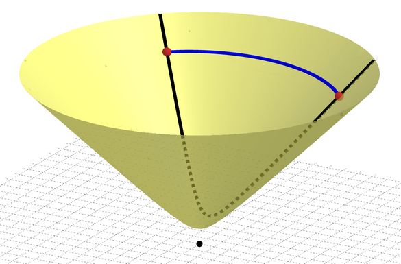
(a) Hyperboloid

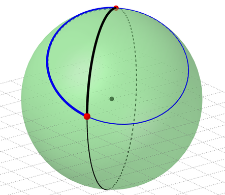
(b) Sphere

Figure 4: The hyperboloid model of hyperbolic geometry (left) and the spherical model of elliptical geometry (right). The black curves are geodesics between two points while the blue ones are arbitrary paths connecting them (not geodesics). Note that the ambient space of the hyperboloid is the Minkowski space, hence our Euclidean intuition does not apply, as it does for the sphere.

Appendix C Geometric Properties of Graphs

Graphs and manifolds, while different mathematical abstractions, share many similar properties through Laplace operators, heat kernels, and random walks. Another example is the deep connection between trees and the hyperbolic plane: any tree can be embedded in $\mathbb{H}(2)$ with arbitrarily small distortion [65]. On a similar note, complex networks arise naturally from hyperbolic geometry [44]. With these insights in mind, in this section we review some continuous geometric properties that have been adapted to arbitrary weighted graphs. See also [54].

Gromov Hyperbolicity.

Also known as $\delta$-hyperbolicity [34], it quantifies with a single number the hyperbolicity of a given metric space: the smaller $\delta$ is, the more hyperbolic-like or negatively-curved the space is. The definition that makes it easier to picture it is via the slim triangles property: a metric space $(M,d_{M})$ is $\delta$-hyperbolic if all geodesic triangles are $\delta$-slim. Three points $x,y,w\in M$ form a $\delta$-slim triangle if any point on the geodesic segment between any two of them is within distance $\delta$ from the other two geodesics (i.e., “sides” of the geodesic triangle).

For discrete metric spaces such as graphs, an equivalent definition using the so-called “4-points condition” can be used to devise algorithms that look at quadruples of points. Both exact and approximating algorithms exist that run fast enough to analyze graphs with tens of thousands of nodes within minutes [28, 19]. In practice we look at histograms of $\delta$ instead of the worst-case value.

Ollivier-Ricci Curvature.

Ollivier et al. [58] generalized the Ricci curvature to metric spaces $(M,d_{M})$ equipped with a family of probability measures $\{m_{x}(\cdot)\}_{x\in M}$. It is defined in a way that mimics the interpretation of Ricci curvature on Riemannian manifolds: it is the average distance between two small balls taken relative to the distance between their centers. The difference is that now the former is given by the Wasserstein distance (i.e., Earth mover’s distance) between the corresponding probability measures,

$$\overline{\operatorname{\mathrm{Ric}}}_{1}(x,y)\vcentcolon=1-\frac{W(m_{x},m_{y})}{d_{M}(x,y)},$$ (25)

with $W(\mu_{1},\mu_{2})\vcentcolon=\inf_{\xi}\int_{x}\int_{y}d(x,y)d\xi(x,y)$ and $\xi(x,y)$ – a join distribution with marginals $\mu_{1}$ and $\mu_{2}$. This definition was then specialized in [51] for graphs by making $m_{x}$ assign a probability mass of $\alpha\in[0,1)$ to itself (node $x$) and spread the remaining $1-\alpha$ uniformly across its neighbors. They refer to $\overline{\operatorname{\mathrm{Ric}}}_{\alpha}(x,y)\vcentcolon=\overline{\operatorname{\mathrm{Ric}}}_{1}(x,y)$ as the $\alpha$-Ricci curvature and define instead

$$\overline{\operatorname{\mathrm{Ric}}}_{2}(x,y)\vcentcolon=\lim_{\alpha\to 1}\frac{\overline{\operatorname{\mathrm{Ric}}}_{\alpha}(x,y)}{1-\alpha}$$ (26)

to be the Ricci curvature of edge $(x,y)$ in the graph. In practice, we approximate the limit via a large $\alpha$, e.g., $\alpha=0.999$.

Notice that in contrast to $\delta$-hyperbolicity, the Ricci curvature characterizes the space only locally. It yields the curvatures one would expect in several cases: negative curvatures for trees (except for the edges connecting the leaves) and positive for complete graphs and hypercubes; but it does not capture the curvature of a cycle with more than 5 nodes because it locally looks like a straight line.

Sectional Curvatures.

A discrete analogue of sectional curvature for graphs is obtained as the deviation from the parallelogram law in Euclidean geometry [36]. It uses the same intuition as before: in non-positively curved spaces triangles are “slimmer” while in non-negatively curved ones they are “thicker” (see Figure 5).

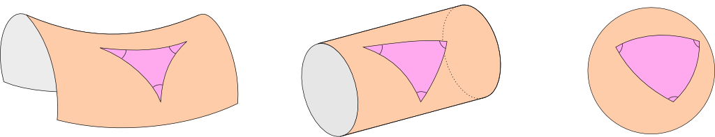
Figure 5: Geodesic triangles in negatively curved, flat, and positively curved spaces, respectively. Source: www.science4all.org

For any Riemannian manifold $\mathcal{M}$, let $x,y,z\in\mathcal{M}$ form a geodesic triangle, and let $m$ be the midpoint of the geodesic between $y$ and $z$. Then, the following quantity

$$k_{\mathcal{M}}(x,y,z)\vcentcolon=d_{\mathcal{M}}(x,m)^{2}+d_{\mathcal{M}}(y,z)^{2}/4-\big{(}d_{\mathcal{M}}(x,y)^{2}+d_{\mathcal{M}}(x,z)^{2}\big{)}/2$$ (27)

has the same sign as the sectional curvatures in $\mathcal{M}$ and it is identically zero if $\mathcal{M}$ is flat. For a graph $G=(V,E)$, an analogue is defined for each node $m$ and two neighbors $y$ and $z$, as

$$k_{G}(m;y,z;x)=\frac{1}{2d_{G}(x,m)}k_{G}(x,y,z).$$ (28)

With that, the sectional curvature of the graph $G$ at $m$ in “directions” $y$ and $z$ is defined as the average of (28) across all $x\in G$,

$$k_{G}(m;y,z)=\frac{1}{\lvert V\rvert-1}\sum_{x\neq m}k_{G}(m;y,z;x).$$ (29)

It is also shown in [36, AppxC.2] that this definition recovers the expected signs for trees (negative or zero), cycles (positive or zero) and lines (zero).

Appendix D Matrix Manifolds – Details

In this section, we include several results that are useful for better understanding and working with the matrix manifolds introduced in Section 3. They have been left out from the main text due to space constraints. Furthermore, we describe the orthogonal group $O(n)$ which is used in our random manifold graphs analysis from Appendix E. We do not use it for graph embedding purposes in this work because its corresponding distance function does not immediately lend itself to simple backpropagation-based training (in general). This is left for future work.

Homogeneity.

It is a common property of the matrix manifolds used in this work. Formally, it means that the isometry group of $\mathcal{M}$ acts transitively: for any $A,B\in\mathcal{M}$ there is an isometry that maps $A$ to $B$. In non-technical terms this says that $\mathcal{M}$ “looks locally the same” around each point. A consequence of homogeneity is that in order to prove curvature properties, it suffices to do so at a single point, e.g., the identity matrix for $\mathcal{S}^{\texttt{++}}(n)$.

D.1 SPD Manifold

The following theorem, proved here for completeness, states that $\mathcal{S}^{\texttt{++}}(n)$ is a differentiable manifold.

Theorem 1.

The set $\mathcal{S}^{\texttt{++}}(n)$ of symmetric positive-definite matrices is an $\frac{n(n+1)}{2}$-dimensional differentiable manifold.

Proof.

The set $\mathcal{S}(n)$ is an $\frac{n(n+1)}{2}$-dimensional vector space. Any finite dimensional vector space is a differentiable manifold: fix a basis and use it as a global chart mapping points to the Euclidean space with the same dimension.

The set $\mathcal{S}^{\texttt{++}}(n)$ is an open subset of $\mathcal{S}(n)$. This follows from $(A,v)\mapsto v^{\top}Av$ being a continuous function. The fact that open subsets of (differentiable) manifolds are (differentiable) manifolds concludes the proof. $\square$

The following result from linear algebra makes it easier to compute geodesic distances.

Lemma 2.

Let $A,B\in\mathcal{S}^{\texttt{++}}(n)$. Then $AB$ and $A^{1/2}BA^{1/2}$ have the same eigenvalues.

Proof.

Let $A=A^{1/2}A^{1/2}$, where $A^{1/2}$ is the unique square root of $A$. Note that $A^{1/2}$ is itself symmetric and positive-definite because every analytic function $f(A)$ is equivalent to $U\operatorname{\mathop{\mathrm{diag}}}(\{f(\lambda_{i})\}_{i})U^{\top}$, where $A=U\operatorname{\mathop{\mathrm{diag}}}(\{\lambda_{i}\}_{i})U^{\top}$ is the eigenvalue decomposition of $A$, and $\lambda_{i}>0$ for all $i$ from positive-definiteness. Then, we have

$$AB=A^{1/2}A^{1/2}B=A^{1/2}(A^{1/2}BA^{1/2})A^{-1/2},$$

Therefore, $AB$ and $A^{1/2}BA^{1/2}$ are similar matrices so they have the same eigenvalues. $\square$

This is useful from a computational perspective because $A^{-1/2}BA^{-1/2}$ is an SPD matrix while $A^{-1}B$ may not even be symmetric. It also makes it easier to see the following equivalence, for any matrix $A\in\mathcal{S}^{\texttt{++}}(n)$:

$$\lVert\log(A)\rVert_{F}=\left\lVert U\operatorname{\mathop{\mathrm{diag}}}\Big{(}\log(\lambda_{i}(A))\Big{)}U^{T}\right\rVert_{F}=\left\lVert\operatorname{\mathop{\mathrm{diag}}}\Big{(}\log(\lambda_{i}(A))\Big{)}\right\rVert_{F}=\sqrt{\sum_{i=1}^{n}\log^{2}\big{(}\lambda_{i}(A)\big{)}},$$ (30)

where the first step decomposes the principle logarithm of $A$ and the second one uses the change of basis invariance of the Frobenius norm.

An even better behaved matrix that has the same spectrum and avoids matrix square roots altogether is $LBL^{\top}$, where $LL^{\top}$ is the Cholesky decomposition of $A$. Note that for the Stein divergence, the log-determinants can be computed in terms of $L$ as $\log\det(A)=2\sum_{i=1}^{n}\log(L_{ii})$.

An additional challenge with eigenvalue computations is that most linear algebra libraries are optimized for large matrices while our use-case involves milions of very small matrices. To overcome that, for $2\times 2$ and $3\times\ 3$ matrices we use custom formulas that can be derived explicitly:

• For $A\in\mathcal{S}^{\texttt{++}}(2)$, we have

  $$\lambda_{k}(A)=\frac{t}{2}\pm\sqrt{\bigg{(}\frac{t}{2}\bigg{)}^{2}-d},$$ (31)

  with $t=\operatorname{\mathop{\mathrm{Tr}}}A$ and $d=\det(A)$.

• For $A\in\mathcal{S}^{\texttt{++}}(3)$, we express it as an affine transformation of another matrix, i.e., $A=pB+q\operatorname{\mathop{\mathrm{Id}}}_{n}$. Then we have $\lambda_{k}(A)=p\lambda_{k}(B)+q$. Concretely, if we let

  $$q=\frac{\operatorname{\mathop{\mathrm{Tr}}}A}{3}\enskip\text{and}\enskip p=\sqrt{\frac{\operatorname{\mathop{\mathrm{Tr}}}\ (A-q\operatorname{\mathop{\mathrm{Id}}}_{n})^{2}}{6}},$$

  then the eigenvalues of $B$ are

  $$\lambda_{k}(B)=2\cos\bigg{(}\frac{1}{3}\arccos\Big{(}\frac{\det(B)}{2}\Big{)}+\frac{2k\pi}{3}\bigg{)}.$$ (32)

D.2 Grassmann Manifold

The following singular value formulas are useful in computing geodesic distances (1) between points on $Gr(2,n)$.

Proposition 3.

The singular values of $A=\begin{bmatrix}a&b\\ c&d\end{bmatrix}$ are

$$\sigma_{1}=\sqrt{\frac{S_{1}+S_{2}}{2}}\enskip\text{and}\enskip\sigma_{2}=\sqrt{\frac{S_{1}-S_{2}}{2}},$$

with

$$S_{1}=a^{2}+b^{2}+c^{2}+d^{2}\enskip\text{and}\enskip S_{2}=\sqrt{(a^{2}+b^{2}-c^{2}-d^{2})^{2}+4(ac+bd)^{2}}.$$

D.3 Orthogonal Group

It is defined as the set of $n\times n$ real orthogonal matrices,

$$O(n)\vcentcolon=\{A\in\mathbb{R}^{n\times n}:A^{\top}A=AA^{\top}=\operatorname{\mathop{\mathrm{Id}}}_{n}\}.$$ (33)

We are interested in the geometry of $O(n)$ rather than its group properties. Formally, this means that in what follows we describe its so-called principal homogeneous space, the special Stiefel manifold $V(n,n)$, rather than the group $O(n)$.

Theorem 4.

$O(n)$ is an $\frac{n(n-1)}{2}$-dimensional differentiable manifold.

Proof.

Consider the map $F:\mathbb{R}^{n\times n}\rightarrow\mathcal{S}(n),\ F(A)=A^{\top}A-\operatorname{\mathop{\mathrm{Id}}}_{n}$. It is clear that $O(n)=F^{-1}(\mathbf{0})$. The differential at $A$, $\operatorname{\textrm{D}}F(A)[B]=A^{\top}B+B^{\top}A$, is onto the space of symmetric matrices as a function of the direction $B\in\mathbb{R}^{n\times n}$, as shown by the fact that $\operatorname{\textrm{D}}F(A)\Big{[}\frac{1}{2}AP\Big{]}=P$ for all $P\in\mathcal{S}(n)$. Therefore, $F(\cdot)$ is full rank and by the submersion theorem (Appendix A) the orthogonal group is a differentiable (sub-)manifold. Its dimension is $d=\dim(\mathbb{R}^{n\times n})-\dim(\mathcal{S}(n))=n(n-1)/2$. $\square$

As a Riemannian manifold, $O(n)$ inherits the metric structure from the ambient space and thus the Riemannian metric is simply the Frobenius inner product,

$$\langle P,Q\rangle_{A}=\operatorname{\mathop{\mathrm{Tr}}}P^{\top}Q.$$ (34)

for $A\in O(n)$ and $P,Q\in T_{A}O(n)$. To derive its tangent space, we use the following general result.

Proposition 5 ([1]).

If $\mathcal{M}$ is an embedded submanifold of a vector space $\mathcal{E}$, defined as a level set of a constant-rank function $F:\mathcal{E}\rightarrow\mathbb{R}^{n}$, we have

$$T_{x}\mathcal{M}=\operatorname{\mathop{ker}}(\operatorname{\textrm{D}}F(x)).$$

Differentiating $A^{\top}A=\operatorname{\mathop{\mathrm{Id}}}_{n}$ yields $\dot{A}^{\top}A+A^{\top}\dot{A}=\mathbf{0}$ so the tangent space at $A$ is

$$T_{A}O(n)=\{P\in\mathbb{R}^{n\times n}:A^{\top}P=X\in\mathcal{S}_{skew}(n)\}=A\,\mathcal{S}_{skew}(n),$$ (35)

where $\mathcal{S}_{skew}(n)$ is the space of $n\times n$ skew-symmetric matrices.

Many Riemannian quantities of interest are syntactically very similar to those for the canonical SPD manifold (see Table 1). The connection is made precise by the following property.

Lemma 6 ([25]).

The metric (34) is the opposite of the affine-invariant metric (1) that the SPD manifold is endowed with.

Proof.

Let $A\in O(n)$ and $P_{1},P_{2}\in T_{A}O(n)$. Then,

$$\operatorname{\mathop{\mathrm{Tr}}}A^{-1}P_{1}A^{-1}P_{2} =\operatorname{\mathop{\mathrm{Tr}}}A^{\top}AX_{1}A^{\top}AX_{2}=\operatorname{\mathop{\mathrm{Tr}}}X_{1}X_{2} P_{i}=AX_{i}$$ ()

$$=-\operatorname{\mathop{\mathrm{Tr}}}X_{1}^{\top}X_{2}=-\operatorname{\mathop{\mathrm{Tr}}}\ (AX_{1})^{\top}(AX_{2}) X_{i}\in\mathcal{S}_{skew}(n)$$ ()

$$=-\operatorname{\mathop{\mathrm{Tr}}}P_{1}^{\top}P_{2}.$$

$\square$

An important characteristic of $O(n)$ is its compact Lie group structure which implies, via the Hopf-Rinow theorem, that its components (see below) are geodesically complete: all geodesics $t\mapsto A\exp(tA^{\top}P)$ are defined on the whole real line. Note, though, that they are minimizing only up to some $t_{0}\in\mathbb{R}$. This is another consequence of its compactness.

Moreover, $O(n)$ has two connected components so the expression for the geodesic between two matrices $A,B\in O(n)$,

$$\gamma_{A,B}(t)=A(A^{\top}B)^{t},$$ (36)

only makes sense if they belong to the same component. The same is true for the logarithm map,

$$\log_{A}(B)=A\log(A^{\top}B).$$ (37)

The two components contain the orthogonal matrices with determinant $1$ and $-1$, respectively. The former is the so-called special orthogonal group,

$$SO(n)\vcentcolon=\{A\in O(n):\det(A)=1\}.$$ (38)

Restricting to one of them guarantees that the logarithm map is defined on the whole manifold except for the cut locus (see Appendix A). This is true in general for compact connected Lie groups endowed with bi-invariant exponential maps, but we can bring it down to a clearer matrix property by looking at its expression,

$$d(A,B)=\lVert\log(A^{\top}B)\rVert_{F}.$$ (39)

Notice that $A^{\top}B$ is in $SO(n)$ whenever $A$ and $B$ belong to the same component,

$$\det(A)=\det(B)=d\in\{-1,1\}\implies\det(A^{\top}B)=1.$$ (40)

Then, the claim is true due the surjectivity of the matrix exponential, as follows.

Proposition 7 ([15]).

For any matrix $A\in SO(n)$, there exists a matrix $X\in\mathcal{S}_{skew}(n)$ such that $\exp(X)=A$, or, equivalently, $\log(A)=X$. Moreover, if $A$ has no negative eigenvalues, there is a unique such matrix with $\mathop{\mathrm{Im}}\lambda_{i}(X)\in(-\pi,\pi)$, called its principal logarithm.

This property makes it easier to see that the cut locus at a point $A\in SO(n)$ consists of those matrices $B\in SO(n)$ such that $A^{\top}B$ has eigenvalues equal to $-1$. They can be thought of as analogous to the antipodal points on the sphere. It also implies that the distance function (39), expanded as

$$d(A,B)=\lVert\log(A^{\top}B)\rVert_{F}=\sqrt{\sum_{i=1}^{n}\operatorname{\mathop{\mathrm{Arg}}}\big{(}\lambda_{i}(A^{\top}B)\big{)}^{2}},$$ (41)

is well-defined for points in the same connected components. The $\operatorname{\mathop{\mathrm{Arg}}}(\cdot)$ operator denotes the complex argument. Notice again the similarity to the canonical SPD distance (1). However, the nicely behaved symmetric eigenvalue decomposition cannot be used anymore and the various approximations to the matrix logarithm are too slow for our graph embedding purposes. That is why we limit our graph reconstruction experiments with compact matrix manifolds to the Grassmann manifold. Moreover, the small dimensional cases where we could compute the complex argument “manually” are isometric to other manifolds that we experiment with: $O(2)\cong\mathbb{S}(1)$ and $O(3)\cong Gr(1,4)$.

Appendix E Manifold Random Graphs

The idea of sampling points on the manifolds of interest and constructing nearest-neighbor graphs, used in prior influential works such as [44], is motivated, in our case, by the otherwise black-box nature of matrix embeddings. However, in Section 5 we do not stop at reporting reconstruction metrics, but look into manifold properties around the embeddings. But even with that, the discretization of the embedding spaces is a natural first step in developing an intuition for them.

The discretization is achieved as follows: several samples ($1000$ in our case) are generated randomly on the target manifold and a graph is constructed by linking two nodes together (corresponding to two sample points) when the geodesic distance between them is less than some threshold. The details of the random generation is discussed in each of the following two subsections. As mentioned in the introductory paragraph, it is the same approach employed in [44] who sample from the hyperbolic plane and obtain graphs that resemble complex networks. In our experiments, we go beyond their technique and study the properties of the generated graphs when varying the distance threshold.

E.1 Compact Matrix Manifolds vs. Sphere

We begin the analysis of random manifold graphs with the compact matrix manifolds compared against the elliptical geometry. The sampling is performed uniformly on each of the compact spaces.

The results are shown in Figure 6. The node degrees and the graph sectional curvatures (computed via the “deviation from parallelogram law”; see Appendix C) are on the first two rows. The markers are the median values and the shaded area corresponds to the inter-quartile range (IQR). The last row shows normalized sum-of-angles histograms. All of them are repeated for three consecutive dimensions, organized column-wise. The distance thresholds used to link nodes in the graph range from $d_{\textrm{max}}/10$ to $d_{\textrm{max}}$, where $d_{\textrm{max}}$ is the maximum distance between any two sample points, for each instance except for the Euclidean baseline which uses the maximum distance across all manifolds (i.e., $\approx 4.4$ corresponding to $SO(3)$).

Degree Distributions.

From the degree distributions, we first notice that all compact manifolds lead to graphs with higher degrees for the same distance threshold than the ones based on uniform samples from Euclidean balls. This is not surprising given that points tend to be closer due to positive curvature. Furthermore, the distributions are concentrated around the median – the IQRs are hardly visible. To get more manifold-specific, we see that Grassmannians lead to full cliques faster than the spherical geometry, but the curves get closer and closer as the dimension is increased. This is the same behavior that in Euclidean space is known as the “curse of dimensionality”, i.e., a small threshold change takes us from a disconnected graph to a fully-connected one. For the compact manifolds, though, this can be noticed already at a very small dimension: the degree distributions tend towards a step function. The only difference is the point where that happens, which depends on the maximum distance on each manifold. For instance, that is much earlier on the real projective space $\mathbf{RP}(n-1)\cong Gr(1,n)$ than the special orthogonal group $SO(n)$.

Graph Sectional Curvatures.

They confirm the similarity between the compact manifolds that we have just hinted at: for each of the three dimensions, the curves look almost identical up to a frequency change (i.e., “stretching them”). We say “almost” because we can still see certain differences between them (explained by the different geometries); for instance, in Figure 6f, the graph curvatures corresponding to Grassmann manifolds are slightly larger at distance threshold $\approx 1$. This frequency change seems to be intimately related to the injectivity radii of the manifolds [see, e.g., 72]. We also see that distributions are mostly positive, matching their continuous analogues. A-priori, it is unclear if manifold discretization will preserve them. Finally, the convergence point is $k_{G}(m;x,y)=1/8$ – the constant sectional curvature of a complete graph (see eqs. 27 and 28).

Triangles Thickness.

The normalized sum-of-angles plots do not depend on the generated graphs: the geodesic triangles are randomly selected from the manifold-sampled points. As a sanity check, we first point out that they are all positive. We observe that the Grassmann samples yield empirical distributions that look bi-modal. At the same time, the elliptical ones result in normalized sum-of-angles that resemble Poisson distributions, with the dimension playing the role of the parameter $\lambda$. We could not justify these contrasting behaviors, but they show that the spaces curve differently. What we can justify is the perfect overlap of the distributions corresponding to $SO(3)$ and $Gr(1,4)$ in Figure 6h: the two manifolds are isometric. The seemingly different degree distributions from Figure 6b should, in fact, be identical after a rescaling. In other words, they have different volumes but curve in the same way.

(a) node degrees; $n=2$

(b) node degrees; $n=3$

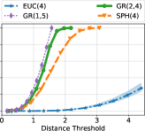
(c) node degrees; $n=4$

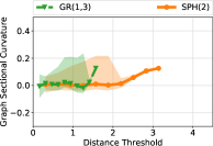
(d) graph sec. curv.; $n=2$

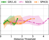
(e) graph sec. curv.; $n=3$

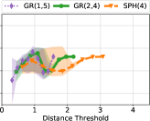
(f) graph sec. curv.; $n=4$

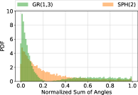
(g) man. angles; $n=2$

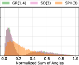
(h) man. angles; $n=3$

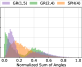
(i) man. angles; $n=4$

Figure 6: Analysis of graphs sampled from the compact manifolds. The results are grouped by manifold dimension (one column each). The first row (a)-(c) shows the node distributions as the distance threshold used to link two nodes is varied. Samples from an Euclidean ball of radius $4.4$ are included for comparison. The shaded range, hardly noticeable for compact manifolds, is the IQR. The second row (d)-(f), with the same $x$-axis as the first one, shows the distributions of graph sectional curvatures obtained via the deviation from parallelogram law (see Appendix C). The third row (g)-(i) shows histograms of normalized angle sums obtained from manifold-sampled triangles. It does not depend on the graphs analyzed in the previous plots but only on the manifold samples.

E.2 SPD vs. Hyperbolic vs. Euclidean

In this subsection, using the same framework as for compact manifolds, we compare the non-positively curved manifold of positive-definite matrices to hyperbolic and Euclidean spaces.

A Word on Uniform Sampling.

Ideally, to follow [44] and to recover their results, we would have to sample uniformly from geodesic balls of some fixed radius. However, this is non-trivial for arbitrary Riemannian manifolds and, in particular, to the best of our knowledge, for the SPD manifold. One would have to sample from the corresponding Riemannian measure while enforcing the maximum distance constraint given by the geodesic ball. More precisely, using the following formula for the measure $\mathrm{d}\mu_{g}$ in terms of the Riemannian metric $g(x)$, expressed in a normal coordinates system $x$ [see, e.g., 60]

$$\mathrm{d}\mu_{g}=\sqrt{\det g(x)}\ \mathrm{d}^{n}x,$$ (42)

one can sample uniformly with, for instance, a rejection sampling algorithm, as long as the right hand side can be computed and the parametrization allows enforcing the support constraint. This is possible for hyperbolic and elliptical spaces through their polar parametrizations. In spite of our efforts, we have not managed to devise a similar procedure for the SPD manifold. Instead, we have chosen a non-uniform sampling approach, applied consistently, which first generates uniform tangent vectors from a ball in the tangent space at some point and then maps them onto the manifold via the exponential map. Note that the manifold homogeneity guarantees that we get the same results irrespective of the chosen base point, so in our experiments we sample around the identity matrix. The difference from the uniform distribution is visualized in Figure 7 for $\mathbb{H}(3)$ and $\mathbb{S}(2)$.

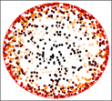
(a) $\mathbb{H}(3)$ – uniform

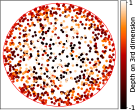
(b) $\mathbb{H}(3)$ – exp map

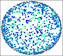
(c) $\mathbb{S}(2)$ – uniform

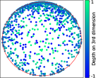
(d) $\mathbb{S}(2)$ – exp map

Figure 7: Visualization of the bias incurred when sampling through the exponential map. For the $3$-dimensional Poincaré ball (left), uniform samples (from a geodesic ball of radius $5$) are more concentrated towards the boundary. The bias is even more apparent for the $2$-dimensional sphere (right), where sampling through the exponential map at the south pole, in a ball of radius $\pi$, yields too many samples around the north pole. That is because the curvature is not taken into account.

With that, we proceed to discussing the results from Figure 8. They are organized as in the previous subsection. One difference, besides the sampling procedure, is that we now vary the distance threshold used to link nodes in the graphs from $R/10$ to $1.5R$, where $R$ is the radius of the geodesic balls (i.e., half of the maximum distance between any two points). It is identically $5$ in all scenarios.

Degree Distributions.

The first obvious characteristic is that the Euclidean space now bounds from above the two non-flat manifolds (that is, their corresponding median curves). Contrast this with the compact manifolds (Figure 6). It tells us that points are in general farther away than the others (relative to the Euclidean space), which is expected, given their (partly) negative curvature. Moreover, recall that the SPD manifold is a higher-rank symmetric space, which means that there are tangent space subspaces with dimension greater than 1 on which the sectional curvature is 0. In light of this property, its interpolating behavior (of Euclidean and Hyperbolic curves), which is already apparent from the evolution of the degree distribution, is not surprising. Note that in $10$ dimensions, the graphs constructed from the hyperbolic space are poorly connected even for the higher end of the threshold range. A similar trend characterizes the Euclidean and SPD spaces, but at a lower rate. In the limit $n\to\infty$, essentially all the mass is at the boundary of the geodesic ball for all of them, but how quickly this happens is what distinguishes them.

Graph Sectional Curvatures.

Here, the difference between the three spaces is hardly noticeable for $n=3$, in Figure 8d, but it becomes clearer in higher dimensions. We see that as long as the graphs are below a certain median degree, the estimated discrete curvatures are mostly negative, as one would expect. Furthermore, the order of the empirical distributions seems to match the intuition built in the previous paragraph: the hyperbolic space is “more negatively curved” than the SPD manifold.

Triangles Thickness.

The last row in Figure 8 serves as additional evidence that the SPD manifold is not “as negatively curved” as the hyperbolic space. Without any further comments, we need only emphasize that, as the dimension increases, almost all hyperbolic triangles are “ideal triangles”, i.e., the largest possible triangles in hyperbolic geometry, with the sum-of-angles equal to 0. The analogous histograms for the SPD manifold shift and peak slightly to the left but at a much slower pace.

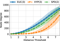
(a) node degrees; $n=3$

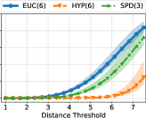
(b) node degrees; $n=6$

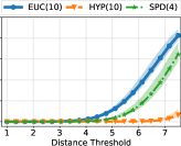
(c) node degrees; $n=10$

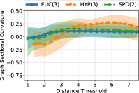
(d) graph sec. curv.; $n=3$

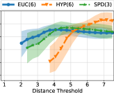
(e) graph sec. curv.; $n=6$

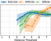
(f) graph sec. curv.; $n=10$

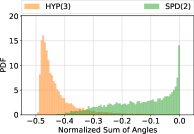
(g) man. angles; $n=3$

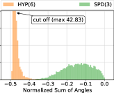
(h) man. angles; $n=6$

(i) man. angles; $n=10$

Figure 8: Analysis of graphs sampled from geodesic balls in $\mathbb{R}^{n}$, $\mathbb{H}(n)$, and $\mathcal{S}^{\texttt{++}}(n)$. The plots follow the same organization as in Figure 6. The points are obtained by sampling tangent vectors from a ball of radius $5$, uniformly, and mapping them onto the manifold through the exponential map. A few points are missing from the second set of plots because the largest connected components in the corresponding graphs have too few nodes (less than 100).

Appendix F Experimental Setup

The training procedure is the same across all the experiments from Section 5. The structure of the input graphs is not altered. We compute all-pairs shortest-paths in each one of the input graphs and serialize them to disk. They can then be reused throughout our experiments. Since we are not interested in representing the distances exactly (in absolute value) but only relatively, we max-scale them. This has the (empirically observed) advantage of making learning less sensitive to the scaling factors (see below).

The Task.

We emphasize that we consider the graph reconstruction task in Section 5. Hence, all results correspond to embedding the input graphs containing all information: no edges or nodes are left out. In other words, we do not evaluate generalization. That is why for each embedding space and fixed dimension, we report the best performing embedding across all runs and loss functions. This is consistent with our goal of decoupling learning objectives and evaluation metrics (see Section 4). We have chosen to restrict our focus as such in order to have fewer factors in our ablation studies. As future work, it is natural to extend our work to downstream tasks and generalization-based scenarios, and study the properties of the introduced matrix manifolds in those settings.

Training.

We train for a maximum of 3000 epochs with batches of 512 nodes – that is, 130816 pairwise distances. We use the burn-in strategy from [55, 29]: training with a 10 times smaller learning rate for the first 10 epochs. Moreover, if the per-epoch loss does not improve for more than 50 epochs, we decrease the learning rate by a factor of 10; the training is ended earlier if this makes the learning rate smaller than $10^{-5}$. This saves time without affecting performance.

Optimization.

We repeat the training, as described so far, for three optimization settings. The first one uses Radam [4] to learn the embeddings, which we have seen to be the most consistent across our early experiments. In the other two, we train the embeddings using Rsgd and Radam, respectively, but we also train a scaling factor of pairwise distances (with the same optimizer). This is inspired by [36]. The idea is that scaling the distance function is equivalent to representing the points on a more or less curved sphere or hyperboloid. In the spirit of Riemannian SNE (Section 4), this can also be seen as controlling how peaked around the MAP configuration the resulting distribution should be. We have chosen to optimize without scaling in the first setting because it seemed that even for simple, synthetic examples, jointly learning the scaling factor is challenging.

We have also experimented with an optimization inspired by deterministic annealing [62]: starting with a high “temperature” and progressively cooling it down. Since we did not see significant improvements, we did not systematically employ this approach.

Computing Infrastructure.

We used 4 NVIDIA GeForce GTX 1080 Ti GPUs for the data-parallelizable parts.

Appendix G Input Graphs – Properties & Visualizations

First of all, we include a visualization of each one of the graph used throughout our graph reconstruction experiments in Figure 10. In the rest of this section, we look at some of their geometric properties, summarized in Figure 9. We refer the reader to Appendix C for background on the quantities discussed next.

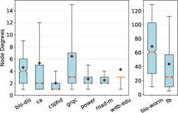
(a)

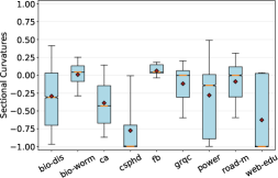
(b)

	bio-dis	bio-worm	ca	csphd	fb	grqc	power	road-m	web-edu
$\delta$-mean	$0.20$	$0.24$	$0.31$	$0.51$	$0.10$	$0.38$	$0.96$	$3.13$	$0.02$
$\delta$-max	$2.50$	$2.00$	$2.50$	$6.50$	$1.50$	$3.00$	$10.00$	$25.00$	$1.00$

Figure 9: The node degrees, (graph) sectional curvatures, and $\delta$-hyperbolicities (including the mean of the empirical distribution sampled as shown in [19]) of the input graphs used throughout our experiments with non-positively curved manifolds. Shortened dataset names are used to save space.

We start with node degree distributions. Judging by the positions of the means (red diamonds) relative to those of the medians (orange lines), we conclude that most degree distributions are long-tailed, a feature of complex networks. This is particularly severe for “web-edu”, where the mean degree is larger than the 90th percentile. Looking at Figure 1a, it becomes clear what makes it so: there are a few nodes (i.e., web pages) to which almost all the others are connected.

Next, we turn to the estimated sectional curvatures. They indicate a preference for the negative half of the range, reinforcing the complex network resemblance. We see that many of the distributions resemble those of the random graphs sampled from hyperbolic and SPD manifolds (Figures 8e and 8f).

Finally, with one exception, the graphs are close to $0$ hyperbolicity, which is an additional indicator of a preference for negative curvature; but how much negative curvature is beneficial remains, a-priori, unclear. The exception is “road-minnesota” which, as its name implies, is a road network and, unsurprisingly, has a different geometry than the others. Its $\delta$-hyperbolicity values are mostly large, an indicator of thick triangles and, hence, positive curvature, as discussed in Appendix C.

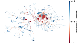
(a) “bio-diseasome” ($\lvert V\rvert=516,\lvert E\rvert=1188$) – disorder-gene associations [33]

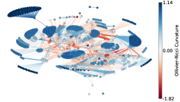
(b) “bio-wormnet” ($\lvert V\rvert=2274,\lvert E\rvert=78328$) – worms gene network [17]

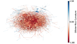
(c) “california” ($\lvert V\rvert=5925,\lvert E\rvert=15770$) – [63]

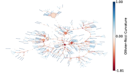
(d) “csphd” ($\lvert V\rvert=1025,\lvert E\rvert=1043$) – scientific collaboration network [21]

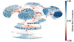
(e) “facebook” ($\lvert V\rvert=4039,\lvert E\rvert=88234$) – dense social network from Facebook [48]

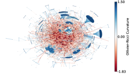
(f) “grqc” ($\lvert V\rvert=4158,\lvert E\rvert=13422$) – collaboration network on “General Relativity” [47]

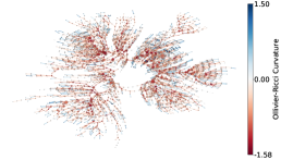
(g) “power” ($\lvert V\rvert=4941,\lvert E\rvert=6594$) – grid distribution network [76]

Figure 10: Visualizations of embedded graphs. The edge color depicts the corresponding Ollivier-Ricci curvature, as described in Appendix C. Similarly, each node is colored according to the average curvature of its adjacent edges. Thus, red nodes behave more like backbone nodes, while blue nodes are either leaves or are part of a clique. In each plot, the size of each node is proportional to its degree.

Appendix H Extended Graph Reconstruction Results

$\mathcal{S}^{\texttt{++}}$ vs. $\mathbb{H}$.

All graph reconstruction results comparing the SPD and hyperbolic manifolds are shown in Table 5. Compared to Table 2 from the main text this table includes, on one hand, more graphs and, at the same time, the performance results on 10-dimensional manifolds for most datasets. Notice, in particular, that the results for two much larger graphs are included [47]: “cit-dblp” and “condmat”. They are both citation networks with about 12000 and 23000 nodes, respectively. The columns are the same as in Table 2.

$Gr$ vs. $\mathbb{S}$.

All graph reconstruction results comparing the Grassmann and spherical manifolds are shown in Table 6. It includes two 3D models from the Stanford 3D Scanning Repository [49]: the notorious “Stanford bunny” and a “drill shaft” (the mesh of a drill bit).

Cartesian Products.

Graph reconstruction results comparing several product manifolds are shown in Table 7. The three datasets were chosen as some of the most challenging based on the previous results. The SPD embeddings are trained using the Stein divergence. All six product manifolds have 12 free parameters.

Table 5: All graph reconstruction results for “$\mathcal{S}^{\texttt{++}}$ vs. $\mathbb{H}$”. See text for more details.

$G$	$n$	$\mathcal{M}$	F1@1	AUC	AD
bio-diseasome	3	Euc	83.78	91.21	0.145
		Hyp	86.21	95.72	0.137
		SPD	83.99	91.32	0.140
		Stein	86.70	94.54	0.105
	6	Euc	93.48	95.84	0.073
		Hyp	96.50	98.42	0.071
		SPD	93.83	95.93	0.072
		Stein	94.86	97.64	0.066
bio-wormnet	3	Euc	89.36	93.84	0.157
		Hyp	91.26	97.01	0.157
		SPD	88.91	94.36	0.159
		Stein	90.92	95.80	0.120
	6	Euc	98.14	97.89	0.090
		Hyp	98.55	99.00	0.089
		SPD	98.12	97.90	0.090
		Stein	98.29	98.63	0.085
california	3	Euc	15.97	77.99	0.2297
		Hyp	29.72	85.78	0.109
		SPD	15.61	82.82	0.230
		Stein	24.66	84.04	0.118
	6	Euc	29.29	84.59	0.143
		Hyp	43.04	88.64	0.098
		SPD	29.20	86.30	0.122
		Stein	34.85	87.95	0.101
	10	Euc	41.39	87.77	0.105
		Hyp	51.11	90.68	0.094
		SPD	41.81	90.10	0.098
		Stein	46.03	90.11	0.091
condmat	3	Euc	16.01	74.62	0.303
		Hyp	21.67	84.14	0.186
		SPD	16.63	80.66	0.303
	6	Euc	31.53	81.01	0.242
		Hyp	47.53	87.58	0.180
		SPD	32.31	83.04	0.200
power	3	Euc	49.34	87.84	0.119
		Hyp	60.18	91.28	0.068
		SPD	52.48	90.17	0.121
		Stein	54.06	90.16	0.076
	6	Euc	63.62	92.09	0.061
		Hyp	75.02	94.34	0.060
		SPD	67.69	91.76	0.062
		Stein	70.70	93.32	0.049
	10	Euc	74.14	94.35	0.042
		Hyp	84.77	96.25	0.038
		SPD	79.36	95.59	0.033
		Stein	78.13	94.67	0.040
road-minnesota	3	Euc	90.35	95.94	0.058
		Hyp	90.02	95.82	0.058
		SPD	89.71	95.94	0.058
		Stein	91.96	96.02	0.060
	6	Euc	96.68	97.21	0.045
		Hyp	96.59	97.17	0.046
		SPD	96.81	97.20	0.045
		Stein	96.21	97.20	0.046

$G$	$n$	$\mathcal{M}$	F1@1	AUC	AD
cit-dblp	3	Euc	11.43	79.63	0.311
		Hyp	20.05	86.97	0.199
		SPD	11.54	83.10	0.311
	6	Euc	24.38	85.32	0.253
		Hyp	34.79	89.80	0.205
		SPD	24.80	87.27	0.253
csphd	3	Euc	52.12	89.36	0.123
		Hyp	55.55	92.46	0.124
		SPD	52.34	89.71	0.127
		Stein	54.45	91.61	0.098
	6	Euc	60.63	93.91	0.065
		Hyp	64.89	94.73	0.065
		SPD	60.59	94.12	0.066
		Stein	62.73	94.95	0.062
	10	Euc	66.66	96.06	0.050
		Hyp	74.76	96.38	0.045
		SPD	67.46	96.34	0.048
		Stein	70.53	96.22	0.050
facebook	3	Euc	70.28	95.27	0.193
		Hyp	71.08	95.46	0.173
		SPD	71.09	95.26	0.170
		Stein	75.91	95.59	0.114
	6	Euc	79.60	96.41	0.090
		Hyp	81.83	96.53	0.089
		SPD	79.52	96.37	0.090
		Stein	83.95	96.74	0.061
	10	Euc	85.03	97.99	0.054
		Hyp	86.93	97.28	0.053
		SPD	85.25	97.98	0.049
		Stein	89.25	97.82	0.044
grqc	3	Euc	49.61	79.99	0.212
		Hyp	66.54	87.34	0.108
		SPD	50.41	80.48	0.208
		Stein	57.26	85.20	0.115
	6	Euc	71.71	86.89	0.125
		Hyp	82.43	91.53	0.091
		SPD	72.06	88.60	0.125
		Stein	78.00	90.20	0.094
	10	Euc	83.97	91.28	0.090
		Hyp	89.33	94.19	0.077
		SPD	84.74	93.48	0.081
		Stein	87.62	93.19	0.081
web-edu	3	Euc	29.18	87.14	0.245
		Hyp	55.60	92.10	0.245
		SPD	29.02	88.54	0.246
		Stein	48.28	90.87	0.084
	6	Euc	49.31	91.19	0.143
		Hyp	66.23	95.78	0.143
		SPD	42.16	91.90	0.142
		Stein	62.81	96.51	0.043
	10	Euc	42.47	93.31	0.082
		Hyp	98.43	98.18	0.073
		SPD	88.30	96.86	0.045
		Stein	91.02	98.24	0.037

Table 6: All graph reconstruction results for “$Gr$ vs. $\mathbb{S}$”. See text for more details.

$G$	$n$	$\mathcal{M}$	F1@1	AUC	AD
sphere-mesh	2	Sphere	99.99	98.31	0.051
		$Gr(1,3)$	97.20	90.66	0.148
	3	Sphere	100.00	98.76	0.042
		$Gr(1,4)$	100.00	98.38	0.060
	4	Sphere	100.00	98.84	0.041
		$Gr(1,5)$	100.00	98.69	0.060
		$Gr(2,4)$	100.00	98.94	0.040
bunny	2	Sphere	88.12	89.61	0.146
		$Gr(1,3)$	85.06	85.95	0.146
	3	Sphere	94.96	96.86	0.062
		$Gr(1,4)$	95.41	97.22	0.062
	4	Sphere	95.91	97.53	0.055
		$Gr(1,5)$	96.03	97.63	0.057
		$Gr(2,4)$	95.86	97.62	0.058
drill-shaft	2	Sphere	84.67	96.27	0.073
		$Gr(1,3)$	83.40	96.34	0.074
	3	Sphere	89.14	97.85	0.052
		$Gr(1,4)$	88.88	97.81	0.052
	4	Sphere	92.45	98.51	0.043
		$Gr(1,5)$	92.44	98.51	0.043
		$Gr(2,4)$	92.77	98.54	0.043
road-minnesota	2	Sphere	82.19	94.02	0.085
		$Gr(1,3)$	78.91	94.02	0.085
	3	Sphere	89.55	95.89	0.059
		$Gr(1,4)$	90.02	95.88	0.058
	4	Sphere	93.65	96.66	0.049
		$Gr(1,5)$	93.89	96.67	0.049
		$Gr(2,4)$	94.01	96.66	0.049
cat-cortex	2	Sphere	-	-	0.255
		$Gr(1,3)$	-	-	0.234
	3	Sphere	-	-	0.195
		$Gr(1,4)$	-	-	0.168
	4	Sphere	-	-	0.156
		$Gr(1,5)$	-	-	0.139
		$Gr(2,4)$	-	-	0.129

Table 7: Graph reconstruction results for six Cartesian products of Riemannian manifolds. See text for more details.

$G$	$\mathcal{M}$	F1@1	AUC	AD
california	$\mathbb{H}(3)^{4}$	55.15	91.35	0.096
	$\mathbb{H}(6)^{2}$	56.93	91.55	0.096
	$\mathbb{H}(6)\times\mathbb{S}(6)$	55.12	91.15	0.096
	$\mathcal{S}^{\texttt{++}}(2)^{4}$	49.49	90.77	0.087
	$\mathcal{S}^{\texttt{++}}(3)^{2}$	50.78	90.82	0.086
	$\mathcal{S}^{\texttt{++}}(3)\times Gr(3,5)$	47.21	90.53	0.089
grqc	$\mathbb{H}(3)^{4}$	92.03	95.06	0.081
	$\mathbb{H}(6)^{2}$	91.14	94.97	0.080
	$\mathbb{H}(6)\times\mathbb{S}(6)$	91.82	94.44	0.081
	$\mathcal{S}^{\texttt{++}}(2)^{4}$	89.39	94.25	0.080
	$\mathcal{S}^{\texttt{++}}(3)^{2}$	89.29	94.20	0.076
	$\mathcal{S}^{\texttt{++}}(3)\times Gr(3,5)$	89.54	93.79	0.081
web-edu	$\mathbb{H}(3)^{4}$	99.26	98.54	0.070
	$\mathbb{H}(6)^{2}$	98.62	99.24	0.071
	$\mathbb{H}(6)\times\mathbb{S}(6)$	99.14	98.39	0.071
	$\mathcal{S}^{\texttt{++}}(2)^{4}$	71.90	96.78	0.027
	$\mathcal{S}^{\texttt{++}}(3)^{2}$	78.47	97.12	0.027
	$\mathcal{S}^{\texttt{++}}(3)\times Gr(3,5)$	69.76	96.24	0.073

References

- [1] P-A Absil, Robert Mahony, and Rodolphe Sepulchre. Optimization algorithms on matrix manifolds. Princeton University Press, 2009.
- [2] Vincent Arsigny, Pierre Fillard, Xavier Pennec, and Nicholas Ayache. Log-euclidean metrics for fast and simple calculus on diffusion tensors. Magnetic Resonance in Medicine: An Official Journal of the International Society for Magnetic Resonance in Medicine, 56(2):411–421, 2006.
- [3] Gregor Bachmann, Gary Bécigneul, and Octavian-Eugen Ganea. Constant curvature graph convolutional networks. arXiv preprint arXiv:1911.05076, 2019.
- [4] Gary Becigneul and Octavian-Eugen Ganea. Riemannian adaptive optimization methods. In International Conference on Learning Representations, 2019.
- [5] Mikhail Belkin and Partha Niyogi. Laplacian eigenmaps and spectral techniques for embedding and clustering. In Advances in neural information processing systems, pages 585–591, 2002.
- [6] Yoshua Bengio, Aaron Courville, and Pascal Vincent. Representation learning: A review and new perspectives. IEEE transactions on pattern analysis and machine intelligence, 35(8):1798–1828, 2013.
- [7] Yoshua Bengio et al. Learning deep architectures for ai. Foundations and trends® in Machine Learning, 2(1):1–127, 2009.
- [8] Rajendra Bhatia. Positive definite matrices, volume 24. Princeton university press, 2009.
- [9] Rajendra Bhatia, Tanvi Jain, and Yongdo Lim. On the bures–wasserstein distance between positive definite matrices. Expositiones Mathematicae, 37(2):165–191, 2019.
- [10] Silvere Bonnabel. Stochastic gradient descent on riemannian manifolds. IEEE Transactions on Automatic Control, 58(9):2217–2229, 2013.
- [11] Martin R Bridson and André Haefliger. Metric spaces of non-positive curvature, volume 319. Springer Science & Business Media, 2013.
- [12] Alexander M Bronstein, Michael M Bronstein, and Ron Kimmel. Generalized multidimensional scaling: a framework for isometry-invariant partial surface matching. Proceedings of the National Academy of Sciences, 103(5):1168–1172, 2006.
- [13] Michael M Bronstein, Joan Bruna, Yann LeCun, Arthur Szlam, and Pierre Vandergheynst. Geometric deep learning: going beyond euclidean data. IEEE Signal Processing Magazine, 34(4):18–42, 2017.
- [14] Joan Bruna, Wojciech Zaremba, Arthur Szlam, and Yann Lecun. Spectral networks and locally connected networks on graphs. In International Conference on Learning Representations (ICLR2014), CBLS, April 2014, 2014.
- [15] João R Cardoso and F Silva Leite. Exponentials of skew-symmetric matrices and logarithms of orthogonal matrices. Journal of computational and applied mathematics, 233(11):2867–2875, 2010.
- [16] Manfredo Perdigao do Carmo. Riemannian geometry. Birkhäuser, 1992.
- [17] Ara Cho, Junha Shin, Sohyun Hwang, Chanyoung Kim, Hongseok Shim, Hyojin Kim, Hanhae Kim, and Insuk Lee. Wormnet v3: a network-assisted hypothesis-generating server for caenorhabditis elegans. Nucleic acids research, 42(W1):W76–W82, 2014.
- [18] Pascal Chossat and Olivier Faugeras. Hyperbolic planforms in relation to visual edges and textures perception. PLoS computational biology, 5(12):e1000625, 2009.
- [19] Nathann Cohen, David Coudert, and Aurélien Lancin. On computing the gromov hyperbolicity. Journal of Experimental Algorithmics (JEA), 20:1–6, 2015.
- [20] Tim R Davidson, Luca Falorsi, Nicola De Cao, Thomas Kipf, and Jakub M Tomczak. Hyperspherical variational auto-encoders. In 34th Conference on Uncertainty in Artificial Intelligence 2018, UAI 2018, pages 856–865. Association For Uncertainty in Artificial Intelligence (AUAI), 2018.
- [21] Wouter De Nooy, Andrej Mrvar, and Vladimir Batagelj. Exploratory social network analysis with Pajek: Revised and expanded edition for updated software, volume 46. Cambridge University Press, 2018.
- [22] Christopher De Sa, Albert Gu, Christopher Ré, and Frederic Sala. Representation tradeoffs for hyperbolic embeddings. Proceedings of machine learning research, 80:4460, 2018.
- [23] Michaël Defferrard, Xavier Bresson, and Pierre Vandergheynst. Convolutional neural networks on graphs with fast localized spectral filtering. In Advances in neural information processing systems, pages 3844–3852, 2016.
- [24] Alberto Dolcetti and Donato Pertici. Differential properties of spaces of symmetric real matrices. arXiv preprint arXiv:1807.01113, 2018.
- [25] Alberto Dolcetti and Donato Pertici. Skew symmetric logarithms and geodesics on on o(n, r). Advances in Geometry, 18(4):495–507, 2018.
- [26] Zhen Dong, Su Jia, Chi Zhang, Mingtao Pei, and Yuwei Wu. Deep manifold learning of symmetric positive definite matrices with application to face recognition. In Thirty-First AAAI Conference on Artificial Intelligence, 2017.
- [27] Alan Edelman, Tomás A Arias, and Steven T Smith. The geometry of algorithms with orthogonality constraints. SIAM journal on Matrix Analysis and Applications, 20(2):303–353, 1998.
- [28] Hervé Fournier, Anas Ismail, and Antoine Vigneron. Computing the gromov hyperbolicity of a discrete metric space. Information Processing Letters, 115(6-8):576–579, 2015.
- [29] Octavian Ganea, Gary Becigneul, and Thomas Hofmann. Hyperbolic entailment cones for learning hierarchical embeddings. In International Conference on Machine Learning, pages 1646–1655, 2018.
- [30] Octavian Ganea, Gary Bécigneul, and Thomas Hofmann. Hyperbolic neural networks. In Advances in neural information processing systems, pages 5345–5355, 2018.
- [31] Mike Giles. An extended collection of matrix derivative results for forward and reverse mode automatic differentiation. 2008.
- [32] David Gleich, Leonid Zhukov, and Pavel Berkhin. Fast parallel pagerank: A linear system approach. Yahoo! Research Technical Report YRL-2004-038, 13:22, 2004.
- [33] Kwang-Il Goh, Michael E Cusick, David Valle, Barton Childs, Marc Vidal, and Albert-László Barabási. The human disease network. Proceedings of the National Academy of Sciences, 104(21):8685–8690, 2007.
- [34] Mikhael Gromov. Hyperbolic groups. In Essays in group theory, pages 75–263. Springer, 1987.
- [35] Aditya Grover and Jure Leskovec. node2vec: Scalable feature learning for networks. In Proceedings of the 22nd ACM SIGKDD international conference on Knowledge discovery and data mining, pages 855–864, 2016.
- [36] Albert Gu, Frederic Sala, Beliz Gunel, and Christopher Ré. Learning mixed-curvature representations in product spaces. 2018.
- [37] Caglar Gulcehre, Misha Denil, Mateusz Malinowski, Ali Razavi, Razvan Pascanu, Karl Moritz Hermann, Peter Battaglia, Victor Bapst, David Raposo, Adam Santoro, and Nando de Freitas. Hyperbolic attention networks. In International Conference on Learning Representations, 2019.
- [38] Mikael Henaff, Joan Bruna, and Yann LeCun. Deep convolutional networks on graph-structured data. arXiv preprint arXiv:1506.05163, 2015.
- [39] Geoffrey E Hinton and Sam T Roweis. Stochastic neighbor embedding. In Advances in neural information processing systems, pages 857–864, 2003.
- [40] Thomas Hofmann and Joachim Buhmann. Multidimensional scaling and data clustering. In Advances in neural information processing systems, pages 459–466, 1995.
- [41] Zhiwu Huang and Luc Van Gool. A riemannian network for spd matrix learning. In Thirty-First AAAI Conference on Artificial Intelligence, 2017.
- [42] Zhiwu Huang, Jiqing Wu, and Luc Van Gool. Building deep networks on grassmann manifolds. In Thirty-Second AAAI Conference on Artificial Intelligence, 2018.
- [43] Ben Jeuris. Riemannian optimization for averaging positive definite matrices. 2015.
- [44] Dmitri Krioukov, Fragkiskos Papadopoulos, Maksim Kitsak, Amin Vahdat, and Marián Boguná. Hyperbolic geometry of complex networks. Physical Review E, 82(3):036106, 2010.
- [45] Serge Lang. Fundamentals of differential geometry, volume 191. Springer Science & Business Media, 2012.
- [46] John M Lee. Riemannian manifolds: an introduction to curvature, volume 176. Springer Science & Business Media, 2006.
- [47] Jure Leskovec and Andrej Krevl. SNAP Datasets: Stanford large network dataset collection. http://snap.stanford.edu/data, June 2014.
- [48] Jure Leskovec and Julian J Mcauley. Learning to discover social circles in ego networks. In Advances in neural information processing systems, pages 539–547, 2012.
- [49] Marc Levoy, J Gerth, B Curless, and K Pull. The stanford 3d scanning repository. URL http://www-graphics. stanford. edu/data/3dscanrep, 5, 2005.
- [50] Juzheng Li, Jun Zhu, and Bo Zhang. Discriminative deep random walk for network classification. In Proceedings of the 54th Annual Meeting of the Association for Computational Linguistics (Volume 1: Long Papers), pages 1004–1013, 2016.
- [51] Yong Lin, Linyuan Lu, and Shing-Tung Yau. Ricci curvature of graphs. Tohoku Mathematical Journal, Second Series, 63(4):605–627, 2011.
- [52] Emile Mathieu, Charline Le Lan, Chris J Maddison, Ryota Tomioka, and Yee Whye Teh. Continuous hierarchical representations with poincaré variational auto-encoders. In Advances in neural information processing systems, pages 12544–12555, 2019.
- [53] Boris Muzellec and Marco Cuturi. Generalizing point embeddings using the wasserstein space of elliptical distributions. In Advances in Neural Information Processing Systems, pages 10237–10248, 2018.
- [54] Chien-Chun Ni, Yu-Yao Lin, Jie Gao, Xianfeng David Gu, and Emil Saucan. Ricci curvature of the internet topology. In 2015 IEEE Conference on Computer Communications (INFOCOM), pages 2758–2766. IEEE, 2015.
- [55] Maximillian Nickel and Douwe Kiela. Poincaré embeddings for learning hierarchical representations. In Advances in neural information processing systems, pages 6338–6347, 2017.
- [56] Maximillian Nickel and Douwe Kiela. Learning continuous hierarchies in the lorentz model of hyperbolic geometry. In International Conference on Machine Learning, pages 3779–3788, 2018.
- [57] Feiping Nie, Wei Zhu, and Xuelong Li. Unsupervised large graph embedding. In Thirty-first AAAI conference on artificial intelligence, 2017.
- [58] Yann Ollivier. Ricci curvature of markov chains on metric spaces. Journal of Functional Analysis, 256:810–864, 2009.
- [59] Adam Paszke, Sam Gross, Soumith Chintala, Gregory Chanan, Edward Yang, Zachary DeVito, Zeming Lin, Alban Desmaison, Luca Antiga, and Adam Lerer. Automatic differentiation in pytorch. 2017.
- [60] Xavier Pennec. Intrinsic statistics on riemannian manifolds: Basic tools for geometric measurements. Journal of Mathematical Imaging and Vision, 25(1):127, 2006.
- [61] Xavier Pennec, Pierre Fillard, and Nicholas Ayache. A riemannian framework for tensor computing. International Journal of computer vision, 66(1):41–66, 2006.
- [62] Kenneth Rose. Deterministic annealing for clustering, compression, classification, regression, and related optimization problems. Proceedings of the IEEE, 86(11):2210–2239, 1998.
- [63] Ryan A. Rossi and Nesreen K. Ahmed. The network data repository with interactive graph analytics and visualization. In AAAI, 2015.
- [64] Sam T Roweis and Lawrence K Saul. Nonlinear dimensionality reduction by locally linear embedding. science, 290(5500):2323–2326, 2000.
- [65] Rik Sarkar. Low distortion delaunay embedding of trees in hyperbolic plane. In International Symposium on Graph Drawing, pages 355–366. Springer, 2011.
- [66] Jack W Scannell, Colin Blakemore, and Malcolm P Young. Analysis of connectivity in the cat cerebral cortex. Journal of Neuroscience, 15(2):1463–1483, 1995.
- [67] Ondrej Skopek, Octavian-Eugen Ganea, and Gary Bécigneul. Mixed-curvature variational autoencoders. In International Conference on Learning Representations, 2020.
- [68] Suvrit Sra. A new metric on the manifold of kernel matrices with application to matrix geometric means. In Advances in neural information processing systems, pages 144–152, 2012.
- [69] Suvrit Sra and Reshad Hosseini. Conic geometric optimization on the manifold of positive definite matrices. SIAM Journal on Optimization, 25(1):713–739, 2015.
- [70] Joshua B Tenenbaum, Vin De Silva, and John C Langford. A global geometric framework for nonlinear dimensionality reduction. science, 290(5500):2319–2323, 2000.
- [71] Alexandru Tifrea, Gary Becigneul, and Octavian-Eugen Ganea. Poincare glove: Hyperbolic word embeddings. In International Conference on Learning Representations, 2019.
- [72] Roberto Tron, Bijan Afsari, and René Vidal. Average consensus on riemannian manifolds with bounded curvature. In 2011 50th IEEE Conference on Decision and Control and European Control Conference, pages 7855–7862. IEEE, 2011.
- [73] Théo Trouillon, Johannes Welbl, Sebastian Riedel, Éric Gaussier, and Guillaume Bouchard. Complex embeddings for simple link prediction. International Conference on Machine Learning (ICML), 2016.
- [74] Cunchao Tu, Weicheng Zhang, Zhiyuan Liu, Maosong Sun, et al. Max-margin deepwalk: Discriminative learning of network representation. In IJCAI, volume 2016, pages 3889–3895, 2016.
- [75] Xiao Wang, Peng Cui, Jing Wang, Jian Pei, Wenwu Zhu, and Shiqiang Yang. Community preserving network embedding. In Thirty-first AAAI conference on artificial intelligence, 2017.
- [76] Duncan J Watts and Steven H Strogatz. Collective dynamics of ‘small-world’networks. nature, 393(6684):440, 1998.
- [77] Xiaokai Wei, Linchuan Xu, Bokai Cao, and Philip S Yu. Cross view link prediction by learning noise-resilient representation consensus. In Proceedings of the 26th International Conference on World Wide Web, pages 1611–1619, 2017.
- [78] Richard C Wilson, Edwin R Hancock, Elżbieta Pekalska, and Robert PW Duin. Spherical and hyperbolic embeddings of data. IEEE transactions on pattern analysis and machine intelligence, 36(11):2255–2269, 2014.
- [79] Yung-Chow Wong. Sectional curvatures of grassmann manifolds. Proceedings of the National Academy of Sciences of the United States of America, 60(1):75, 1968.
- [80] Jiacheng Xu and Greg Durrett. Spherical latent spaces for stable variational autoencoders. In Proceedings of the 2018 Conference on Empirical Methods in Natural Language Processing, pages 4503–4513, 2018.
- [81] Jiayao Zhang, Guangxu Zhu, Robert W Heath Jr, and Kaibin Huang. Grassmannian learning: Embedding geometry awareness in shallow and deep learning. arXiv preprint arXiv:1808.02229, 2018.
- [82] Muhan Zhang and Yixin Chen. Link prediction based on graph neural networks. In Advances in Neural Information Processing Systems, pages 5165–5175, 2018.
- [83] Chang Zhou, Yuqiong Liu, Xiaofei Liu, Zhongyi Liu, and Jun Gao. Scalable graph embedding for asymmetric proximity. In Thirty-First AAAI Conference on Artificial Intelligence, 2017.