Numerical approach to the semiclassical method of pair production for arbitrary spins and photon polarization

Abstract

In this paper we show how to recast the results of the semiclassical method of Baier, Katkov & Strakhovenko for pair production, including the possibility of specifying all the spin states and photon polarization, in a form that is suitable for numerical implementation. In this case, a new type of integral appears in addition to the ones required for the radiation emission process. We compare the resulting formulas with those obtained for a short pulse plane wave external field by using the Volkov state. We investigate the applicability of the local constant field approximation for the proposed upcoming experiments at FACET II at SLAC and LUXE at DESY. Finally, we provide results on the dependence of the pair production rate on the relative polarization between a linearly polarized laser pulse and a linearly polarized incoming high energy photon. We observe that even in the somewhat intermediate intensity regime of these experiments, there is roughly a factor of $2$ difference between the pair production rates corresponding to the two relative photon polarizations, which is of interest in light of the vacuum birefringence of QED.

I Introduction

In view of the rapid development of laser technology, the consideration of nonlinear QED effects in the interaction of light with matter is increasingly important. Examples of such processes is quantum radiation emission, experimentally seen in nonlinear Compton scattering in Bula et al. (1996) and also in channeling radiation in crystals (Bak et al., 1985, 1988; Swent et al., 1979; Andersen et al., 1981, 1982; Klein et al., 1985; Alguard et al., 1979; Andersen et al., 2012; Uggerhøj, 2005; Wistisen et al., 2014). Recently it has also been possible to see multi-photon emission in, or close to, the quantum regime, the so-called quantum radiation reaction studied extensively theoretically in e.g. Di Piazza et al. (2010); Neitz and Di Piazza (2013); Blackburn et al. (2014); Ji et al. (2014); Ilderton and Torgrimsson (2013); Dinu et al. (2016); Vranic et al. (2014); Seipt and Kämpfer (2012); Mackenroth and Di Piazza (2013); Dinu and Torgrimsson (2019a); King (2015); Dinu and Torgrimsson (2019b) and also recently studied experimentally in crystal and laser fields Wistisen et al. (2018); Cole et al. (2018); Poder et al. (2018); Wistisen et al. (2019). Future experiments at SLAC, DESY and the Extreme Light Infrastructure, aim to study these processes further into the nonlinear regime Abramowicz et al. (2019); Meuren (2019); Turcu et al. (2016). Another related nonlinear process of strong-field QED is that of electron-positron pair production, for the case of a laser field, called the nonlinear Breit-Wheeler process. This is the nonlinear counterpart of the Breit-Wheeler process Breit and Wheeler (1934) in the sense that absorption of several photons from the strong field occurs. This has been studied theoretically in a short pulse using the Volkov state in e.g. Krajewska and Kamiński (2012); Titov et al. (2013); Di Piazza (2016); Heinzl et al. (2010); Titov et al. (2012); Jansen and Müller (2016); Nousch et al. (2016); Jansen et al. (2016); Meuren et al. (2015a, 2016), see also Meuren et al. (2015b) for the effect of recollision in the pair production process. This process is also the subject of the current paper, but with the focus on how to treat this process in more general field configurations. In particular we show how the semiclassical method of Baier, Katkov and Strakhovenko Baier and Katkov (1968); Baier et al. (1998) in its most general form, including spins and polarizations, can be recast into a form that is suitable for numerical implementation. The strength of this approach is that it can be used in any background field, as only the Lorentz force trajectory of the produced electron in this field is required, which is easily found numerically. This stands in contrast to the conventional Furry picture approach where wave functions in the background field must be found. The scheme presented in this paper could also be useful for polarization and spin effect studies, such as the ones seen in Wöllert et al. (2015); Chen et al. (2019); Wan et al. (2020). The semiclassical approach is an approximation, the limits of which are discussed by the authors themselves and additionally in e.g. Wistisen and Di Piazza (2019a, 2018), with the main criterion being, that the notion of a classical trajectory should be reasonable, or that the quantum numbers associated with the motion should be large.

Below, the relativistic metric $+---$ is employed. We will use Feynman notation to write $\not{a}=a_{\mu}\gamma^{\mu}$, where $a^{\mu}$ is a generic 4-vector, and we will use the shorthand for the product of 4-vectors, $ab=a^{\mu}b_{\mu}$. We will use units where $\hbar=c=1$, and $e$ is the elementary charge ($e^{2}\sim 1/137$).

II Semiclassical Pair production

Baier et. al write the pair production probability in the semiclassical formalism, in the most general form, as Baier et al. (1998)

$$dP=\frac{e^{2}}{(2\pi)^{2}\omega}\left|\int_{-\infty}^{\infty}R_{p}(t)e^{i\frac{\varepsilon_{-}}{\varepsilon_{+}}\omega\left(t-\boldsymbol{n}\cdot\boldsymbol{x}_{-}\right)}dt\right|^{2}d^{3}\boldsymbol{p}_{-}$$ (1)

where $dP$ is the differential transition probability, $\omega$ the energy of the incoming photon which converts to a pair, $\boldsymbol{n}$ is a unit vector along the momentum of this photon such that $\boldsymbol{k}=\omega\boldsymbol{n}$, $\boldsymbol{x}_{-}(t)$ is the trajectory of an electron that solves the Lorentz force equation, $\boldsymbol{v}_{-}=d\boldsymbol{x}_{-}/dt$ and $\boldsymbol{p}_{-}=\varepsilon_{-}\boldsymbol{v}_{-}$, $\varepsilon_{-}$ being the electron energy and

$$R_{p}(t)=i\phi_{-}^{\dagger}\left(A(t)-i\boldsymbol{\sigma}\cdot\boldsymbol{B}(t)\right)\phi_{+},$$ (2)

$$A(t) =N_{p}\varepsilon_{-}\omega\boldsymbol{v}_{-}\cdot\left(\boldsymbol{\epsilon}\times\boldsymbol{n}\right),$$ (3)

$$\boldsymbol{B}(t) =N_{p}\left[\boldsymbol{\epsilon}\left\{\left(\varepsilon_{-}+m\right)\omega-\varepsilon_{-}\omega\boldsymbol{v}_{-}\cdot\boldsymbol{n}\right\}\right.$$

$$\left.-2\varepsilon_{-}^{2}\boldsymbol{v}_{-}\left(\epsilon\cdot\boldsymbol{v}_{-}\right)+\varepsilon_{-}\omega\boldsymbol{n}\left(\boldsymbol{\epsilon}\cdot\boldsymbol{v}_{-}\right)\right],$$ (4)

$$N_{p}=\frac{1}{\sqrt{4\varepsilon_{+}\varepsilon_{-}\left(\varepsilon_{-}+m\right)\left(\varepsilon_{+}+m\right)}},$$ (5)

$\varepsilon_{+}=\omega-\varepsilon_{-}$, $\phi_{-}$ and $\phi_{+}$ are the 2-component spinors of the electron and positron respectively and $\boldsymbol{\epsilon}$ is the polarization of the incoming photon. We have here re-written $\boldsymbol{B}(t)$ as compared to that found in Baier et al. (1998), which was achieved by using that $\boldsymbol{p}_{-}^{2}=\varepsilon_{-}^{2}-m^{2}$. Note here that if we choose the quantization axis along $z$ then $\left(\begin{array}[]{cc}1&0\end{array}\right)^{T}$ corresponds to the spin-up state for the electron, while $\left(\begin{array}[]{cc}0&1\end{array}\right)^{T}$ is the spin-up state for the positron. The integration over $d^{3}\boldsymbol{p}_{-}$ should be understood as the asymptotic momentum of the trajectory when the external field has gone to zero. Therefore one must find a trajectory for each final momentum, whereas for radiation emission one only needs the trajectory corresponding to the initial state, and therefore the semiclassical approach is typically more numerically demanding for pair production. Note that the above formula only requires the electron trajectory, which is an arbitrary choice made during the derivation, where the summation over the final states of the positron was carried out, instead of that over the electron. This means that in the semiclassical approach $\boldsymbol{p}_{+}(t)=\boldsymbol{k}-\boldsymbol{p}_{-}(t)$ Baier et al. (1998). In order to calculate the integral from Eq. (1) we need the integrals

$$\int\boldsymbol{v}_{-}e^{i\frac{\varepsilon_{-}}{\varepsilon_{+}}\omega\left(t-\boldsymbol{n}\cdot\boldsymbol{x}_{-}\right)}dt,$$ (6)

$$\int e^{i\frac{\varepsilon_{-}}{\varepsilon_{+}}\omega\left(t-\boldsymbol{n}\cdot\boldsymbol{x}_{-}\right)}dt,$$ (7)

$$\int\boldsymbol{v}_{-}\left(\boldsymbol{\epsilon}\cdot\boldsymbol{v}_{-}\right)e^{i\frac{\varepsilon_{-}}{\varepsilon_{+}}\omega\left(t-\boldsymbol{n}\cdot\boldsymbol{x}_{-}\right)}dt.$$ (8)

While the first two integrals of Eq. (6) and (7) are also encountered in the radiation emission process as can be seen in e.g. Wistisen and Di Piazza (2019b); Wistisen (2014, 2015), the third integral of Eq. (8) does not, and therefore we will need to rewrite this in a similar fashion as what is done for the first two. This amounts to an integration by parts and removing the boundary terms, such that the integrals with an integrand proportional to acceleration are obtained. The justification for this, is that terms related to what happens in the infinite past and future, where the field has turned off, should not have an effect on the result. As a sanity check, we will compare the results obtained when using the Volkov state solution of the Dirac equation in the background field, where we will see that the results are indistinguishable. We are working in the limit where the electrons and positrons will be ultra relativistic. We then define the quantities in analogy to the radiation emission process as

$$\boldsymbol{I} =\int\frac{\boldsymbol{n}\times\left[\left(\boldsymbol{n}-\boldsymbol{v}_{-}\right)\times\dot{\boldsymbol{v}}_{-}\right]}{\left(1-\boldsymbol{n}\cdot\boldsymbol{v}_{-}\right)^{2}}e^{i\frac{\varepsilon_{-}}{\varepsilon_{+}}\omega\left(t-\boldsymbol{n}\cdot\boldsymbol{x}_{-}\right)}dt$$

$$=\int\frac{d}{dt}\left[\frac{\boldsymbol{n}\times\left(\boldsymbol{n}\times\boldsymbol{v}_{-}\right)}{1-\boldsymbol{n}\cdot\boldsymbol{v}_{-}}\right]e^{i\frac{\varepsilon_{-}}{\varepsilon_{+}}\omega\left(t-\boldsymbol{n}\cdot\boldsymbol{x}_{-}\right)}dt$$

$$=-i\frac{\varepsilon_{-}}{\varepsilon_{+}}\omega\int\boldsymbol{n}\times\left(\boldsymbol{n}\times\boldsymbol{v}_{-}\right)e^{i\frac{\varepsilon_{-}}{\varepsilon_{+}}\omega\left(t-\boldsymbol{n}\cdot\boldsymbol{x}_{-}\right)}dt$$

$$\simeq-i\frac{\varepsilon_{-}}{\varepsilon_{+}}\omega\int\left(\boldsymbol{n}-\boldsymbol{v}_{-}\right)e^{i\frac{\varepsilon_{-}}{\varepsilon_{+}}\omega\left(t-\boldsymbol{n}\cdot\boldsymbol{x}_{-}\right)}dt,$$ (9)

where in the last line we have neglected terms suppressed by at least $1/\gamma_{-}$, with $\gamma_{-}=\varepsilon_{-}/m$, compared to the dominant ones, and we have that

$$\int e^{i\frac{\varepsilon_{-}}{\varepsilon_{+}}\omega\left(t-\boldsymbol{n}\cdot\boldsymbol{x}_{-}\right)}dt$$

$$=\int\frac{1}{i\frac{\varepsilon_{-}}{\varepsilon_{+}}\omega\left(1-\boldsymbol{n}\cdot\boldsymbol{v}_{-}\right)}\frac{d}{dt}e^{i\frac{\varepsilon_{-}}{\varepsilon_{+}}\omega\left(t-\boldsymbol{n}\cdot\boldsymbol{x}_{-}\right)}dt$$

$$=-\int e^{i\frac{\varepsilon_{-}}{\varepsilon_{+}}\omega\left(t-\boldsymbol{n}\cdot\boldsymbol{x}_{-}\right)}\frac{d}{dt}\frac{1}{i\frac{\varepsilon_{-}}{\varepsilon_{+}}\omega\left(1-\boldsymbol{n}\cdot\boldsymbol{v}_{-}\right)}dt$$

$$=\frac{i}{\frac{\varepsilon_{-}}{\varepsilon_{+}}\omega}\int\frac{\boldsymbol{n}\cdot\dot{\boldsymbol{v}}_{-}}{\left(1-\boldsymbol{n}\cdot\boldsymbol{v}_{-}\right)^{2}}e^{i\frac{\varepsilon_{-}}{\varepsilon_{+}}\omega\left(t-\boldsymbol{n}\cdot\boldsymbol{x}_{-}\right)}dt$$

$$=\frac{i}{\frac{\varepsilon_{-}}{\varepsilon_{+}}\omega}J,$$ (10)

where we have then defined

$$J=\int\frac{\boldsymbol{n}\cdot\dot{\boldsymbol{v}}_{-}}{\left(1-\boldsymbol{n}\cdot\boldsymbol{v}_{-}\right)^{2}}e^{i\frac{\varepsilon_{-}}{\varepsilon_{+}}\omega\left(t-\boldsymbol{n}\cdot\boldsymbol{x}_{-}\right)}dt.$$ (11)

Then from Eq. (9) and (10) we have that

$$\int\boldsymbol{v}_{-}e^{i\frac{\varepsilon_{-}}{\varepsilon_{+}}\omega\left(t-\boldsymbol{n}\cdot\boldsymbol{x}_{-}\right)}dt$$

$$=\frac{i}{\frac{\varepsilon_{-}}{\varepsilon_{+}}\omega}\left[\boldsymbol{n}J-\boldsymbol{I}\right].$$ (12)

Now we follow the same approach for the new integral

$$\int\boldsymbol{v}_{-}\left(\boldsymbol{\epsilon}\cdot\boldsymbol{v}_{-}\right)e^{i\frac{\varepsilon_{-}}{\varepsilon_{+}}\omega\left(t-\boldsymbol{n}\cdot\boldsymbol{x}_{-}\right)}dt$$

$$=\int\frac{\boldsymbol{v}_{-}\left(\boldsymbol{\epsilon}\cdot\boldsymbol{v}_{-}\right)}{i\frac{\varepsilon_{-}}{\varepsilon_{+}}\omega\left(1-\boldsymbol{n}\cdot\boldsymbol{v}_{-}\right)}\frac{d}{dt}e^{i\frac{\varepsilon_{-}}{\varepsilon_{+}}\omega\left(t-\boldsymbol{n}\cdot\boldsymbol{x}_{-}\right)}dt$$

$$=-\int\frac{d}{dt}\left[\frac{\boldsymbol{v}_{-}\left(\boldsymbol{\epsilon}\cdot\boldsymbol{v}_{-}\right)}{i\frac{\varepsilon_{-}}{\varepsilon_{+}}\omega\left(1-\boldsymbol{n}\cdot\boldsymbol{v}_{-}\right)}\right]e^{i\frac{\varepsilon_{-}}{\varepsilon_{+}}\omega\left(t-\boldsymbol{n}\cdot\boldsymbol{x}_{-}\right)}dt$$

$$=\frac{i}{\frac{\varepsilon_{-}}{\varepsilon_{+}}\omega}\boldsymbol{K},$$ (13)

with

$$\boldsymbol{K} =\int\left(\frac{\left[\boldsymbol{a}_{-}\left(\boldsymbol{\epsilon}\cdot\boldsymbol{v}_{-}\right)+\boldsymbol{v}_{-}\left(\boldsymbol{\epsilon}\cdot\boldsymbol{a}_{-}\right)\right]}{1-\boldsymbol{n}\cdot\boldsymbol{v}_{-}}\right.$$

$$\left.+\frac{\boldsymbol{v}_{-}\left(\boldsymbol{\epsilon}\cdot\boldsymbol{v}_{-}\right)\left(\boldsymbol{n}\cdot\boldsymbol{a}_{-}\right)}{\left(1-\boldsymbol{n}\cdot\boldsymbol{v}_{-}\right)^{2}}\right)e^{i\frac{\varepsilon_{-}}{\varepsilon_{+}}\omega\left(t-\boldsymbol{n}\cdot\boldsymbol{x}_{-}\right)}dt.$$ (14)

Then we may rewrite the integrals involving $A(t)$ and $\boldsymbol{B}(t)$ in the following fashion

$$\int_{-\infty}^{\infty}A(t)e^{i\frac{\varepsilon_{-}}{\varepsilon_{+}}\omega\left(t-\boldsymbol{n}\cdot\boldsymbol{x}\right)}dt$$

$$=\frac{i}{\frac{\varepsilon_{-}}{\varepsilon_{+}}\omega}\varepsilon_{-}\omega N\left[\boldsymbol{n}J-\boldsymbol{I}\right]\cdot\left(\boldsymbol{\epsilon}\times\boldsymbol{n}\right),$$ (15)

$$\int_{-\infty}^{\infty}\boldsymbol{B}(t)e^{i\frac{\varepsilon_{-}}{\varepsilon_{+}}\omega\left(t-\boldsymbol{n}\cdot\boldsymbol{x}\right)}dt$$

$$=\frac{i}{\frac{\varepsilon_{-}}{\varepsilon_{+}}\omega}N\left[\boldsymbol{\epsilon}\left\{\left(\varepsilon_{-}+m\right)\omega J-\varepsilon_{-}\omega\left[\boldsymbol{n}J-\boldsymbol{I}\right]\cdot\boldsymbol{n}\right\}\right.$$

$$\left.-2\varepsilon_{-}^{2}\boldsymbol{K}+\varepsilon_{-}\omega\boldsymbol{n}\left(\boldsymbol{\epsilon}\cdot\left[\boldsymbol{n}J-\boldsymbol{I}\right]\right)\right]$$

$$=\frac{i}{\frac{\varepsilon_{-}}{\varepsilon_{+}}\omega}N\left[\boldsymbol{\epsilon}\omega mJ-2\varepsilon_{-}^{2}\boldsymbol{K}-\varepsilon_{-}\omega\boldsymbol{n}\left(\boldsymbol{\epsilon}\cdot\boldsymbol{I}\right)\right],$$ (16)

where we used that $\boldsymbol{\epsilon}\cdot\boldsymbol{n}=0$ and that $\boldsymbol{I}\cdot\boldsymbol{n}=0$ as can be seen from Eq. (9). Now one is able to perform the computation. One must simply calculate the $\boldsymbol{I}$, $J$ and $\boldsymbol{K}$ integrals numerically based on the trajectory which can be obtained by solving the Lorentz force equation, but where we recommend to follow the approach developed in Wistisen (2014) to deal with cancellations between large terms as seen in e.g. $1-\boldsymbol{n}\cdot\boldsymbol{v}_{-}$ as $\boldsymbol{n}\cdot\boldsymbol{v}_{-}$ is close to $1$. One can then pick the spin and polarization states and calculate the transition probability for each combination. It therefore consumes nearly the same computational resources to keep all the information regarding spin and polarization, as it is the computation of $\boldsymbol{I}$, $J$ and $\boldsymbol{K}$ which is demanding and here only $\boldsymbol{K}$ depends on the photon polarization (but not on the spins of the electron and positron).

III Volkov state approach

The Dirac equation in a background field, given by the 4-vector potential $A^{\mu}$

$$\left(i\not{\partial}+e\not{A}-m\right)\psi=0,$$ (17)

has an exact solution when $A^{\mu}$ is a plane wave, i.e. it depends on space-time only through the variable $\varphi=k_{0}x$ where $k_{0}$ is the wave vector characterizing the plane wave, with $k_{0}^{2}=0$. In this case the electron solution is given by

$$\psi_{-}(x)=\frac{1}{\sqrt{2\varepsilon_{-}}}\left(1-\frac{e\not{k}_{0}\not{A}}{2k_{0}p_{-}}\right)ue^{iS_{-}},$$ (18)

where $p$ is the asymptotic 4-momentum of the electron, (we have set the quantization volume equal to $1$), $u$ is the free particle electron bispinor which is reached asymptotically and where

$$S_{-}=-p_{-}x+\frac{e}{k_{0}p_{-}}\int^{\varphi}d\varphi^{\prime}\left[p_{-}A(\varphi^{\prime})+\frac{e}{2}A^{2}(\varphi^{\prime})\right].$$ (19)

The positron solution is obtained by replacing $p_{-}\rightarrow-p_{+}$ and $u\rightarrow v$ where $v$ is the free Dirac positron bispinor. With this in mind, it is unnecessary to go through the whole derivation as it is the same as the one for radiation emission which we carried out in Wistisen and Di Piazza (2019b) as we may just replace $p_{f}\rightarrow p_{-}$, $p_{i}\rightarrow-p_{+}$, $k\rightarrow-k$ and $\epsilon^{*}\rightarrow\epsilon$, and replace the phase space factors $d^{3}\boldsymbol{k}d^{3}\boldsymbol{p}_{f}\rightarrow d^{3}\boldsymbol{p}_{-}d^{3}\boldsymbol{p}_{+}$. We consider a vector potential of the form

$$A^{\mu}=\sum_{j=1}^{2}a_{j}^{\mu}f_{j}(\varphi),$$ (20)

where the conditions $a_{1}a_{2}=0$ and $a_{j}k_{0}=0$ are satisfied. In this way we obtain

$$dP =\frac{e^{2}}{4\omega(k_{0}p_{-})(k_{0}p_{+})}$$

$$\times\left|\bar{u}\left(A_{0}\not{\epsilon}+\sum_{j=1}^{2}A_{1,j}B_{j}+A_{2,j}C_{j}\right)v\right|^{2}d^{3}\boldsymbol{p}_{-},$$ (21)

where

$$B_{j}=\not{\epsilon}\frac{e\not{k}_{0}\not{a}_{j}}{2k_{0}p_{+}}-\frac{e\not{a}_{j}\not{k}_{0}}{2k_{0}p_{-}}\not{\epsilon},$$ (22)

$$C_{j} =\frac{e^{2}a_{j}^{2}}{2\left(k_{0}p_{-}\right)\left(k_{0}p_{+}\right)}\left(\epsilon k_{0}\right)\not{k}_{0},$$ (23)

$$A_{n,j}(s,\alpha_{j},\beta_{j})$$

$$=\frac{1}{2\pi}\int_{-\infty}^{\infty}d\varphi f_{j}^{n}(\varphi)e^{i\left(s\varphi+\sum_{j=1}^{2}\left[\alpha_{j}F_{j}(\varphi)+\beta_{j}G_{j}(\varphi)\right]\right)},$$ (24)

when $n\neq 0$ and with $s=p_{-}k/p_{+}k_{0}$,

$$\alpha_{j}=e\left\{\frac{p_{+}a_{j}}{k_{0}p_{+}}-\frac{p_{-}a_{j}}{k_{0}p_{-}}\right\},$$ (25)

$$\beta_{j}=-\frac{e^{2}a_{j}^{2}}{2}\left\{\frac{1}{k_{0}p_{-}}+\frac{1}{k_{0}p_{+}}\right\},$$ (26)

$$A_{0}(s,\alpha_{j},\beta_{j}) =-\frac{1}{s}\sum_{j=1}^{2}\left[\alpha_{j}A_{1,j}+\beta_{j}A_{2,j}\right],$$ (27)

$$F_{j}(\varphi)=\int_{0}^{\varphi}f_{j}(\varphi^{\prime})d\varphi^{\prime},$$ (28)

$$G_{j}(\varphi)=\int_{0}^{\varphi}f_{j}^{2}(\varphi^{\prime})d\varphi^{\prime}.$$ (29)

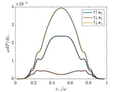
Figure 1: Here we plot the case of $\xi=1$, $\kappa=1$ and $N=5$ for the laser pulse described in the text. The fully colored lines is the result using the semiclassical approach, while the black dots on top is the same result using the Volkov state. The arrows denote the spin state of the produced electron and positron respectively, with the up-arrow denoting spin along the quantization axis $(z)$. The label $\boldsymbol{e}_{\parallel}$ and $\boldsymbol{e}_{\perp}$ denotes, respectively, that the incoming photon has polarization parallel or perpendicular to the polarization of the laser pulse. The remaining 5 possible combinations of spins and polarization are not plotted, as they coincide with the already plotted curves, however in all cases, there is agreement.

IV Discussion

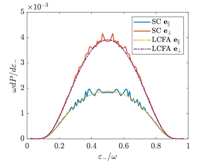
Figure 2: Here we plot the case of $\xi=5$, $\kappa=1$ and $N=5$ which has been summed over the spins, but showing the dependence of the probability depending on the relative photon polarizations. We compare the full result with that of the LCFA.

We have now shown how one may calculate the pair production probabilities using the semiclassical approach, and the approach using the Volkov state. We will compare the two approaches using an example of a linearly polarized laser pulse given by $a_{1}^{\mu}=\{0,a_{x},0,0\}$ and $a_{2}^{\mu}=\{0,0,a_{y},0\}$, $k^{\mu}_{0}=\{\omega_{0},0,0,-\omega_{0}\}$ and $k$ is in the opposite direction of $k_{0}$ and the spin quantization axis is along the momentum of $k$. We then choose as a model of our pulse

$$f_{1}(\varphi)=d(\varphi)\text{cos}(\varphi),$$ (30)

$$f_{2}(\varphi)=0,$$ (31)

$$d(\varphi) =\begin{cases}\text{sin}^{4}\left(\frac{\varphi}{2N}\right),&0<\varphi<2\pi N\\ 0.&\text{otherwise}\end{cases}$$ (32)

We define the invariant quantities $\xi$ and $\kappa$ in terms of their peak value which leads to the values

$$\xi=\frac{ea_{x}}{m},$$ (33)

$$\kappa=\frac{e\sqrt{\left|(F^{\mu\nu}k_{\nu})^{2}\right|}}{m^{3}}=\frac{2\omega\omega_{0}ea_{x}}{m^{3}}$$ (34)

where $F^{\mu\nu}$ is the peak value of the electromagnetic field tensor of the laser pulse. The parameter $\xi$ controls if the process involves single photons from the external field $(\xi\ll 1)$ or many photons, $(\xi\gg 1)$. The $\kappa$ parameter measures the field experienced by one of the produced particles (if all the energy went to this particle), relative to the Schwinger critical field, in its rest frame. When $\kappa$ is small, the pair production process is heavily suppressed by an exponential “tunneling” factor $e^{-8/3\kappa}$, within the local constant field approximation (LCFA), see e.g. Ritus (1985). It is proposed, in the context of the LUXE experiment, to see this behavior Hartin et al. (2019); Abramowicz et al. (2019). It is kept in mind that the experimental setup would involve a target to produce gamma rays from an electron beam via Bremsstrahlung, which would then collide with the laser pulse. We consider the case where the gamma ray photon has the same energy as the initial electron, which is reasonable as the largest contribution comes from these photons due to the mentioned tunneling suppression factor. In both of the planned experiments at SLAC and DESY the pulse duration of around $30$ fs at full width half maximum of the intensity corresponds to roughly $N=43$ for our choice of the pulse shape, and therefore we will use this for those cases along with $\omega_{0}=1.55$ eV. In Fig. (1) we show an example of $\xi=1$, $\kappa=1$ and $N=5$ where we have plotted the result from the semiclassical approach along with that from the Volkov state, and see that the results are indistinguishable. We have also checked for other values of these parameters, and also for the situtation where the laser beam is not counterpropagating with the incoming photon, and in every case there is as good agreement as seen in Fig. (1). It has also been checked that the mentioned additional integral which arises for pair production, but not in radiation emission, plays a role for the result, and therefore that it has been handled correctly. In the LUXE experiment it is planned that the first stage of the experiment is done at $\xi=2$ using a 30 TW laser Ritus (1985). In the SLAC experiment, a 17 TW laser is available which it is envisaged to focus down to the diffraction limit yielding $\xi=7.3$. The difference here is therefore that the first stage of the LUXE experiment is set more conservatively in terms of focusing the laser pulse. Both experiments plan on achieving $\xi>5$ and therefore in Fig. (2) we verify that when $\xi=5$ and $\kappa=1$, one may to good accuracy use the LCFA, which means using the formula for pair production in a constant crossed field, which can be found in e.g. Baier et al. (1998), at each instant of the laser pulse. However for the case of a potential first stage of these experiments,

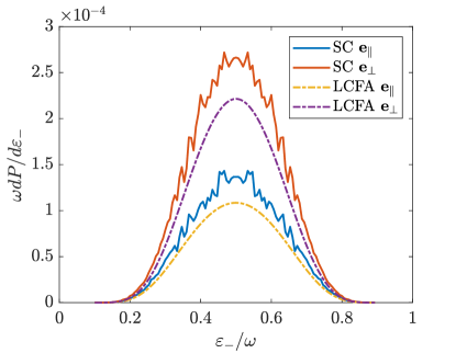
Figure 3: Here we show the case of $\xi=2$, $\kappa=0.4$ and $N=43$ which arises for a photon energy of $17.5$ GeV. This result therefore applies to the first stage of the proposed LUXE experiment Abramowicz et al. (2019).

where the fully focused pulse may not yet be achieved, we will see deviations from the LCFA result as $\xi$ goes closer to $1$. As pointed out by Ritus in Ritus (1985) in section 13, for the case of a monochromatic wave, if $\xi$ is not large, or if $\kappa\ll\xi/\sqrt{1+\xi^{2}}$ deviations from the LCFA arise. Most importantly, the overall pair production rate starts to deviate from the LCFA result. This can be seen in Fig. (3) and (4). In general, the pair production probability is larger than predicted by the LCFA when $\xi$ approaches $1$ from above. For the case shown in Fig. (4) the polarization averaged total probability in the exact case is 27% larger than that using the LCFA and for the case in Fig. (3) it is 23%. An interesting prediction seen in Ritus (1985) is that the pair production probability depends on the relative polarization between the laser pulse and the incoming photon. In particular it is shown that for the monochromatic wave and for $\kappa\ll 1$ the pair production rate for different relative polarizations obey $W_{\perp}=2W_{\parallel}$ and $W_{\perp}=3/2W_{\parallel}$ when $\kappa\gg 1$. This prediction has not been experimentally verified. As shown in Baier et al. (1998) the strong field can be seen as a dispersive medium, where the pair production corresponds to the imaginary part of the refractive index of this medium, the real part of which can be obtained by the Kramers-Kronig relations, i.e. the process of vacuum birefringence in QED. This process has been extensively studied Heinzl et al. (2006); Di Piazza et al. (2006); Adler (2007); Karbstein et al. (2015); Bregant et al. (2008); Bakalov et al. (1994); King and Elkina (2016); Wistisen and Uggerhøj (2013); Bragin et al. (2017); Denisov et al. (2017); Karbstein (2018); Briscese (2018), but not yet experimentally observed. Therefore the clear demonstration of the pair production rate’s dependence on the relative polarization is an indirect detection of the vacuum birefringence of QED. For the cases shown in Fig. (3) and (4) we have that $W_{\perp}=2.05W_{\parallel}$ and $W_{\perp}=2.04W_{\parallel}$, respectively. However for this measurement one would need polarized gamma rays, which can be obtained using either Compton back scattering on a small fraction of the laser pulse, or produced using a crystal target and the process of coherent bremsstrahlung, see e.g. Ter-Mikaelian (1972). A calculation of this is, however, beyond the scope of the current paper.

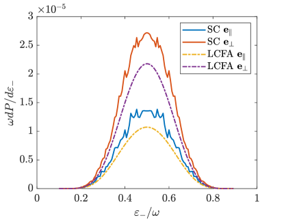
Figure 4: Here we show the case of $\xi=2$, $\kappa=0.3$ and $N=43$ which arises for a photon energy of $13.0$ GeV, which could be observed in a potential first stage of the SLAC E320 experiment, before the strongest focusing is achieved.

V Conclusion

We have shown how the semiclassical approach of Baier, Katkov and Strakhovenko may be recast in a form suitable for numerical implementation, allowing one to calculate the pair production probability in an arbitrary external field and for any photon polarization and electron-positron spins. We compared the results for a case where an exact solution is known, namely the Volkov state describing an electron-positron in a laser wave. In this case the results are indistinguishable. We investigated the size of the deviations from the local constant field approximation for experiments planned in the near future, when $\xi$ is not large. We saw that when $\xi=2$ deviations of around 25% in the overall rate should be expected. Finally the presented numerical approach allows to study polarization effects in pair production even in complicated fields and we used this to see that the probability of pair production in the two states of polarization, parallel and orthogonal to the linearly polarized laser pulse, still yields a factor of roughly $2$, even though $\kappa$ is not negligible and that we are dealing with a laser pulse rather than a monochromatic wave.

VI Acknowledgements

The author would like to thank Antonino Di Piazza for reading the manuscript and providing useful comments. T. N. Wistisen was supported by the Alexander von Humboldt-Stiftung for this work.

References

- Bula et al. (1996) C. Bula, K.T. McDonald, E.J. Prebys, C. Bamber, S. Boege, T. Kotseroglou, A.C. Melissinos, D.D. Meyerhofer, W. Ragg, D.L. Burke, et al., “Observation of nonlinear effects in Compton scattering,” Phys. Rev. Lett. 76, 3116 (1996).
- Bak et al. (1985) J. Bak, J.A. Ellison, B. Marsh, F.E. Meyer, O. Pedersen, J.B.B. Petersen, E. Uggerhøj, K. Østergaard, S.P. Møller, A.H. Sørensen, and M. Suffert, “Channeling radiation from 2-55 GeV/c electrons and positrons: (I). Planar case,” Nucl. Phys. B. 254, 491 – 527 (1985).
- Bak et al. (1988) J.F. Bak, J.A. Ellison, B. Marsh, F.E. Meyer, O. Pedersen, J.B.B. Petersen, E. Uggerhøj, S.P. Møller, H. Sørensen, and M. Suffert, “Channeling radiation from 2 to 20 GeV/c electrons and positrons (II).: Axial case,” Nucl. Phys. B. 302, 525 – 558 (1988).
- Swent et al. (1979) R. L. Swent, R. H. Pantell, M. J. Alguard, B. L. Berman, S. D. Bloom, and S. Datz, “Observation of channeling radiation from relativistic electrons,” Phys. Rev. Lett. 43, 1723–1726 (1979).
- Andersen et al. (1981) J.U. Andersen, K.R. Eriksen, and E. Laegsgaard, “Planar-Channeling Radiation and Coherent Bremsstrahlung for MeV Electrons,” Phys. Scr. 24, 588 (1981).
- Andersen et al. (1982) J.U. Andersen, E. Bonderup, E. Laegsgaard, B.B. Marsh, and A.H. Sørensen, “Axial channeling radiation from MeV electrons,” Nucl. Instrum. Methods Phys. Res. 194, 209 – 224 (1982).
- Klein et al. (1985) R. K. Klein, J. O. Kephart, R. H. Pantell, H. Park, B. L. Berman, R. L. Swent, S. Datz, and R. W. Fearick, “Electron channeling radiation from diamond,” Phys. Rev. B 31, 68–92 (1985).
- Alguard et al. (1979) M. J. Alguard, R. L. Swent, R. H. Pantell, B. L. Berman, S. D. Bloom, and S. Datz, “Observation of radiation from channeled positrons,” Phys. Rev. Lett. 42, 1148–1151 (1979).
- Andersen et al. (2012) K. K. Andersen, J. Esberg, H. Knudsen, H. D. Thomsen, U. I. Uggerhøj, P. Sona, A. Mangiarotti, T. J. Ketel, A. Dizdar, and S. Ballestrero (CERN NA63), “Experimental investigations of synchrotron radiation at the onset of the quantum regime,” Phys. Rev. D 86, 072001 (2012).
- Uggerhøj (2005) U. I. Uggerhøj, “The interaction of relativistic particles with strong crystalline fields,” Rev. Mod. Phys. 77, 1131–1171 (2005).
- Wistisen et al. (2014) T. N. Wistisen, K. K. Andersen, S. Yilmaz, R. Mikkelsen, J. L. Hansen, U. I. Uggerhøj, W. Lauth, and H. Backe, “Experimental realization of a new type of crystalline undulator,” Phys. Rev. Lett. 112, 254801 (2014).
- Di Piazza et al. (2010) A. Di Piazza, K. Z. Hatsagortsyan, and C. H. Keitel, “Quantum Radiation Reaction Effects in Multiphoton Compton Scattering,” Phys. Rev. Lett. 105, 220403 (2010).
- Neitz and Di Piazza (2013) N. Neitz and A. Di Piazza, “Stochasticity effects in quantum radiation reaction,” Phys. Rev. Lett. 111, 054802 (2013).
- Blackburn et al. (2014) T. G. Blackburn, C. P. Ridgers, J. G. Kirk, and A. R. Bell, “Quantum radiation reaction in laser–electron-beam collisions,” Phys. Rev. Lett. 112, 015001 (2014).
- Ji et al. (2014) L. L. Ji, A. Pukhov, I. Yu. Kostyukov, B. F. Shen, and K. Akli, “Radiation-reaction trapping of electrons in extreme laser fields,” Phys. Rev. Lett. 112, 145003 (2014).
- Ilderton and Torgrimsson (2013) A. Ilderton and G. Torgrimsson, “Radiation reaction in strong field QED,” Physics Letters B 725, 481 – 486 (2013).
- Dinu et al. (2016) V. Dinu, C. Harvey, A. Ilderton, M. Marklund, and G. Torgrimsson, “Quantum radiation reaction: From interference to incoherence,” Phys. Rev. Lett. 116, 044801 (2016).
- Vranic et al. (2014) M. Vranic, J. L. Martins, J. Vieira, R. A. Fonseca, and L. O. Silva, “All-optical radiation reaction at ,” Phys. Rev. Lett. 113, 134801 (2014).
- Seipt and Kämpfer (2012) D. Seipt and B. Kämpfer, “Two-photon Compton process in pulsed intense laser fields,” Phys. Rev. D 85, 101701 (2012).
- Mackenroth and Di Piazza (2013) F. Mackenroth and A. Di Piazza, “Nonlinear Double Compton Scattering in the Ultrarelativistic Quantum Regime,” Phys. Rev. Lett. 110, 070402 (2013).
- Dinu and Torgrimsson (2019a) V. Dinu and G. Torgrimsson, “Single and double nonlinear Compton scattering,” Phys. Rev. D 99, 096018 (2019a).
- King (2015) B. King, “Double Compton scattering in a constant crossed field,” Phys. Rev. A 91, 033415 (2015).
- Dinu and Torgrimsson (2019b) V. Dinu and G. Torgrimsson, “Approximating higher-order nonlinear QED processes with first-order building blocks,” (2019b), arXiv:1912.11015 [hep-ph] .
- Wistisen et al. (2018) T. N. Wistisen, A. Di Piazza, H. V. Knudsen, and U. I. Uggerhøj, “Experimental evidence of quantum radiation reaction in aligned crystals,” Nat. Commun. 9, 795 (2018).
- Cole et al. (2018) J. M. Cole, K. T. Behm, E. Gerstmayr, T. G. Blackburn, J. C. Wood, C. D. Baird, M. J. Duff, C. Harvey, A. Ilderton, A. S. Joglekar, K. Krushelnick, S. Kuschel, M. Marklund, P. McKenna, C. D. Murphy, K. Poder, C. P. Ridgers, G. M. Samarin, G. Sarri, D. R. Symes, A. G. R. Thomas, J. Warwick, M. Zepf, Z. Najmudin, and S. P. D. Mangles, “Experimental evidence of radiation reaction in the collision of a high-intensity laser pulse with a laser-wakefield accelerated electron beam,” Phys. Rev. X 8, 011020 (2018).
- Poder et al. (2018) K. Poder, M. Tamburini, G. Sarri, A. Di Piazza, S. Kuschel, C. D. Baird, K. Behm, S. Bohlen, J. M. Cole, D. J. Corvan, M. Duff, E. Gerstmayr, C. H. Keitel, K. Krushelnick, S. P. D. Mangles, P. McKenna, C. D. Murphy, Z. Najmudin, C. P. Ridgers, G. M. Samarin, D. R. Symes, A. G. R. Thomas, J. Warwick, and M. Zepf, “Experimental signatures of the quantum nature of radiation reaction in the field of an ultraintense laser,” Phys. Rev. X 8, 031004 (2018).
- Wistisen et al. (2019) T. N. Wistisen, A. Di Piazza, C. F. Nielsen, A. H. Sørensen, and U. I. Uggerhøj (CERN NA63), “Quantum radiation reaction in aligned crystals beyond the local constant field approximation,” Phys. Rev. Research 1, 033014 (2019).
- Abramowicz et al. (2019) H. Abramowicz et al., “Letter of Intent for the LUXE Experiment,” (2019), arXiv:1909.00860 [physics.ins-det] .
- Meuren (2019) S. Meuren, “Probing Strong-field QED at FACET-II (SLAC E-320),” (2019).
- Turcu et al. (2016) I. C. E. Turcu et al., “High field physics and QED experiments at ELI-NP,” Rom. Rep. Phys. 68, S145 (2016).
- Breit and Wheeler (1934) G. Breit and John A. Wheeler, “Collision of two light quanta,” Phys. Rev. 46, 1087–1091 (1934).
- Krajewska and Kamiński (2012) K. Krajewska and J. Z. Kamiński, “Breit-Wheeler process in intense short laser pulses,” Phys. Rev. A 86, 052104 (2012).
- Titov et al. (2013) A. I. Titov, B. Kämpfer, H. Takabe, and A. Hosaka, “Breit-Wheeler process in very short electromagnetic pulses,” Phys. Rev. A 87, 042106 (2013).
- Di Piazza (2016) A. Di Piazza, “Nonlinear Breit-Wheeler Pair Production in a Tightly Focused Laser Beam,” Phys. Rev. Lett. 117, 213201 (2016).
- Heinzl et al. (2010) T. Heinzl, A. Ilderton, and M. Marklund, “Finite size effects in stimulated laser pair production,” Phys. Lett. B 692, 250 – 256 (2010).
- Titov et al. (2012) A. I. Titov, H. Takabe, B. Kämpfer, and A. Hosaka, “Enhanced subthreshold production in short laser pulses,” Phys. Rev. Lett. 108, 240406 (2012).
- Jansen and Müller (2016) M. J. A. Jansen and C. Müller, “Strong-field Breit-Wheeler pair production in short laser pulses: Identifying multiphoton interference and carrier-envelope-phase effects,” Phys. Rev. D 93, 053011 (2016).
- Nousch et al. (2016) T. Nousch, D. Seipt, B. Kämpfer, and A. I. Titov, “Spectral caustics in laser assisted Breit-Wheeler process,” Physics Letters B 755, 162 – 167 (2016).
- Jansen et al. (2016) M. J. A. Jansen, J. Z. Kamiński, K. Krajewska, and C. Müller, “Strong-field Breit-Wheeler pair production in short laser pulses: Relevance of spin effects,” Phys. Rev. D 94, 013010 (2016).
- Meuren et al. (2015a) S. Meuren, K. Z. Hatsagortsyan, C. H. Keitel, and A. Di Piazza, “Polarization-operator approach to pair creation in short laser pulses,” Phys. Rev. D 91, 013009 (2015a).
- Meuren et al. (2016) S. Meuren, C. H. Keitel, and A. Di Piazza, “Semiclassical picture for electron-positron photoproduction in strong laser fields,” Phys. Rev. D 93, 085028 (2016).
- Meuren et al. (2015b) S. Meuren, K. Z. Hatsagortsyan, C. H. Keitel, and A. Di Piazza, “High-energy recollision processes of laser-generated electron-positron pairs,” Phys. Rev. Lett. 114, 143201 (2015b).
- Baier and Katkov (1968) V.N. Baier and V.M. Katkov, “Processes involved in the motion of high energy particles in a magnetic field,” J. Exp. Theor. Phys. 26, 854 (1968).
- Baier et al. (1998) V.N. Baier, V.M. Katkov, and V.M. Strakhovenko, Electromagnetic Processes at High Energies in Oriented Single Crystals (World Scientific, 1998).
- Wöllert et al. (2015) A. Wöllert, H. Bauke, and C. H. Keitel, “Spin polarized electron-positron pair production via elliptical polarized laser fields,” Phys. Rev. D 91, 125026 (2015).
- Chen et al. (2019) Y.-Y. Chen, P.-L. He, R. Shaisultanov, K. Z. Hatsagortsyan, and C. H. Keitel, “Polarized positron beams via intense two-color laser pulses,” Phys. Rev. Lett. 123, 174801 (2019).
- Wan et al. (2020) F. Wan, R. Shaisultanov, Y.-F. Li, K. Z. Hatsagortsyan, C. H. Keitel, and J.-X. Li, “Ultrarelativistic polarized positron jets via collision of electron and ultraintense laser beams,” Physics Letters B 800, 135120 (2020).
- Wistisen and Di Piazza (2019a) T. N. Wistisen and A. Di Piazza, “Complete treatment of single-photon emission in planar channeling,” Phys. Rev. D 99, 116010 (2019a).
- Wistisen and Di Piazza (2018) T. N. Wistisen and A. Di Piazza, “Impact of the quantized transverse motion on radiation emission in a Dirac harmonic oscillator,” Phys. Rev. A 98, 022131 (2018).
- Wistisen and Di Piazza (2019b) T. N. Wistisen and A. Di Piazza, “Numerical approach to the semiclassical method of radiation emission for arbitrary electron spin and photon polarization,” Phys. Rev. D 100, 116001 (2019b).
- Wistisen (2014) T. N. Wistisen, “Interference effect in nonlinear Compton scattering,” Phys. Rev. D 90, 125008 (2014).
- Wistisen (2015) T. N. Wistisen, “Quantum synchrotron radiation in the case of a field with finite extension,” Phys. Rev. D 92, 045045 (2015).
- Ritus (1985) V.I. Ritus, “Quantum effects of the interaction of elementary particles with an intense electromagnetic field,” Journal of Soviet Laser Research 6, 497–617 (1985).
- Hartin et al. (2019) A. Hartin, A. Ringwald, and N. Tapia, “Measuring the boiling point of the vacuum of quantum electrodynamics,” Phys. Rev. D 99, 036008 (2019).
- Heinzl et al. (2006) T. Heinzl, B. Liesfeld, K.U. Amthor, H. Schwoerer, R. Sauerbrey, and A. Wipf, “On the observation of vacuum birefringence,” Optics Communications 267, 318 – 321 (2006).
- Di Piazza et al. (2006) A. Di Piazza, K. Z. Hatsagortsyan, and C. H. Keitel, “Light diffraction by a strong standing electromagnetic wave,” Phys. Rev. Lett. 97, 083603 (2006).
- Adler (2007) S. L. Adler, “Vacuum birefringence in a rotating magnetic field,” Journal of Physics A: Mathematical and Theoretical 40, F143 (2007).
- Karbstein et al. (2015) F. Karbstein, H. Gies, M. Reuter, and M. Zepf, “Vacuum birefringence in strong inhomogeneous electromagnetic fields,” Phys. Rev. D 92, 071301 (2015).
- Bregant et al. (2008) M. Bregant, G. Cantatore, S. Carusotto, R. Cimino, F. Della Valle, G. Di Domenico, U. Gastaldi, M. Karuza, V. Lozza, E. Milotti, E. Polacco, G. Raiteri, G. Ruoso, E. Zavattini, and G. Zavattini (PVLAS Collaboration), “Limits on low energy photon-photon scattering from an experiment on magnetic vacuum birefringence,” Phys. Rev. D 78, 032006 (2008).
- Bakalov et al. (1994) D. Bakalov, G. Cantatore, G. Carugno, S. Carusotto, P. Favaron, F. Della Valle, I. Gabrielli, U. Gastaldi, E. Iacopini, P. Micossi, E. Milotti, R. Onofrio, R. Pengo, F. Perrone, G. Petrucci, E. Polacco, C. Rizzo, G. Ruoso, E. Zavattini, and G. Zavattini, “PVLAS: Vacuum Birefringence and production and detection of nearly massless, weakly coupled particles by optical techniques.” Nuclear Physics B - Proceedings Supplements 35, 180 – 182 (1994).
- King and Elkina (2016) B. King and N. Elkina, “Vacuum birefringence in high-energy laser-electron collisions,” Phys. Rev. A 94, 062102 (2016).
- Wistisen and Uggerhøj (2013) T. N. Wistisen and U. I. Uggerhøj, “Vacuum birefringence by Compton backscattering through a strong field,” Phys. Rev. D 88, 053009 (2013).
- Bragin et al. (2017) S. Bragin, S. Meuren, C. H. Keitel, and A. Di Piazza, “High-energy vacuum birefringence and dichroism in an ultrastrong laser field,” Phys. Rev. Lett. 119, 250403 (2017).
- Denisov et al. (2017) V.I. Denisov, E.E. Dolgaya, and V.A. Sokolov, “Nonperturbative QED vacuum birefringence,” Journal of High Energy Physics 2017, 105 (2017).
- Karbstein (2018) F. Karbstein, “Vacuum birefringence in the head-on collision of x-ray free-electron laser and optical high-intensity laser pulses,” Phys. Rev. D 98, 056010 (2018).
- Briscese (2018) F. Briscese, “Collective behavior of light in vacuum,” Phys. Rev. A 97, 033803 (2018).
- Ter-Mikaelian (1972) M. L. Ter-Mikaelian, High-energy electromagnetic processes in condensed media (Wiley-Interscience, 1972).