Ancestral lines under recombination

Solving the recombination equation has been a long-standing challenge of deterministic population genetics. We review recent progress obtained by introducing ancestral processes, as traditionally used in the context of stochastic models of population genetics, into the deterministic setting. With the help of an ancestral partitioning process, which is obtained by letting population size tend to infinity (without rescaling parameters or time) in an ancestral recombination graph, we obtain the solution to the recombination equation in a transparent form.

1. Introduction

Recombination is a genetic mechanism that ‘mixes’ or ‘reshuffles’ the genetic material of different individuals from generation to generation; it takes place in the course of sexual reproduction. Models that describe the evolution of populations under recombination (in isolation or in combination with other processes) are among the major challenges in population genetics. Besides being of theoretical and mathematical interest, they play a major role in inference from population sequence data; compare the contribution of Dutheil [21] in this volume.

In line with the general situation in population genetics, models of recombination come in two categories, deterministic and stochastic. In addition, there are versions in discrete and in continuous time, both of which will be considered below. In particular, our approach will result in a unified treatment of both.

Deterministic approaches assume that the population is so large that a law of large numbers applies and random fluctuations may be neglected. The resulting models are (systems of) ordinary differential equations or (discrete-time) dynamical systems, which describe the evolution of the genetic composition of a population under recombination in the usual forward direction of time; for review, see [32, 17, 16]. The genetic composition is described via a probability distribution (or measure) on a space of sequences of finite length. The equations are nonlinear and notoriously difficult to solve. Elucidating the underlying structure and finding solutions was a challenge to theoretical population geneticists for nearly a century. Indeed, the first studies go back to Jennings [31] in 1917 and Robbins [35] in 1918. Geiringer [26] in 1944 and Bennett [13] in 1954 were the first to state the generic general form of the solution in terms of a convex combination of certain basis functions, and evaluated the corresponding coefficients recursively for sequences with a small number of sites. The approach was later continued within the systematic framework of genetic algebras; compare [32, 29]. The recursions for the coefficients were worked out in fairly general form by Dawson [19]. In any case, however, the work is technically cumbersome and yields limited insight into the underlying mathematical structure.

Stochastic approaches, on the other hand, take into account the fluctuations due to finite population size. The evolution of the composition of a population over time is described via a Moran or a Wright–Fisher model with recombination. The first study goes back to Ohta and Kimura [34] in 1969. Over the decades, two major lines of research have emerged. There has been continuous interest in how the correlations between sites (known as linkage disequilibria) will develop; see [34, 36] and the overviews in [30, Ch. 5.4], [20, Ch. 3.3 and 8.2] or [37, Ch. 7.2.4]. The explicit time course of the genetic composition of the population is even more challenging, due to an intricate interplay of resampling and recombination; compare  [34, 36, 7, 15] as well as [20, Ch. 8.2]. These questions are usually approached forward in time.

The second line of research is concerned with genealogical aspects. Here, one starts with a sample taken from the present population and traces back the ancestry of the various sequence segments the individuals are composed of. The standard tool for this purpose is the ancestral recombination graph (ARG), first formulated by Hudson [28] in 1983. His original version was for two sites, but generalisations to an arbitrary number of sites [27, 14] and continuous versions [20, Ch. 3.4] are immediate.

The stochastic models of recombination are related to their deterministic counterparts via a dynamical law of large numbers as population size tends to infinity. Nevertheless, deterministic and stochastic approaches have largely led separate lives for decades. It is the goal of this article to review recent progress to build bridges between them by introducing the genealogical picture into the deterministic equations. The corresponding ancestral processes remain random even in the deterministic limit, since they describe the history of single individuals (or a finite sample thereof). They lead to stochastic representations of the solutions of the deterministic equations and shed new light both on their dynamics and their asymptotic behaviour. A similar programme has been carried out for mutation-selection models; see [4, 18] as well as the review [8].

2. Moran model with recombination

Let us start from the Moran model with recombination (in continuous time), which we recapitulate here from [15, 23, 24]. We consider a linear arrangement (or sequence) of $n$ discrete positions called sites, which are collected in the set $S=\{1,\dotsc,n\}$. A site may be understood as a nucleotide site or a gene locus. We will throughout consider sequences as (haploid) individuals, that is, we think at the level of gametes (rather than that of diploid individuals that carry two copies of the genetic information). Site $i$ is occupied by a letter $x_{i}\in X_{i}$, where $X_{i}$ is a finite set, $1\leqslant i\leqslant n$. If sites are nucleotide sites, a natural choice for each $X_{i}$ is the nucleotide alphabet $\{\rm{A,G,C,T}\}$; if sites are gene loci, $X_{i}$ is the set of alleles that can occur at locus $i$. The genetic type of each individual is thus described by the sequence $x=(x_{1},x_{2},\dotsc,x_{n})\in X_{1}\times\dots\times X_{n}=\mathrel{\mathop{:}}X$, where $X$ is the type space.

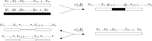
Figure 2.1. Result of a double crossover between sites $i$ and $i+1$ and between $j$ and $j+1$ ($1\leqslant i<j<n$). Top: full details of parental sequences; bottom: a version that marginalises over the letters that do not end up in the offspring.

In this setting, recombination means that a new individual is formed as a ‘mixture’ of an (ordered) pair of parents, say $x$ and $y$. We describe this mixture with the help of a partition $\mathcal{A}$ of $S$ into two parts. Namely, $\mathcal{A}=\{A_{1},A_{2}\}$ means that the new individual copies the letters at all sites in $A_{1}$ from the first individual and the letters at all sites in $A_{2}$ from the second; this happens via a number of crossovers between the sequences, as illustrated in Figure 2.1. For reasons of symmetry, we need not keep track of which part (or block) was ‘maternal’ and which was ‘paternal’. Altogether, whenever an offspring is created, its sites are partitioned between parents according to $\mathcal{A}$ with probability $r(\mathcal{A})$, where $r(\mathcal{A})\geqslant 0$, $\sum_{\mathcal{A}\in\mathcal{P}_{2}(S)}r(\mathcal{A})\leqslant 1$, and $\mathcal{P}_{2}(S)$ is the set of all partitions of $S$ into two parts. The sum $\sum_{\mathcal{A}\in\mathcal{P}_{2}(S)}r(\mathcal{A})$ is the probability that some recombination event takes place during reproduction. With probability $r(\boldsymbol{1})=1-\sum_{\!\mathcal{A}\in\mathcal{P}_{2}(S)}r(\mathcal{A})$, there is no recombination, in which case the offspring is the full copy of a single parent; here $\boldsymbol{1}\mathrel{\mathop{:}}=\{S\}$, the coarsest partition. We write $\mathcal{P}_{\!\leqslant 2}(S)\mathrel{\mathop{:}}=\mathcal{P}_{2}(S)\cup\{\boldsymbol{1}\}$ for the set of partitions into at most two parts, and $\mathcal{P}(S)$ for the set of all partitions of $S$. The collection $\{r(\mathcal{A})\}_{\mathcal{A}\in\mathcal{P}_{\leqslant 2}(S)}$ is known as the recombination distribution [16, p. 55].

Consider now a population of a constant number $N$ of haploid individuals (that is, gametes) that evolves in continuous time as described next (see Figure 2.2). Each individual dies at rate $\mu$, that is, it has an exponential lifespan with parameter $\mu$ (this parameter simply sets the time scale). When an individual dies, it is replaced by a new one as follows. First, draw a partition $\mathcal{A}$ according to the recombination distribution. Then, draw $|\mathcal{A}|$ parents from the population (the parents may include the individual that is about to die), uniformly and with replacement, where $|\mathcal{A}|$ is the number of parts in $\mathcal{A}$. If $|\mathcal{A}|=2$, $\mathcal{A}$ is of the form $\{A_{1},A_{2}\}$, and the offspring inherits the sites in $A_{1}$ from the first parent and the sites in $A_{2}$ from the second, as described above. If $|\mathcal{A}|=1$ (and thus $\mathcal{A}=\boldsymbol{1}$), the offspring is a full copy of a single parent (again chosen uniformly from among all individuals); this is called a (pure) resampling event. All events are independent of each other. Note that the model may equivalently be formulated in terms of reproducing rather than dying individuals, in the following way. Every individual reproduces at rate $\mu$, draws a partition $\mathcal{A}$ according to the recombination distribution, and picks $|\mathcal{A}|-1$ partners from the population; the offspring individual is pieced together according to $\mathcal{A}$ from the ‘active’ individual and the partners, and replaces a uniformly chosen individual.

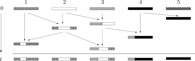
Figure 2.2. A realisation of the Moran model with recombination forward in time, with $N=5$. For example, in the second event, individual 3 is replaced by a recombined copy of individuals 2 and 3.

We identify the population at time $t$ with a (random) counting measure $Z^{(N)}_{t}$ on $X$, where the upper index indicates the dependence on populaton size. Namely, $Z^{(N)}_{t}(\{x\})\geqslant 0$ denotes the number of individuals of type $x\in X$ at time $t$, and $Z^{(N)}_{t}(\mathbb{A})=\sum_{x\in\mathbb{A}}Z^{(N)}_{t}(\{x\})$ for $\mathbb{A}\subseteq X$. We can also write

$$Z^{(N)}_{t}=\sum_{x\in X}Z^{(N)}_{t}(\{x\})\,\delta_{x}$$

in terms of point measures on $x$. Since our Moran population has constant size $N$, we have $\|Z^{(N)}_{t}\|=N$ for all times, where $\|Z^{(N)}_{t}\|\mathrel{\mathop{:}}=Z^{(N)}_{t}(X)=\sum_{x\in X}Z^{(N)}_{t}(\{x\})$ is the norm (or total variation) of $Z^{(N)}_{t}$.

This way, $(Z^{(N)}_{t})_{t\geqslant 0}$ is a Markov chain in continuous time with values in

(2.1) $$E\mathrel{\mathop{:}}=\big{\{}z\in\{0,\dotsc,N\}^{\lvert X\rvert}:\|z\|=N\big{\}},$$

where $\lvert X\rvert$ is the number of elements in $X$. We will describe the action of recombination on (positive) measures with the help of so-called recombinators as introduced in [2]. Let $\boldsymbol{M}_{+}(X)$ be the set of all positive, finite measures on $X$, where we understand $\boldsymbol{M}_{+}(X)$ to include the zero measure. Define the canonical projection $\pi_{I}\colon X\mapsto\mbox{\LARGE$\times$}_{i\in I}X_{i}=\mathrel{\mathop{:}}X_{I}$, for $\varnothing\neq I\subseteq S=\{1,\ldots,n\}$, by $\pi_{I}(x)=(x_{i})_{i\in I}=\mathrel{\mathop{:}}x_{I}$ as usual. For $\omega\in\boldsymbol{M}_{+}(X)$, the shorthand $\omega^{I}\mathrel{\mathop{:}}=\pi_{I}.\hskip 0.5pt\omega=\omega\circ\pi_{I}^{-1}$ indicates the marginal measure with respect to the sites in $I$, where $\pi_{I}^{-1}$ is the preimage of $\pi_{I}$, and the operation . (where the dot is on the line and should not be confused with a multiplication sign) denotes the pushforward of $\omega$ w.r.t. $\pi_{I}$. In terms of coordinates, the definition may be spelled out as

$$\omega^{I}(x_{I})=(\omega\circ\pi_{I}^{-1})(x_{I})=\omega\big{(}\{x\in X:\pi_{I}(x)=x_{I}\}\big{)},\quad x_{I}\in X_{I}.$$

Note that $\omega^{S}=\omega$.

Consider now $\mathcal{A}=\{A_{1},\ldots,A_{m}\}\in\mathcal{P}(S)$ and $\omega\in\boldsymbol{M}_{+}(X)$, and define the recombinator as

(2.2) $$R_{\mathcal{A}}(\omega)\mathrel{\mathop{:}}=\frac{1}{\|\omega\|^{m-1}}\,\bigotimes_{A\in\mathcal{A}}\omega^{A},$$

where $\otimes$ indicates the product measure and the definition extends consistently to $R_{\mathcal{A}}(0)=0$. Note that $R_{\boldsymbol{1}}(\omega)=\omega$. Clearly, $\|R_{\mathcal{A}}(\omega)\|=\|\omega\|$ for all $\omega\in\boldsymbol{M}_{+}(X)$. In particular, $R_{\mathcal{A}}$ turns $\omega\neq 0$ into the (normalised) product measure of its marginals with respect to the blocks in $\mathcal{A}$. If $Z_{t}=z$ is the current population, then $\frac{1}{\|z\|}R_{\mathcal{A}}(z)=\frac{1}{N}R_{\mathcal{A}}(z)$ is the type distribution that results when a hypothetical individual is created by drawing marginal types (as encoded by $\mathcal{A}\in\mathcal{P}(S)$) from the current population, uniformly and with replacement.

We now use the recombinators to reformulate the Moran model with recombination in a compact way. Namely, since all individuals die at rate $\mu$, the population loses type-$y$ individuals at rate $\mu Z^{(N)}_{t}(\{y\})$. Each loss is replaced by a new individual, which is sampled uniformly from $\frac{1}{N}R_{\mathcal{A}}(Z^{(N)}_{t})$ with probability $r(\mathcal{A})$ for $\mathcal{A}\in\mathcal{P}_{\!\leqslant 2}(S)$. Therefore, when $Z^{(N)}_{t}=z$, the transition to $z+\delta_{x}-\delta_{y}$ occurs at rate

(2.3) $$\lambda^{(N)}(z;\,y,\,x)\,=\!\sum_{\mathcal{A}\in\mathcal{P}_{\!\leqslant 2}(S)}\frac{1}{N}\varrho(\mathcal{A})\big{(}R_{\mathcal{A}}(z)\big{)}(\{x\})\,z(\{y\}),$$

where $\varrho(\mathcal{A})=\mu\,r(\mathcal{A})$ is a recombination rate (in line with the continuous-time model). The summand for $\mathcal{A}=\boldsymbol{1}$ corresponds to pure resampling, whereas all other summands include recombination. Note that $\lambda^{(N)}$ includes ‘silent transitions’ ($x=y$).

Law of large numbers. Consider now the family of processes $(Z_{t}^{(N)})_{t\geqslant 0}$ with $N\in\mathbb{N}$. Also, consider the normalised version $(\frac{1}{N}Z_{t}^{(N)})_{t\geqslant 0}$; note that $\frac{1}{N}Z_{t}^{(N)}$ is a random probability measure on $X$. For $N\to\infty$ and without any rescaling of the $\varrho(\mathcal{A})$ or of time, the sequence $(\frac{1}{N}Z_{t}^{(N)})_{t\geqslant 0}$ converges to the solution of the deterministic recombination equation

(2.4) $$\dot{\omega}_{t}\,=\!\!\!\!\sum_{\mathcal{A}\in\mathcal{P}_{\!2}(S)}\varrho(\mathcal{A})\big{(}R_{\mathcal{A}}(\omega_{t})-\omega_{t}\big{)}$$

with initial value $\omega_{0}\in\boldsymbol{P}(X)$ (the set of probability measures on $X$), where we assume that

$$\lim_{N\to\infty}\frac{Z_{0}^{(N)}}{N}\,=\,\omega_{0}.$$

The convergence to the differential equation (2.4) is a dynamical law of large numbers and due to [25, Thm. 11.2.1]. The precise statement as well as the proof are perfectly analogous to [7, Prop. 6], which assumes a slightly different recombination and sampling scheme, without consequence for the convergence claim.

3. Ancestral recombination graph and deterministic limit

Let us return to the finite-$N$ model and construct the type of an individual sampled randomly from the population at time $t$ (the ‘present’) by genealogical means. We do so by adapting the ARG (see [14] and, for overviews, [30, Ch. 5.4], [20, Ch. 3.3, 8.4] or [37, Ch. 7.2.4]) to our model and a sample of size 1.

The type of an individual at present, together with its ancestry, can thus be constructed by a three-step procedure as illustrated in Figure 3.1.

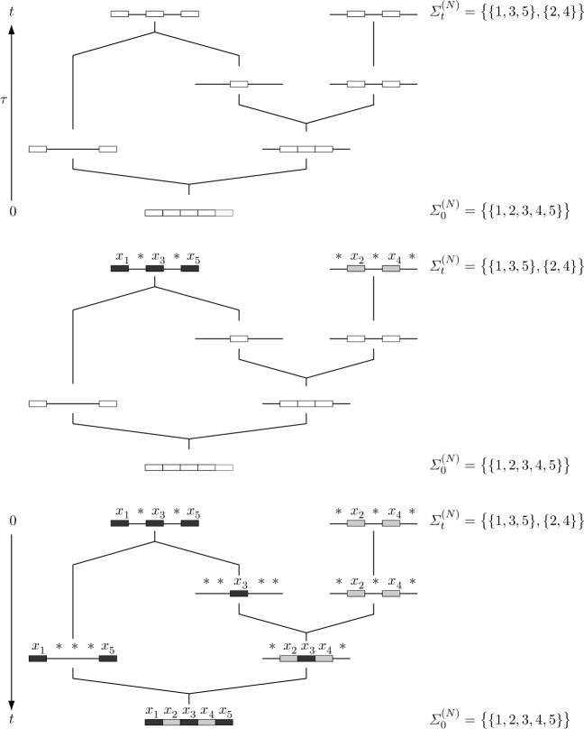
Figure 3.1. Example realisation of the partitioning process (top), assigning letters to the parts (middle), and propagating them downwards (bottom).

First, we run a partitioning process $(\varSigma^{(N)}_{\tau})_{0\leqslant\tau\leqslant t}$. Here, $(\varSigma^{(N)}_{\tau})_{\tau\geqslant 0}$ is a Markov chain in continuous time on $\mathcal{P}(S)$, whose time axis is directed into the past; we use the variables $t$ and $\tau$ throughout for forward and backward time, respectively, so $\tau=t$ in backward time corresponds to $t=0$ in forward time. The process starts with the coarsest partition $\varSigma^{(N)}_{0}=\boldsymbol{1}$, that is, we consider the (intact) sequence of one individual at time $t$. Then, $(\varSigma^{(N)}_{\tau})_{\tau\geqslant 0}$ describes the partitioning of sites into parental individuals at time $\tau$ before the present; sites in the same block (in different blocks) belong to the same (to different) individuals. Clearly, $\lvert\varSigma^{(N)}_{\tau}\rvert$ is the number of ancestral individuals at time $\tau$. The process $(\varSigma^{(N)}_{\tau})_{\tau\geqslant 0}$ consists of splitting and coalescence events (and combinations thereof), is independent of the types, and will be described in detail below.

In the second step, a letter is assigned to each site of $S$ at $\tau=t$ (that is, at forward time 0) as follows. For every part of $\varSigma^{(N)}_{t}$, pick an individual from the initial population $Z^{(N)}_{0}$ (without replacement) and copy its letters to the sites in the block considered. For illustration, also assign a colour to each block, thus indicating different parental individuals. In the last step, the letters and colours are propagated downwards (that is, forward in time) according to the realisation of $(\varSigma^{(N)}_{\tau})_{0\leqslant\tau\leqslant t}$ laid down in the first step.

Let us now describe the partitioning process more precisely, following [23, 24] but specialising to $\varSigma_{0}^{(N)}=\boldsymbol{1}$. Since we also trace back sites in subsets $U\subseteq S$ (rather than complete sequences), we need the corresponding marginal recombination rates

(3.1) $$\varrho^{U}\!(\mathcal{B})\,\mathrel{\mathop{:}}=\!\sum_{\begin{subarray}{c}\mathcal{A}\in\mathcal{P}_{\!\leqslant 2}(S)\\ \mathcal{A}|_{U}=\mathcal{B}\end{subarray}}\!\varrho(\mathcal{A})$$

for any $\mathcal{B}\in\mathcal{P}_{\!\leqslant 2}(U)$, where $\mathcal{A}|_{U}$ is the partition of $U$ induced by $\mathcal{A}$; namely, $\mathcal{A}|_{U}=\{A\cap U:A\in\mathcal{A},A\cap U\neq\varnothing\}$. Clearly, $\varrho^{S}(\mathcal{B})=\varrho(\mathcal{B})$ and $\varrho^{U}\!(\mathcal{B})$ is the sum of the rates of all recombination events that lead to partition $\mathcal{B}$ under the projection to $U$, as illustrated in Figure 3.2. Note that, for $|U|=1$, the only recombination parameter is $\varrho^{U}\!(\boldsymbol{1})=1$ (note that we use $\boldsymbol{1}$ to indicate the coarsest partition throughout, where the meaning is always clear from the upper index, so here $\boldsymbol{1}=\{U\}$).

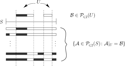
Figure 3.2. The marginal recombination rate for a partition $\mathcal{B}$ of a subset $U$ is the sum of all recombination rates for partitions $\mathcal{A}$ of the original set $S$ that lead to $\mathcal{B}$ under projection to $U$.

Suppose now that the current state is $\varSigma^{(N)}_{\tau}=\mathcal{A}=\{A_{1},\dotsc,A_{m}\}$ and denote by $\Delta$ the waiting time to the next event. The random variable $\Delta$ is exponentially distributed with parameter $m\mu$, since each block corresponds to an individual, and each individual is independently affected at rate $\mu$. When the event happens, choose one of the $m$ blocks, each with probability $\frac{1}{m}$. If $A_{j}$ is picked, $\varSigma^{(N)}_{\tau+\Delta}$ is obtained via a two-step procedure, namely a splitting step followed by a sampling step, namely:

1. In the splitting step, block $A_{j}$ turns into an intermediate state $\mathfrak{a}$ with probability $r^{A_{j}}(\mathfrak{a})$, $\mathfrak{a}\in\mathcal{P}_{\!\leqslant 2}(A_{j})$, where the marginal probabilities $r^{U}(\mathcal{B})$ are defined as the marginal recombination rates in Eq. (3.1) with $\varrho$ replaced by $r$. In detail:

   • With probability $r^{A_{j}}(\boldsymbol{1})$, the block $A_{j}$ remains unchanged. The resulting intermediate state (of this block) is $\mathfrak{a}=\boldsymbol{1}|_{A_{j}}=\{A_{j}\}$.

   • With probability $r^{A_{j}}(\mathfrak{a})$, $\mathfrak{a}\in\mathcal{P}_{2}(A_{j})$, block $A_{j}$ splits into two parts, $\mathfrak{a}=\{A_{j_{1}},A_{j_{2}}\}$.

2. In the following sampling step, each block of $\mathfrak{a}$ chooses out of $N$ parents, uniformly and with replacement. Among these, there are $m-1$ parents that carry one block of $\mathcal{A}\setminus\{A_{j}\}$ each; the remaining $N-(m-1)$ parents are empty, that is, they do not carry ancestral material available for coalescence. Coalescence happens if the choosing block picks a parent that carries ancestral material; otherwise, the choosing block becomes an ancestral block of its own, which is available for coalescence from then onwards. The possible outcomes are certain coarsenings of $(\mathcal{A}\setminus\{A_{j}\})\cup\mathfrak{a}$.

The long list of outcomes is provided explicitly in [23] for the special case of single crossovers and in [24] for general partitions into two parts, and the formal duality between the Moran model and the partitioning process is established. Here, we only aim at the law of large numbers, which is again obtained as $N\to\infty$ without rescaling of parameters or time. In this limit, each of the blocks of the intermediate state $\mathfrak{a}$ ends up in a different individual, so there are no coalescence events and $\mathfrak{a}$ is the final state. As a consequence, the blocks of the partition are conditionally independent. This leads to the following result.

Proposition 3.1 (Law of large numbers for the ARG [23, 24]).

The sequence of partitioning processes $(\varSigma^{(N)}_{\tau})_{\tau\geqslant 0}$, with $N\in\mathbb{N}$ and initial state $\varSigma^{(N)}_{0}\equiv\boldsymbol{1}$, converges in distribution, as $N\to\infty$, to the process $(\varSigma_{\tau})_{\tau\geqslant 0}$ with initial state $\varSigma_{0}=\boldsymbol{1}$ and generator matrix $Q$ defined by the nondiagonal elements

$$Q_{\mathcal{A}\mathcal{B}}=\begin{cases}\varrho^{A}(\mathfrak{a}),&\text{if }\mathcal{B}=(\mathcal{A}\setminus\{A\})\cup\mathfrak{a}\text{ for some }A\in\mathcal{A}\text{ and }\mathfrak{a}\in\mathcal{P}_{\!2}(A),\\[5.69054pt] 0,&\text{for all other }\mathcal{B}\neq\mathcal{A}.\end{cases}$$

The limiting process may therefore be described as follows. If the current state is $\varSigma_{\tau}=\mathcal{A}$, each part $A$ of $\mathcal{A}$ is replaced by $\mathfrak{a}\in\mathcal{P}(A)\setminus\{A\}$ at rate $\varrho^{A}(\mathfrak{a})$, independently of all other parts. Hence, $(\varSigma_{\tau})_{\tau\geqslant 0}$ is a process of progressive refinements, that is, $\varSigma_{T}\preccurlyeq\varSigma_{\tau}$ for all $T\geqslant\tau$.

The process $(\varSigma_{\tau})_{\tau\geqslant 0}$, which is illustrated in Figure 3.3, may be understood as the $N\to\infty$ limit of the ARG started with a single individual. Note that, due to the continuous-time setting, at most one block may be refined at any given time (with probability one), but it may be any of the blocks.

Since $Q$ is the Markov generator of $(\varSigma_{\tau})_{\tau\geqslant 0}$, we can further conclude that

$$(\hskip 0.5pt\mathrm{e}\hskip 0.5pt^{\tau\hskip 0.5ptQ})_{\mathcal{B}\mathcal{C}}\,=\,\mathbb{P}\hskip 0.5pt\bigl{(}\varSigma_{\tau}=\mathcal{C}\mid\varSigma_{0}=\mathcal{B}\hskip 0.5pt\bigr{)}$$

(where $\mathbb{P}\hskip 0.5pt$ denotes probability), that is, the transition probability from $\mathcal{B}$ to $\mathcal{C}$ during a time interval of length $\tau$. This leads us to the solution of the deterministic recombination equation.

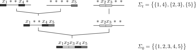
Figure 3.3. Determining the type of an individual at time $t$ via the partitioning process $(\varSigma_{\tau})_{0\leqslant\tau\leqslant t}$.

Theorem 3.2 (Solution of the recombination equation [3]).

The solution of the recombination equation (2.4) reads

$$\omega_{t}\,=\!\sum_{\mathcal{A}\in\hskip 0.5pt\mathcal{P}(S)}\!\!a_{t}(\mathcal{A})\,R_{\mathcal{A}}(\omega_{0})\,=\,\mathbb{E}\big{(}R_{\varSigma_{t}}(\omega_{0})\mid\varSigma_{0}=\boldsymbol{1}\big{)},$$

where

$$a_{t}(\mathcal{A})\,=\,\mathbb{P}\hskip 0.5pt\bigl{(}\varSigma_{t}=\mathcal{A}\mid\varSigma_{0}=\boldsymbol{1}\bigr{)}=(\hskip 0.5pt\mathrm{e}\hskip 0.5pt^{t\hskip 0.5ptQ})_{\boldsymbol{1}\mathcal{A}}$$

and $\mathbb{E}$ denotes expectation.

Remark 3.3.

With Theorem 3.2, we have found a stochastic representation of the solution of the (deterministic) differential equation (2.4). This reflects the fact that, while the time evolution of the composition of the infinite population follows a (dynamical) law of large numbers and is hence deterministic, the fate and ancestry of a single individual retains some stochasticity. While ancestral processes are common tools when working with the stochastic processes that describe finite populations, they are not within the usual scope of deterministic population genetics.

Remark 3.4.

In [3], the route of thought was, in fact, different from the one presented here. While we start from the ancestral process in this review, [3] works forward in time by means of classical methods from the theory of differential equations. The key was to establish the system of differential equations for the quantities $R_{\mathcal{A}}(\omega_{t})$, $\mathcal{A}\in\mathcal{P}(S)$, by exploiting the properties of the recombinators. This procedure mimics the algebraic technique of Haldane linearisation and leads to the generator $Q$ in a purely analytic way. The partitioning process then emerged as an interpretation of the result.

Remark 3.5.

It is easy to see that Theorem 3.2 extends to the duality relation

$$\mathbb{E}\big{(}R_{\mathcal{B}}(\omega_{t})\mid\omega_{0}=\nu\big{)}\,=\,\mathbb{E}\big{(}R_{\varSigma_{t}}(\nu)\mid\varSigma_{0}=\mathcal{B}\hskip 0.5pt\big{)}$$

for any $\nu\in\boldsymbol{P}(X)$ and $\mathcal{B}\in\mathcal{P}(S)$. Hence, since the left-hand side is deterministic,

$$R_{\mathcal{B}}(\omega_{t})\,=\,\mathbb{E}\big{(}R_{\varSigma_{t}}(\omega_{0})\mid\varSigma_{0}=\mathcal{B}\hskip 0.5pt\big{)}$$

for any initial condition $\omega_{0}\in\boldsymbol{P}(X)$.

Let us now turn to the evaluation of the $a_{t}$ of Theorem 3.2. It has been shown in [5] that, in the generic case that the $\psi^{\hskip 0.5ptU}\!(\mathcal{A})$ explained below are all distinct, it can be given in the form

(3.2) $$a_{t}(\mathcal{A})\,=\,\sum_{\underaccent{\text{.}}{\mathcal{B}\hskip 0.5pt}\succcurlyeq\mathcal{A}}\theta^{\hskip 0.5ptS}\!(\mathcal{A},\mathcal{B}\hskip 0.5pt)\,\hskip 0.5pt\mathrm{e}\hskip 0.5pt^{-\psi^{\hskip 0.5ptS}\!(\mathcal{B}\hskip 0.5pt)\hskip 0.5ptt}.$$

Here, the underdot denotes the summation variable, $\psi^{\hskip 0.5ptU}\!(\boldsymbol{1})\,\mathrel{\mathop{:}}=\,\sum_{\mathcal{A}\neq\boldsymbol{1}}\varrho^{U}\!(\mathcal{A})$ for all $\varnothing\neq U\subseteq S$, and the values for all other $\mathcal{A}\in\mathcal{P}(U)$ are defined recursively by $\psi^{\hskip 0.5ptU}\!(\mathcal{A})\,\mathrel{\mathop{:}}=\sum_{i=1}^{|\mathcal{A}|}\psi^{A_{i}}(\boldsymbol{1})\hskip 0.5pt.$ In the context of the partitioning process, $\psi^{A_{i}}(\boldsymbol{1})$ is the total rate of any further partitioning of part $A_{i}$, and so, due to the independence of the parts, $\psi^{\hskip 0.5ptU}\!(\mathcal{A})$ is the total rate of transitions out of state $\mathcal{A}$. The coefficients $\theta^{\hskip 0.5ptU}\!(\mathcal{A},\mathcal{B}\hskip 0.5pt)$ follow the recursion

(3.3) $$\theta^{\hskip 0.5ptU}\!(\mathcal{A},\mathcal{B}\hskip 0.5pt)\,=\!\sum_{\mathcal{B}\preccurlyeq\underaccent{\text{.}}{\mathcal{C}\hskip 0.5pt}\prec\boldsymbol{1}}\frac{\varrho^{U}\!(\mathcal{C})}{\psi^{\hskip 0.5ptU}\!(\boldsymbol{1})-\psi^{\hskip 0.5ptU}\!(\mathcal{B}\hskip 0.5pt)}\,\prod_{i=1}^{|\mathcal{C}|}\theta^{C_{i}}\big{(}\mathcal{A}|_{C_{i}},\mathcal{B}|_{C_{i}}\big{)}$$

for all $\mathcal{A}\preccurlyeq\mathcal{B}\prec\boldsymbol{1}$, where the initial conditions are given by $\theta^{\hskip 0.5ptU}\!(\boldsymbol{1},\boldsymbol{1})=1$ together with $\theta^{\hskip 0.5ptU}\!(\mathcal{A},\boldsymbol{1})\,=\,-\!\!\sum_{\mathcal{A}\preccurlyeq\underaccent{$\text{.}$}{\mathcal{C}\hskip 0.5pt}\prec\boldsymbol{1}}\!\theta^{\hskip 0.5ptU}\!(\mathcal{A},\mathcal{C})\hskip 0.5pt$ for $\mathcal{A}\prec\boldsymbol{1}$ and all $U\subseteq S$. Note that everything is uniquely determined by the initial conditions for the singleton sets $U=\{i\}$ with $i\in S$.

The recursion exploits the lower-triangular form of $Q$. This type of solution was motivated by earlier work of Geiringer [26], Bennett [13], Lyubich [32] and Dawson [19], who worked on the analogous system in discrete time (see below). We have made progress here by treating the problem within a systematic lattice-theoretic setting, which is the key for the transparent construction of the solution. Furthermore, the measure-theoretic framework allows to also work with more general type spaces, where the $X_{i}$ may be locally compact [3].

Let us note that the recursion (3.3) is of a fairly simple structure and computationally convenient. In the next section, we shall present an explicit solution for the special case of single-crossover recombination.

Remark 3.6.

Given the generator $Q$ from Proposition 3.1, the matrix function of transition probabilities, $M(t)\mathrel{\mathop{:}}=\hskip 0.5pt\mathrm{e}\hskip 0.5pt^{tQ}$, solves the Cauchy problem $\dot{M}=MQ$ with initial condition $M(0)=\mathbbm{1}$ (where $\mathbbm{1}$ is the identity matrix) and constitutes a Markov semigroup, so $M(t+s)=M(t)M(s)$ for $t,s\geqslant 0$. More generally, it is also of interest to consider the inhomogeneous counterpart, where $Q=Q(t)$ is time dependent; see [1, Addendum] for an example in the case of single crossovers. Let $M(t)$ again denote the solution of the Cauchy problem, which is unique under mild assumptions on $Q$ by general principles [22]. Clearly, $M(t)$ is still the matrix of transition probabilities until time $t$ and the underlying process satisfies the Markov property, while the semigroup property is lost.

There are now two scenarios to be distinguished as follows. When the generator family $(Q(t))_{t\geqslant 0}$ is commuting, so $Q(t)Q(s)=Q(s)Q(t)$ for all $t,s\geqslant 0$, one gets

(3.4) $$M(t)\,=\,\exp\int_{0}^{t}Q(\zeta)\hskip 0.5pt\mathrm{d}\hskip 0.5pt\zeta$$

or, more generally, $M(t,s)=\exp\int_{t}^{s}Q(\tau)\hskip 0.5pt\mathrm{d}\hskip 0.5pt\tau$, with $M(t,s)M(s,r)=M(t,r)$ for $r\geqslant s\geqslant t\geqslant 0$, also known as the flow property. In general, however, the generators $Q(t)$ need not commute, and Eq. (3.4) has to be replaced by the more general Peano–Baker formula; see [10] for details. It can still be evaluated in some simple cases, and the flow property remains valid.

Let us finally turn to the asymptotic behaviour of the solution of the recombination equation. It can, of course, be read off Eq. (3.2), but it is more instructive to argue directly on the grounds of $(\varSigma_{t})_{t\geqslant 0}$. The following consequence of Proposition 3.1 and Theorem 3.2 is then immediate.

Corollary 3.7 (Asymptotic behaviour of recombination equation).

Assume without loss of generality that $\varrho^{\{i,i+1\}}_{\{\{i\},\{i+1\}\}}>0$ for all $i\in S\setminus\{n\}$ $($if this is not the case, glue sites $i$ and $i+1$ together so that they form a single site$\hskip 0.5pt)$. The partitioning process is then absorbing, with

$$\lim_{t\to\infty}\varSigma_{t}\,=\,\big{\{}\{1\},\{2\},\ldots,\{n\}\big{\}}$$

almost surely and independently of $\varSigma_{0}$, and

$$\lim_{t\to\infty}\omega_{t}\,=\,\bigotimes_{i=1}^{n}(\pi_{i}.\omega_{0}).$$

The convergence to the limit is exponentially fast.

4. An explicit solution for single-crossover recombination

There is an important special case that allows for a closed solution of the Markov semigroup, beyond the somewhat deceptive notation $\hskip 0.5pt\mathrm{e}\hskip 0.5pt^{tQ}$ for the Markov semigroup generated by $Q$. This is the case of single crossovers of two parental gametes, which is also highly relevant biologically: Since crossovers are rare, it is unlikely that two or more of them happen in a given reproduction event, in any sequence of moderate length.

We speak of single-crossover recombination if $\varrho(\mathcal{A})>0$ implies $\mathcal{A}\!\in\!\mathcal{I}_{\leqslant 2}(S)$. Here, $\mathcal{I}(S)$ is the set of interval partitions of $S$, $\mathcal{I}_{\leqslant 2}(S)$ is the set of interval partitions of $S$ into at most two parts, and $\mathcal{I}_{2}(S)$ is the set of interval partitions of $S$ into exactly two parts. Clearly,

$$\mathcal{I}_{2}(S)=\{\mathcal{A}_{k}\,:\,1\leqslant k\leqslant n-1\}\hskip 0.5pt,$$

where $\mathcal{A}_{k}\mathrel{\mathop{:}}=\{\{1,2,\dotsc,k\},\{k+1,\dotsc,n\}\}$. The partition $\mathcal{A}_{k}$ is the result of a single-crossover event after site $k$. Obviously, there is a one-to-one correspondence between the elements of $\mathcal{I}_{2}(S)$ and those of $S\setminus\{n\}$.

Likewise, there is a one-to-one correspondence between $\mathcal{I}(S)$ and the set of subsets of $S\setminus\{n\}$. Let $G=\{j_{1},\ldots,j_{\lvert G\rvert}\}\subseteq S\setminus\{n\}$, with $j_{1}<j_{2}<\dots<j_{\lvert G\rvert}$. Let then $\mathcal{S}(\varnothing)=\boldsymbol{1}$, and, for $G\neq\varnothing$, let $\mathcal{S}(G)$ denote the interval partition

$$\mathcal{S}(G)\,\mathrel{\mathop{:}}=\,\bigl{\{}\{1,\ldots,j_{1}\},\{j_{1}+1,\ldots,j_{2}\},\ldots,\{j_{\lvert G\rvert}+1,\ldots,n\}\bigr{\}}\hskip 0.5pt.$$

In particular, ${\mathcal{S}}\big{(}S\setminus\{n\}\big{)}=\bigl{\{}\{0\},\ldots,\{n\}\bigr{\}}$. It is clear that ${\mathcal{S}}(H)\preccurlyeq{\mathcal{S}}(G)$ if and only if $G\subseteq H$. It is also obvious that $\mathcal{S}$ defines a bijection; its inverse,

(4.1) $$\varphi=\mathcal{S}^{-1},$$

associates with every interval partition of $S$ the corresponding subset of $S\setminus\{n\}$, so that $\varphi(\mathcal{S}(G))=G$ for all $G\subseteq S\setminus\{n\}$.

It is clear that $\mathcal{S}(G)$ may alternatively be represented as

(4.2) $$\mathcal{S}(G)\,=\,\boldsymbol{1}\wedge\mathcal{A}_{j_{1}}\wedge\mathcal{A}_{j_{2}}\wedge\ldots\wedge\mathcal{A}_{j_{\lvert G\rvert}}\hskip 0.5pt,$$

where $\wedge$ denotes the coarsest common refinement; note that the action of $\wedge$ is commutative. In particular, one has $\mathcal{S}\big{(}G\cup\{k\}\big{)}=\mathcal{S}(G)\wedge\mathcal{A}_{k}$. More precisely, let $\mathcal{S}(G)=\mathcal{B}=\{B_{1},\ldots,B_{m}\}$ and $k\in S\setminus\{n\}$. Then,

$$\mathcal{B}\wedge\mathcal{A}_{k}=\begin{cases}\mathcal{B},&k\in G\hskip 0.5pt,\\ (\mathcal{B}\setminus B_{i})\cup\mathcal{A}_{k}|_{B_{i}},&k\in S\setminus\big{(}G\cup\{n\}\big{)}\hskip 0.5pt,\end{cases}$$

where, in the latter case, $B_{i}$ is the unique block that contains $k$; the other blocks are not affected.

Let us now connect this to the partitioning process. Assume that we have $\varSigma_{\tau}=\mathcal{B}=\{B_{1},\ldots,B_{m}\}=\mathcal{S}(G)$ for some $G\subseteq S\setminus\{n\}$ and fix one index $1\leqslant i\leqslant m$. Evaluating the rates in Proposition 3.1 with the help of the marginal recombination rates (3.1) then reveals that, in the single-crossover case, the only (non-silent) transitions involving block $B_{i}$ are

$$\begin{split}&\mathcal{B}\>\mapsto\>(\mathcal{B}\setminus B_{i})\cup\mathcal{A}_{k}|_{B_{i}}\,=\,\mathcal{B}\wedge\mathcal{A}_{k},\\ &\text{at rate }\varrho(\mathcal{A}_{k})\text{ for all }k\in B_{i}\setminus\big{(}G\cup\{n\}\big{)}\,.\end{split}$$

If all blocks are taken into account, we therefore get the transitions

(4.3) $$\begin{split}&\mathcal{S}(G)=\mathcal{B}\>\mapsto\>\mathcal{B}\wedge\mathcal{A}_{k}=\mathcal{S}\big{(}G\cup\{k\}\big{)},\\ &\text{at rate }\varrho(\mathcal{A}_{k})\text{ for all }k\in S\setminus\big{(}G\cup\{n\}\big{)}.\end{split}$$

Since $\mathcal{S}\big{(}G\cup\{k\}\big{)}$ is again an interval partition, it is clear that $\{\varSigma_{\tau}\}_{\tau\geqslant 0}$, when started in $\mathcal{I}(S)$, will never leave $\mathcal{I}(S)$.

Remark 4.1.

The property that recombination according to $\mathcal{A}$ induces the transition from $\mathcal{B}$ to $\mathcal{B}\wedge\mathcal{A}$ is a special (and decisive) property of the single-crossover setting, where $\mathcal{A}\in\mathcal{I}_{\leqslant 2}(S)$ and $\mathcal{B}\in\mathcal{I}(S)$, which implies that $\mathcal{A}$ refines at most one block of $\mathcal{B}$. This is not true in the general case, where the possible refinements are considerably more complex.

We are now well prepared to calculate $a_{t}$. We could work via the matrix exponential of $Q$ and use its special structure resulting from the restriction to $\mathcal{I}(S)$; however, we pursue a more elegant approach based on Eqs. (4.2) and (4.3). To this end, let $\varSigma_{0}=\boldsymbol{1}$ and conclude from Eq. (4.3) that $(\varSigma_{\tau})_{\tau\geqslant 0}$ is governed by the arrival of $\mathcal{A}_{k}$-events that happen independently of each other at rate $\varrho(\mathcal{A}_{k})$. The waiting times $T_{k}$ until $\mathcal{A}_{k}$ appears are therefore independent and exponentially distributed with parameters $\varrho(\mathcal{A}_{k})$. Let now $\mathcal{C}$ be an interval partition as in Eq. (4.2), that is, $\mathcal{C}=\mathcal{S}(G)$ for some $G\subseteq S\setminus\{n\}$ (so $G=\varphi(\mathcal{C})$). Taking Eqs. (4.2) and (4.3) together, we see that $\varSigma_{t}=\mathcal{C}$ if and only if all $\mathcal{A}_{k}$-events with $k\in G$ have occurred, while all $\mathcal{A}_{j}$-events with $j\in S\setminus\big{(}G\cup\{n\}\big{)}$ have not. We therefore get

$$\begin{split}a_{t}(\mathcal{C})&=\,\mathbb{P}\hskip 0.5pt(\varSigma_{t}=\mathcal{C}\mid\varSigma_{0}=\boldsymbol{1})\,=\,\prod_{k\in G}\mathbb{P}\hskip 0.5pt\big{(}T_{k}<t\big{)}\prod_{\ell\in S\setminus(G\cup\{n\})}\mathbb{P}\hskip 0.5pt\big{(}T_{\ell}\geqslant t\big{)}\\ &=\,\prod_{k\in G}\big{(}1-\hskip 0.5pt\mathrm{e}\hskip 0.5pt^{-t\varrho(\mathcal{A}_{k})}\big{)}\prod_{\ell\in S\setminus(G\cup\{n\})}\hskip 0.5pt\mathrm{e}\hskip 0.5pt^{-t\varrho(\mathcal{A}_{\ell})}\hskip 0.5pt.\end{split}$$

With these coefficients, Theorem 3.2 indeed turns into an explicit and simple solution of the recombination equation. Let us summarise our result as follows.

Corollary 4.2 (Single-crossover recombination).

Assume single-crossover recombination, that is, $\varrho(\mathcal{A})>0$ implies $\mathcal{A}\in\mathcal{I}_{\leqslant 2}(S)$. The probability vector $a_{t}$ from Theorem 3.2 is then given by $a_{t}(\mathcal{C})=0$ if $\mathcal{C}\notin\mathcal{I}(S)$ and, for $\mathcal{C}\in\mathcal{I}(S)$, by

$$a_{t}(\mathcal{C})\,=\,\prod_{k\in G}\big{(}1-\hskip 0.5pt\mathrm{e}\hskip 0.5pt^{-t\varrho(\mathcal{A}_{k})}\big{)}\prod_{\ell\in S\setminus(G\cup\{n\})}\hskip 0.5pt\mathrm{e}\hskip 0.5pt^{-t\varrho(\mathcal{A}_{\ell})}\hskip 0.5pt,$$

where $G=\varphi(\mathcal{C})$ of Eq. (4.1).

In fact, the content of Corollary 4.2 was originally obtained by analytic means in [2]; we have recovered it here in genealogical terms. Note that the exponential convergence to the product measure of Corollary 3.7 is obvious here from the explicit formula for the $a_{t}(\mathcal{C})$.

5. Recombination in discrete time

Let us finally turn our attention to the discrete-time analogue of Eq. (2.4), namely the discrete-time dynamical system

(5.1) $$\omega_{t+1}\,=\!\sum_{\mathcal{A}\in\mathcal{P}_{\!\leqslant 2}(S)}\!r(\mathcal{A})\,R_{\mathcal{A}}(\omega_{t})\hskip 0.5pt,$$

which is often considered in population genetics [16, 19, 32, 33]. Here, $t\in\mathbb{N}_{0}$ now denotes discrete time (counting generations); the initial condition is again $\omega_{0}\in\boldsymbol{P}(X)$. The iteration describes the synchronous formation of a new population from the parental one. The parameters are now the recombination probabilities $r(\mathcal{A})$ for $\mathcal{A}\in\mathcal{P}_{\!\leqslant 2}(S)$. Obviously, $\omega_{t+1}$ is a convex combination of $\omega_{t}$ recombined in all possible ways, so $\boldsymbol{P}(X)$ is preserved under the iteration.

In analogy with the derivation of the continuous-time recombination equation as the limit of a finite-$N$ Moran model, the discrete-time recombination equation may be obtained as the law of large numbers of an underlying Wright–Fisher model with recombination; see [9] for the special case of single crossovers. Rather than working this out explicitly, we simply state the plausible fact that there is again an underlying partitioning process, $(\varSigma_{\tau})_{\tau\in\mathbb{N}_{0}}$. This is now a Markov chain in discrete time, again with values in $\mathcal{P}(S)$ and starting at $\varSigma_{0}=\boldsymbol{1}$. When $\varSigma_{\tau}=\mathcal{A}$, in the time step from $\tau$ to $\tau+1$, part $A$ of $\mathcal{A}$ is replaced by $\mathfrak{a}\in\mathcal{P}(A)$ with probability $r^{A}(\mathfrak{a})$, independently for each $A\in\mathcal{A}$. Note that, in contrast to the continuous-time case, several parts can be refined at the same time, which makes the discrete-time case actually more complicated. Of course, $\mathfrak{a}=\{A\}$, which means no action on this part, is also possible. Put together, it is not difficult to verify that one ends up with the Markov transition matrix $M$ with elements

$$M_{\mathcal{A}\mathcal{B}}\,=\,\begin{cases}\prod_{A\in\mathcal{A}}r^{A}(\mathcal{B}|_{A}),&\text{if }\mathcal{B}\preccurlyeq\mathcal{A},\\ 0,&\text{otherwise}.\end{cases}$$

In particular, $M=\bigl{(}M_{\mathcal{A}\mathcal{B}}\bigr{)}_{\mathcal{A},\mathcal{B}\in\mathcal{P}(S)}$ is a lower-triangular Markov matrix. (Let us note in passing that the triangular form, which also appears in the continuous-time case, motivated to revisit the Markov embedding problem [12].) The analogue of Theorem 3.2 reads as follows.

Theorem 5.1 (Solution of the discrete-time recombination equation [3]).

The solution of the recombination equation (5.1) is given by

(5.2) $$\omega_{t}\,=\!\sum_{\mathcal{A}\in\hskip 0.5pt\mathcal{P}(S)}\!\!a_{t}(\mathcal{A})\,R_{\mathcal{A}}(\omega_{0})\,=\,\mathbb{E}\big{(}R_{\varSigma_{t}}(\omega_{0})\mid\varSigma_{0}=\boldsymbol{1}\big{)},$$

where

$$a_{t}(\mathcal{A})\,=\,\mathbb{P}\hskip 0.5pt\bigl{(}\varSigma_{t}=\mathcal{A}\mid\varSigma_{0}=\boldsymbol{1}\bigr{)}=(M^{t})_{\boldsymbol{1}\mathcal{A}}.$$

It is tempting to assume that, again in analogy with continuous time, the case with single crossovers might be amenable to a simple solution. This is, however, not true. The reason is that, in continuous time, the single-crossover events appear independently by the very nature of the continuous-time process, where the probability of two events occurring simultaneously is zero. In contrast, the single-crossover assumption in discrete time induces dependence. Namely, a crossover between a given pair of neighbouring sites precludes a crossover between another pair of neighbouring sites in the same block. With the help of Möbius inversion on a suitable poset of rooted forests, a solution was obtained nevertheless, but it is of surprising complexity [6]. However, the long-term behaviour is, once more, simple: Corollary 3.7 carries over, with $\varrho$ replaced by $r$.

Acknowledgements

It is our pleasure to thank Frederic Alberti for critically reading the manuscript, and two referees for helpful comments.

References

- [1] M. Baake, Recombination semigroups on measure spaces, Monatsh. Math. 146 (2005), 267–278; and 150 (2007), 83–84 (addendum).
- [2] M. Baake and E. Baake, An exactly solved model for mutation, recombination and selection, Can. J. Math. 55 (2003), 3–41; and 60 (2008), 264–265 (erratum).
- [3] E. Baake and M. Baake, Haldane linearisation done right: Solving the nonlinear recombination equation the easy way, Discr. Cont. Dynam. Syst. A 36 (2016), 6645–6656.
- [4] E. Baake, F. Cordero, and S. Hummel, A probabilistic view on the deterministic mutation–selection equation: dynamics, equilibria, and ancestry via individual lines of descent, J. Math. Biol. 77 (2018), 795–820.
- [5] E. Baake, M. Baake, and M. Salamat, The general recombination equation in continuous time and its solution, Discr. Cont. Dynam. Syst. A 36 (2016), 63–95; and 36 (2016), 2365–2366 (erratum and addendum).
- [6] E. Baake and M. Esser, Fragmentation process, pruning poset for rooted forests, and Möbius inversion, Markov Proc. Rel. Fields 24 (2018), 57–84.
- [7] E. Baake and I. Herms, Single-crossover dynamics: Finite versus infinite populations, Bull. Math. Biol. 70 (2008), 603–624.
- [8] E. Baake and A. Wakolbinger, Lines of descent under selection, J. Stat. Phys. 172 (2018), 156–174.
- [9] E. Baake and U. von Wangenheim, Single-crossover recombination and ancestral recombination trees, J. Math. Biol. 68 (2014), 1371–1402.
- [10] M. Baake and U. Schlägel, The Peano–Baker series, Proc. Steklov Inst. Math. 275 (2011), 167–171.
- [11] M. Baake and E. Shamsara, The recombination equation for interval partitions, Monatsh. Math. 182 (2017), 243–269.
- [12] M. Baake and J. Sumner, Notes on Markov embedding, Lin. Alg. Appl., in press; arxiv:1903.08736.
- [13] J. H. Bennett, On the theory of random mating, Ann. Human Genetics 18 (1954), 311–317.
- [14] A. Bhaskar and Y.S. Song, Closed-form asymptotic sampling distributions under the coalescent with recombination for an arbitrary number of loci, Adv. Appl. Prob. 44 (2012), 391–407.
- [15] A. Bobrowski, T. Wojdyła and M. Kimmel, Asymptotic behavior of a Moran model with mutations, drift and recombination among multiple loci, J. Math. Biol. 61 (2010), 455–473.
- [16] R. Bürger, The Mathematical Theory of Selection, Recombination, and Mutation, Wiley, Chichester, 2000.
- [17] F.B. Christiansen, Population Genetics of Multiple Loci, Wiley, Chichester, 1999.
- [18] F. Cordero, Common ancestor type distribution: A Moran model and its deterministic limit, Stoch. Proc. Appl. 127 (2017), 590–621.
- [19] K.J. Dawson, The evolution of a population under recombination: How to linearise the dynamics, Lin. Alg. Appl. 348 (2002), 115–137.
- [20] R. Durrett, Probability Models for DNA Sequence Evolution, 2nd ed., Springer, New York, 2008.
- [21] J.-Y. Dutheil, Towards more realistic models of genomes in populations: the Markov-modulated sequentially Markov coalescent, in Probabilistic Structures in Evolution, E. Baake and A. Wakolbinger (eds.), EMS Publishing House, Zurich, in press.
- [22] K.-J. Engel and R. Nagel, One-Parameter Semigroups for Linear Evolution Equations, Springer, New York, 2000.
- [23] M. Esser, S. Probst and E. Baake, Partitioning, duality, and linkage disequilibria in the Moran model with recombination, J. Math. Biol. 73 (2016), 161–197.
- [24] M. Esser, Recombination Models Forward and Backward in Time, PhD thesis, Bielefeld University, 2017, urn:nbn:de:0070-pub-29102790.
- [25] S.N. Ethier and T.G. Kurtz, Markov Processes: Characterization and Convergence, Wiley, New York, 1986, reprint 2005.
- [26] H. Geiringer, On the probability theory of linkage in Mendelian heredity, Ann. Math. Stat. 15 (1944), 25–57.
- [27] R.C. Griffiths and R. Marjoram, Ancestral inference from samples of DNA sequences with recombination, J. Comput. Biol. 3 (1996), 479–502.
- [28] R.R. Hudson, Properties of an neutral allele model with intragenetic recombination, Theor. Popul. Biol. 23 (1983), 183–201.
- [29] D. McHale and G.A. Ringwood, Haldane linearisation of baric algebras, J. London Math. Soc. (2) 28 (1983), 17–26.
- [30] J. Hein, M.H. Schierup and C. Wiuf, Gene Genealogies, Variation and Evolution: A Primer in Coalescent Theory, Oxford University Press, Oxford, 2005.
- [31] H.S. Jennings, The numerical results of diverse systems of breeding, with respect to two pairs of characters, linked or independent, with special relation to the effects of linkage, Genetics 2 (1917), 97–154.
- [32] Y. I. Lyubich, Mathematical Structures in Population Genetics, Springer, Berlin, 1992.
- [33] S. Martínez, A probabilistic analysis of a discrete-time evolution in recombination, Adv. Appl. Math. 91 (2017), 115–136.
- [34] T. Ohta and M. Kimura, Linkage disequilibrium due to random genetic drift, Genet. Res. 13 (1969), 47–55.
- [35] R.B. Robbins, Some applications of mathematics to breeding problems III. Genetics 3 (1918), 375–389.
- [36] Y.S. Song and J.S. Song, Analytic computation of the expectation of the linkage disequilibrium coefficient , Theor. Popul. Biol. 71 (2007), 49–60.
- [37] J. Wakeley, Coalescent Theory: An Introduction, Roberts and Co., Greenwood Village, CO, 2009.