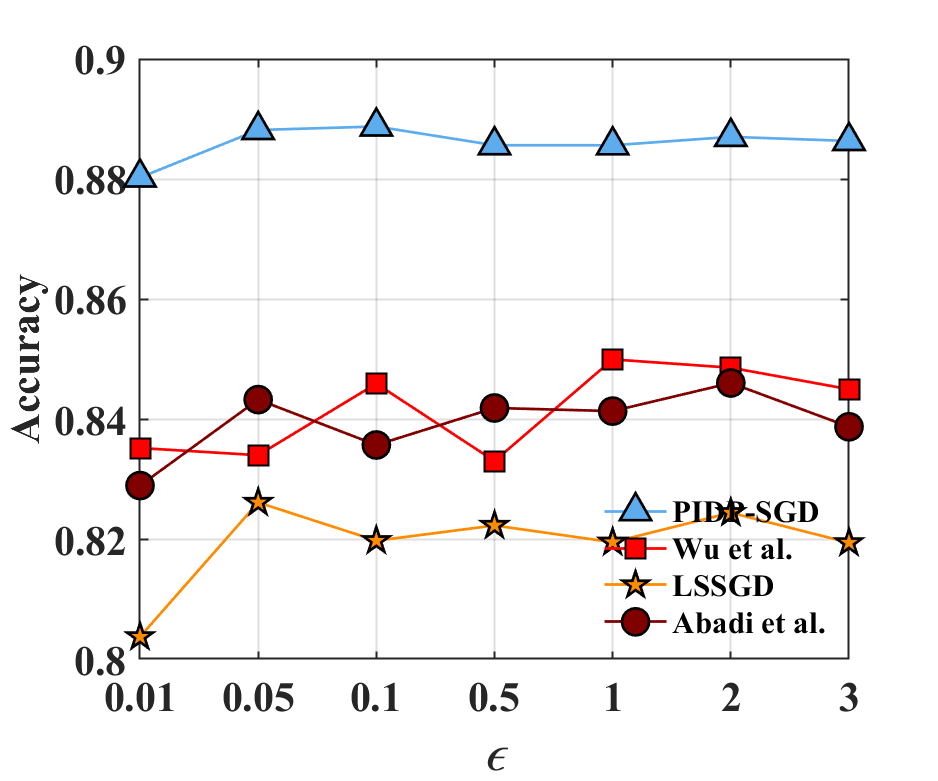
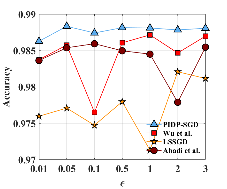
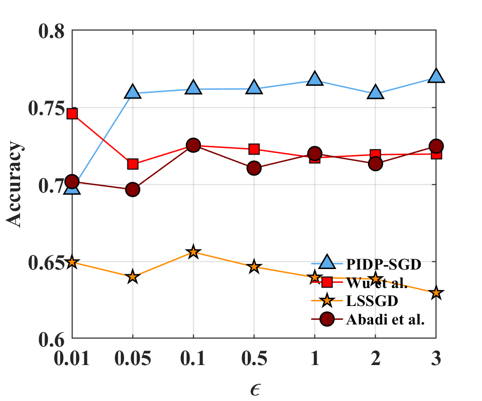
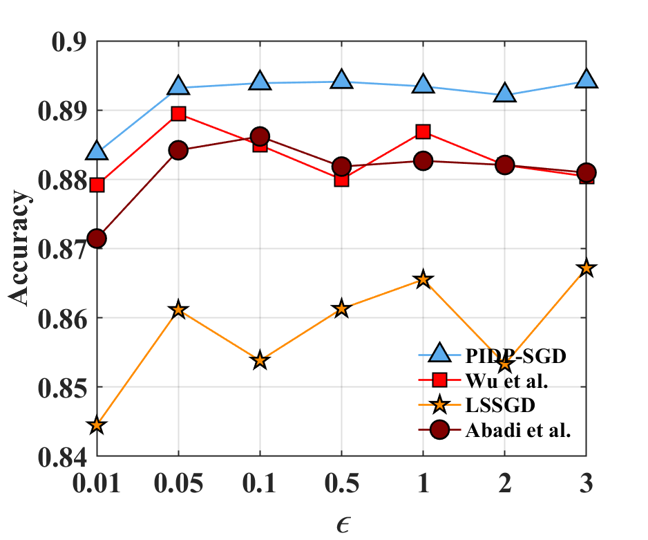
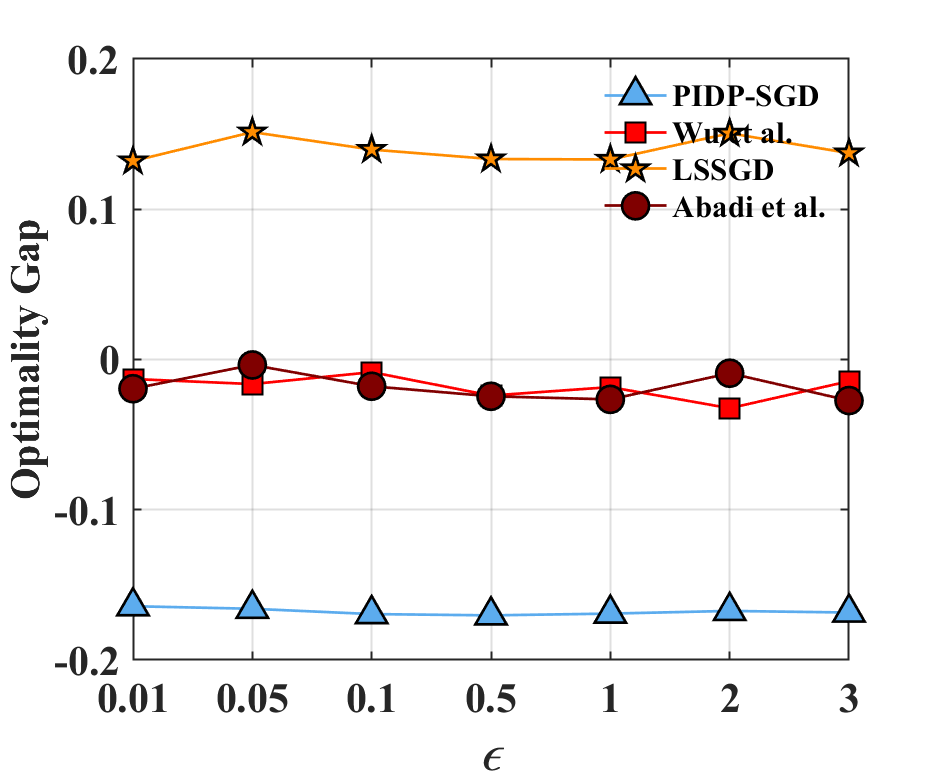
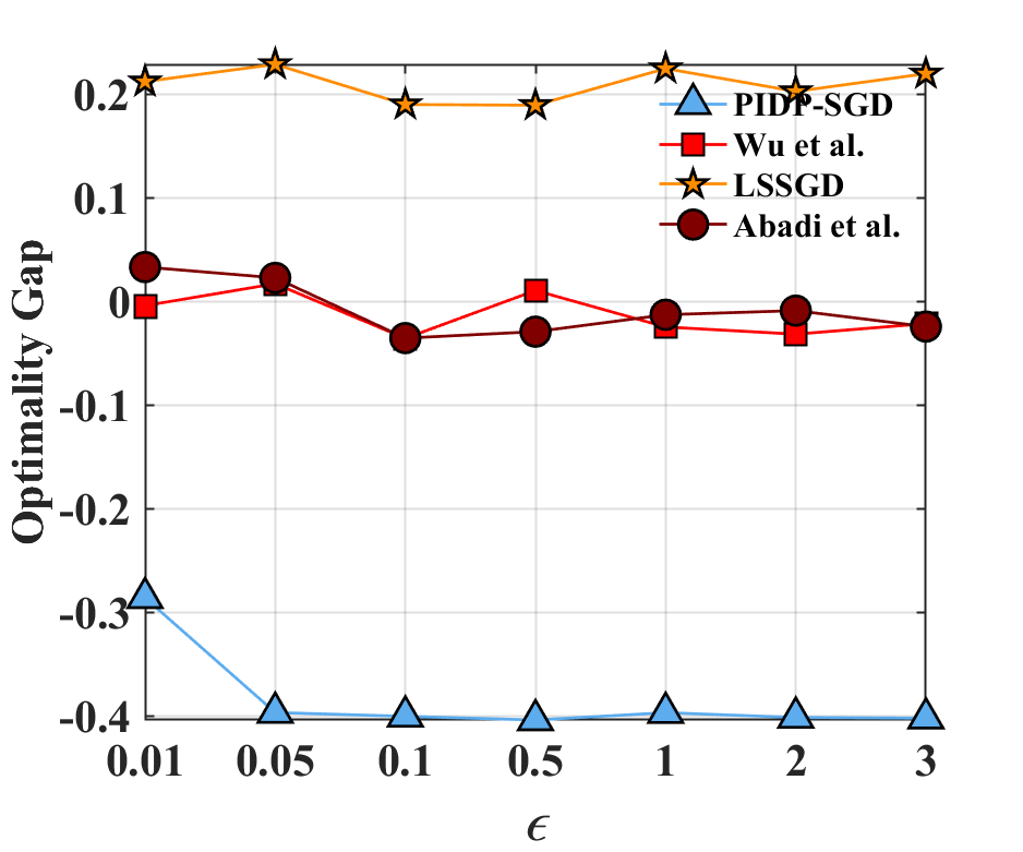
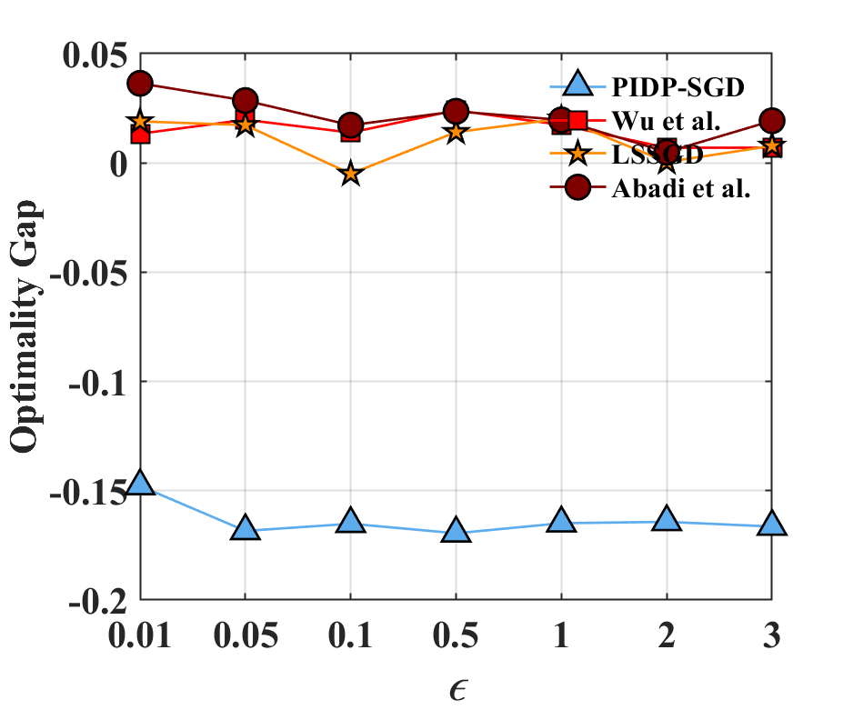
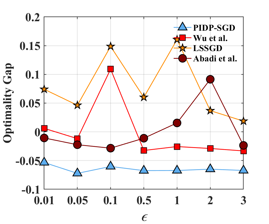
11institutetext: Institute of Information Engineering, Chinese Academy of Sciences 11email: {kangyilin,lijian9026,wangweiping}@iie.ac.cn
22institutetext: Gaoling School of Artificial Intellignece, Renmin University of China 22email: liuyonggsai@ruc.edu.cn
33institutetext: School of Cyber Security, University of Chinese Academy of Sciences

Data Heterogeneity Differential Privacy: From Theory to Algorithm thanks: This work was supported in part by the Excellent Talents Program of Institute of Information Engineering, CAS, the Special Research Assistant Project of CAS, the Beijing Outstanding Young Scientist Program (No. BJJWZYJH012019100020098), Beijing Natural Science Foundation (No. 4222029), and National Natural Science Foundation of China (No. 62076234, No. 62106257).

Yilin Kang 1133    Jian Li 11    Yong Liu 22    Weiping Wang 11
Abstract

Traditionally, the random noise is equally injected when training with different data instances in the field of differential privacy (DP). In this paper, we first give sharper excess risk bounds of DP stochastic gradient descent (SGD) method. Considering most of the previous methods are under convex conditions, we use Polyak-Łojasiewicz condition to relax it in this paper. Then, after observing that different training data instances affect the machine learning model to different extent, we consider the heterogeneity of training data and attempt to improve the performance of DP-SGD from a new perspective. Specifically, by introducing the influence function (IF), we quantitatively measure the contributions of various training data on the final machine learning model. If the contribution made by a single data instance is so little that attackers cannot infer anything from the model, we do not add noise when training with it. Based on this observation, we design a ‘Performance Improving’ DP-SGD algorithm: PIDP-SGD. Theoretical and experimental results show that our proposed PIDP-SGD improves the performance significantly.

Keywords:
Differential privacy Machine learning Data heterogeneity.

1 Introduction

Machine learning has been widely applied to many fields in recent decades and tremendous data has been collected. As a result, information disclosure becomes a huge problem. Except for the original data, model parameters can reveal sensitive information in an undirect way as well [17, 34].

Differential privacy (DP) [14, 15] is a theoretically rigorous tool to prevent sensitive information [10]. It preserves privacy by introducing random noise, to block adversaries from inferring any single individual included in the dataset by observing the machine learning model. As such, DP has attracted many researchers and has been applied to numerous machine learning methods [33, 50, 6, 42, 19, 46, 38, 2]. Some kind of attacks, such as membership inference attack, attribute inference attack, memorization attack, can be thwarted by differential privacy [3, 7, 21]. Empirical risk minimization (ERM), a popular optimization method that covers a variety of machine learning tasks, also faces privacy problems. A long list of works focuses on applying differential privacy to ERM [9, 23, 35, 5, 43, 47, 32, 44, 39], in which three main approaches are studied: output perturbation, objective perturbation, and gradient perturbation. Although there are wildspread researches these years, some problems still exist: Firstly, all data is usually treated equally when training DP model. However, in real scenarios, different training data affects the model differently, so treating them all the same lacks ‘common sense’ and is one of the reasons why low accuracy appears. Meanwhile, previous results always require that the loss function is convex (or even strongly convex), so the application scenario is narrow. Besides, existed excess risk bounds for non-convex setting is unsatisfactory.

To solve the problems, we make the following contributions in this paper: First, we introduce the Polyak-Łojasiewicz condition [22] to relax the convex (strongly convex) assumption. We analyze the excess empirical risk, the generalization error, the excess population risk and give corresponding bounds under this assumption. Theoretical results show that our given excess risk bounds are better than previous non-convex ones and even better than some of the convex ones. Second, motivated by the definition of DP, we provide a new perspective to improve the performance: treating different data instances differently. In particular, we introduce the Influence Function (IF) [24] to measure the contributions made by different data instances. If the data instance z𝑧z contributes so little to the machine learning model that the attacker cannot infer anything (represented by the privacy budget ϵitalic-ϵ\epsilon in DP), we do not add noise when training with z𝑧z, rather than treating all of the data instances as being the same. In this way, we propose a ‘Performance Improving’ algorithm: PIDP-SGD method to improve the model performance, by taking data heterogeneity into account.

The rest of the paper is organized as follows. First, we introduce some related work in Section 2. Preliminaries are presented in Section 3. We analyze the excess risk bounds of traditional DP-SGD method and give sharper theoretical bounds in Section 4. The ‘Performance Improving’ DP-SGD algorithm is given and analyzed in Section 5. In Section 6, we compare our proposed method with previous methods in detail. The experimental results are shown in 7. Finally, we conclude the paper in Section 8.

2 Related Work

The first method on DP-ERM is proposed in [9], in which output and objective perturbation methods are introduced. Gradient perturbation is proposed in [35], in which DP-SGD is analyzed for the first time. The accuracy of the objective perturbation method is improved by [23]. The excess empirical risk bounds of the methods proposed in [9] and [23] are improved by [5]. An output perturbation method is introduced to DP-SGD in [44], in which a novel 2subscript2\ell_{2} sensitivity of SGD is analyzed and better accuracy is achieved. [43] introduces Prox-SVRG [45] to DP and proposes DP-SVRG, in which optimal or near-optimal utility bounds are achieved.

Meanwhile, there are also some works concentrated on non-convex analysis. DP is introduced to deep learning by [1], via gradient perturbation method, however, it focuses on the privacy but lacks utility analysis. An output perturbation method is proposed in [47] under non-convex condition. The Polyak-Łojasiewicz condition is introduced in [43] and the excess empirical risk of gradient perturbation method under non-convex condition is analyzed, however, the excess population risk is not discussed. Aiming to achieve better performance, in [32], more noise is added to those features less ‘relevant’ to the final model. A Laplace smooth operator is introduced to DP-SGD and a new method: DP-LSSGD is proposed in [39], focusing on non-convex analysis. The excess empirical risk bound and the excess population risk bound of DP model under non-convex condition are analyzed by [41], via Gradient Langevin Dynamics. For non-convex condition, the theoretical results are always unsatisfactory.

All the works mentioned above are based on three traditional perturbation methods, all data instances are treated equally, which lacks ‘common sense’ and leads unsatisfactory utility. To solve the problems under both convex and non-convex conditions, we take data heterogeneity into account and propose a ‘Performance Improving’ algorithm. In this way, our method improves the performance of the DP model, which is superior to previous methods in the excess risk bounds.

3 Preliminaries

3.1 Notations and Assumptions

The loss function is defined as :𝒞×𝒟:𝒞𝒟\ell:\mathcal{C}\times\mathcal{D}\rightarrow\mathbb{R}, where 𝒞𝒞\mathcal{C} is the parameter space and 𝒟𝒟\mathcal{D} is the data universe. We assume that the parameter space is bounded, whose radius is r𝑟r. Supposing there are n𝑛n data instances in the dataset D={z1,,zn}𝒟n𝐷subscript𝑧1subscript𝑧𝑛superscript𝒟𝑛D=\{z_{1},\cdots,z_{n}\}\in\mathcal{D}^{n}, where zisubscript𝑧𝑖z_{i} are drawn i.i.d from the underlying distribution 𝒫𝒫\mathcal{P}. Besides, for each z=(x,y)𝑧𝑥𝑦z=(x,y), x𝑥x is the feature and y𝑦y is the label. We assume x21subscriptnorm𝑥21\|x\|_{2}\leq 1, i.e. 𝒳𝒳\mathcal{X} is the unit ball. Moreover, for a vector x=[x1,,xd]𝑥subscript𝑥1subscript𝑥𝑑x=[x_{1},\cdots,x_{d}], its 2subscript2\ell_{2} norm is defined as: x2=(i=1dxi2)1/2subscriptnorm𝑥2superscriptsuperscriptsubscript𝑖1𝑑superscriptsubscript𝑥𝑖212\|x\|_{2}=\big{(}\sum_{i=1}^{d}x_{i}^{2}\big{)}^{1/2}, and the ithsuperscript𝑖𝑡i^{th} element xisubscript𝑥𝑖x_{i} is represented by [x]isubscriptdelimited-[]𝑥𝑖[x]_{i}. In the following, we use subscript\nabla_{\cdot} to denote the gradient over \cdot.

In ERM, our goal is to find the optimal model that minimizes the empirical risk L(θ;D)=1ni=1n(θ,zi)𝐿𝜃𝐷1𝑛superscriptsubscript𝑖1𝑛𝜃subscript𝑧𝑖L(\theta;D)=\frac{1}{n}\sum_{i=1}^{n}\ell\big{(}\theta,z_{i}\big{)} on dataset D𝐷D, defined as: θ=argmin[L(θ;D)]superscript𝜃𝐿𝜃𝐷\theta^{*}=\arg\min\big{[}L\big{(}\theta;D\big{)}\big{]}, and L(θ;D)𝐿superscript𝜃𝐷L(\theta^{*};D) is represented by Lsuperscript𝐿L^{*}. Additionally, the population risk is defined as L𝒫(θ)=𝔼z𝒫[(θ,z)]subscript𝐿𝒫𝜃subscript𝔼similar-to𝑧𝒫delimited-[]𝜃𝑧L_{\mathcal{P}}\big{(}\theta\big{)}=\mathbb{E}_{z\sim\mathcal{P}}\big{[}\ell\big{(}\theta,z\big{)}\big{]}. For an algorithm 𝒜:𝒟nm:𝒜superscript𝒟𝑛superscript𝑚\mathcal{A}:\mathcal{D}^{n}\rightarrow\mathbb{R}^{m}, we denote its output as θ𝒜subscript𝜃𝒜\theta_{\mathcal{A}}. The excess empirical risk denotes the gap between θ𝒜subscript𝜃𝒜\theta_{\mathcal{A}} and θsuperscript𝜃\theta^{*}, defined as: L(θ𝒜;D)L𝐿subscript𝜃𝒜𝐷superscript𝐿L(\theta_{\mathcal{A}};D)-L^{*}; and the excess population risk represents the gap between θ𝒜subscript𝜃𝒜\theta_{\mathcal{A}} and the optimal model over the underlying 𝒫𝒫\mathcal{P}, defined as: L𝒫(θ𝒜)minθ𝒞L𝒫(θ)subscript𝐿𝒫subscript𝜃𝒜subscript𝜃𝒞subscript𝐿𝒫𝜃L_{\mathcal{P}}(\theta_{\mathcal{A}})-\min_{\theta\in\mathcal{C}}L_{\mathcal{P}}(\theta). The generalization error connects the population risk and the empirical risk, defined as: L𝒫(θ𝒜)L(θ𝒜;D)subscript𝐿𝒫subscript𝜃𝒜𝐿subscript𝜃𝒜𝐷L_{\mathcal{P}}(\theta_{\mathcal{A}})-L(\theta_{\mathcal{A}};D).

Besides, there are some assumptions on the loss function:

Definition 1 (G𝐺G-Lipschitz)

A loss function :𝒞×𝒟:𝒞𝒟\ell:\mathcal{C}\times\mathcal{D}\rightarrow\mathbb{R} is G𝐺G-Lipschitz over θ𝜃\theta, if for some constant G𝐺G, any z𝒟𝑧𝒟z\in\mathcal{D} and θ,θ𝒞𝜃superscript𝜃𝒞\theta,\theta^{\prime}\in\mathcal{C}, we have: |(θ,z)(θ,z)|Gθθ2𝜃𝑧superscript𝜃𝑧𝐺subscriptnorm𝜃superscript𝜃2|\ell(\theta,z)-\ell(\theta^{\prime},z)|\leq G\|\theta-\theta^{\prime}\|_{2}.

Definition 2 (L𝐿L-smooth)

A loss function :𝒞×𝒟:𝒞𝒟\ell:\mathcal{C}\times\mathcal{D}\rightarrow\mathbb{R} is L𝐿L-smooth over θ𝜃\theta, if for some constant L𝐿L, any z𝒟𝑧𝒟z\in\mathcal{D} and θ,θ𝒞𝜃superscript𝜃𝒞\theta,\theta^{\prime}\in\mathcal{C}, we have: θ(θ,z)θ(θ,z)2Lθθ2subscriptnormsubscript𝜃𝜃𝑧subscript𝜃superscript𝜃𝑧2𝐿subscriptnorm𝜃superscript𝜃2\|\nabla_{\theta}\ell(\theta,z)-\nabla_{\theta}\ell(\theta^{\prime},z)\|_{2}\leq L\|\theta-\theta^{\prime}\|_{2}.

Definition 3 (C𝐶C-Hessian Lipschitz)

A loss function :𝒞×𝒟:𝒞𝒟\ell:\mathcal{C}\times\mathcal{D}\rightarrow\mathbb{R} is C𝐶C-Hessian Lipschitz over θ𝜃\theta, if for any z𝒟𝑧𝒟z\in\mathcal{D} and θ,θ𝒞𝜃superscript𝜃𝒞\theta,\theta^{\prime}\in\mathcal{C}, we have: θ2(θ,z)θ2(θ,z)2Cθθ2subscriptnormsubscriptsuperscript2𝜃𝜃𝑧subscriptsuperscript2𝜃superscript𝜃𝑧2𝐶subscriptnorm𝜃superscript𝜃2\|\nabla^{2}_{\theta}\ell(\theta,z)-\nabla^{2}_{\theta}\ell(\theta^{\prime},z)\|_{2}\leq C\|\theta-\theta^{\prime}\|_{2}.

Remark 1

G𝐺G-Lipschitz means that θ(θ,z)2Gsubscriptnormsubscript𝜃𝜃𝑧2𝐺\|\nabla_{\theta}\ell(\theta,z)\|_{2}\leq G. For Mean Squared Error, elements in θ(θ,z)subscript𝜃𝜃𝑧\nabla_{\theta}\ell(\theta,z) are less than 2c2𝑐2c if yf(x)𝑦𝑓𝑥y-f(x)111f(x)𝑓𝑥f(x) is a general notation, for example, f(x)=θTx𝑓𝑥superscript𝜃𝑇𝑥f(x)=\theta^{T}x in linear regression. is bounded by c𝑐c. For logistic regression over cross entropy, elements in θ(θ,z)subscript𝜃𝜃𝑧\nabla_{\theta}\ell(\theta,z) are less than 1. L𝐿L-smooth means that θ2(θ,z)2Lsubscriptnormsuperscriptsubscript𝜃2𝜃𝑧2𝐿\|\nabla_{\theta}^{2}\ell(\theta,z)\|_{2}\leq L. For Mean Squared Error, elements in θ2(θ,z)subscriptsuperscript2𝜃𝜃𝑧\nabla^{2}_{\theta}\ell(\theta,z) are less than 2. For logistic regression over cross entropy, elements in θ2(θ,z)subscriptsuperscript2𝜃𝜃𝑧\nabla^{2}_{\theta}\ell(\theta,z) are less than 0.25. C𝐶C-Hessian Lipschitz means that θ3(θ,z)2Csubscriptnormsuperscriptsubscript𝜃3𝜃𝑧2𝐶\|\nabla_{\theta}^{3}\ell(\theta,z)\|_{2}\leq C. For Mean Squared Error, θ3(θ,z)2=0subscriptnormsubscriptsuperscript3𝜃𝜃𝑧20\|\nabla^{3}_{\theta}\ell(\theta,z)\|_{2}=0. For logistic regression over cross entropy, elements in θ3(θ,z)subscriptsuperscript3𝜃𝜃𝑧\nabla^{3}_{\theta}\ell(\theta,z) are less than 0.097. The examples above show that the assumptions mentioned above are reasonable.

3.2 Differential Privacy

Two databases D,D𝒟n𝐷superscript𝐷superscript𝒟𝑛D,D^{\prime}\in\mathcal{D}^{n} differing by one single element are denoted as DDsimilar-to𝐷superscript𝐷D\sim D^{\prime}, called adjacent databases.

Definition 4 (Differential Privacy [15])

A randomized function 𝒜:𝒟nm:𝒜superscript𝒟𝑛superscript𝑚\mathcal{A}:\mathcal{D}^{n}\rightarrow\mathbb{R}^{m} is (ϵitalic-ϵ\epsilon,δ𝛿\delta)-differential privacy ((ϵitalic-ϵ\epsilon,δ𝛿\delta)-DP) if:

[𝒜(D)S]eϵ[𝒜(D)S]+δ,delimited-[]𝒜𝐷𝑆superscript𝑒italic-ϵdelimited-[]𝒜superscript𝐷𝑆𝛿\mathbb{P}\left[\mathcal{A}(D)\in S\right]\leq e^{\epsilon}\mathbb{P}\left[\mathcal{A}(D^{\prime})\in S\right]+\delta,

where S𝑆absentS\in range(𝒜𝒜\mathcal{A}) and m𝑚m is the dimension of model.

Differential privacy requires that adjacent datasets D,D𝐷superscript𝐷D,D^{\prime} lead to similar distributions on the output of a randomized algorithm 𝒜𝒜\mathcal{A}. This implies that an adversary cannot infer whether an individual participates in the training process because essentially the same conclusions about an individual will be drawn whether or not that individual’s data was used.

In the setting of differentially private machine learning, we consider the following problem model: anyone who can get the model θ𝜃\theta (at each iteration) may be the potential attacker, but they could not get any original data instance in the dataset. The adversaries attempt to infer the sensitive information of individuals included in the dataset, from the model parameters. Some kind of attacks, such as membership inference attack, attribute inference attack, memorization attack, can be thwarted by differential privacy [3, 7, 21].

4 Differentially Private Stochastic Gradient Descent and Utility Bounds

Considering that SGD naturally fits the condition measuring each data instances differently, before introducing the ‘Performance Improving’ algorithm in detail, we first analyze the excess risk bounds of DP-SGD.

In DP-SGD, the training process at the tthsuperscript𝑡𝑡t^{th} iteration is:

θt+1θtα(θ(θt,zt)+b),subscript𝜃𝑡1subscript𝜃𝑡𝛼subscript𝜃subscript𝜃𝑡subscript𝑧𝑡𝑏\theta_{t+1}\leftarrow\theta_{t}-\alpha\left(\nabla_{\theta}\ell(\theta_{t},z_{t})+b\right), (1)

where ztsubscript𝑧𝑡z_{t} is the chosen data instance at iteration t𝑡t, α𝛼\alpha is the learning rate, and b𝑏b is the sampled random noise.

There is a long list of works to analyze the privacy guarantees of DP-SGD. To the best of our knowledge, the moments accountant method proposed by [1] achieves one of the best results. It claimed that if the Gaussian random noise b𝒩(0,σ2Im)similar-to𝑏𝒩0superscript𝜎2subscript𝐼𝑚b\sim\mathcal{N}\big{(}0,\sigma^{2}I_{m}\big{)} is injected to (1), the loss function is G𝐺G-Lipschitz, and with

σcGTlog(1/δ)nϵ𝜎𝑐𝐺𝑇1𝛿𝑛italic-ϵ\sigma\geq c\frac{G\sqrt{T\log(1/\delta)}}{n\epsilon} (2)

for some constant c𝑐c, then the algorithm satisfies (ϵ,δ)italic-ϵ𝛿(\epsilon,\delta)-DP, where T𝑇T is the total number of training iterations and n𝑛n is the size of the training dataset.

4.1 Utility Analysis

In this section, we analyze the excess emprical risk and the excess population risk of DP-SGD. Previous works always discussed the excess empirical risk but seldom considered the excess population risk [35, 1, 43, 47, 44]. However, the latter is one of the most concerned terms in machine learning because it demonstrates the gap between the private model and the optimal model over the underlying distribution 𝒫𝒫\mathcal{P}.

4.1.1 Excess Empirical Risk

The excess empirical risk measures the gap between θprivsubscript𝜃𝑝𝑟𝑖𝑣\theta_{priv} and θsuperscript𝜃\theta^{*} over the dataset D𝐷D, where θprivsubscript𝜃𝑝𝑟𝑖𝑣\theta_{priv} denotes the private model. Before the analysis, we first introduce the Polyak-Łojasiewicz (PL) condition [22].

Definition 5 (Polyak-Łojasiewicz condition)

L(θ;D)𝐿𝜃𝐷L(\theta;D) satisfies the Polyak-Łojasiewicz (PL) condition if there exists μ>0𝜇0\mu>0 for all θ𝜃\theta:

θL(θ;D)222μ(L(θ;D)L).superscriptsubscriptnormsubscript𝜃𝐿𝜃𝐷222𝜇𝐿𝜃𝐷superscript𝐿\left\|\nabla_{\theta}L(\theta;D)\right\|_{2}^{2}\geq 2\mu(L(\theta;D)-L^{*}).

It is claimed that [22]: Strong Convex \Rightarrow Essential Strong Convexity \Rightarrow Weak Strongly Convexity \Rightarrow Polyak-Łojasiewicz Condition. PL condition is one of the weakest curvature conditions [28], it does not assume the loss function to be convex and it is commonly used in non-convex optimiztion. Many non-convex models satisfy the condition, including deep (linear) [8] and shallow neural networks [27].

Remark 2

If L(θ;D)𝐿𝜃𝐷L(\theta;D) satisfies the PL condition, then it satisfies the Quadratic Growth (QG) condition [22], i.e.,

L(θ;D)L(θ;D)μ2θθ22,𝐿𝜃𝐷𝐿superscript𝜃𝐷𝜇2superscriptsubscriptnorm𝜃superscript𝜃22L(\theta;D)-L(\theta^{*};D)\geq\frac{\mu}{2}\|\theta-\theta^{*}\|_{2}^{2}, (3)

where θsuperscript𝜃\theta^{*} denotes the optimal model over dataset D𝐷D.

Theorem 1

Suppose that (θ,z)𝜃𝑧\ell(\theta,z) is G𝐺G-Lipschitz, L𝐿L-smooth, and satisfies PL condition over θ𝜃\theta. With learning rate α=1L𝛼1𝐿\alpha=\frac{1}{L}, σ𝜎\sigma given in (2) to guarantee (ϵ,δitalic-ϵ𝛿\epsilon,\delta)-DP, and T=𝒪(log(n))𝑇𝒪𝑛T=\mathcal{O}(\log(n)), then:

𝔼[L(θpriv;D)L]𝒪(mG2log(1/δ)log(n)n2ϵ2),𝔼delimited-[]𝐿subscript𝜃𝑝𝑟𝑖𝑣𝐷superscript𝐿𝒪𝑚superscript𝐺21𝛿𝑛superscript𝑛2superscriptitalic-ϵ2\mathbb{E}\left[L(\theta_{priv};D)-L^{*}\right]\leq\mathcal{O}\left(\frac{mG^{2}\log(1/\delta)\log(n)}{n^{2}\epsilon^{2}}\right),

the expectation is taken over the algorithm and dataset D𝐷D, m𝑚m denotes the dimensions of the model.

Proof

For DP-SGD, we first analyze the bound of L(θt+1)L(θt)𝐿subscript𝜃𝑡1𝐿subscript𝜃𝑡L(\theta_{t+1})-L(\theta_{t}) at iteration t𝑡t. Note that the loss function is L𝐿L-smooth (denoted by L𝐿L), with α=1L𝛼1𝐿\alpha=\frac{1}{L}, we have:

𝔼b,D[L(θt+1;D)L(θt;D)]subscript𝔼𝑏𝐷delimited-[]𝐿subscript𝜃𝑡1𝐷𝐿subscript𝜃𝑡𝐷\displaystyle\mathbb{E}_{b,D}\left[L(\theta_{t+1};D)-L(\theta_{t};D)\right] (4)
(L)𝔼b,D[θL(θt;D),θt+1θt+L2θt+1θt22]𝐿subscript𝔼𝑏𝐷delimited-[]subscript𝜃𝐿subscript𝜃𝑡𝐷subscript𝜃𝑡1subscript𝜃𝑡𝐿2superscriptsubscriptnormsubscript𝜃𝑡1subscript𝜃𝑡22\displaystyle\overset{(L)}{\leq}\mathbb{E}_{b,D}\left[\left<\nabla_{\theta}L(\theta_{t};D),\theta_{t+1}-\theta_{t}\right>+\frac{L}{2}\|\theta_{t+1}-\theta_{t}\|_{2}^{2}\right]
=𝔼b,D[1LθL(θt;D),θ(θt,zt)+b]+𝔼b,D[12Lθ(θt,zt)+b22]absentsubscript𝔼𝑏𝐷delimited-[]1𝐿subscript𝜃𝐿subscript𝜃𝑡𝐷subscript𝜃subscript𝜃𝑡subscript𝑧𝑡𝑏subscript𝔼𝑏𝐷delimited-[]12𝐿superscriptsubscriptnormsubscript𝜃subscript𝜃𝑡subscript𝑧𝑡𝑏22\displaystyle=\mathbb{E}_{b,D}\left[-\frac{1}{L}\left<\nabla_{\theta}L(\theta_{t};D),\nabla_{\theta}\ell(\theta_{t},z_{t})+b\right>\right]+\mathbb{E}_{b,D}\left[\frac{1}{2L}\|\nabla_{\theta}\ell(\theta_{t},z_{t})+b\|_{2}^{2}\right]
1L𝔼D[θL(θt;D)22]+12L(𝔼D[θL(θt;D)22]+𝔼b22)absent1𝐿subscript𝔼𝐷delimited-[]superscriptsubscriptnormsubscript𝜃𝐿subscript𝜃𝑡𝐷2212𝐿subscript𝔼𝐷delimited-[]superscriptsubscriptnormsubscript𝜃𝐿subscript𝜃𝑡𝐷22𝔼superscriptsubscriptnorm𝑏22\displaystyle\leq-\frac{1}{L}\mathbb{E}_{D}\left[\|\nabla_{\theta}L(\theta_{t};D)\|_{2}^{2}\right]+\frac{1}{2L}\left(\mathbb{E}_{D}\left[\|\nabla_{\theta}L(\theta_{t};D)\|_{2}^{2}\right]+\mathbb{E}\|b\|_{2}^{2}\right)
=12L𝔼D[θL(θt;D)22]+12L𝔼b22,absent12𝐿subscript𝔼𝐷delimited-[]superscriptsubscriptnormsubscript𝜃𝐿subscript𝜃𝑡𝐷2212𝐿𝔼superscriptsubscriptnorm𝑏22\displaystyle=-\frac{1}{2L}\mathbb{E}_{D}\left[\|\nabla_{\theta}L(\theta_{t};D)\|_{2}^{2}\right]+\frac{1}{2L}\mathbb{E}\|b\|_{2}^{2},

the first inequality holds because of L𝐿L-smooth [43] and the second inequality holds because b𝑏b is zero mean.

Note that fucntion L(θ;D)𝐿𝜃𝐷L(\theta;D) satisfies PL condition [11], then:

θL(θ;D)222μ(L(θ;D)L).superscriptsubscriptnormsubscript𝜃𝐿𝜃𝐷222𝜇𝐿𝜃𝐷superscript𝐿\|\nabla_{\theta}L(\theta;D)\|_{2}^{2}\geq 2\mu(L(\theta;D)-L^{*}).

For random variable X𝑋X with variance v(x)𝑣𝑥v(x), we have 𝔼(X2)=𝔼2(X)+v(X)𝔼superscript𝑋2superscript𝔼2𝑋𝑣𝑋\mathbb{E}(X^{2})=\mathbb{E}^{2}(X)+v(X).

So, with b𝒩(0,σ2Im)similar-to𝑏𝒩0superscript𝜎2subscript𝐼𝑚b\sim\mathcal{N}\left(0,\sigma^{2}I_{m}\right), inequality (4) can be written as:

𝔼[L(θt+1;D)L(θt;D)]𝔼delimited-[]𝐿subscript𝜃𝑡1𝐷𝐿subscript𝜃𝑡𝐷\displaystyle\mathbb{E}\left[L(\theta_{t+1};D)-L(\theta_{t};D)\right] μL(𝔼D[L(θt;D)L])+mσ22L.absent𝜇𝐿subscript𝔼𝐷delimited-[]𝐿subscript𝜃𝑡𝐷superscript𝐿𝑚superscript𝜎22𝐿\displaystyle\leq-\frac{\mu}{L}(\mathbb{E}_{D}\left[L(\theta_{t};D)-L^{*}\right])+\frac{m\sigma^{2}}{2L}.

As a result,

𝔼[L(θt+1;D)L]𝔼delimited-[]𝐿subscript𝜃𝑡1𝐷superscript𝐿\displaystyle\mathbb{E}\left[L(\theta_{t+1};D)-L^{*}\right] (1μL)(𝔼D[L(θt;D)L])+mσ22L.absent1𝜇𝐿subscript𝔼𝐷delimited-[]𝐿subscript𝜃𝑡𝐷superscript𝐿𝑚superscript𝜎22𝐿\displaystyle\leq(1-\frac{\mu}{L})(\mathbb{E}_{D}\left[L(\theta_{t};D)-L^{*}\right])+\frac{m\sigma^{2}}{2L}.

Then, summing over T𝑇T iterations, we have:

𝔼b,D[L(θT;D)L]subscript𝔼𝑏𝐷delimited-[]𝐿subscript𝜃𝑇𝐷superscript𝐿\displaystyle\mathbb{E}_{b,D}[L(\theta_{T};D)-L^{*}] (1μL)T(𝔼D[L(θt;D)L])+mσ22L(i=0T1(1μL)i)absentsuperscript1𝜇𝐿𝑇subscript𝔼𝐷delimited-[]𝐿subscript𝜃𝑡𝐷superscript𝐿𝑚superscript𝜎22𝐿superscriptsubscript𝑖0𝑇1superscript1𝜇𝐿𝑖\displaystyle\leq(1-\frac{\mu}{L})^{T}(\mathbb{E}_{D}\left[L(\theta_{t};D)-L^{*}\right])+\frac{m\sigma^{2}}{2L}\left(\sum_{i=0}^{T-1}(1-\frac{\mu}{L})^{i}\right)
(1μL)T(𝔼D[L(θt;D)L])+mσ22μ.absentsuperscript1𝜇𝐿𝑇subscript𝔼𝐷delimited-[]𝐿subscript𝜃𝑡𝐷superscript𝐿𝑚superscript𝜎22𝜇\displaystyle\leq(1-\frac{\mu}{L})^{T}(\mathbb{E}_{D}\left[L(\theta_{t};D)-L^{*}\right])+\frac{m\sigma^{2}}{2\mu}.

Taking T=𝒪(log(n))𝑇𝒪𝑛T=\mathcal{O}(\log(n)) and σ=𝒪(GTlog(1/δ)nϵ)𝜎𝒪𝐺𝑇1𝛿𝑛italic-ϵ\sigma=\mathcal{O}\big{(}\frac{G\sqrt{T\log(1/\delta)}}{n\epsilon}\big{)} discussed in (2), then with bounded L()𝐿L\left(\cdot\right), we have:

𝔼[L(θpriv;D)L]𝔼delimited-[]𝐿subscript𝜃𝑝𝑟𝑖𝑣𝐷superscript𝐿\displaystyle\mathbb{E}[L(\theta_{priv};D)-L^{*}] =𝔼[L(θT;D)L]𝒪(mG2log(1/δ)log(n)n2ϵ2),absent𝔼delimited-[]𝐿subscript𝜃𝑇𝐷superscript𝐿𝒪𝑚superscript𝐺21𝛿𝑛superscript𝑛2superscriptitalic-ϵ2\displaystyle=\mathbb{E}[L(\theta_{T};D)-L^{*}]\leq\mathcal{O}\left(\frac{mG^{2}\log(1/\delta)\log(n)}{n^{2}\epsilon^{2}}\right),

the expectation is taken over the algorithm and dataset D𝐷D.

The proof is complete.

Remark 3

Many researchers discussed the excess empirical risk in previous works. To the best of our knowledge, one of the best results is given by [43], in which T𝑇T is multiplied ‘rudely’ to the noise term when summing the loss over T𝑇T iterations. As a result, the excess empirical risk bound is 𝒪(mG2log(1/δ)log2(n)n2ϵ2)𝒪𝑚superscript𝐺21𝛿superscript2𝑛superscript𝑛2superscriptitalic-ϵ2\mathcal{O}\big{(}\frac{mG^{2}\log(1/\delta)\log^{2}(n)}{n^{2}\epsilon^{2}}\big{)} in [43]. However, we solve a geometric sequence when summing the loss, and get a tighter bound in this paper. As a result, the excess empirical risk bound is improved by a factor of log(n)𝑛\log(n) overall.

4.1.2 Excess Population Risk

To get the excess population risk bound, we first analyze the generalization error, which measures the gap between the performance over the underlying distribution and the dataset D𝐷D of the private model, connecting the population risk with the empirical risk.

Theorem 2

If the loss function is G𝐺G-Lipschitz, L𝐿L-smooth, and satisfies the PL condition over θ𝜃\theta, the generalization error bound of θprivsubscript𝜃𝑝𝑟𝑖𝑣\theta_{priv} satisfies:

𝔼[L𝒫(θpriv)L(θpriv;D)]𝔼delimited-[]subscript𝐿𝒫subscript𝜃𝑝𝑟𝑖𝑣𝐿subscript𝜃𝑝𝑟𝑖𝑣𝐷\displaystyle\mathbb{E}\left[L_{\mathcal{P}}(\theta_{priv})-L(\theta_{priv};D)\right] (5)
infτ>0{8(τ+L)μ𝔼[L(θpriv;D)L]+16G2(τ+L)n2μ2+L𝔼[L(θpriv;D)]τ},absentsubscriptinfimum𝜏08𝜏𝐿𝜇𝔼delimited-[]𝐿subscript𝜃𝑝𝑟𝑖𝑣𝐷superscript𝐿16superscript𝐺2𝜏𝐿superscript𝑛2superscript𝜇2𝐿𝔼delimited-[]𝐿subscript𝜃𝑝𝑟𝑖𝑣𝐷𝜏\displaystyle\leq\inf_{\tau>0}\left\{\frac{8(\tau+L)}{\mu}\mathbb{E}[L(\theta_{priv};D)-L^{*}]+\frac{16G^{2}(\tau+L)}{n^{2}\mu^{2}}+\frac{L\mathbb{E}[L(\theta_{priv};D)]}{\tau}\right\},

where the expectation is taken over the algorithm.

Before detailed proof, we introduce the stability theory.

Definition 6 (Uniform Stability)

A randomized algorithm 𝒜𝒜\mathcal{A} is γ𝛾\gamma-uniform stability if for any neighboring datasets DDsimilar-to𝐷superscript𝐷D\sim D^{\prime},

supz𝔼𝒜[(θ,z)(θ,z)]γ,subscriptsupremum𝑧subscript𝔼𝒜delimited-[]𝜃𝑧superscript𝜃𝑧𝛾\sup_{z}\mathbb{E}_{\mathcal{A}}\left[\ell\left(\theta,z\right)-\ell\left(\theta^{\prime},z\right)\right]\leq\gamma,

where θ,θ𝜃superscript𝜃\theta,\theta^{\prime} are derived by datasets D,D𝐷superscript𝐷D,D^{\prime}, respectively.

Lemma 1 ([18])

If algorithm 𝒜𝒜\mathcal{A} is γ𝛾\gamma-uniform stability, then its generalitzation error satisfies:

𝔼𝒜[L𝒫(θ)L(θ;D)]γ.subscript𝔼𝒜delimited-[]subscript𝐿𝒫𝜃𝐿𝜃𝐷𝛾\mathbb{E}_{\mathcal{A}}\left[L_{\mathcal{P}}(\theta)-L(\theta;D)\right]\leq\gamma.
Lemma 2 ([37])

If (,)\ell(\cdot,\cdot) is L𝐿L-smooth, then the following self-bounded property holds:

θ(θ,z)222L(θ,z).superscriptsubscriptnormsubscript𝜃𝜃𝑧222𝐿𝜃𝑧\|\nabla_{\theta}\ell(\theta,z)\|_{2}^{2}\leq 2L\ell(\theta,z).

In the following proof, θtsuperscript𝜃𝑡\theta^{t} is the model at iteration t𝑡t and θitsubscriptsuperscript𝜃𝑡𝑖\theta^{t}_{i} is the corresponding model derived by its adjacent dataset, in which the ithsuperscript𝑖𝑡i^{th} data instance is the different one.

Proof

First, at iteration t𝑡t, if the loss function is L𝐿L-smooth (denoted by L𝐿L) and G𝐺G-Lipschitz (denoted by G𝐺G), then:

(θit,z)(θt,z)subscriptsuperscript𝜃𝑡𝑖𝑧superscript𝜃𝑡𝑧\displaystyle\ell(\theta^{t}_{i},z)-\ell(\theta^{t},z) (L)θ(θt,z),θitθt+L2θitθt22𝐿subscript𝜃superscript𝜃𝑡𝑧superscriptsubscript𝜃𝑖𝑡superscript𝜃𝑡𝐿2superscriptsubscriptnormsuperscriptsubscript𝜃𝑖𝑡superscript𝜃𝑡22\displaystyle\overset{(L)}{\leq}\langle\nabla_{\theta}\ell(\theta^{t},z),\theta_{i}^{t}-\theta^{t}\rangle+\frac{L}{2}\left\|\theta_{i}^{t}-\theta^{t}\right\|_{2}^{2} (6)
θ(θt,z)2θitθt2+L2θitθt22absentsubscriptnormsubscript𝜃superscript𝜃𝑡𝑧2subscriptnormsuperscriptsubscript𝜃𝑖𝑡superscript𝜃𝑡2𝐿2superscriptsubscriptnormsuperscriptsubscript𝜃𝑖𝑡superscript𝜃𝑡22\displaystyle\leq\left\|\nabla_{\theta}\ell(\theta^{t},z)\right\|_{2}\left\|\theta_{i}^{t}-\theta^{t}\right\|_{2}+\frac{L}{2}\left\|\theta_{i}^{t}-\theta^{t}\right\|_{2}^{2}
θ(θt,z)222τ+τ+L2θitθt22absentsuperscriptsubscriptnormsubscript𝜃superscript𝜃𝑡𝑧222𝜏𝜏𝐿2superscriptsubscriptnormsuperscriptsubscript𝜃𝑖𝑡superscript𝜃𝑡22\displaystyle\leq\frac{\left\|\nabla_{\theta}\ell(\theta^{t},z)\right\|_{2}^{2}}{2\tau}+\frac{\tau+L}{2}\left\|\theta_{i}^{t}-\theta^{t}\right\|_{2}^{2}
L(θt,z)τ+τ+L2θitθt22,absent𝐿superscript𝜃𝑡𝑧𝜏𝜏𝐿2superscriptsubscriptnormsuperscriptsubscript𝜃𝑖𝑡superscript𝜃𝑡22\displaystyle\leq\frac{L\ell(\theta^{t},z)}{\tau}+\frac{\tau+L}{2}\left\|\theta_{i}^{t}-\theta^{t}\right\|_{2}^{2},

for all τ>0𝜏0\tau>0. In (6), the second inequality holds because of Cauchy-Schwartz inequality, the third inequality holds because aba22τ+τb22𝑎𝑏superscript𝑎22𝜏𝜏superscript𝑏22ab\leq\frac{a^{2}}{2\tau}+\frac{\tau b^{2}}{2} for a,b,τ>0𝑎𝑏𝜏0a,b,\tau>0 and the last inequality holds because of Lemma 2.

Thus, by Lemma 1, we have:

𝔼[L𝒫(θT)L(θT;D)]𝔼delimited-[]subscript𝐿𝒫subscript𝜃𝑇𝐿subscript𝜃𝑇𝐷\displaystyle\mathbb{E}\left[L_{\mathcal{P}}(\theta_{T})-L(\theta_{T};D)\right] L𝔼[L(θT;D)]τ+τ+L2𝔼[θiTθT22].absent𝐿𝔼delimited-[]𝐿subscript𝜃𝑇𝐷𝜏𝜏𝐿2𝔼delimited-[]superscriptsubscriptnormsuperscriptsubscript𝜃𝑖𝑇superscript𝜃𝑇22\displaystyle\leq\frac{L\mathbb{E}\left[L(\theta_{T};D)\right]}{\tau}+\frac{\tau+L}{2}\mathbb{E}\left[\left\|\theta_{i}^{T}-\theta^{T}\right\|_{2}^{2}\right]. (7)

By triangle inequality, at iteration t𝑡t,

θitθt2θitθi2+θiθ2+θθt2,subscriptnormsuperscriptsubscript𝜃𝑖𝑡superscript𝜃𝑡2subscriptnormsuperscriptsubscript𝜃𝑖𝑡superscriptsubscript𝜃𝑖2subscriptnormsuperscriptsubscript𝜃𝑖superscript𝜃2subscriptnormsuperscript𝜃superscript𝜃𝑡2\|\theta_{i}^{t}-\theta^{t}\|_{2}\leq\|\theta_{i}^{t}-\theta_{i}^{*}\|_{2}+\|\theta_{i}^{*}-\theta^{*}\|_{2}+\|\theta^{*}-\theta^{t}\|_{2},

where θisuperscriptsubscript𝜃𝑖\theta_{i}^{*} denotes the optimal model over the adjacent dataset.

By QG condition discussed in Remark 2 and the symmetry,

θitθi2+θθt222L(θt;D)L(θ;D)μ.subscriptnormsuperscriptsubscript𝜃𝑖𝑡superscriptsubscript𝜃𝑖2subscriptnormsuperscript𝜃superscript𝜃𝑡222𝐿subscript𝜃𝑡𝐷𝐿superscript𝜃𝐷𝜇\|\theta_{i}^{t}-\theta_{i}^{*}\|_{2}+\|\theta^{*}-\theta^{t}\|_{2}\leq 2\sqrt{2}\sqrt{\frac{L(\theta_{t};D)-L(\theta^{*};D)}{\mu}}. (8)

Then we come to θiθ2subscriptnormsuperscriptsubscript𝜃𝑖superscript𝜃2\|\theta_{i}^{*}-\theta^{*}\|_{2}: Due to the Lipschitz property,

L(θi;D)L(θ;D)𝐿superscriptsubscript𝜃𝑖𝐷𝐿superscript𝜃𝐷\displaystyle L(\theta_{i}^{*};D)-L(\theta^{*};D) =1ni=1n(θi,zi)(θ,zi)absent1𝑛superscriptsubscript𝑖1𝑛superscriptsubscript𝜃𝑖subscript𝑧𝑖superscript𝜃subscript𝑧𝑖\displaystyle=\frac{1}{n}\sum_{i=1}^{n}\ell(\theta_{i}^{*},z_{i})-\ell(\theta^{*},z_{i}) (9)
=1nji(θi,zj)(θ,zj)+1n((θi,zi)(θ,zi))absent1𝑛subscript𝑗𝑖superscriptsubscript𝜃𝑖subscript𝑧𝑗superscript𝜃subscript𝑧𝑗1𝑛superscriptsubscript𝜃𝑖subscript𝑧𝑖superscript𝜃subscript𝑧𝑖\displaystyle=\frac{1}{n}\sum_{j\neq i}\ell(\theta_{i}^{*},z_{j})-\ell(\theta^{*},z_{j})+\frac{1}{n}\left(\ell(\theta_{i}^{*},z_{i})-\ell(\theta^{*},z_{i})\right)
+1n((θi,zi)(θ,zi))1n((θi,zi)(θ,zi))1𝑛superscriptsubscript𝜃𝑖superscriptsubscript𝑧𝑖superscript𝜃superscriptsubscript𝑧𝑖1𝑛superscriptsubscript𝜃𝑖superscriptsubscript𝑧𝑖superscript𝜃superscriptsubscript𝑧𝑖\displaystyle\quad+\frac{1}{n}\left(\ell(\theta_{i}^{*},z_{i}^{\prime})-\ell(\theta^{*},z_{i}^{\prime})\right)-\frac{1}{n}\left(\ell(\theta_{i}^{*},z_{i}^{\prime})-\ell(\theta^{*},z_{i}^{\prime})\right)
=1n((θi,zi)(θ,zi))+1n((θ,zi)(θi,zi))absent1𝑛superscriptsubscript𝜃𝑖subscript𝑧𝑖superscript𝜃subscript𝑧𝑖1𝑛superscript𝜃superscriptsubscript𝑧𝑖superscriptsubscript𝜃𝑖superscriptsubscript𝑧𝑖\displaystyle=\frac{1}{n}\left(\ell(\theta_{i}^{*},z_{i})-\ell(\theta^{*},z_{i})\right)+\frac{1}{n}\left(\ell(\theta^{*},z_{i}^{\prime})-\ell(\theta_{i}^{*},z_{i}^{\prime})\right)
+L(θi;D)L(θ;D)0subscript𝐿superscriptsubscript𝜃𝑖superscript𝐷𝐿superscript𝜃superscript𝐷absent0\displaystyle\quad+\underbrace{L(\theta_{i}^{*};D^{\prime})-L(\theta^{*};D^{\prime})}_{\leq 0}
2Gnθiθ2,absent2𝐺𝑛subscriptnormsuperscriptsubscript𝜃𝑖superscript𝜃2\displaystyle\leq\frac{2G}{n}\|\theta_{i}^{*}-\theta^{*}\|_{2},

where the last inequality holds because θisuperscriptsubscript𝜃𝑖\theta_{i}^{*} is the optimal model over Dsuperscript𝐷D^{\prime}.

Combining QG condition and (9), we have:

μ2θiθ22L(θi;D)L(θ;D)2Gnθiθ2,𝜇2superscriptsubscriptnormsuperscriptsubscript𝜃𝑖superscript𝜃22𝐿superscriptsubscript𝜃𝑖𝐷𝐿superscript𝜃𝐷2𝐺𝑛subscriptnormsuperscriptsubscript𝜃𝑖superscript𝜃2\frac{\mu}{2}\|\theta_{i}^{*}-\theta^{*}\|_{2}^{2}\leq L(\theta_{i}^{*};D)-L(\theta^{*};D)\leq\frac{2G}{n}\|\theta_{i}^{*}-\theta^{*}\|_{2},

which implies θiθ24Gnμsubscriptnormsuperscriptsubscript𝜃𝑖superscript𝜃24𝐺𝑛𝜇\|\theta_{i}^{*}-\theta^{*}\|_{2}\leq\frac{4G}{n\mu}.

Combining this result with (8),

θitθt222L(θt;D)L(θ;D)μ+4Gnμ.subscriptnormsuperscriptsubscript𝜃𝑖𝑡superscript𝜃𝑡222𝐿subscript𝜃𝑡𝐷𝐿superscript𝜃𝐷𝜇4𝐺𝑛𝜇\|\theta_{i}^{t}-\theta^{t}\|_{2}\leq 2\sqrt{2}\sqrt{\frac{L(\theta_{t};D)-L(\theta^{*};D)}{\mu}}+\frac{4G}{n\mu}.

Taking this result back to (7), for all τ>0𝜏0\tau>0, we have:

𝔼[L𝒫(θT)L(θT;D)]𝔼delimited-[]subscript𝐿𝒫subscript𝜃𝑇𝐿subscript𝜃𝑇𝐷\displaystyle\mathbb{E}\left[L_{\mathcal{P}}(\theta_{T})-L(\theta_{T};D)\right] L𝔼[(θT,z)]τ+τ+L2𝔼[θiTθT22]absent𝐿𝔼delimited-[]subscript𝜃𝑇𝑧𝜏𝜏𝐿2𝔼delimited-[]superscriptsubscriptnormsuperscriptsubscript𝜃𝑖𝑇superscript𝜃𝑇22\displaystyle\leq\frac{L\mathbb{E}[\ell(\theta_{T},z)]}{\tau}+\frac{\tau+L}{2}\mathbb{E}\left[\left\|\theta_{i}^{T}-\theta^{T}\right\|_{2}^{2}\right]
(τ+L)(8μ𝔼[L(θT;D)L]+16G2n2μ2)+L𝔼[L(θT;D)]τ,absent𝜏𝐿8𝜇𝔼delimited-[]𝐿subscript𝜃𝑇𝐷superscript𝐿16superscript𝐺2superscript𝑛2superscript𝜇2𝐿𝔼delimited-[]𝐿subscript𝜃𝑇𝐷𝜏\displaystyle\leq(\tau+L)\left(\frac{8}{\mu}\mathbb{E}[L(\theta_{T};D)-L^{*}]+\frac{16G^{2}}{n^{2}\mu^{2}}\right)+\frac{L\mathbb{E}[L(\theta_{T};D)]}{\tau},

which completes the proof.

By Theorem 2, one may observe that the generalization error decreases if the optimization error (the excess empirical risk) is smaller, which is in line with the observation in [18, 8, 27]: ‘optimization helps generalization’.

Now, we give the excess population risk bound.

Theorem 3

If the loss function is G𝐺G-Lipschitz, L𝐿L-smooth, and satisfies the PL condition over θ𝜃\theta, with learning rate α=1L𝛼1𝐿\alpha=\frac{1}{L}, the excess population risk of θprivsubscript𝜃𝑝𝑟𝑖𝑣\theta_{priv} satisfies:

𝔼[L𝒫(θpriv)minθL𝒫(θ)]𝔼delimited-[]subscript𝐿𝒫subscript𝜃𝑝𝑟𝑖𝑣subscript𝜃subscript𝐿𝒫𝜃\displaystyle\mathbb{E}\left[L_{\mathcal{P}}\left(\theta_{priv}\right)-\min_{\theta}L_{\mathcal{P}}\left(\theta\right)\right] (τ+L)((8τ+μ)μτ𝔼[L(θpriv;D)L]+16G2n2μ2)absent𝜏𝐿8𝜏𝜇𝜇𝜏𝔼delimited-[]𝐿subscript𝜃𝑝𝑟𝑖𝑣𝐷superscript𝐿16superscript𝐺2superscript𝑛2superscript𝜇2\displaystyle\leq(\tau+L)\left(\frac{(8\tau+\mu)}{\mu\tau}\mathbb{E}[L(\theta_{priv};D)-L^{*}]+\frac{16G^{2}}{n^{2}\mu^{2}}\right)
+Lτ𝔼[L].𝐿𝜏𝔼delimited-[]superscript𝐿\displaystyle\quad+\frac{L}{\tau}\mathbb{E}[L^{*}].
Proof

First, we give some basic notations. In the following proof, θ=argminθL(θ;D)superscript𝜃subscript𝜃𝐿𝜃𝐷\theta^{*}=\arg\min_{\theta}L(\theta;D) and θ𝒫=argminθL𝒫(θ)subscriptsuperscript𝜃𝒫subscript𝜃subscript𝐿𝒫𝜃\theta^{*}_{\mathcal{P}}=\arg\min_{\theta}L_{\mathcal{P}}\left(\theta\right).

The excess population risk can be divided into:

𝔼[L𝒫(θpriv)minθ𝒞L𝒫(θ)]𝔼delimited-[]subscript𝐿𝒫subscript𝜃𝑝𝑟𝑖𝑣subscript𝜃𝒞subscript𝐿𝒫𝜃\displaystyle\mathbb{E}\left[L_{\mathcal{P}}(\theta_{priv})-\min_{\theta\in\mathcal{C}}L_{\mathcal{P}}(\theta)\right] (10)
=𝔼[L𝒫(θpriv)L(θpriv;D)]generalizationerror+𝔼[L(θpriv;D)L(θ;D)]excessempiricalrisk+𝔼[L(θ;D)minθ𝒞L𝒫(θ)]C.absentsubscript𝔼delimited-[]subscript𝐿𝒫subscript𝜃𝑝𝑟𝑖𝑣𝐿subscript𝜃𝑝𝑟𝑖𝑣𝐷generalizationerrorsubscript𝔼delimited-[]𝐿subscript𝜃𝑝𝑟𝑖𝑣𝐷𝐿superscript𝜃𝐷excessempiricalrisksubscript𝔼delimited-[]𝐿superscript𝜃𝐷subscript𝜃𝒞subscript𝐿𝒫𝜃𝐶\displaystyle=\underbrace{\mathbb{E}\left[L_{\mathcal{P}}(\theta_{priv})-L(\theta_{priv};D)\right]}_{\rm generalization\quad error}+\underbrace{\mathbb{E}\left[L(\theta_{priv};D)-L(\theta^{*};D)\right]}_{\rm excess\quad empirical\quad risk}+\underbrace{\mathbb{E}\left[L(\theta^{*};D)-\min_{\theta\in\mathcal{C}}L_{\mathcal{P}}(\theta)\right]}_{C}.

In (10), the first and second parts on the right side of the equation are analyzed before. And the only thing left is part C𝐶C, which can be written as:

L(θ;D)minθ𝒞L𝒫(θ)=L(θ;D)𝔼D[L(θ𝒫;D)]0.𝐿superscript𝜃𝐷subscript𝜃𝒞subscript𝐿𝒫𝜃𝐿superscript𝜃𝐷subscript𝔼𝐷delimited-[]𝐿superscriptsubscript𝜃𝒫𝐷0L(\theta^{*};D)-\min_{\theta\in\mathcal{C}}L_{\mathcal{P}}(\theta)=L(\theta^{*};D)-\mathbb{E}_{D}\left[L(\theta_{\mathcal{P}}^{*};D)\right]\leq 0.

The last inequality holds because θ𝒫superscriptsubscript𝜃𝒫\theta_{\mathcal{P}}^{*} is independent of dataset D𝐷D, and θ=argminθ𝒞L(θ;D)superscript𝜃subscript𝜃𝒞𝐿𝜃𝐷\theta^{*}=\arg\min_{\theta\in\mathcal{C}}L(\theta;D).

As a result, the excess population risk satisfies:

𝔼[L𝒫(θpriv)minθ𝒞L𝒫(θ)]𝔼[L𝒫(θpriv)L(θpriv;D)]+𝔼[L(θpriv;D)L(θ;D)].𝔼delimited-[]subscript𝐿𝒫subscript𝜃𝑝𝑟𝑖𝑣subscript𝜃𝒞subscript𝐿𝒫𝜃𝔼delimited-[]subscript𝐿𝒫subscript𝜃𝑝𝑟𝑖𝑣𝐿subscript𝜃𝑝𝑟𝑖𝑣𝐷𝔼delimited-[]𝐿subscript𝜃𝑝𝑟𝑖𝑣𝐷𝐿superscript𝜃𝐷\displaystyle\mathbb{E}\big{[}L_{\mathcal{P}}(\theta_{priv})-\min_{\theta\in\mathcal{C}}L_{\mathcal{P}}(\theta)\big{]}\leq\mathbb{E}\left[L_{\mathcal{P}}(\theta_{priv})-L(\theta_{priv};D)\right]+\mathbb{E}\left[L(\theta_{priv};D)-L(\theta^{*};D)\right].

Taking the results given in Theorems 1 and 2, we have:

𝔼[L𝒫(θpriv)minθ𝒞L𝒫(θ)](τ+L)((8τ+μ)μτ𝔼[L(θT;D)L]+16G2n2μ2)+LτL,𝔼delimited-[]subscript𝐿𝒫subscript𝜃𝑝𝑟𝑖𝑣subscript𝜃𝒞subscript𝐿𝒫𝜃𝜏𝐿8𝜏𝜇𝜇𝜏𝔼delimited-[]𝐿subscript𝜃𝑇𝐷superscript𝐿16superscript𝐺2superscript𝑛2superscript𝜇2𝐿𝜏superscript𝐿\displaystyle\mathbb{E}\left[L_{\mathcal{P}}(\theta_{priv})-\min_{\theta\in\mathcal{C}}L_{\mathcal{P}}(\theta)\right]\leq(\tau+L)\left(\frac{(8\tau+\mu)}{\mu\tau}\mathbb{E}[L(\theta_{T};D)-L^{*}]+\frac{16G^{2}}{n^{2}\mu^{2}}\right)+\frac{L}{\tau}L^{*},

which completes the proof.

Remark 4

Combining the result given in Theorem 1, if 𝔼[L]=𝒪(1/n)𝔼delimited-[]superscript𝐿𝒪1𝑛\mathbb{E}[L^{*}]=\mathcal{O}(1/n), taking T=𝒪(log(n))𝑇𝒪𝑛T=\mathcal{O}(\log(n)), if we ignore constants and log()\log(\cdot) terms, then for all τ>0𝜏0\tau>0, the excess population risk bound comes to:

𝒪(mτn2ϵ2+τmn2ϵ2+1τn).𝒪𝑚𝜏superscript𝑛2superscriptitalic-ϵ2𝜏𝑚superscript𝑛2superscriptitalic-ϵ21𝜏𝑛\mathcal{O}\left(\frac{m}{\tau n^{2}\epsilon^{2}}+\frac{\tau m}{n^{2}\epsilon^{2}}+\frac{1}{\tau n}\right).

If τ=𝒪(1)𝜏𝒪1\tau=\mathcal{O}(1),

𝔼[L𝒫(θpriv)minθL𝒫(θ)]=𝒪(mn2ϵ2+1n).𝔼delimited-[]subscript𝐿𝒫subscript𝜃𝑝𝑟𝑖𝑣subscript𝜃subscript𝐿𝒫𝜃𝒪𝑚superscript𝑛2superscriptitalic-ϵ21𝑛\mathbb{E}\left[L_{\mathcal{P}}\left(\theta_{priv}\right)-\min_{\theta}L_{\mathcal{P}}\left(\theta\right)\right]=\mathcal{O}\left(\frac{m}{n^{2}\epsilon^{2}}+\frac{1}{n}\right).

If τ=𝒪(nϵ/m)𝜏𝒪𝑛italic-ϵ𝑚\tau=\mathcal{O}(\sqrt{n}\epsilon/\sqrt{m}),

𝔼[L𝒫(θpriv)minθL𝒫(θ)]=𝒪(mn1.5ϵ+m1.5n2.5ϵ3).𝔼delimited-[]subscript𝐿𝒫subscript𝜃𝑝𝑟𝑖𝑣subscript𝜃subscript𝐿𝒫𝜃𝒪𝑚superscript𝑛1.5italic-ϵsuperscript𝑚1.5superscript𝑛2.5superscriptitalic-ϵ3\mathbb{E}\left[L_{\mathcal{P}}\left(\theta_{priv}\right)-\min_{\theta}L_{\mathcal{P}}\left(\theta\right)\right]=\mathcal{O}\left(\frac{\sqrt{m}}{n^{1.5}\epsilon}+\frac{m^{1.5}}{n^{2.5}\epsilon^{3}}\right).

Thus, we get the upper bound of the excess population risk:

𝒪(min{mn2ϵ2+1n,mn1.5ϵ+m1.5n2.5ϵ3}).𝒪𝑚superscript𝑛2superscriptitalic-ϵ21𝑛𝑚superscript𝑛1.5italic-ϵsuperscript𝑚1.5superscript𝑛2.5superscriptitalic-ϵ3\mathcal{O}\left(\min\left\{\frac{m}{n^{2}\epsilon^{2}}+\frac{1}{n},\frac{\sqrt{m}}{n^{1.5}\epsilon}+\frac{m^{1.5}}{n^{2.5}\epsilon^{3}}\right\}\right).

In Theorem 3, to get the better result, we assume 𝔼[L]=𝒪(1/n)𝔼delimited-[]superscript𝐿𝒪1𝑛\mathbb{E}[L^{*}]=\mathcal{O}(1/n). It is a small value because Lsuperscript𝐿L^{*} is the optimal value over the whole dataset. Besides, it is common to assume the minimal population risk 𝔼[minL𝒫(θ)]𝒪(1/n)𝔼delimited-[]subscript𝐿𝒫𝜃𝒪1𝑛\mathbb{E}[\min L_{\mathcal{P}}(\theta)]\leq\mathcal{O}(1/n) [26, 49, 30, 48, 36]. Moreover, under expectation, considering θ𝒫=argminL𝒫(θ)superscriptsubscript𝜃𝒫subscript𝐿𝒫𝜃\theta_{\mathcal{P}}^{*}=\arg\min L_{\mathcal{P}}(\theta) is independent of dataset, so 𝔼[L]𝔼[minL𝒫(θ)]𝔼delimited-[]superscript𝐿𝔼delimited-[]subscript𝐿𝒫𝜃\mathbb{E}[L^{*}]\leq\mathbb{E}[\min L_{\mathcal{P}}(\theta)] [25]. Thus, the assumption is reasonable.

All the theorems given above only assume that the loss function ()\ell(\cdot) is G𝐺G-Lipschitz, L𝐿L-smooth and satisfies PL inequality, without convex assumption. So the results are general and can be applied to some of the non-convex conditions.

5 Performance Improving Differentially Private Stochastic Gradient Descent

Motivated by the definition of DP, we focus on the contributions made by data instances on the final model. In particular, if the effects caused by a data instance z𝑧z on the final machine learning model is so little that the attacker cannot realize it (less than eϵsuperscript𝑒italic-ϵe^{\epsilon}), there is no need to add noise to z𝑧z. Now, only one problem is left: How to measure the impact of the data instances on the model? A classic technique, Influence Function (IF), gives us some inspirations.

5.1 Influence Function

The contribution of data instance z𝑧z is naturally defined as θzθsuperscriptsubscript𝜃𝑧superscript𝜃\theta_{-z}^{*}-\theta^{*}, where θz=argminθziz(θ,zi)superscriptsubscript𝜃𝑧subscript𝜃subscriptsubscript𝑧𝑖𝑧𝜃subscript𝑧𝑖\theta_{-z}^{*}=\arg\min_{\theta}\sum_{z_{i}\neq z}\ell(\theta,z_{i}). To measure the gap between them, a straight method is to train two models: θsuperscript𝜃\theta^{*}, θzsubscriptsuperscript𝜃𝑧\theta^{*}_{-z}. However, retraining a model for each data instance z𝑧z is prohibitively slow. To solve the problem, influence function introduced by [24] measures the contributions on the machine learning model made by data instances:

cz1n(Hθ1θ(θ,z))θzθ,subscript𝑐𝑧1𝑛superscriptsubscript𝐻superscript𝜃1subscript𝜃superscript𝜃𝑧superscriptsubscript𝜃𝑧superscript𝜃c_{z}\coloneqq-\frac{1}{n}\left(-H_{\theta^{*}}^{-1}\nabla_{\theta}\ell\left(\theta^{*},z\right)\right)\approx\theta_{-z}^{*}-\theta^{*}, (11)

where Hθ=1ni=1nθ2(θ,zi)subscript𝐻superscript𝜃1𝑛superscriptsubscript𝑖1𝑛superscriptsubscript𝜃2superscript𝜃subscript𝑧𝑖H_{\theta^{*}}=\frac{1}{n}\sum_{i=1}^{n}\nabla_{\theta}^{2}\ell(\theta^{*},z_{i}), assumed positive definite. Via (11), we can measure how the model changes if we ‘drop’ one data instance, naturally in line with the definition of DP.

5.2 Error Analysis

The influence function czsubscript𝑐𝑧c_{z} is got by Taylor expansion [29], in which Taylor remainders lead an approximation error. However, [24] only gives an approximation via IF, but not discusses the corresponding error. To fill the gap, we analyze the approximation error in this section.

Theorem 4

If the loss function (θ,z)𝜃𝑧\ell(\theta,z) is G𝐺G-Lipschitz, L𝐿L-smooth, C𝐶C-Hessian Lipschitz over θ𝜃\theta, and Hθ2ζsubscriptnormsubscript𝐻superscript𝜃2𝜁\left\|H_{\theta^{*}}\right\|_{2}\geq\zeta, then the approximation error satisfies:

E(θzθ)cz21ζ2n2(2LG+CG2ζ),𝐸subscriptnormsuperscriptsubscript𝜃𝑧superscript𝜃subscript𝑐𝑧21superscript𝜁2superscript𝑛22𝐿𝐺𝐶superscript𝐺2𝜁E\coloneqq\|(\theta_{-z}^{*}-\theta^{*})-c_{z}\|_{2}\leq\frac{1}{\zeta^{2}n^{2}}\left(2LG+\frac{CG^{2}}{\zeta}\right),

where czsubscript𝑐𝑧c_{z} is the approximation given in (11).

Proof

Before detailed proof, we first define some new notations.

With dataset D𝐷D, and weight vector 𝒘𝒘\boldsymbol{w}, we define:

θ^(𝒘;D)=argminθ𝒞F(𝒘,θ,D)1ni=1nwi(θ,zi),^𝜃𝒘𝐷subscript𝜃𝒞𝐹𝒘𝜃𝐷1𝑛superscriptsubscript𝑖1𝑛subscript𝑤𝑖𝜃subscript𝑧𝑖\hat{\theta}(\boldsymbol{w};D)=\arg\min_{\theta\in\mathcal{C}}F(\boldsymbol{w},\theta,D)\coloneqq\frac{1}{n}\sum_{i=1}^{n}w_{i}\ell\left(\theta,z_{i}\right),

where ziDsubscript𝑧𝑖𝐷z_{i}\in D and 𝒘{0,1}n𝒘superscript01𝑛\boldsymbol{w}\in\{0,1\}^{n} is a vector of sample weights with wi=1subscript𝑤𝑖1w_{i}=1 if we use zisubscript𝑧𝑖z_{i} when training, otherwise 00.

In this way, 𝒘=𝟏𝒘1\boldsymbol{w}=\boldsymbol{1} means all of the data instances are used and 𝒘=𝟏r𝒘subscript1𝑟\boldsymbol{w}=\boldsymbol{1}_{\setminus r} means expect for i=r𝑖𝑟i=r, wi=1subscript𝑤𝑖1w_{i}=1.

Note that θ^(𝒘;D)^𝜃𝒘𝐷\hat{\theta}(\boldsymbol{w};D) is the optimal solution of function F(𝒘,θ,D)𝐹𝒘𝜃𝐷F(\boldsymbol{w},\theta,D), so:

θF(𝒘,θ^(𝒘),D)=1ni=1nwiθ(θ^(𝒘),zi)=0.subscript𝜃𝐹𝒘^𝜃𝒘𝐷1𝑛superscriptsubscript𝑖1𝑛subscript𝑤𝑖subscript𝜃^𝜃𝒘subscript𝑧𝑖0\nabla_{\theta}F(\boldsymbol{w},\hat{\theta}(\boldsymbol{w}),D)=\frac{1}{n}\sum_{i=1}^{n}w_{i}\nabla_{\theta}\ell\left(\hat{\theta}(\boldsymbol{w}),z_{i}\right)=0.

Taking the first derivative on both sides over wisubscript𝑤𝑖w_{i} yields:

1nθ(θ^(𝒘),zi)+1nj=1nwjθ2(θ^(𝒘),zj)dθ^(𝒘)dwi=0.1𝑛subscript𝜃^𝜃𝒘subscript𝑧𝑖1𝑛superscriptsubscript𝑗1𝑛subscript𝑤𝑗superscriptsubscript𝜃2^𝜃𝒘subscript𝑧𝑗d^𝜃𝒘dsubscript𝑤𝑖0\frac{1}{n}\nabla_{\theta}\ell\left(\hat{\theta}(\boldsymbol{w}),z_{i}\right)+\frac{1}{n}\sum_{j=1}^{n}w_{j}\nabla_{\theta}^{2}\ell\left(\hat{\theta}(\boldsymbol{w}),z_{j}\right)\frac{\mathrm{d}\hat{\theta}(\boldsymbol{w})}{\mathrm{d}w_{i}}=0. (12)

Taking the first derivative on both sides over wjsubscript𝑤𝑗w_{j} yields:

00\displaystyle 0 =1nθ2(θ^(𝒘),zi)dθ^(𝒘)dwj+1nθ2(θ^(𝒘),zj)dθ^(𝒘)dwiabsent1𝑛superscriptsubscript𝜃2^𝜃𝒘subscript𝑧𝑖d^𝜃𝒘dsubscript𝑤𝑗1𝑛superscriptsubscript𝜃2^𝜃𝒘subscript𝑧𝑗d^𝜃𝒘dsubscript𝑤𝑖\displaystyle=\frac{1}{n}\nabla_{\theta}^{2}\ell\left(\hat{\theta}(\boldsymbol{w}),z_{i}\right)\frac{\mathrm{d}\hat{\theta}(\boldsymbol{w})}{\mathrm{d}w_{j}}+\frac{1}{n}\nabla_{\theta}^{2}\ell\left(\hat{\theta}(\boldsymbol{w}),z_{j}\right)\frac{\mathrm{d}\hat{\theta}(\boldsymbol{w})}{\mathrm{d}w_{i}}
+1nk=1nwkθ3(θ^(𝒘),zk)dθ^(𝒘)dwi[dθ^(𝒘)dwj]T1𝑛superscriptsubscript𝑘1𝑛subscript𝑤𝑘superscriptsubscript𝜃3^𝜃𝒘subscript𝑧𝑘d^𝜃𝒘dsubscript𝑤𝑖superscriptdelimited-[]d^𝜃𝒘dsubscript𝑤𝑗𝑇\displaystyle\quad+\frac{1}{n}\sum_{k=1}^{n}w_{k}\nabla_{\theta}^{3}\ell\left(\hat{\theta}(\boldsymbol{w}),z_{k}\right)\frac{\mathrm{d}\hat{\theta}(\boldsymbol{w})}{\mathrm{d}w_{i}}\left[\frac{\mathrm{d}\hat{\theta}(\boldsymbol{w})}{\mathrm{d}w_{j}}\right]^{T}
+1nk=1nwkθ2(θ^(𝒘),zk)dθ^(𝒘)dwjdwi.1𝑛superscriptsubscript𝑘1𝑛subscript𝑤𝑘superscriptsubscript𝜃2^𝜃𝒘subscript𝑧𝑘d^𝜃𝒘dsubscript𝑤𝑗dsubscript𝑤𝑖\displaystyle\quad+\frac{1}{n}\sum_{k=1}^{n}w_{k}\nabla_{\theta}^{2}\ell\left(\hat{\theta}(\boldsymbol{w}),z_{k}\right)\frac{\mathrm{d}\hat{\theta}(\boldsymbol{w})}{\mathrm{d}w_{j}\mathrm{d}w_{i}}.

Via (12), we have:

dθ^(𝒘)dwi=Hθ^(𝒘)1(1nθ(θ^(𝒘),zi)),d^𝜃𝒘dsubscript𝑤𝑖superscriptsubscript𝐻^𝜃𝒘11𝑛subscript𝜃^𝜃𝒘subscript𝑧𝑖\frac{\mathrm{d}\hat{\theta}(\boldsymbol{w})}{\mathrm{d}w_{i}}=-H_{\hat{\theta}(\boldsymbol{w})}^{-1}\left(\frac{1}{n}\nabla_{\theta}\ell\left(\hat{\theta}(\boldsymbol{w}),z_{i}\right)\right), (13)

where Hθ^(𝒘)=1nj=1nwjθ2(θ^(𝒘),zj)subscript𝐻^𝜃𝒘1𝑛superscriptsubscript𝑗1𝑛subscript𝑤𝑗superscriptsubscript𝜃2^𝜃𝒘subscript𝑧𝑗H_{\hat{\theta}(\boldsymbol{w})}=\frac{1}{n}\sum_{j=1}^{n}w_{j}\nabla_{\theta}^{2}\ell\left(\hat{\theta}(\boldsymbol{w}),z_{j}\right).

Then, with:

Hi=1nθ2(θ^(𝒘),zi),T𝒘=1nk=1nwkθ3(θ^(𝒘),zk),formulae-sequencesuperscript𝐻𝑖1𝑛superscriptsubscript𝜃2^𝜃𝒘subscript𝑧𝑖subscript𝑇𝒘1𝑛superscriptsubscript𝑘1𝑛subscript𝑤𝑘superscriptsubscript𝜃3^𝜃𝒘subscript𝑧𝑘\displaystyle H^{i}=\frac{1}{n}\nabla_{\theta}^{2}\ell\left(\hat{\theta}(\boldsymbol{w}),z_{i}\right),\quad T_{\boldsymbol{w}}=\frac{1}{n}\sum_{k=1}^{n}w_{k}\nabla_{\theta}^{3}\ell\left(\hat{\theta}(\boldsymbol{w}),z_{k}\right),

we have:

Hθ^(𝒘)dθ^(𝒘)dwjdwisubscript𝐻^𝜃𝒘d^𝜃𝒘dsubscript𝑤𝑗dsubscript𝑤𝑖\displaystyle-H_{\hat{\theta}(\boldsymbol{w})}\frac{\mathrm{d}\hat{\theta}(\boldsymbol{w})}{\mathrm{d}w_{j}\mathrm{d}w_{i}} =Hidθ^(𝒘)dwj+Hjdθ^(𝒘)dwi+T𝒘dθ^(𝒘)dwi[dθ^(𝒘)dwj]T.absentsuperscript𝐻𝑖d^𝜃𝒘dsubscript𝑤𝑗superscript𝐻𝑗d^𝜃𝒘dsubscript𝑤𝑖subscript𝑇𝒘d^𝜃𝒘dsubscript𝑤𝑖superscriptdelimited-[]d^𝜃𝒘dsubscript𝑤𝑗𝑇\displaystyle=H^{i}\frac{\mathrm{d}\hat{\theta}(\boldsymbol{w})}{\mathrm{d}w_{j}}+H^{j}\frac{\mathrm{d}\hat{\theta}(\boldsymbol{w})}{\mathrm{d}w_{i}}+T_{\boldsymbol{w}}\frac{\mathrm{d}\hat{\theta}(\boldsymbol{w})}{\mathrm{d}w_{i}}\left[\frac{\mathrm{d}\hat{\theta}(\boldsymbol{w})}{\mathrm{d}w_{j}}\right]^{T}.

Taking the result given in (13) to the equation above, and noting that the loss function is G𝐺G-Lipschitz, L𝐿L-smooth, and C𝐶C-Hessian Lipschitz, if Hθ^(𝒘)2ζsubscriptnormsubscript𝐻^𝜃𝒘2𝜁\left\|H_{\hat{\theta}(\boldsymbol{w})}\right\|_{2}\geq\zeta, we have:

dθ^(𝒘)dwjdwi21ζ(2LGn2ζ+CG2n2ζ2).subscriptnormd^𝜃𝒘dsubscript𝑤𝑗dsubscript𝑤𝑖21𝜁2𝐿𝐺superscript𝑛2𝜁𝐶superscript𝐺2superscript𝑛2superscript𝜁2\left\|\frac{\mathrm{d}\hat{\theta}(\boldsymbol{w})}{\mathrm{d}w_{j}\mathrm{d}w_{i}}\right\|_{2}\leq\frac{1}{\zeta}\left(\frac{2LG}{n^{2}\zeta}+\frac{CG^{2}}{n^{2}\zeta^{2}}\right).

Now, we consider the following condition:

θ^(𝟏;D)^𝜃1𝐷\displaystyle\hat{\theta}(\boldsymbol{1};D) =argminθ𝒞F(𝟏,θ,D)1ni=1n(θ,zi),absentsubscript𝜃𝒞𝐹1𝜃𝐷1𝑛superscriptsubscript𝑖1𝑛𝜃subscript𝑧𝑖\displaystyle=\arg\min_{\theta\in\mathcal{C}}F(\boldsymbol{1},\theta,D)\coloneqq\frac{1}{n}\sum_{i=1}^{n}\ell\left(\theta,z_{i}\right),
θ^(𝟏r;D)^𝜃subscript1𝑟𝐷\displaystyle\hat{\theta}(\boldsymbol{1}_{\setminus r};D) =argminθ𝒞F(𝟏r,θ,D)1n1i=1nwi(θ,zi),absentsubscript𝜃𝒞𝐹subscript1𝑟𝜃𝐷1𝑛1superscriptsubscript𝑖1𝑛subscript𝑤𝑖𝜃subscript𝑧𝑖\displaystyle=\arg\min_{\theta\in\mathcal{C}}F(\boldsymbol{1}_{\setminus r},\theta,D)\coloneqq\frac{1}{n-1}\sum_{i=1}^{n}w_{i}\ell\left(\theta,z_{i}\right),

which yields θzrθ=θ^(𝟏r)θ^(𝟏)superscriptsubscript𝜃subscript𝑧𝑟superscript𝜃^𝜃subscript1𝑟^𝜃1\theta_{-z_{r}}^{*}-\theta^{*}=\hat{\theta}(\boldsymbol{1}_{\setminus r})-\hat{\theta}(\boldsymbol{1}).

By Taylor expansion, we have:

θ^(𝟏r)^𝜃subscript1𝑟\displaystyle\hat{\theta}(\boldsymbol{1}_{\setminus r}) =θ^(𝟏)+dθ^(𝟏)d𝒘T(𝟏r𝟏)+k,h=1n[𝟏r𝟏]k[𝟏r𝟏]hdθ^(𝒘)dwkdwhR,absent^𝜃1d^𝜃1dsuperscript𝒘𝑇subscript1𝑟1subscriptsuperscriptsubscript𝑘1𝑛subscriptdelimited-[]subscript1𝑟1𝑘subscriptdelimited-[]subscript1𝑟1d^𝜃superscript𝒘bold-′dsubscript𝑤𝑘dsubscript𝑤𝑅\displaystyle=\hat{\theta}(\boldsymbol{1})+\frac{\mathrm{d}\hat{\theta}(\boldsymbol{1})}{\mathrm{d}\boldsymbol{w}^{T}}\left(\boldsymbol{1}_{\setminus r}-\boldsymbol{1}\right)+\underbrace{\sum_{k,h=1}^{n}\left[\boldsymbol{1}_{\setminus r}-\boldsymbol{1}\right]_{k}\left[\boldsymbol{1}_{\setminus r}-\boldsymbol{1}\right]_{h}\frac{\mathrm{d}\hat{\theta}(\boldsymbol{w^{\prime}})}{\mathrm{d}w_{k}\mathrm{d}w_{h}}}_{R}, (14)

𝒘[𝟏r,𝟏]superscript𝒘bold-′subscript1𝑟1\boldsymbol{w^{\prime}}\in\left[\boldsymbol{1}_{\setminus r},\boldsymbol{1}\right], [𝟏r𝟏]j=0subscriptdelimited-[]subscript1𝑟1𝑗0\left[\boldsymbol{1}_{\setminus r}-\boldsymbol{1}\right]_{j}=0 if wj=0subscript𝑤𝑗0w_{j}=0, otherwise 11-1.

Note that θ=θ^(𝟏)superscript𝜃^𝜃1\theta^{*}=\hat{\theta}(\boldsymbol{1}), dθ^(𝟏)dwid^𝜃1dsubscript𝑤𝑖-\frac{\mathrm{d}\hat{\theta}(\boldsymbol{1})}{\mathrm{d}w_{i}} is the same as the IF of zisubscript𝑧𝑖z_{i}.

In (14),

dθ^(𝟏)d𝒘T(𝟏r𝟏)=dθ^(𝟏)dwr.d^𝜃1dsuperscript𝒘𝑇subscript1𝑟1d^𝜃1dsubscript𝑤𝑟\frac{\mathrm{d}\hat{\theta}(\boldsymbol{1})}{\mathrm{d}\boldsymbol{w}^{T}}\left(\boldsymbol{1}_{\setminus r}-\boldsymbol{1}\right)=-\frac{\mathrm{d}\hat{\theta}(\boldsymbol{1})}{\mathrm{d}w_{r}}.

So the approximation error between the IF and θzrθsuperscriptsubscript𝜃subscript𝑧𝑟superscript𝜃\theta_{-z_{r}}^{*}-\theta^{*} is exactly term R𝑅R in (14), i.e. E=R2𝐸subscriptnorm𝑅2E=\left\|R\right\|_{2}.

In Algorithm 1, Hθ2ζsubscriptnormsubscript𝐻superscript𝜃2𝜁\left\|H_{\theta^{*}}\right\|_{2}\geq\zeta, and under the condition that 𝒘=𝟏𝒘1\boldsymbol{w}=\boldsymbol{1}, [𝟏r𝟏]j=1subscriptdelimited-[]subscript1𝑟1𝑗1\left[\boldsymbol{1}_{\setminus r}-\boldsymbol{1}\right]_{j}=-1 only when j=r𝑗𝑟j=r, so we have:

E=R2dθ^(𝒘)dwkdwh21ζ(2LGn2ζ+CG2n2ζ2).𝐸subscriptnorm𝑅2subscriptnormd^𝜃superscript𝒘bold-′dsubscript𝑤𝑘dsubscript𝑤21𝜁2𝐿𝐺superscript𝑛2𝜁𝐶superscript𝐺2superscript𝑛2superscript𝜁2E=\left\|R\right\|_{2}\leq\left\|\frac{\mathrm{d}\hat{\theta}(\boldsymbol{w^{\prime}})}{\mathrm{d}w_{k}\mathrm{d}w_{h}}\right\|_{2}\leq\frac{1}{\zeta}\left(\frac{2LG}{n^{2}\zeta}+\frac{CG^{2}}{n^{2}\zeta^{2}}\right).

The proof is complete.

Theorem 4 gives a 𝒪(1/n2)𝒪1superscript𝑛2\mathcal{O}\big{(}1/n^{2}\big{)} approximation error when applying czsubscript𝑐𝑧c_{z}, which means that czsubscript𝑐𝑧c_{z} is precise.

Remark 5

In Theorem 4, we assume that Hθ2ζsubscriptnormsubscript𝐻superscript𝜃2𝜁\left\|H_{\theta^{*}}\right\|_{2}\geq\zeta. Because most of the algorithms are regularized, so the assumption is easy to hold. And if Hθsubscript𝐻superscript𝜃H_{\theta^{*}} does not satisfy the assumption, we can add a small ζ>0𝜁0\zeta>0 to the diagonal elements of Hθsubscript𝐻superscript𝜃H_{\theta^{*}}.

Algorithm 1 Performance Improving DP-SGD
1:dataset D𝐷D, learning rate α𝛼\alpha, local iteration rounds Tlocalsubscript𝑇𝑙𝑜𝑐𝑎𝑙T_{local}, global update rounds R𝑅R
2:function PIDP-SGD(D,α,Tlocal,R𝐷𝛼subscript𝑇𝑙𝑜𝑐𝑎𝑙𝑅D,\alpha,T_{local},R)
3:     Initialize θ0(g),θ0(l)θ~subscriptsuperscript𝜃𝑔0subscriptsuperscript𝜃𝑙0~𝜃\theta^{(g)}_{0},\theta^{(l)}_{0}\leftarrow\widetilde{\theta}.
4:     for r=0𝑟0r=0 to R1𝑅1R-1 do
5:      Get Hθ~r(g)subscript𝐻subscriptsuperscript~𝜃𝑔𝑟H_{\widetilde{\theta}^{(g)}_{r}} and compute its inverse.
6:      for t=0𝑡0t=0 to Tlocal1subscript𝑇𝑙𝑜𝑐𝑎𝑙1T_{local}-1 do
7:       Choose data instance ztsubscript𝑧𝑡z_{t} randomly.
8:       Get contribution of ztsubscript𝑧𝑡z_{t}: ct(o)=czt+Esuperscriptsubscript𝑐𝑡𝑜subscript𝑐subscript𝑧𝑡𝐸c_{t}^{(o)}=c_{z_{t}}+E, via Hθ~r(g)subscript𝐻subscriptsuperscript~𝜃𝑔𝑟H_{\widetilde{\theta}^{(g)}_{r}}.
9:       Sample b(c)𝒩(0,σ(c)2Im)similar-tosuperscript𝑏𝑐𝒩0superscriptsubscript𝜎𝑐2subscript𝐼𝑚b^{(c)}\sim\mathcal{N}(0,\sigma_{(c)}^{2}I_{m}).
10:       ct=2ct(o)+b(c)subscript𝑐𝑡2superscriptsubscript𝑐𝑡𝑜superscript𝑏𝑐c_{t}=2c_{t}^{(o)}+b^{(c)}, if there exists any i𝑖i that |[ct]i|2reϵ1δ1eϵ11subscriptdelimited-[]subscript𝑐𝑡𝑖2𝑟superscript𝑒subscriptitalic-ϵ1subscript𝛿1superscript𝑒subscriptitalic-ϵ11|[c_{t}]_{i}|\geq\frac{2re^{\epsilon_{1}}\delta_{1}}{e^{\epsilon_{1}}-1}, jump to line 13; otherwise, jump to line 10.
11:       if ln(2reϵ1δ12reϵ1δ1(eϵ11)sign([ct]i)[ct]i)2ϵ12𝑟superscript𝑒subscriptitalic-ϵ1subscript𝛿12𝑟superscript𝑒subscriptitalic-ϵ1subscript𝛿1superscript𝑒subscriptitalic-ϵ11𝑠𝑖𝑔𝑛subscriptdelimited-[]subscript𝑐𝑡𝑖subscriptdelimited-[]subscript𝑐𝑡𝑖2subscriptitalic-ϵ1\ln\big{(}\frac{2re^{\epsilon_{1}}\delta_{1}}{2re^{\epsilon_{1}}\delta_{1}-\left(e^{\epsilon_{1}}-1\right)sign(\left[c_{t}\right]_{i})\left[c_{t}\right]_{i}}\big{)}\leq 2\epsilon_{1} for all i[1,m]𝑖1𝑚i\in\left[1,m\right], then
12:        θt+1(l)θt(l)αθ(θt(l),zt).subscriptsuperscript𝜃𝑙𝑡1subscriptsuperscript𝜃𝑙𝑡𝛼subscript𝜃subscriptsuperscript𝜃𝑙𝑡subscript𝑧𝑡\theta^{(l)}_{t+1}\leftarrow\theta^{(l)}_{t}-\alpha\nabla_{\theta}\ell(\theta^{(l)}_{t},z_{t}).
13:       else
14:       Sample b𝒩(0,σ2Im)similar-to𝑏𝒩0superscript𝜎2subscript𝐼𝑚b\sim\mathcal{N}(0,\sigma^{2}I_{m}),
15:       θt+1(l)θt(l)α(θ(θt(l),zt)+b)subscriptsuperscript𝜃𝑙𝑡1subscriptsuperscript𝜃𝑙𝑡𝛼subscript𝜃subscriptsuperscript𝜃𝑙𝑡subscript𝑧𝑡𝑏\theta^{(l)}_{t+1}\leftarrow\theta^{(l)}_{t}-\alpha\big{(}\nabla_{\theta}\ell(\theta^{(l)}_{t},z_{t})+b\big{)}.
16:       endif
17:      endfor
18:     θr+1(g)=θTlocal(l).subscriptsuperscript𝜃𝑔𝑟1subscriptsuperscript𝜃𝑙subscript𝑇𝑙𝑜𝑐𝑎𝑙\theta^{(g)}_{r+1}=\theta^{(l)}_{T_{local}}.
19:     endfor
20:     return θpriv=θR(g)subscript𝜃𝑝𝑟𝑖𝑣subscriptsuperscript𝜃𝑔𝑅\theta_{priv}=\theta^{(g)}_{R}.
21:end function

5.3 Performance Improving DP-SGD

To measure contributions made by training data instances, we need a (near) optimal model to calculate czsubscript𝑐𝑧c_{z}. Then, we set a threshold: eϵsuperscript𝑒italic-ϵe^{\epsilon} for adding noise, based on the following observation: the appearance (or absence) of some data affects the model so little that attackers cannot infer anything from them. Changing those data instances cannot threaten (ϵ,δitalic-ϵ𝛿\epsilon,\delta)-DP of the model. So, we calculate the ‘contribution’ of z𝑧z by IF, only add noise to the data who contributes more than eϵsuperscript𝑒italic-ϵe^{\epsilon}.

Details of the Performance Improving algorithm are given in Algorithm 1222In Algorithm 1, sign()𝑠𝑖𝑔𝑛sign(\cdot) is the signum function, and r𝑟r is the radius of the bounded parameter space.. Different from traditional DP-SGD algorithm, Algorithm 1 applies a decision process before gradient descent (lines 9 and 10), to decide whether to add random noise or not. If the effect made by the chosen ztsubscript𝑧𝑡z_{t} is no more than eϵsuperscript𝑒italic-ϵe^{\epsilon}, SGD runs; otherwise, we sample Gaussian noise b𝑏b and run DP-SGD. In other words, lines 9 and 10 connects the value of IF with the privacy loss of DP, details can be found in the proof of Theorem 5. Meanwhile, we notice that except for the training process, the contribution calculating process may also disclose the sensitive information. So we add noise to the contirbution ct(o)superscriptsubscript𝑐𝑡𝑜c_{t}^{(o)} to guarantee the claimed differential privacy (line 9). Noting that the contribution given by (11) is based on Taylor expansion, causing an approximation error due to Taylor remaineders (discussed in Section V.B𝐵B), we fix it by adding E𝐸E to the contribution ctsubscript𝑐𝑡c_{t} in line 7.

It is easy to follow that if the privacy budget ϵitalic-ϵ\epsilon is higher, the constraint of adding noise is looser, which means that fewer data instances meet the noise. As a result, the performance of PIDP-SGD will be better if ϵitalic-ϵ\epsilon is higher. If a new data instance znewsubscript𝑧𝑛𝑒𝑤z_{new} comes333The case that old data instance leaves is similar., we can directly compute the contribution of znewsubscript𝑧𝑛𝑒𝑤z_{new} (denoted by cnewsubscript𝑐𝑛𝑒𝑤c_{new}). By combining it with current model θprivsubscript𝜃𝑝𝑟𝑖𝑣\theta_{priv}, we can get whether znewsubscript𝑧𝑛𝑒𝑤z_{new} would change the model significantly. In this way, if we want to train a new model with cnewsubscript𝑐𝑛𝑒𝑤c_{new}, we can choose whether to add noise or not. Besides, influence function corresponding to Mini-Batch gradient descent method can be easily extended via the analysis given in [51]. In particular, it is shown that the variance of the noise injected into the gradient of the ‘batch’ is related to the batch size [1] (B2/n2superscript𝐵2superscript𝑛2B^{2}/n^{2} w.r.t the sampling probability), so we can modify the sampling to BIF2/n2superscriptsubscript𝐵𝐼𝐹2superscript𝑛2B_{IF}^{2}/n^{2}, where BIFsubscript𝐵𝐼𝐹B_{IF} means the number of ‘important’ data instances in the batch. We only use SGD as an example to prove that IF can be applied to gradient descent methods to improve the model performance and do not focus on the variants (such as Mini-Batch method) here. And the method given in this paper will inspire other researchers to apply it to corresponding fields.

Remark 6

In Algorithm 1, ct=2ct(o)+b(c)subscript𝑐𝑡2superscriptsubscript𝑐𝑡𝑜superscript𝑏𝑐c_{t}=2c_{t}^{(o)}+b^{(c)}. The coefficient 222 is because in DP, besides inserting (or deleting) a data instance to (or from) the dataset, exchanging is also allowed.

Remark 7

In Algorithm 1, we consider the differential privacy of the whole algorithm. Because the Hessian may change during the training process, so the sequence of the data samples may affect the noise adding process. For example, when we first choose z𝑧z, the contribution may be significant and noise is injected. However, with the changes of the Hessian, when we choose z𝑧z later, the contribution may decrease we do not need to add noise when training with z𝑧z. Under these circumstances, the sequence of the data flow indeed affects the noise adding process, but the DP property still holds, because for the new model, data z𝑧z is not so significant as before.

Remark 8

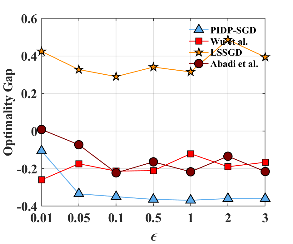
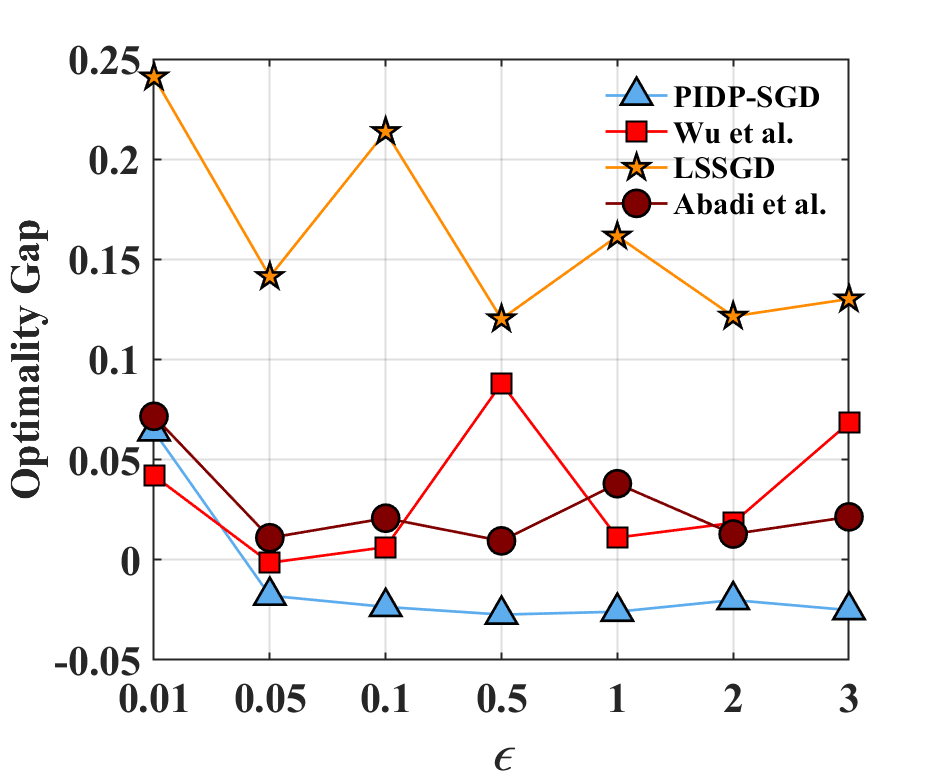
The time complexity of Algorithm 1 is 𝒪(Rnm2+RTlocalm)𝒪𝑅𝑛superscript𝑚2𝑅subscript𝑇𝑙𝑜𝑐𝑎𝑙𝑚\mathcal{O}\big{(}Rnm^{2}+RT_{local}m\big{)}. Under the case Tlocal=1subscript𝑇𝑙𝑜𝑐𝑎𝑙1T_{local}=1, it becomes 𝒪(Rnm2)𝒪𝑅𝑛superscript𝑚2\mathcal{O}\big{(}Rnm^{2}\big{)}, where R𝑅R is the total number of iterations. Fortunately, an efficient approach to calculate the Influence Function was given in [24], and the time complexity can be reduced to 𝒪(Rnm)𝒪𝑅𝑛𝑚\mathcal{O}\big{(}Rnm\big{)}. For some other previous performance improving method, the time complexity also increases, we show DP-LSSGD as an example here, whose time complexity is 𝒪(Rm2)𝒪𝑅superscript𝑚2\mathcal{O}\big{(}Rm^{2}\big{)}. Under the cases n>m𝑛𝑚n>m, our time complexity is larger than DP-LSSGD, and under high dimension cases, when nm𝑛𝑚n\leq m, our time complexity is better. However, both the theoretical and the experimental results of our method is much better than DP-LSSGD (shown in TABLE I and Figures 1 and  2). So under low dimension conditions, the sacrifice on time complexity is a trade-off against the model performance; and under high dimension conditions, our method is much better on both the model performance and the time complexity.

5.4 Privacy Guarantees

Theorem 5

In Algorithm 1, for δ1,δ2>0subscript𝛿1subscript𝛿20\delta_{1},\delta_{2}>0 and ϵ1,ϵ2>0subscriptitalic-ϵ1subscriptitalic-ϵ20\epsilon_{1},\epsilon_{2}>0, if (θ,z)𝜃𝑧\ell(\theta,z) is G𝐺G-Lipschitz over θ𝜃\theta, with

σcGTlog(1/δ1)nϵ1,σ(c)cGRlog(1.25R/δ2)nζϵ2,formulae-sequence𝜎𝑐𝐺𝑇1subscript𝛿1𝑛subscriptitalic-ϵ1subscript𝜎𝑐superscript𝑐𝐺𝑅1.25𝑅subscript𝛿2𝑛𝜁subscriptitalic-ϵ2\sigma\geq c\frac{G\sqrt{T\log(1/\delta_{1})}}{n\epsilon_{1}},\quad\sigma_{(c)}\geq c^{\prime}\frac{GR\sqrt{\log(1.25R/\delta_{2})}}{n\zeta\epsilon_{2}},

where T=TlocalR𝑇subscript𝑇𝑙𝑜𝑐𝑎𝑙𝑅T=T_{local}*R. It is (ϵ1+ϵ2,δ1+δ2subscriptitalic-ϵ1subscriptitalic-ϵ2subscript𝛿1subscript𝛿2\epsilon_{1}+\epsilon_{2},\delta_{1}+\delta_{2})-DP for some constants c,c𝑐superscript𝑐c,c^{\prime}.

Before the detailed proof, we first revisit the Gaussian mechanism.

Definition 7 (2subscript2\ell_{2}-sensitivity [15])

For DDsimilar-to𝐷superscript𝐷D\sim D^{\prime}, the 2subscript2\ell_{2}-sensitivity of a function f𝑓f is defined as:

S(f)=maxf(D)f(D)2.𝑆𝑓subscriptnorm𝑓𝐷𝑓superscript𝐷2S(f)=\max\|f(D)-f(D^{\prime})\|_{2}.

The 2subscript2\ell_{2}-sensitivity captures the magnitude by which a single individual’s data can change f𝑓f in the worst case.

Lemma 3

By Gaussian mechanism proposed in [15], (ϵitalic-ϵ\epsilon,δ𝛿\delta)-DP can be guaranteed if random noise b𝒩(0,σ2)similar-to𝑏𝒩0superscript𝜎2b\sim\mathcal{N}(0,\sigma^{2}) is added to a query, where σcS(f)ϵ𝜎𝑐𝑆𝑓italic-ϵ\sigma\geq c\frac{S(f)}{\epsilon} and c>2log(1.25/δ)𝑐21.25𝛿c>\sqrt{2\log(1.25/\delta)}.

Proof

We first analyze the privacy when computing the contributions ctsubscript𝑐𝑡c_{t} made by data instances.

Without privacy consideration, we have:

ct=θ~ztθr(g)=1n(Hθ~1θ(θr(g),zt)),subscript𝑐𝑡subscript~𝜃subscript𝑧𝑡subscriptsuperscript𝜃𝑔𝑟1𝑛superscriptsubscript𝐻~𝜃1subscript𝜃subscriptsuperscript𝜃𝑔𝑟subscript𝑧𝑡c_{t}=\widetilde{\theta}_{-z_{t}}-\theta^{(g)}_{r}=-\frac{1}{n}\left(-H_{\widetilde{\theta}}^{-1}\nabla_{\theta}\ell(\theta^{(g)}_{r},z_{t})\right),

where Hθ~=1ni=1nθ2(θ~,zi)subscript𝐻~𝜃1𝑛superscriptsubscript𝑖1𝑛superscriptsubscript𝜃2~𝜃subscript𝑧𝑖H_{\widetilde{\theta}}=\frac{1}{n}\sum_{i=1}^{n}\nabla_{\theta}^{2}\ell\left(\widetilde{\theta},z_{i}\right).

As a result, on adjacent databases, we have:

S(ct)𝑆subscript𝑐𝑡\displaystyle S(c_{t}) =ct(D)ct(D)2=1nHθ~1((θr(g),zt)(θr(g),zt))2.absentsubscriptnormsubscript𝑐𝑡𝐷subscript𝑐𝑡superscript𝐷21𝑛subscriptnormsuperscriptsubscript𝐻~𝜃1subscriptsuperscript𝜃𝑔𝑟subscript𝑧𝑡subscriptsuperscript𝜃𝑔𝑟superscriptsubscript𝑧𝑡2\displaystyle=\|c_{t}(D)-c_{t}(D^{\prime})\|_{2}=\frac{1}{n}\left\|H_{\widetilde{\theta}}^{-1}\left(\nabla\ell(\theta^{(g)}_{r},z_{t})-\nabla\ell(\theta^{(g)}_{r},z_{t}^{\prime})\right)\right\|_{2}.

If ()\ell(\cdot) is G𝐺G-Lipschitz over θ𝜃\theta, and Hθ~2ζsubscriptnormsubscript𝐻~𝜃2𝜁\left\|H_{\widetilde{\theta}}\right\|_{2}\geq\zeta, we have:

S(ct)2Gnζ.𝑆subscript𝑐𝑡2𝐺𝑛𝜁S(c_{t})\leq\frac{2G}{n\zeta}.

As shown in Algorithm 1, the contribution cztsubscript𝑐subscript𝑧𝑡c_{z_{t}} for data instance ztsubscript𝑧𝑡z_{t} is fixed during Tlocalsubscript𝑇𝑙𝑜𝑐𝑎𝑙T_{local} iterations and the fixed value only derives the privacy loss once. So the contribution made by ztsubscript𝑧𝑡z_{t} changes at most R𝑅R times during the whole T𝑇T iterations, and we only need to sum the privacy loss at most R𝑅R times.

Therefore, by Lemma 3, when computing ctsubscript𝑐𝑡c_{t}, if the added Gaussian random noise b(c)𝒩(0,σ2)similar-tosuperscript𝑏𝑐𝒩0superscript𝜎2b^{(c)}\sim\mathcal{N}\left(0,\sigma^{2}\right) satisfies:

σ>22log(1.25R/δ2)GRnζϵ2,𝜎221.25𝑅subscript𝛿2𝐺𝑅𝑛𝜁subscriptitalic-ϵ2\sigma>\frac{2\sqrt{2}\sqrt{\log(1.25R/\delta_{2})}GR}{n\zeta\epsilon_{2}},

(ϵ2Rsubscriptitalic-ϵ2𝑅\frac{\epsilon_{2}}{R}, δ2Rsubscript𝛿2𝑅\frac{\delta_{2}}{R})-DP at iteration t𝑡t is guaranteed by Gaussian mechanism. So, with c=2.83superscript𝑐2.83c^{\prime}=2.83, ctsubscript𝑐𝑡c_{t} calculation is (ϵ2subscriptitalic-ϵ2\epsilon_{2}, δ2subscript𝛿2\delta_{2})-DP overall.

Then, we consider the privacy which is naturally guaranteed. With the definition of DP (Definition 4), we have:

[𝒜(D)S]eϵ[𝒜(D)S]+δ.delimited-[]𝒜𝐷𝑆superscript𝑒italic-ϵdelimited-[]𝒜superscript𝐷𝑆𝛿\mathbb{P}\left[\mathcal{A}(D)\in S\right]\leq e^{\epsilon}\mathbb{P}\left[\mathcal{A}(D^{\prime})\in S\right]+\delta.

Via the discussion in [13], if all m𝑚m dimensions of model 𝒜(D)𝒜𝐷\mathcal{A}(D) are (ϵ,δitalic-ϵ𝛿\epsilon,\delta)-DP, then (ϵ,δitalic-ϵ𝛿\epsilon,\delta)-DP of 𝒜(D)𝒜𝐷\mathcal{A}(D) is guaranteed. So, in the following, we consider each dimension of 𝒜(D)𝒜𝐷\mathcal{A}(D).

(ϵ,δitalic-ϵ𝛿\epsilon,\delta)-DP naturally holds if the following inequality holds:

1δ[[𝒜(D)]iS]eϵ[[𝒜(D)]iS][[𝒜(D)]iS].1𝛿delimited-[]subscriptdelimited-[]𝒜𝐷𝑖𝑆superscript𝑒italic-ϵdelimited-[]subscriptdelimited-[]𝒜superscript𝐷𝑖𝑆delimited-[]subscriptdelimited-[]𝒜𝐷𝑖𝑆1-\frac{\delta}{\mathbb{P}\left[\left[\mathcal{A}(D)\right]_{i}\in S\right]}\leq e^{\epsilon}\frac{\mathbb{P}\left[\left[\mathcal{A}(D^{\prime})\right]_{i}\in S\right]}{\mathbb{P}\left[\left[\mathcal{A}(D)\right]_{i}\in S\right]}.

For simpicity, we set [[𝒜(D)]iS]=κδκ1delimited-[]subscriptdelimited-[]𝒜𝐷𝑖𝑆𝜅𝛿𝜅1\mathbb{P}\left[\left[\mathcal{A}(D)\right]_{i}\in S\right]=\frac{\kappa\delta}{\kappa-1} (κ>1𝜅1\kappa>1), then:

1κeϵ[[𝒜(D)]iS][[𝒜(D)]iS],1𝜅superscript𝑒italic-ϵdelimited-[]subscriptdelimited-[]𝒜superscript𝐷𝑖𝑆delimited-[]subscriptdelimited-[]𝒜𝐷𝑖𝑆\frac{1}{\kappa}\leq e^{\epsilon}\frac{\mathbb{P}\left[\left[\mathcal{A}(D^{\prime})\right]_{i}\in S\right]}{\mathbb{P}\left[\left[\mathcal{A}(D)\right]_{i}\in S\right]},

which can be written as:

ln([[𝒜(D)]iS][[𝒜(D)]iS])ϵ+ln(κ).delimited-[]subscriptdelimited-[]𝒜𝐷𝑖𝑆delimited-[]subscriptdelimited-[]𝒜superscript𝐷𝑖𝑆italic-ϵ𝜅\ln\left(\frac{\mathbb{P}\left[\left[\mathcal{A}(D)\right]_{i}\in S\right]}{\mathbb{P}\left[\left[\mathcal{A}(D^{\prime})\right]_{i}\in S\right]}\right)\leq\epsilon+\ln(\kappa). (15)

Considering that the model paramaters are uniformly distributed in a bounded parameter space, whose radius is r𝑟r, i.e., [𝒜(D)]i[r,r]subscriptdelimited-[]𝒜superscript𝐷𝑖𝑟𝑟\left[\mathcal{A}(D^{\prime})\right]_{i}\in[-r,r], and noting that 𝔼[𝒜(D)]=𝒜(D)𝔼delimited-[]𝒜superscript𝐷𝒜𝐷\mathbb{E}\left[\mathcal{A}(D^{\prime})\right]=\mathcal{A}(D), where the expectation is taken over the single different z𝑧z between D𝐷D and Dsuperscript𝐷D^{\prime}, then [[𝒜(D)]iS]delimited-[]subscriptdelimited-[]𝒜𝐷𝑖𝑆\mathbb{P}\left[\left[\mathcal{A}(D)\right]_{i}\in S\right] is located in [rκδ(κ1),rκδ(κ1)]𝑟𝜅𝛿𝜅1𝑟𝜅𝛿𝜅1\big{[}\frac{-r\kappa\delta}{(\kappa-1)},\frac{r\kappa\delta}{(\kappa-1)}\big{]}.

With the largest fluctuation ctsubscript𝑐𝑡c_{t}, then for the ithsuperscript𝑖𝑡i^{th} element of 𝒜(D)𝒜𝐷\mathcal{A}(D) and 𝒜(D)𝒜superscript𝐷\mathcal{A}(D^{\prime}),

[𝒜(D)𝒜(D)]i=[𝒜(D)]i[𝒜(D)]i[ct]i,subscriptdelimited-[]𝒜superscript𝐷𝒜𝐷𝑖subscriptdelimited-[]𝒜superscript𝐷𝑖subscriptdelimited-[]𝒜𝐷𝑖subscriptdelimited-[]subscript𝑐𝑡𝑖\left[\mathcal{A}(D^{\prime})-\mathcal{A}(D)\right]_{i}=\left[\mathcal{A}(D^{\prime})\right]_{i}-\left[\mathcal{A}(D)\right]_{i}\leq\left[c_{t}\right]_{i},

where []isubscriptdelimited-[]𝑖[\cdot]_{i} represents the ithsuperscript𝑖𝑡i^{th} element of a vector.

As a result, if [ct]i0subscriptdelimited-[]subscript𝑐𝑡𝑖0\left[c_{t}\right]_{i}\geq 0, then [[ct]irκδ(κ1),rκδ(κ1)]subscriptdelimited-[]subscript𝑐𝑡𝑖𝑟𝜅𝛿𝜅1𝑟𝜅𝛿𝜅1\big{[}[c_{t}]_{i}-\frac{r\kappa\delta}{(\kappa-1)},\frac{r\kappa\delta}{(\kappa-1)}\big{]} is the area that [[𝒜(D)]iS]delimited-[]subscriptdelimited-[]𝒜superscript𝐷𝑖𝑆\mathbb{P}\left[\left[\mathcal{A}(D^{\prime})\right]_{i}\in S\right]; otherwise, [rκδ(κ1),[ct]i+rκδ(κ1)]𝑟𝜅𝛿𝜅1subscriptdelimited-[]subscript𝑐𝑡𝑖𝑟𝜅𝛿𝜅1\big{[}\frac{-r\kappa\delta}{(\kappa-1)},[c_{t}]_{i}+\frac{r\kappa\delta}{(\kappa-1)}\big{]} is the area that [[𝒜(D)]iS]delimited-[]subscriptdelimited-[]𝒜superscript𝐷𝑖𝑆\mathbb{P}\left[\left[\mathcal{A}(D^{\prime})\right]_{i}\in S\right].

Thus, we have:

[[𝒜(D)]iS]{κδ(κ1)[ct]i2r,[ct]i0,κδ(κ1)+[ct]i2r,[ct]i<0.\mathbb{P}\left[\left[\mathcal{A}(D^{\prime})\right]_{i}\in S\right]\leq\left\{\begin{aligned} &\frac{\kappa\delta}{(\kappa-1)}-\frac{\left[c_{t}\right]_{i}}{2r},\quad\left[c_{t}\right]_{i}\geq 0,\\ &\frac{\kappa\delta}{(\kappa-1)}+\frac{\left[c_{t}\right]_{i}}{2r},\quad\left[c_{t}\right]_{i}<0.\end{aligned}\right.

If |[ct]i|2rκδ(κ1)subscriptdelimited-[]subscript𝑐𝑡𝑖2𝑟𝜅𝛿𝜅1|[c_{t}]_{i}|\geq\frac{2r\kappa\delta}{(\kappa-1)}, then [[𝒜(D)]iS[𝒜(D)]iS]=0delimited-[]subscriptdelimited-[]𝒜𝐷𝑖𝑆subscriptdelimited-[]𝒜superscript𝐷𝑖𝑆0\mathbb{P}\left[\left[\mathcal{A}(D)\right]_{i}\in S\cap\left[\mathcal{A}(D^{\prime})\right]_{i}\in S\right]=0 so ztsubscript𝑧𝑡z_{t} has significant contribution, we directly jump to line 13 as shown in Algorithm 1. If |[ct]i|<2rκδ(κ1)subscriptdelimited-[]subscript𝑐𝑡𝑖2𝑟𝜅𝛿𝜅1|[c_{t}]_{i}|<\frac{2r\kappa\delta}{(\kappa-1)} for all i𝑖i, then by (15), (ϵ1,δ1subscriptitalic-ϵ1subscript𝛿1\epsilon_{1},\delta_{1})-DP is guaranteed if for all m𝑚m dimensions, the following inequality holds:

ln(2rκδ12rκδ1(κ1)sign([ct]i)[ct]i)ϵ1+ln(κ),2𝑟𝜅subscript𝛿12𝑟𝜅subscript𝛿1𝜅1𝑠𝑖𝑔𝑛subscriptdelimited-[]subscript𝑐𝑡𝑖subscriptdelimited-[]subscript𝑐𝑡𝑖subscriptitalic-ϵ1𝜅\ln\left(\frac{2r\kappa\delta_{1}}{2r\kappa\delta_{1}-(\kappa-1)sign(\left[c_{t}\right]_{i})\left[c_{t}\right]_{i}}\right)\leq\epsilon_{1}+\ln(\kappa),

where sign()𝑠𝑖𝑔𝑛sign(\cdot) is the signum function and 1im1𝑖𝑚1\leq i\leq m.

We set κ=eϵ1𝜅superscript𝑒subscriptitalic-ϵ1\kappa=e^{\epsilon_{1}}, then via Algorithm 1, (ϵ1,δ1subscriptitalic-ϵ1subscript𝛿1\epsilon_{1},\delta_{1})-DP is naturally guaranteed in lines 10 and 11.

Finally, we consider the privacy when training the model.

For the data instances whose contributions are not so much, (ϵ1,δ1)subscriptitalic-ϵ1subscript𝛿1(\epsilon_{1},\delta_{1})-DP is naturally guaranteed, as analyzed above. And if the contribution is large, via moments accountant method, if b𝒩(0,σ2Im)similar-to𝑏𝒩0superscript𝜎2subscript𝐼𝑚b\sim\mathcal{N}\big{(}0,\sigma^{2}I_{m}\big{)} and σ=𝒪(GTlog(1/δ1)nϵ1)𝜎𝒪𝐺𝑇1subscript𝛿1𝑛subscriptitalic-ϵ1\sigma=\mathcal{O}\big{(}\frac{G\sqrt{T\log(1/\delta_{1})}}{n\epsilon_{1}}\big{)}, then (ϵ1,δ1subscriptitalic-ϵ1subscript𝛿1\epsilon_{1},\delta_{1})-DP can be guaranteed when training.

Then, by composition theorems [15], Algorithm 1 is (ϵ1+ϵ2subscriptitalic-ϵ1subscriptitalic-ϵ2\epsilon_{1}+\epsilon_{2}, δ1+δ2subscript𝛿1subscript𝛿2\delta_{1}+\delta_{2})-DP overall, which completes the proof.

Theorem 5 shows that the privacy of Algorithm 1 consists of two parts: (1) computing the contribution ctsubscript𝑐𝑡c_{t} and (2) training the model by DP-SGD. Specifically, ϵ1,δ1subscriptitalic-ϵ1subscript𝛿1\epsilon_{1},\delta_{1} (σ𝜎\sigma) are for the privacy when training the model and ϵ2,δ2subscriptitalic-ϵ2subscript𝛿2\epsilon_{2},\delta_{2} (σ(c)subscript𝜎𝑐\sigma_{(c)}) are for the privacy when computing ctsubscript𝑐𝑡c_{t}.

Remark 9

In the proof, we analyze the DP of the SGD process by the moments accountant method and for DP of computing ctsubscript𝑐𝑡c_{t}, the analysis is based on the 2subscript2\ell_{2}-sensitivity and Gaussian mechanism. The reason is that for SGD, tracking the privacy loss during T𝑇T iterations is an important part and the moments accountant method naturally solves the problem. However, computing ctsubscript𝑐𝑡c_{t} is only for the decision process and during Tlocalsubscript𝑇𝑙𝑜𝑐𝑎𝑙T_{local} iterations, cztsubscript𝑐subscript𝑧𝑡c_{z_{t}} for a certain data instance ztsubscript𝑧𝑡z_{t} is fixed and only calculated once, so it derives corresponding privacy loss only once. Thus, there is no need to track the privacy loss over the whole training iterations. As a result, we discuss the privacy leakage brought by ctsubscript𝑐𝑡c_{t} from the point of view: 2subscript2\ell_{2}-sensitivity and Gaussian mechanism.

In Algorithm 1, noise is only added when training with a partition of data instances, which leads better excess risk bounds. In the following, we suppose that there are k𝑘k data instances affect the model significantly and measure the improvement brought by our proposed ‘Performance Improving’ algorithm.

Table 1: Comparisons on excess risk bounds between our method and other methods.
G𝐺G L𝐿L S.C. C PL EPR
[4] \checkmark \checkmark ×\times \checkmark ×\times 𝒪(mnϵ+1n)𝒪𝑚𝑛italic-ϵ1𝑛\mathcal{O}\left(\frac{\sqrt{m}}{n\epsilon}+\frac{1}{\sqrt{n}}\right)
[16] \checkmark ×\times \checkmark \checkmark ×\times 𝒪(mn2ϵ2+1n)𝒪𝑚superscript𝑛2superscriptitalic-ϵ21𝑛\mathcal{O}\left(\frac{m}{n^{2}\epsilon^{2}}+\frac{1}{n}\right)
[16] \checkmark ×\times ×\times \checkmark ×\times 𝒪(mnϵ+1n)𝒪𝑚𝑛italic-ϵ1𝑛\mathcal{O}\left(\frac{\sqrt{m}}{n\epsilon}+\frac{1}{\sqrt{n}}\right)
Ours \checkmark \checkmark ×\times ×\times \checkmark 𝒪(min{mn2ϵ2+1n,mn1.5ϵ+m1.5n2.5ϵ3})𝒪𝑚superscript𝑛2superscriptitalic-ϵ21𝑛𝑚superscript𝑛1.5italic-ϵsuperscript𝑚1.5superscript𝑛2.5superscriptitalic-ϵ3\mathcal{O}\left(\min\left\{\frac{m}{n^{2}\epsilon^{2}}+\frac{1}{n},\frac{\sqrt{m}}{n^{1.5}\epsilon}+\frac{m^{1.5}}{n^{2.5}\epsilon^{3}}\right\}\right)
Ours (PIDP-SGD) \checkmark \checkmark ×\times ×\times \checkmark 𝒪(min{kmn3ϵ2+1n,kmn2.5ϵ2+1n1.5,(km)1.5n2ϵ3+ϵkmn})𝒪𝑘𝑚superscript𝑛3superscriptitalic-ϵ21𝑛𝑘𝑚superscript𝑛2.5superscriptitalic-ϵ21superscript𝑛1.5superscript𝑘𝑚1.5superscript𝑛2superscriptitalic-ϵ3italic-ϵ𝑘𝑚𝑛\mathcal{O}\left(\min\left\{\frac{km}{n^{3}\epsilon^{2}}+\frac{1}{n},\frac{km}{n^{2.5}\epsilon^{2}}+\frac{1}{n^{1.5}},\frac{(km)^{1.5}}{n^{2}\epsilon^{3}}+\frac{\epsilon}{\sqrt{km}n}\right\}\right)
  • 1

    k𝑘k is the number of data instances that affect the model significantly, mentioned above.

5.5 Utility Analysis

5.5.1 Excess Empirical Risk

Theorem 6

Suppose that (θ,z)𝜃𝑧\ell(\theta,z) is G𝐺G-Lipschitz, L𝐿L-smooth, and satisfies PL condition over θ𝜃\theta. With learning rate α=1L𝛼1𝐿\alpha=\frac{1}{L} and k𝑘k data instances affect the model significantly, the excess empirical risk bound can be improved to:

𝔼[L(θpriv;D)L]𝒪(kmG2log(1/δ1)log(n)n3ϵ12),𝔼delimited-[]𝐿subscript𝜃𝑝𝑟𝑖𝑣𝐷superscript𝐿𝒪𝑘𝑚superscript𝐺21subscript𝛿1𝑛superscript𝑛3superscriptsubscriptitalic-ϵ12\mathbb{E}\left[L(\theta_{priv};D)-L^{*}\right]\leq\mathcal{O}\left(\frac{kmG^{2}\log(1/\delta_{1})\log(n)}{n^{3}\epsilon_{1}^{2}}\right),

where the expectation is taken over the algorithm and dataset D𝐷D, T=𝒪(log(n))𝑇𝒪𝑛T=\mathcal{O}(\log(n)).

Proof

As in the proof of Theorem 1, if there are k𝑘k data instances affect the model significantly, (4) can be written as:

𝔼[L(θt+1;D)L(θt;D)]𝔼delimited-[]𝐿subscript𝜃𝑡1𝐷𝐿subscript𝜃𝑡𝐷\displaystyle\mathbb{E}\left[L(\theta_{t+1};D)-L(\theta_{t};D)\right] (L)𝔼[θL(θt;D),θt+1θt+L2θt+1θt22]𝐿𝔼delimited-[]subscript𝜃𝐿subscript𝜃𝑡𝐷subscript𝜃𝑡1subscript𝜃𝑡𝐿2superscriptsubscriptnormsubscript𝜃𝑡1subscript𝜃𝑡22\displaystyle\overset{(L)}{\leq}\mathbb{E}\left[\left<\nabla_{\theta}L(\theta_{t};D),\theta_{t+1}-\theta_{t}\right>+\frac{L}{2}\|\theta_{t+1}-\theta_{t}\|_{2}^{2}\right]
12L𝔼D[θL(θt;D)22]+kn12L𝔼b22,absent12𝐿subscript𝔼𝐷delimited-[]superscriptsubscriptnormsubscript𝜃𝐿subscript𝜃𝑡𝐷22𝑘𝑛12𝐿𝔼superscriptsubscriptnorm𝑏22\displaystyle\leq-\frac{1}{2L}\mathbb{E}_{D}\left[\|\nabla_{\theta}L(\theta_{t};D)\|_{2}^{2}\right]+\frac{k}{n}\frac{1}{2L}\mathbb{E}\|b\|_{2}^{2},

where the last inequality holds because we have the probability kn𝑘𝑛\frac{k}{n} to reach the data instance ztsubscript𝑧𝑡z_{t} ‘meeting’ the noise.

Thus, we have:

𝔼[L(θt+1;D)L(θt;D)]𝔼delimited-[]𝐿subscript𝜃𝑡1𝐷𝐿subscript𝜃𝑡𝐷\displaystyle\mathbb{E}\left[L(\theta_{t+1};D)-L(\theta_{t};D)\right] μL(𝔼D[L(θt;D)L])+knmσ22L.absent𝜇𝐿subscript𝔼𝐷delimited-[]𝐿subscript𝜃𝑡𝐷superscript𝐿𝑘𝑛𝑚superscript𝜎22𝐿\displaystyle\leq-\frac{\mu}{L}(\mathbb{E}_{D}\left[L(\theta_{t};D)-L^{*}\right])+\frac{k}{n}\frac{m\sigma^{2}}{2L}.

Then, summing over T𝑇T iterations, we have:

𝔼[L(θT;D)L]𝔼delimited-[]𝐿subscript𝜃𝑇𝐷superscript𝐿\displaystyle\mathbb{E}[L(\theta_{T};D)-L^{*}] (1μL)T(𝔼D[L(θ0;D)L])+kmσ22Ln(i=0T1(1μL)i)absentsuperscript1𝜇𝐿𝑇subscript𝔼𝐷delimited-[]𝐿subscript𝜃0𝐷superscript𝐿𝑘𝑚superscript𝜎22𝐿𝑛superscriptsubscript𝑖0𝑇1superscript1𝜇𝐿𝑖\displaystyle\leq(1-\frac{\mu}{L})^{T}(\mathbb{E}_{D}\left[L(\theta_{0};D)-L^{*}\right])+\frac{km\sigma^{2}}{2Ln}\left(\sum_{i=0}^{T-1}(1-\frac{\mu}{L})^{i}\right)
(1μL)T(𝔼D[L(θ0;D)L])+kmσ22μn.absentsuperscript1𝜇𝐿𝑇subscript𝔼𝐷delimited-[]𝐿subscript𝜃0𝐷superscript𝐿𝑘𝑚superscript𝜎22𝜇𝑛\displaystyle\leq(1-\frac{\mu}{L})^{T}(\mathbb{E}_{D}\left[L(\theta_{0};D)-L^{*}\right])+\frac{km\sigma^{2}}{2\mu n}.

Taking T=𝒪(log(n3ϵ12kmG2))𝑇𝒪superscript𝑛3superscriptsubscriptitalic-ϵ12𝑘𝑚superscript𝐺2T=\mathcal{O}\left(\log\left(\frac{n^{3}\epsilon_{1}^{2}}{kmG^{2}}\right)\right) and σ𝜎\sigma discussed before:

𝔼[L(θpriv;D)L]𝔼delimited-[]𝐿subscript𝜃𝑝𝑟𝑖𝑣𝐷superscript𝐿\displaystyle\mathbb{E}[L(\theta_{priv};D)-L^{*}] =𝔼[L(θT;D)L]O(kmG2log(1/δ1)log(n)n3ϵ12),absent𝔼delimited-[]𝐿subscript𝜃𝑇𝐷superscript𝐿𝑂𝑘𝑚superscript𝐺21subscript𝛿1𝑛superscript𝑛3superscriptsubscriptitalic-ϵ12\displaystyle=\mathbb{E}[L(\theta_{T};D)-L^{*}]\leq O\left(\frac{kmG^{2}\log(1/\delta_{1})\log(n)}{n^{3}\epsilon_{1}^{2}}\right),

where the expectation is taken over D𝐷D and the algorithm.

Noting that kn<1𝑘𝑛1\frac{k}{n}<1, we have:

𝒪(kmG2log(1/δ)log(n)n3ϵ2)<𝒪(mG2log(1/δ)log(n)n2ϵ2).𝒪𝑘𝑚superscript𝐺21𝛿𝑛superscript𝑛3superscriptitalic-ϵ2𝒪𝑚superscript𝐺21𝛿𝑛superscript𝑛2superscriptitalic-ϵ2\mathcal{O}\left(\frac{kmG^{2}\log(1/\delta)\log(n)}{n^{3}\epsilon^{2}}\right)<\mathcal{O}\left(\frac{mG^{2}\log(1/\delta)\log(n)}{n^{2}\epsilon^{2}}\right).

As a result, the excess empirical risk bound brought by Theorem 6 is better than Theorem 1.

5.5.2 Excess Population Risk

Like in Section IV, we first analyze the generalization error. Via the proof of Theorem 2, we find that the generalization error is only related to θiTθT2subscriptnormsuperscriptsubscript𝜃𝑖𝑇superscript𝜃𝑇2\|\theta_{i}^{T}-\theta^{T}\|_{2} and L(θpriv;D)𝐿subscript𝜃𝑝𝑟𝑖𝑣𝐷L(\theta_{priv};D), and these terms are only determined by the optimization process, so the generalization error of Algorithm 1 is the same as which given in Theorem 2. Then we come to the excess population risk.

Theorem 7

If ()\ell(\cdot) is G𝐺G-Lipschitz, L𝐿L-smooth, and satisfies the PL condition over θ𝜃\theta. With learning rate α=1L𝛼1𝐿\alpha=\frac{1}{L}, T=𝒪(log(n))𝑇𝒪𝑛T=\mathcal{O}(\log(n)) and k𝑘k data instances affect the model significantly, the excess population risk can be improved to:

𝔼[L𝒫(θpriv)minθL𝒫(θ)]𝔼delimited-[]subscript𝐿𝒫subscript𝜃𝑝𝑟𝑖𝑣subscript𝜃subscript𝐿𝒫𝜃\displaystyle\mathbb{E}\left[L_{\mathcal{P}}\left(\theta_{priv}\right)-\min_{\theta}L_{\mathcal{P}}\left(\theta\right)\right]
𝒪(min{kmn3ϵ2+1n,kmn2.5ϵ2+1n1.5,(km)1.5n2ϵ3+ϵkmn}).absent𝒪𝑘𝑚superscript𝑛3superscriptitalic-ϵ21𝑛𝑘𝑚superscript𝑛2.5superscriptitalic-ϵ21superscript𝑛1.5superscript𝑘𝑚1.5superscript𝑛2superscriptitalic-ϵ3italic-ϵ𝑘𝑚𝑛\displaystyle\leq\mathcal{O}\left(\min\left\{\frac{km}{n^{3}\epsilon^{2}}+\frac{1}{n},\frac{km}{n^{2.5}\epsilon^{2}}+\frac{1}{n^{1.5}},\frac{(km)^{1.5}}{n^{2}\epsilon^{3}}+\frac{\epsilon}{\sqrt{km}n}\right\}\right).

The proof is similar to Theorem 3 and the discussion given in Remark 4. The first, second, third and last terms on the right side of the inequality are derived from taking τ=𝒪(1),𝒪(n)𝜏𝒪1𝒪𝑛\tau=\mathcal{O}(1),\mathcal{O}(\sqrt{n}) and 𝒪(nϵ/km)𝒪𝑛italic-ϵ𝑘𝑚\mathcal{O}(n\epsilon/\sqrt{km}), respectively.

Noting that kn<1𝑘𝑛1\frac{k}{n}<1, the result is better than which given by Theorem 3.

Remark 10

Note that ϵitalic-ϵ\epsilon and ϵ1subscriptitalic-ϵ1\epsilon_{1} can be set almost the same, so we do not distinguish them in the discussion above.

For the first time, we theoretically prove that the excess risk of differential privacy models can be better by considering data heterogeneity. It may give new inspirations to the utility analysis in the future work.

6 Comparison with Related Work

6.1 Utility Bounds

For excess empirical risk, by detailed theoretical analysis, we give a sharper bound for DP-SGD. Our analyzed excess empirical risk bound of is better than which proposed by [5, 44, 40, 4] and achieves the best result 𝒪(mn2ϵ2)𝒪𝑚superscript𝑛2superscriptitalic-ϵ2\mathcal{O}\big{(}\frac{m}{n^{2}\epsilon^{2}}\big{)}. For our proposed ‘performance improving’ method: PIDP-SGD, our analyzed excess empirical risk bound is further tighter by a factor of 𝒪(kn)𝒪𝑘𝑛\mathcal{O}\big{(}\frac{k}{n}\big{)}. It is worth emphasizing that most of the methods proposed previously assume that the loss function is convex, which is not required in our method. Under this circumstance, we achieve a better result, which is attractive. Additionally, for the non-convex analysis given in [43], the excess empirical risk bound of our analyzed DP-SGD method is better by a factor of 𝒪(log(n))𝒪𝑛\mathcal{O}\big{(}\log(n)\big{)} (as discussed in Remark 3) and the PIDP-SGD method is better by a factor of 𝒪(klog(n)n)𝒪𝑘𝑛𝑛\mathcal{O}\big{(}\frac{k\log(n)}{n}\big{)}. Details can be found in Table 1, in which G,L𝐺𝐿G,L, S.C., C, PL represent G𝐺G-Lipschitz, L𝐿L-smooth, strongly convex, convex and PL inequality, respectively and EER, EPR denote the Excess Empirical Risk and the Empirical Population Risk, respectively.

Previous works always discuss the excess empirical risk but seldom analyze the excess population risk, here we compare our method with the best result 𝒪(mn2ϵ2+1n)𝒪𝑚superscript𝑛2superscriptitalic-ϵ21𝑛\mathcal{O}\big{(}\frac{m}{n^{2}\epsilon^{2}}+\frac{1}{n}\big{)} given in [16], under strongly convex condition. As shown in Table I, our result is better by a factor up to 𝒪(1n)𝒪1𝑛\mathcal{O}\big{(}\frac{1}{\sqrt{n}}\big{)} under the best case. When it comes to our proposed PIDP-SGD method, our result is further improved by a factor up to 𝒪(kn)𝒪𝑘𝑛\mathcal{O}\big{(}\frac{k}{n}\big{)}. Noting that the best result given in [16] requires the loss function to be strongly convex, which means that our result is not only better but also strictly more general than which given in [16]. For the result under the convex assumption 𝒪(mnϵ+1n)𝒪𝑚𝑛italic-ϵ1𝑛\mathcal{O}\big{(}\frac{\sqrt{m}}{n\epsilon}+\frac{1}{\sqrt{n}}\big{)}, our results (both the original one and the one given by PIDP-SGD) are much better. Although it is hard to compare the convexity and the PL condition, our results can be applied to some of the non-convex models (as shown in Definition 5).
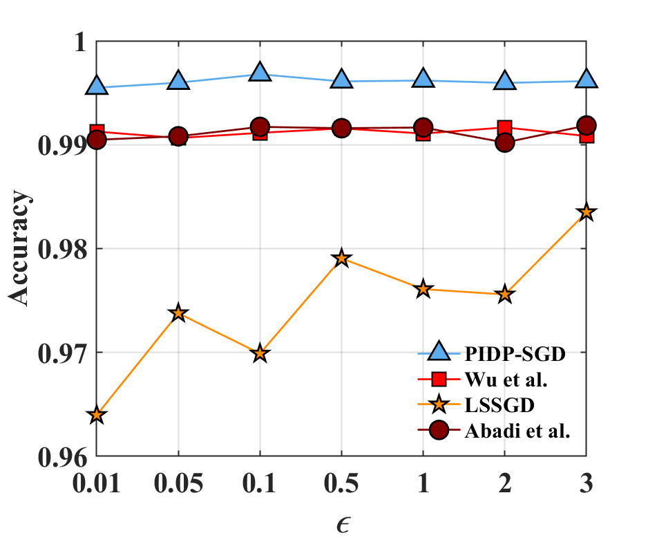
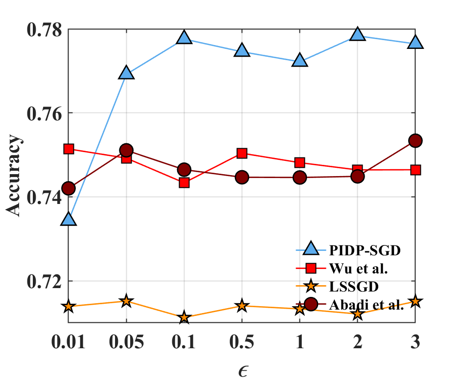
Refer to caption
(a) KDDCup99 (LR)
Refer to caption
(b) Adult (LR)
Refer to caption
(c) Bank (LR)
Refer to caption
(d) KDDCup99 (MLP)
Refer to caption
(e) Adult (MLP)
Refer to caption
(f) Bank (MLP)
Figure 1: Accuracy over ϵitalic-ϵ\epsilon, LR denotes logistic regression model and MLP denotes the deep learning model.
Refer to caption
(a) KDDCup99 (LR)
Refer to caption
(b) Adult (LR)
Refer to caption
(c) Bank (LR)
Refer to caption
(d) KDDCup99 (MLP)
Refer to caption
(e) Adult (MLP)
Refer to caption
(f) Bank (MLP)
Figure 2: Optimality gap over ϵitalic-ϵ\epsilon, LR denotes logistic regression model and MLP denotes the deep learning model.

7 Experimental Results

Experiments on several real datasets are performed on the classification task. Since our method is based on SGD, we compare our method with previous DP-SGD methods. Specifically, we compare our method with the gradient perturbation method proposed in [1], the output perturbation method proposed in [44] and the DP-LSSGD method proposed in [39]. The performance is measured in terms of classification accuracy and the optimality gap. The accuracy represents the performance on the testing set, and the optimality gap represents the excess empirical risk on the training set. The optimality gap is denoted by L(θpriv;D)L𝐿subscript𝜃𝑝𝑟𝑖𝑣𝐷superscript𝐿L(\theta_{priv};D)-L^{*}.

We use both logistic regression model and deep learning model on the datasets KDDCup99 [20], Adult [12] and Bank [31], where the total number of data instances are 70000, 45222, and 41188, respectively. In the experiments, to make the model satisfies the assumptions (such as PL condition) mentioned in the theoretical part, the deep learning model is denoted by Multi-layer Perceptron (MLP) with one hidden layer whose size is the same as the input layer. Training and testing datasets are chosen randomly.

In all the experiments, total iteration rounds T𝑇T is chosen by cross-validation. For our performance improving method, we set RTlocal=T𝑅subscript𝑇𝑙𝑜𝑐𝑎𝑙𝑇RT_{local}=T. We evaluate the performance of our proposed PIDP-SGD method and some of previous algorithms over the differential privacy budget ϵitalic-ϵ\epsilon. For ϵitalic-ϵ\epsilon, we set it from 0.01 to 3, and in the PIDP-SGD method, we set ϵ1=3ϵ2=3ϵ/4subscriptitalic-ϵ13subscriptitalic-ϵ23italic-ϵ4\epsilon_{1}=3\epsilon_{2}=3\epsilon/4 to guarantee ϵ1+ϵ2=ϵsubscriptitalic-ϵ1subscriptitalic-ϵ2italic-ϵ\epsilon_{1}+\epsilon_{2}=\epsilon. The results are shown in Figure 1 and Figure 2.

Figure 1 shows that as the privacy budget ϵitalic-ϵ\epsilon increases, so does the accuracy, which follows the intuition. When applying the PIDP-SGD algorithm, the accuracy rises on most datasets, which means that our proposed ‘performance improving’ method is effective. Meanwhile, when ϵitalic-ϵ\epsilon is small, the difference (on accuracy) between traditional methods and ‘performance improving’ method is also small. However, as ϵitalic-ϵ\epsilon increases, the ‘performance improving’ method becomes more and more competitive. The reason is that larger ϵitalic-ϵ\epsilon means that more data instances ‘escape’ the injected noise, leading to better accuracies.

Figure 2 shows that on some datasets, by applying PIDP-SGD algorithm, the optimality gap of our method is almost 0, which means that it achieves almost the same performance as the model without privacy in some scenarios. Besides, similar to the accuracy in Figure 1, the optimality gap decreases as ϵitalic-ϵ\epsilon increases, which follows our intuition. Moreover, on some datasets, the performance of some of the methods fluctuates. The reason is that in the setting of differential privacy, random noise is injected into the model, so it is a common phenomenon.

Additionally, on some datasets, the performance of our ‘performance improving’ method is worse when ϵitalic-ϵ\epsilon is small, the reason is that part of the privacy budget is allocated to ctsubscript𝑐𝑡c_{t} (in our experiments, we set ϵ1=3ϵ2=3ϵ/4subscriptitalic-ϵ13subscriptitalic-ϵ23italic-ϵ4\epsilon_{1}=3\epsilon_{2}=3\epsilon/4, so the ratio is 1/4141/4), which means ‘pure privacy budget’ on the model is smaller. Thus, with the increase of ϵitalic-ϵ\epsilon, the ‘performance improving’ method becomes more competitive, which has been analyzed before in Section V.C𝐶C. Experimental results show that our proposed PIDP-SGD algorithm significantly improves the performance under most circumstances.

8 Conclusions

In this paper, we give sharper excess risk bounds of traditional DP-SGD paradigm, including the excess empirical risk bound and the excess population risk bound. Theoretical results show that our given excess risk bounds achieve better excess risk bounds than some of the best previous methods under non-convex condition, and even better than previous results under convex condition. Meanwhile, based on DP-SGD, we attempt to improve the performance from a new perspective: considering data heterogeneity, rather than treating all data the same. In particular, we introduce the influence function (IF) to DP-SGD to analyze the contribution of each data instance to the final model, and the approximation error analysis shows that IF is reasonable to approximate the contribution. In this way, we propose the PIDP-SGD algorithm: only adding noise to the data demonstrating significant contributions (more than eϵsuperscript𝑒italic-ϵe^{\epsilon}) when training. Detailed theoretical analysis and experimental results show that our proposed ‘Performance Improving’ algorithm achieves better performance, without the convex assumption. Moreover, the new perspective from the view of treating different data instances differently may give new inspirations to future work, including the privacy analysis and the utility analysis.

References

  • [1] Abadi, M., Chu, A., Goodfellow, I., McMahan, H.B., Mironov, I., Talwar, K., Zhang, L.: Deep learning with differential privacy. In: Proceedings of the 2016 ACM SIGSAC Conference on Computer and Communications Security. pp. 308–318 (2016)
  • [2] Arora, R., Upadhyay, J.: On differentially private graph sparsification and applications. In: Advances in Neural Information Processing Systems. pp. 13378–13389 (2019)
  • [3] Backes, M., Berrang, P., Humbert, M., Manoharan, P.: Membership privacy in microrna-based studies. In: Proceedings of the 2016 ACM SIGSAC Conference on Computer and Communications Security. p. 319–330 (2016)
  • [4] Bassily, R., Feldman, V., Talwar, K., Guha Thakurta, A.: Private stochastic convex optimization with optimal rates. In: Advances in Neural Information Processing Systems. pp. 11279–11288 (2019)
  • [5] Bassily, R., Smith, A., Thakurta, A.: Private empirical risk minimization: Efficient algorithms and tight error bounds. In: 2014 IEEE 55th Annual Symposium on Foundations of Computer Science. pp. 464–473 (2014)
  • [6] Bernstein, G., Sheldon, D.R.: Differentially private bayesian linear regression. In: Advances in Neural Information Processing Systems. pp. 523–533 (2019)
  • [7] Carlini, N., Liu, C., Erlingsson, U., Kos, J., Song, D.: The secret sharer: Evaluating and testing unintended memorization in neural networks. In: Proceedings of the 28th USENIX Conference on Security Symposium. p. 267–284 (2019)
  • [8] Charles, Z., Papailiopoulos, D.: Stability and generalization of learning algorithms that converge to global optima. In: Proceedings of the 35th International Conference on Machine Learning. pp. 745–754 (2018)
  • [9] Chaudhuri, K., Monteleoni, C., Sarwate, A.D.: Differentially private empirical risk minimization. Journal of Machine Learning Research pp. 1069–1109 (2011)
  • [10] Chen, Z., Ni, T., Zhong, H., Zhang, S., Cui, J.: Differentially private double spectrum auction with approximate social welfare maximization. IEEE Transactions on Information Forensics and Security pp. 2805–2818 (2019)
  • [11] Csiba, D., Richtárik, P.: Global convergence of arbitrary-block gradient methods for generalized polyak-łojasiewicz functions. arXiv preprint arXiv:1709.03014 (2017)
  • [12] Dua, D., Graff, C.: UCI machine learning repository (2017)
  • [13] Dwork, C.: Differential privacy. In: International Colloquium on Automata, Languages, and Programming. pp. 1–12 (2006)
  • [14] Dwork, C., McSherry, F., Nissim, K., Smith, A.: Calibrating noise to sensitivity in private data analysis. In: Theory of cryptography conference. pp. 265–284 (2006)
  • [15] Dwork, C., Roth, A., et al.: The algorithmic foundations of differential privacy. Foundations and Trends® in Theoretical Computer Science pp. 211–407 (2014)
  • [16] Feldman, V., Koren, T., Talwar, K.: Private stochastic convex optimization: Optimal rates in linear time. In: Proceedings of the 52nd Annual ACM SIGACT Symposium on Theory of Computing. p. 439–449 (2020)
  • [17] Fredrikson, M., Lantz, E., Jha, S., Lin, S., Page, D., Ristenpart, T.: Privacy in pharmacogenetics: An end-to-end case study of personalized warfarin dosing. In: 23rd {{\{USENIX}}\} Security Symposium ({{\{USENIX}}\} Security 14). pp. 17–32 (2014)
  • [18] Hardt, M., Recht, B., Singer, Y.: Train faster, generalize better: Stability of stochastic gradient descent. In: International Conference on Machine Learning. pp. 1225–1234 (2016)
  • [19] Heikkilä, M., Jälkö, J., Dikmen, O., Honkela, A.: Differentially private markov chain monte carlo. In: Advances in Neural Information Processing Systems 32, pp. 4115–4125 (2019)
  • [20] Hettich, S., Bay, S.D.: The uci kdd archive (1999)
  • [21] Jayaraman, B., Evans, D.: Evaluating differentially private machine learning in practice. In: Proceedings of the 28th USENIX Conference on Security Symposium. pp. 1895–1912 (2019)
  • [22] Karimi, H., Nutini, J., Schmidt, M.: Linear convergence of gradient and proximal-gradient methods under the polyak-łojasiewicz condition. In: Joint European Conference on Machine Learning and Knowledge Discovery in Databases. pp. 795–811 (2016)
  • [23] Kifer, D., Smith, A., Thakurta, A.: Private convex empirical risk minimization and high-dimensional regression. In: Conference on Learning Theory. pp. 25–1 (2012)
  • [24] Koh, P.W., Liang, P.: Understanding black-box predictions via influence functions. In: Proceedings of the 34th International Conference on Machine Learning-Volume 70. pp. 1885–1894 (2017)
  • [25] Lei, Y., Ledent, A., Kloft, M.: Sharper generalization bounds for pairwise learning. Advances in Neural Information Processing Systems 33 (2020)
  • [26] Lei, Y., Ying, Y.: Fine-grained analysis of stability and generalization for stochastic gradient descent. In: Proceedings of the 37th International Conference on Machine Learning. pp. 5809–5819 (2020)
  • [27] Lei, Y., Ying, Y.: Sharper generalization bounds for learning with gradient-dominated objective functions. In: International Conference on Learning Representations (2021)
  • [28] Li, S., Liu, Y.: Improved learning rates for stochastic optimization: Two theoretical viewpoints (2021)
  • [29] Linnainmaa, S.: Taylor expansion of the accumulated rounding error. BIT Numerical Mathematics pp. 146–160 (1976)
  • [30] Liu, M., Zhang, X., Zhang, L., Jin, R., Yang, T.: Fast rates of ERM and stochastic approximation: Adaptive to error bound conditions. In: Advances in Neural Information Processing Systems 31. pp. 4683–4694 (2018)
  • [31] Moro, S., Cortez, P., Rita, P.: A data-driven approach to predict the success of bank telemarketing. Decision Support Systems pp. 22–31 (2014)
  • [32] Phan, N., Wu, X., Hu, H., Dou, D.: Adaptive laplace mechanism: Differential privacy preservation in deep learning. In: 2017 IEEE International Conference on Data Mining (ICDM). pp. 385–394 (2017)
  • [33] Shokri, R., Shmatikov, V.: Privacy-preserving deep learning. In: Proceedings of the 22nd ACM SIGSAC conference on computer and communications security. pp. 1310–1321 (2015)
  • [34] Shokri, R., Stronati, M., Song, C., Shmatikov, V.: Membership inference attacks against machine learning models. In: 2017 IEEE Symposium on Security and Privacy (SP). pp. 3–18 (2017)
  • [35] Song, S., Chaudhuri, K., Sarwate, A.D.: Stochastic gradient descent with differentially private updates. In: 2013 IEEE Global Conference on Signal and Information Processing. pp. 245–248 (2013)
  • [36] Srebro, N., Sridharan, K., Tewari, A.: Optimistic rates for learning with a smooth loss. arXiv preprint arXiv:1009.3896 (2010)
  • [37] Srebro, N., Sridharan, K., Tewari, A.: Smoothness, low noise and fast rates. In: Advances in Neural Information Processing Systems 23. pp. 2199–2207 (2010)
  • [38] Ullman, J., Sealfon, A.: Efficiently estimating erdos-renyi graphs with node differential privacy. In: Advances in Neural Information Processing Systems. pp. 3765–3775 (2019)
  • [39] Wang, B., Gu, Q., Boedihardjo, M., Barekat, F., Osher, S.J.: Dp-lssgd: A stochastic optimization method to lift the utility in privacy-preserving erm. arXiv preprint arXiv:1906.12056 (2019)
  • [40] Wang, B., Gu, Q., Boedihardjo, M., Barekat, F., Osher, S.J.: DP-LSSGD: A stochastic optimization method to lift the utility in privacy-preserving ERM. CoRR abs/1906.12056 (2019)
  • [41] Wang, D., Chen, C., Xu, J.: Differentially private empirical risk minimization with non-convex loss functions. In: International Conference on Machine Learning. pp. 6526–6535 (2019)
  • [42] Wang, D., Xu, J.: Principal component analysis in the local differential privacy model. Theoretical Computer Science (2019)
  • [43] Wang, D., Ye, M., Xu, J.: Differentially private empirical risk minimization revisited: Faster and more general. In: Advances in Neural Information Processing Systems. pp. 2722–2731 (2017)
  • [44] Wu, X., Li, F., Kumar, A., Chaudhuri, K., Jha, S., Naughton, J.: Bolt-on differential privacy for scalable stochastic gradient descent-based analytics. In: Proceedings of the 2017 ACM International Conference on Management of Data. pp. 1307–1322 (2017)
  • [45] Xiao, L., Zhang, T.: A proximal stochastic gradient method with progressive variance reduction. SIAM Journal on Optimization pp. 2057–2075 (2014)
  • [46] Xu, C., Ren, J., Zhang, D., Zhang, Y., Qin, Z., Ren, K.: Ganobfuscator: Mitigating information leakage under gan via differential privacy. IEEE Transactions on Information Forensics and Security pp. 2358–2371 (2019)
  • [47] Zhang, J., Zheng, K., Mou, W., Wang, L.: Efficient private erm for smooth objectives. arXiv preprint arXiv:1703.09947 (2017)
  • [48] Zhang, L., Yang, T., Jin, R.: Empirical risk minimization for stochastic convex optimization: o(1/n)𝑜1𝑛o(1/n)-and o(1/n2)𝑜1superscript𝑛2o(1/n^{2})-type of risk bounds. In: Conference on Learning Theory. pp. 1954–1979 (2017)
  • [49] Zhang, L., Zhou, Z.H.: Stochastic approximation of smooth and strongly convex functions: Beyond the o(1/t)𝑜1𝑡o(1/t) convergence rate. In: Conference on Learning Theory. pp. 3160–3179 (2019)
  • [50] Zhao, L., Ni, L., Hu, S., Chen, Y., Zhou, P., Xiao, F., Wu, L.: Inprivate digging: Enabling tree-based distributed data mining with differential privacy. In: IEEE INFOCOM 2018-IEEE Conference on Computer Communications. pp. 2087–2095 (2018)
  • [51] Zhu, B., Liu, Y.: General approximate cross validation for model selection: Supervised, semi-supervised and pairwise learning. In: Proceedings of the 29th ACM International Conference on Multimedia. pp. 5281–5289 (2021)