Towards Physically-consistent, Data-driven Models of Convection

Abstract

Data-driven algorithms, in particular neural networks, can emulate the effect of sub-grid scale processes in coarse-resolution climate models if trained on high-resolution climate simulations. However, they may violate key physical constraints and lack the ability to generalize outside of their training set. Here, we show that physical constraints can be enforced in neural networks, either approximately by adapting the loss function or to within machine precision by adapting the architecture. As these physical constraints are insufficient to guarantee generalizability, we additionally propose to physically rescale the training and validation data to improve the ability of neural networks to generalize to unseen climates.

Code - github.com/tbeucler/CBRAIN-CAM
Index Terms—  Climate Model, Convection, Deep Learning, Hybrid modeling

1 Introduction

Computational resources limit climate models to coarse spatial resolutions of order $10-100$km that distort convection and clouds [1]. This distortion causes well-known biases, including a lack of precipitation extremes and an erroneous tropical wave spectrum [2], which plague climate predictions [3]. In contrast, global cloud-resolving models can resolve scales of $\mathrm{O}\left(1\mathrm{km}\right)$, greatly reducing these problematic biases. However, their increased computational cost limits simulations to a few years. Machine-learning algorithms can be helpful in this context, when trained on high-resolution simulations to replace semi-empirical convective parametrizations in low-resolution models, hence bridging the $1-100$km scales at reduced computational cost [4, 5, 6]. In particular, neural networks (NNs) are scalable and powerful non-linear regression tools that can successfully mimic $\mathrm{O}\left(1\mathrm{km}\right)\$ convective processes (e.g., [7, 8]). However, NNs are typically physically-inconsistent by construction: (1) they may violate important physical constraints, such as energy conservation or the positive definition of precipitation, and (2) they make large errors when evaluated outside of their training set, e.g. produce unrealistically large convective heating in warmer climates. In this conference paper, we ask:

How can we design physically-consistent NN models of convection?

We adapt the NN’s architecture of loss function to enforce conservation laws in Section 2 (review of [9, 10]) and improve the NN’s ability to generalize in Section 3 by physically rescaling the data to transform extrapolation into interpolation without losing information (novel framework).

In both sections, our “truth” is based on two years of simulations using the Super-Parameterized Community Atmosphere Model version 3.0 [11] to simulate the climate in aquaplanet configuration [12] with a realistic decrease in surface temperature from the Equator to the poles. Snapshots of the interaction between climate- vs. convection-permitting scales are saved every 30 minutes, which allows us to work in a data-rich limit [4] by drawing 42M samples from the first year for training and 42M samples from the second for validation.

2 Enforcing Conservation Laws in Neural Networks

In this section, our goal is to conserve mass, energy and radiation in a NN parametrization of convection. The parametrization’s goal is to map the local climate’s state to the rate at which convection redistributes heat and all three phases of water, along with radiation and precipitation. In practice, we map a vector $\boldsymbol{x}\$of length 304 to a vector $\boldsymbol{y}\$of length 218:

$$\boldsymbol{x}\overset{\mathrm{NN}}{\mapsto}\boldsymbol{y},$$ (1)

where $\boldsymbol{x}\$groups local thermodynamic variables:

$$\boldsymbol{x}=\begin{bmatrix}\boxed{\boldsymbol{q_{v}}}&\boldsymbol{q_{l}}&\boldsymbol{q_{i}}&\boxed{\boldsymbol{T}}&\boldsymbol{v}&\boldsymbol{LS}&\boxed{p_{s}}&\boxed{S_{0}}&\boxed{\mathrm{SHF}}&\boxed{\mathrm{LHF}}\end{bmatrix}^{T},$$ (2)

$\boldsymbol{y}\$groups subgrid-scale thermodynamic tendencies:

$$\boldsymbol{y}= [ \boxed{\boldsymbol{\dot{q}_{v}}} \boldsymbol{\dot{q}_{l}} \boldsymbol{\dot{q}_{i}} \boxed{\boldsymbol{\dot{T}}} \boldsymbol{\dot{T}_{\mathrm{KE}}} \boldsymbol{\mathrm{lw}} \boldsymbol{\mathrm{sw}}$$ (3)

$$\mathrm{LW_{s}} \mathrm{LW_{t}} \mathrm{SW_{s}} \mathrm{SW_{t}} P P_{i} ]^{T},$$

where all variables are defined in Table 1 of the Supplemental Information (SI), and boxes are defined in Section 3. In this case, conservation laws can be written as linear constraints acting on both input and output vectors: $\boldsymbol{C}\begin{bmatrix}\boldsymbol{x}&\boldsymbol{y}\end{bmatrix}^{T}=\boldsymbol{0}$, where we define the constraints matrix $\boldsymbol{C}\$of shape $4\times\left(304+218\right)$ in Equation (12) of [10].

We train a hierarchy of three NNs, all with a baseline architecture of 5 layers with 512 neurons with optimized hyperparameters informed by a modern formal search using the SHERPA library [13]. All NNs are trained for 15 epochs using the RMSProp optimizer [14], which prevents over-fitting while guaranteeing reasonable performance. First, we train a baseline unconstrained NN to map $\boldsymbol{x}\$to $\boldsymbol{y}\$(UCnet). Second, we enforce conservation laws by introducing a penalty in the loss function for violating conservation laws (similar to [15, 16]):

$$\mathrm{Loss}=\alpha\times\mathrm{Penalty}+\left(1-\alpha\right)\times\mathrm{MSE},$$ (4)

where $\alpha\in[0,1]\$is the penalty weight, wherein the penalty is given by the mean squared-residual from the conservation laws:

$$\mathrm{Penalty}\overset{\mathrm{def}}{=}\frac{1}{304+218}\sum_{i=1}^{304+218}\left(\boldsymbol{C}\begin{bmatrix}\boldsymbol{x}&\boldsymbol{y}\end{bmatrix}^{T}\right)_{i}^{2},$$ (5)

and the mean-squared error is the mean squared-difference between the NN’s prediction $\boldsymbol{y_{\mathrm{pred}}}\$and the truth $\boldsymbol{y_{\mathrm{Truth}}}$:

$$\mathrm{MSE}\overset{\mathrm{def}}{=}\frac{1}{218}\sum_{i=1}^{218}\left(\boldsymbol{y_{\mathrm{Pred}}}-\boldsymbol{y_{\mathrm{Truth}}}\right)_{i}^{2}.$$ (6)

The loss-constrained networks are referred to as $\mathrm{LCnet}_{\alpha}$. Third, we enforce conservation laws by changing the NN’s architecture (see Figure 1) so as to conserve mass, energy and radiation to within machine precision [9].

Fig. 1: Architecture of ACnet

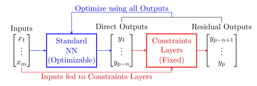
This NN, referred to as ACnet, calculates direct outputs using a standard NN while the remaining outputs are calculated as residuals from the fixed constraints layers, upstream of the optimizer. We summarize the $\mathrm{MSE\ }$and $\mathrm{Penalty}\$of UCnet, ACnet, and $\mathrm{LCnet}_{\alpha}\$of various weights $\alpha$ in Figure 2.

Fig. 2: Mean-squared error $\mathrm{MSE}$ (black) and squared-residual $\mathrm{Penalty}$ (blue) from conservation laws for UCnet, ACnet and $\mathrm{LCnet}_{\alpha}\$for $\alpha\in\left\{0,0.01,0.25,0.5,0.75,0.99,1\right\}$. Note that $\mathrm{LCnet}_{\alpha=0}=\mathrm{UCnet}$.

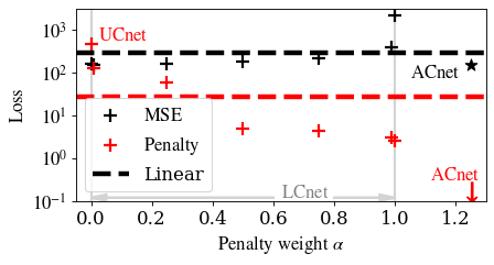
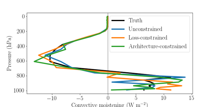
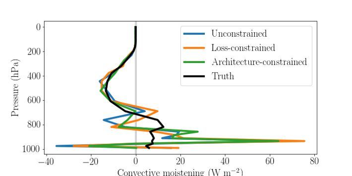
In this weak constraint perspective, we note a clear trade-off between performance (measured by $\mathrm{MSE}$) and physical constraints (measured by the $\mathrm{Penalty}$) as the weight $\alpha\$given to conservation laws increases from 0 to 1. An intermediate value is desirable (e.g., $\alpha=0.01\$or $\alpha=0.25$) as UCnet ($\mathrm{LCnet}_{\alpha=0}$) violates conservation laws more than the multiple-linear regression baseline (horizontal blue line) and $\mathrm{LCnet}_{\alpha=1}$ performs worse than the multiple-linear regression baseline (horizontal black line). In contrast, ACnet eliminates the need to compromise between performance and physical constraints by enforcing conservation laws to within machine precision, which is required in climate models, while achieving skill that is competitive with UCnet. Having solved the conservation issue, in the next section we turn to a deeper problem with NNs that, despite being physically-constrained, ACnets and LCnets both fail to generalize to unseen climates (Figure 3).

Fig. 3: Daily-averaged prediction from UCnet, $\mathrm{LCnet_{\alpha=0.01}}$, and ACnet in the Tropics for the reference climate (top) and the (+4K) experiment (bottom)

3 Improving Generalization to Unseen Climates

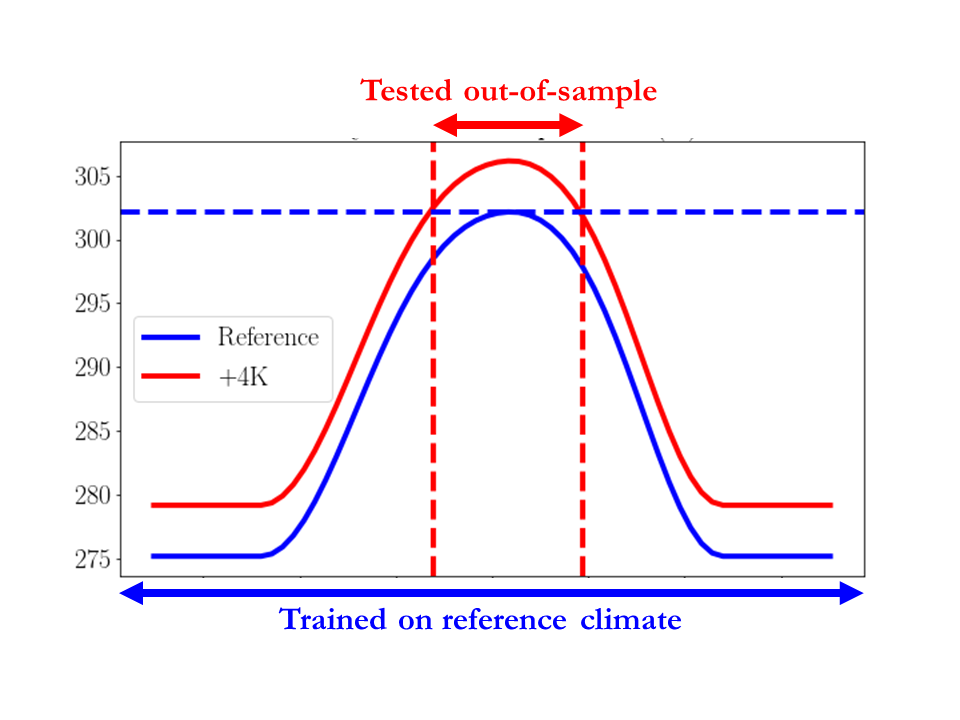
Testing generalization ability requires a generalization test. For that purpose, we run another SPCAM simulation after applying a uniform 4K warming to the surface temperature, which we will refer to as the (+4K) experiment. We then test the NNs trained on the reference climate in out-of-sample conditions, i.e. the deep Tropics of (+4K) as illustrated in SI Figure 5. As can be seen in Figure 3, NNs make extremely large errors when evaluated outside of their training set, such as overestimating convective moistening by a factor of 5.

Motivated by the success of non-dimensionalization to improve the generalizability of models in fluid mechanics, we seek to rephrase the boxed part of our convective parametrization ($\boxed{\boldsymbol{x}}\mapsto\boxed{\boldsymbol{y}}$) to improve its generalizability by using variables that have similar distributions in both climates. Unlike idealized problems in fluid mechanics, moist thermodynamics involve multiple non-linear processes, including phase changes and non-local interactions, which prevent reducing our mapping to a few dimensionless numbers. Instead, we develop a three-step method that consists of (1) non-dimensionalizing the input and output training datasets to then (2) train NNs on these new datasets to finally (3) compare their generalization abilities to our baseline UCnet. We use a different architecture of 7 layers with 128 neurons each for that lower-dimensional mapping, again informed by formal hyperparameter tuning, and train the NNs for 15 epochs using the Adam optimizer [17] while saving the state of best validation loss to avoid over-fitting.

Fig. 4: Daily-averaged predicted convective moistening (left) and heating (right) from UCnet (blue), a NN with scaled inputs (orange line) and a NN with scaled inputs and outputs (green) in the Tropics for the (+4K) experiment

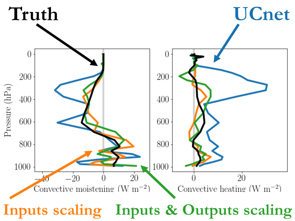
We make progress via trial-and-error of multiple NNs and present two successful rescalings below and in Figure 4: one for the inputs and one for the outputs.

Both successful rescalings leverage the Clausius-Clapeyron equation, which implies that the saturation specific humidity $q_{v}^{*}\$scales exponentially with absolute temperature $T$, making the extrapolation problem across climates especially challenging. The first rescaling (inputs) is to use relative humidity instead of specific humidity (orange vertical lines): $\boldsymbol{q_{v}}\mapsto\boldsymbol{RH}\approx\boldsymbol{q_{v}}/\boldsymbol{q_{v}^{*}}\left(T\right)$. This exploits the fact that unlike specific humidity, relative humidity is expected to change relatively little as the climate warms [18]. The second rescaling (outputs) is to normalize the vertical redistribution of energy by convection (in $\mathrm{W\ m^{-2}}$) using surface enthalpy fluxes conditionally averaged on temperature (green line, see SI Equations 7 and 8). Although both physically-motivated rescalings significantly improve the ability of the NN to generalize to unseen conditions, errors linked to the upwards shift of convection with warming are still visible in Figure 4. This motivates physically-rescaling the vertical coordinate, which we leave for future work.

Note that training a NN on both the reference climate and the (+4K) experiment would be the simplest way of achieving generalizability. However, the exercise of physically-rescaling the data to make our NN generalize to unseen climates (1) mimicks the present-day challenge of predicting the future climate based on observed statistics of the current climate, and (2) identifies the relevant physical rescalings to work towards a climate-invariant mapping from the local climate to convective tendencies.

4 Conclusion

We made progress towards physically-consistent neural-network parametrizations of convection in two ways. In Section 2, we enforced physical constraints in NNs (1) approximately by using the loss function and (2) to within machine precision by modifying the network’s architecture. In Section 3, we helped neural-networks generalize to unseen conditions by leveraging the Clausius-Clapeyron equation to physically rescale both inputs and outputs of the parametrization. While our work initially stemmed from operational requirements to improve convective processes in climate models, the generalization exercise of Section 3 also offers a pathway towards data-driven scientific discovery of the interaction between convection and the large-scale climate, e.g. to better adapt the entrainment-detrainment paradigm to diverse convective regimes or discover new equations to parameterize convection.

Supplemental Information

Variable	Name
$\mathrm{LHF}$	Latent heat flux
$\mathrm{\boldsymbol{LS}}$	Large-scale forcings in
	water, temperature, velocity
$\boldsymbol{\mathrm{lw}}$	Longwave heating rate profile
$\mathrm{LW_{s}}$	Net surface longwave flux
$\mathrm{LW_{t}}$	Net top-of-atmosphere longwave flux
$P$	Total precipitation rate
$P_{i}$	Solid precipitation rate
$p_{s}$	Surface pressure
$S_{0}$	Solar insolation
$\mathrm{SHF}$	Sensible heat flux
$\boldsymbol{\mathrm{sw}}$	Shortwave heating rate profile
$\mathrm{SW_{s}}$	Net surface shortwave flux
$\mathrm{SW_{t}}$	Net top-of-atmosphere shortwave flux
$\boldsymbol{T}$	Absolute temperature profile
$\boldsymbol{\dot{T}}$	Convective heating profile
$\boldsymbol{\dot{T}_{\mathrm{KE}}}$	Heating from turbulent
	kinetic energy dissipation
$\boldsymbol{q_{i}}$	Ice concentration profile
$\boldsymbol{\dot{q_{i}}}$	Convective ice tendency profile
$\boldsymbol{q_{l}}$	Liquid water concentration profile
$\boldsymbol{\dot{q_{l}}}$	Convective liquid water tendency profile
$\boldsymbol{q_{v}}$	Specific humidity profile
$\boldsymbol{\dot{q_{v}}}$	Convective water vapor tendency profile
$\boldsymbol{v}$	North-South velocity profile

Table 1: Definition of Variables: Variables that depend on height are (boldfaced) vectors, referred to as “profiles”.

Fig. 5: Surface temperature versus latitude for the reference and (+4K) experiments

Physically-rescaling the NN outputs

Motivated by the success of rescaling input data to take into account the sharp increase of atmospheric water vapor concentration with temperature, we develop an analogous normalization for the output data. As convection typically redistributes energy from the bottom to the top of the atmosphere, we can interpret convective heating and moistening profiles as processes partitioning surface enthalpy fluxes (in $\mathrm{W\ m^{-2}}$) between different layers of the atmosphere. As such, we mass-weight both profiles before rescaling them using surface enthalpy fluxes conditionally-averaged on near-surface temperature (referred to as $\mathrm{SEF\left(T_{NS}\right)}$). Mathematically, this physical rescaling can be written as:

$$\boldsymbol{\dot{q}_{v}}\left[\mathrm{kg/kg}/s\right]\mapsto\frac{L_{v}\boldsymbol{\Delta p}}{g\times\mathrm{SEF}\left(T_{\mathrm{NS}}\right)}\boldsymbol{\dot{q}_{v}}\ \left[1\right],$$ (7)

$$\boldsymbol{\dot{T}}\left[K/s\right]\mapsto\frac{c_{p}\boldsymbol{\Delta p}}{g\times\mathrm{SEF}\left(T_{\mathrm{NS}}\right)}\boldsymbol{\dot{T}}\ \left[1\right],$$ (8)

where $\boldsymbol{\Delta p}\$are the layers’ pressure thicknesses, $g\$is the gravity constant, $c_{p}\$is the specific heat capacity of dry air at constant pressure, and $L_{v}\$is the latent heat of vaporization of water in standard atmospheric conditions.

References

- [1] Tapio Schneider, João Teixeira, Christopher S. Bretherton, Florent Brient, Kyle G. Pressel, Christoph Schär, and A. Pier Siebesma, “Climate goals and computing the future of clouds,” Nature Climate Change, vol. 7, no. 1, pp. 3–5, 2017.
- [2] C L Daleu, R S Plant, S J Woolnough, S Sessions, M J Herman, A Sobel, S Wang, D Kim, A Cheng, G Bellon, P Peyrille, F Ferry, P Siebesma, and L. Van Ulft, “Intercomparison of methods of coupling between convection and large-scale circulation: 2. Comparison over nonuniform surface conditions,” Journal of Advances in Modeling Earth Systems, vol. 8, no. 1, pp. 387–405, mar 2016.
- [3] IPCC, Climate Change 2013 - The Physical Science Basis, Cambridge, United KingdomNew York, NY, USA, cambridge edition, 2014.
- [4] P. Gentine, M. Pritchard, S. Rasp, G. Reinaudi, and G. Yacalis, “Could Machine Learning Break the Convection Parameterization Deadlock?,” Geophysical Research Letters, vol. 45, no. 11, pp. 5742–5751, jun 2018.
- [5] Paul A. O’Gorman and John G. Dwyer, “Using Machine Learning to Parameterize Moist Convection: Potential for Modeling of Climate, Climate Change, and Extreme Events,” 2018.
- [6] Noah D Brenowitz and Christopher S Bretherton, “Spatially Extended Tests of a Neural Network Parametrization Trained by Coarse-Graining,” Journal of Advances in Modeling Earth Systems, vol. 11, no. 8, pp. 2728–2744, apr 2019.
- [7] Noah Domino Brenowitz and Christopher Stephen Bretherton, “Prognostic Validation of a Neural Network Unified Physics Parameterization,” Geophysical Research Letters, vol. 45, no. 12, pp. 6289–6298, 2018.
- [8] Stephan Rasp, Michael S Pritchard, and Pierre Gentine, “Deep learning to represent sub-grid processes in climate models,” Proceedings of the National Academy of Sciences of the United States of America, vol. 115, no. 39, pp. 9684–9689, sep 2018.
- [9] Tom Beucler, Stephan Rasp, Michael Pritchard, and Pierre Gentine, “Achieving Conservation of Energy in Neural Network Emulators for Climate Modeling,” 2019.
- [10] Tom Beucler, Michael Pritchard, Stephan Rasp, Pierre Gentine, Jordan Ott, and Pierre Baldi, “Enforcing Analytic Constraints in Neural-Networks Emulating Physical Systems,” sep 2019.
- [11] Marat Khairoutdinov, David Randall, and Charlotte DeMott, “Simulations of the Atmospheric General Circulation Using a Cloud-Resolving Model as a Superparameterization of Physical Processes,” Journal of the Atmospheric Sciences, vol. 62, no. 7, pp. 2136–2154, jul 2005.
- [12] Michael S. Pritchard, Christopher S. Bretherton, and Charlotte A. Demott, “Restricting 32-128 km horizontal scales hardly affects the MJO in the Superparameterized Community Atmosphere Model v.3.0 but the number of cloud-resolving grid columns constrains vertical mixing,” Journal of Advances in Modeling Earth Systems, vol. 6, no. 3, pp. 723–739, sep 2014.
- [13] Lars Hertel, Peter Sadowski, Julian Collado, and Pierre Baldi, “Sherpa : Hyperparameter Optimization for Machine Learning Models,” Conference on Neural Information Processing Systems (NIPS), , no. Nips, oct 2018.
- [14] Tijmen Tieleman, Geoffrey E. Hinton, Nitish Srivastava, and Kevin Swersky, “Lecture 6.5-rmsprop: Divide the gradient by a running average of its recent magnitude,” COURSERA: Neural Networks for Machine Learning, vol. 4, no. 2, pp. 26—-31, 2012.
- [15] Anuj Karpatne, William Watkins, Jordan Read, and Vipin Kumar, “Physics-guided Neural Networks (PGNN): An Application in Lake Temperature Modeling,” 2017.
- [16] Xiaowei Jia, Jared Willard, Anuj Karpatne, Jordan Read, Jacob Zwart, Michael Steinbach, and Vipin Kumar, “Physics guided RNNs for modeling dynamical systems: A case study in simulating lake temperature profiles,” in SIAM International Conference on Data Mining, SDM 2019, 2019, pp. 558–566.
- [17] Diederik P. Kingma and Jimmy Ba, “Adam: A Method for Stochastic Optimization,” dec 2014.
- [18] David M. Romps, “An analytical model for tropical relative humidity,” Journal of Climate, vol. 27, no. 19, pp. 7432–7449, 2014.