Abstract

In this work, we study the event occurrences of individuals interacting in a network. To characterize the dynamic interactions among the individuals, we propose a group network Hawkes process (GNHP) model whose network structure is observed and fixed. In particular, we introduce a latent group structure among individuals to account for the heterogeneous user-specific characteristics. A maximum likelihood approach is proposed to simultaneously cluster individuals in the network and estimate model parameters. A fast EM algorithm is subsequently developed by utilizing the branching representation of the proposed GNHP model. Theoretical properties of the resulting estimators of group memberships and model parameters are investigated under both settings when the number of latent groups $G$ is over-specified or correctly specified. A data-driven criterion that can consistently identify the true $G$ under mild conditions is derived. Extensive simulation studies and an application to a data set collected from Sina Weibo are used to illustrate the effectiveness of the proposed methodology.

KEY WORDS: EM algorithm; Latent group structure; Multivariate Hawkes process; Network data analysis.

1 INTRODUCTION

Point process models have gained increasing popularity for modeling activities observed on various networks, examples include posting activities in online social networks, corporation transactions in a financial network, and neuron spikes in a brain network. The main goal of this work is to develop a new modeling framework for random event times observed on a network consisting of heterogeneous nodes. While the proposed framework is applicable for the analysis of general event time data, we describe our model in the context of a motivating dataset collected from Sina Weibo (the largest Twitter type social media platform in mainland China).

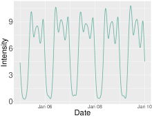
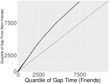
The dataset contains posting times of 2,038 Sina Weibo users from January 1st to January 15th, 2014. Figure 1 shows that user posting patterns be highly heterogeneous and complex. Firstly, the distribution of user post counts reveals great variability in users’ activities levels: while most users had less than 200 posts during the study period, a small portion of users were much more active. Secondly, the averaged overall intensity of posting times aggregated over all users demonstrates the existence of apparent daily periodic patterns. Lastly, quantiles of gap times between a user’s posting time and the closest posting time from his/her connected friends and randomly picked non-friends are drastically different. In particular, the quantiles of gap times among friends are consistently smaller than those among the non-friends, suggesting that a user’s activities were heavily influenced by his/her friends.

Figure 1: Left: histogram of users’ post counts. Middle: estimated overall intensity function of all users’ posting times. Right: QQ-plot of gap times among friends and among random picked non-friends.

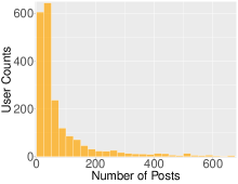
A popular model for event time data such as our motivating example is the multivariate Hawkes process (Hawkes, 1971), which has been widely used to model event times of multiple types in a variety of fields, such as criminology (Linderman and Adams, 2014), finance (Bacry et al., 2013), information diffusion (Farajtabar et al., 2017), and social studies (Zhou et al., 2013; Fox et al., 2016). In the network setting, the first line of existing research aims at recovering the unknown network structure using the observed event time data, see, e.g., Zhou et al. (2013); Xu et al. (2016); Achab et al. (2018); Bacry et al. (2020). In contrast, another line of research takes the network structure as given knowledge and incorporates it into the modeling of the event time data, examples include Fox et al. (2016); Farajtabar et al. (2017) and Zarezade et al. (2018). In the second framework, model parameters were assumed to be node-specific, and therefore the number of parameters grows at least linearly with the number of nodes. This may be problematic if many nodes in the network produce only scarce event times, which was observed in Figure 1. Section 2.4 gives a more detailed comparison between the proposed model and existing works.

In this work, we propose a group network Hawkes process (GNHP) to model the network heterogeneity by introducing a latent group structure among the network nodes. We assume that nodes in the same group share similar node-wise characteristics and that interaction patterns between any two connected nodes are determined by their group memberships. For each latent group, the background intensity varies over time and is nonparametrically approximated by spline basis functions. The proposed model is more parsimonious than existing models where all network nodes are considered as different (e.g., Fox et al., 2016; Farajtabar et al., 2017; Zarezade et al., 2018), but the latent group structure coupled with the observed network structure still allows us to build sufficiently flexible multivariate Hawkes process network models. Furthermore, the proposed GNHP model admits an equivalent branching process structure that enables us to develop easily interpretable numerical measures to quantify interactions within the network, see Section 2.3 for more details. The branching structure also allows us to develop a computationally efficient EM algorithm for model estimation, see Section 3.3. Lastly, the estimated group memberships cluster network nodes into several subgroups in a data-driven manner, offering further insights into the network activity dynamics. Therefore, the proposed GNHP model is an important addition to the existing toolbox for analyzing event time data observed on a network.

Our work also makes important theoretical contributions to the literature. The estimation of the (multivariate) Hawkes process is most commonly conducted through the maximum likelihood estimation (Ogata, 1988; Mohler et al., 2011; Chen and Hall, 2013; Zhou et al., 2013). While Ogata (1978) and Chen and Hall (2013) studied the asymptotic property of the maximum likelihood estimator (MLE) for a univariate Hawkes process, to the best of our knowledge, however, little is known about the limiting behaviors of the MLE for a high-dimensional multivariate Hawkes process such as the proposed GNHP. In this work, we establish the consistency results for the MLE of the model parameters and the latent group memberships for the GNHP, with the number of groups being possibly over-specified. When the number of groups is correctly specified, we establish the asymptotic normality of the MLE. Finally, we show that a likelihood-based information criterion (LIC) can consistently select the number of groups. A similar theoretical framework has been considered in the panel data literature (Su et al., 2016; Liu et al., 2020; Zhu et al., 2022), although the treatments of point process data and panel data are very different. In this sense, our work also bridges a gap between the point process and the panel data literature.

The rest of the article is organized as follows. In Section 2, we introduce the GNHP model together with its branching structure representation and compare the proposed model to existing works. In Section 3, we detail our estimation procedure, including the computationally efficient EM algorithm. Theoretical properties of resulting estimators are investigated in Section 4. Simulation results under different network settings are presented in Section 5. In Section 6, we apply the proposed model to the Sina Weibo dataset. The article is concluded with a brief discussion in Section 7. Additional simulation resulats and all technical details are left to online supplementary material.

2 GROUP NETWORK HAWKES PROCESS

2.1 Background on Hawkes Process

Denote by $0\leq t_{1}\leq t_{2}\leq\ldots\leq t_{n}\leq T$ a realization of a temporal point process in $[0,T]$ and let $N(t)=\sum_{k=1}^{n}{I}(t_{k}<t)$ be the associated counting process, where ${I}(\cdot)$ is an indicator function. Let $\mathcal{H}_{t}=\{t_{k}:t_{k}<t\}$ be the process history up to time $t$, and the conditional intensity function of a point process is defined as $\lambda(t|\mathcal{H}_{t})=\underset{\Delta\rightarrow 0}{\mathrm{lim}}\Delta^{-1}{\mbox{$\mathbb{E}$}\left[N(t+\Delta)-N(t)|\mathcal{H}_{t}\right]}.$ The classical Hawkes process model (Hawkes, 1971) assumes that $\lambda(t|\mathcal{H}_{t})$ takes the form

$$\lambda(t|\mathcal{H}_{t})=\mu+\sum_{t_{k}\in\mathcal{H}_{t}}f(t-t_{k}),$$ (1)

where $\mu>0$ is a background rate of events and $f(\cdot)$ is a non-negative triggering function. The Hawkes process is considered as “self-exciting” since the past events in $\mathcal{H}_{t}$ contribute to the instantaneous intensity $\lambda(t|\mathcal{H}_{t})$ at time $t$ through $f(\cdot)$. The triggering function controls the dependence range and strength between the intensity at time $t$ and the past events, and popular choices include the exponential kernel (Hawkes, 1971) and the power-law kernel (Ogata, 1988).

Notations. For a vector $\mathbf{v}=(v_{1},\cdots,v_{p})^{\top}\in\mathbb{R}^{p}$, let $\|\mathbf{v}\|_{2}=(\sum_{i=1}^{p}v_{i}^{2})^{1/2}$ and $\|\mathbf{v}\|_{\infty}=\max_{j}|v_{j}|$ denote the $L_{2}$-norm and the infinity norm of $\mathbf{v}$, respectively. For a function $h(t)\in\mathbb{R}^{1}$ with $t\in[0,T]$, define $\|h(\cdot)\|_{T}=\{T^{-1}\int_{0}^{T}h(t)^{2}dt\}^{1/2}$ and $\|h(\cdot)\|_{\infty}=\sup_{t\in[0,T]}|h(t)|$. For a matrix ${\bf H}=(h_{ij})\in\mathbb{R}^{m\times n}$, define the row norm $\|{\bf H}\|_{\infty}=\max_{i}(\sum_{j}|h_{ij}|)$ and $L_{1}$ norm $\|{\bf H}\|_{1}=\sum_{i}(\sum_{j}|h_{ij}|)$. For any set $\mathcal{S}$, define $\mathcal{S}^{n}=\{\mathbf{v}=(v_{1},\cdots,v_{n})^{\top}:v_{i}\in\mathcal{S}\}$ as collection of vectors of length $n$, whose elements are in $\mathcal{S}$. Finally, we denote $[G]=\{1,\cdots,G\}$ and ${\bf 1}=(1,\cdots,1)^{\top}$.

2.2 Network Hawkes Process with Latent Group Structures

In this section, we extend the classical Hawkes process to the network setting with a latent group structure. Consider a network with $m$ nodes, where the relationships among the nodes are represented by an adjacency matrix $A=(a_{ij})\in\mathbb{R}^{m\times m}$, with $a_{ij}=1$ if the $i$th node follows the $j$th node and $a_{ij}=0$ if otherwise. By convention, we do not allow self-connected nodes, i.e., $a_{ii}=0$. To account for potential heterogeneity of network nodes, we assume that the nodes in the network belong to $G$ latent groups where nodes within the same group share the same node-specific characteristics and interactions with nodes from other groups.

Denote $\mathscr{G}=(g_{1},\cdots,g_{m})^{\top}\in\mathbb{R}^{m}$ as the latent group membership vector of all nodes, where $g_{i}\in[G]$ for $i=1,\cdots,m$. For node $i$, let $0\leq t_{i1}\leq t_{i2}\leq\cdots\leq t_{in_{i}}\leq T$ be the observed $n_{i}$ event times and $N_{i}(t)=\sum_{k=1}^{n_{i}}I(t_{ik}\leq t)$ be the associated counting process. Given the group membership vector $\mathscr{G}$ and event history $\mathcal{H}_{t}=\cup_{i=1}^{m}\mathcal{H}_{i,t}$ with $\mathcal{H}_{i,t}=\{t_{ik}:t_{ik}<t;1\leq k\leq n_{i}\}$, the proposed GNHP model assumes that the conditional intensity for the $i$th node is of the form

$$\lambda_{i}(t|\mathscr{G},\mathcal{H}_{t})=\mu_{g_{i}}(t)+\beta_{g_{i}}\sum_{t_{ik}\in\mathcal{H}_{i,t}}f_{b}(t-t_{ik};\eta_{g_{i}})+\sum_{j=1}^{m}\phi_{g_{i}g_{j}}\frac{a_{ij}}{d_{i}}\sum_{t_{jl}\in\mathcal{H}_{j,t}}f_{b}(t-t_{jl};\gamma_{g_{i}}),$$ (2)

for $1\leq i\leq m$, where $\mu_{g}(\cdot)$ is the background intensity, $f_{b}(\cdot;\eta)$ is a triggering function governed by parameter $\eta$, $d_{i}=\sum_{j=1}^{m}a_{ij}$ is the out-degree of node $i$ (Zhu et al., 2017), and $\{\beta_{g},\gamma_{g},\eta_{g},\phi_{gg^{\prime}}\}$ are unknown group-level parameters for $g,g^{\prime}\in[G]$. Following Chen et al. (2017), we assume the support of $f_{b}(t;\gamma)$ is $[0,b]$. For example, $f_{b}(\cdot;\gamma)$ can be the truncated exponential kernel

$$f_{b}(t;\gamma)=\gamma\left[1-\exp(-b\gamma)\right]^{-1}\exp(-\gamma t)I(t\leq b),\quad\text{ for any }t\geq 0.$$ (3)

Our theoretical investigation allows the truncation range $b\to\infty$ as $m,T\to\infty$. For identifiability of parameters $\beta_{g}$’s and $\phi_{gg^{\prime}}$’s, we assume that $\int_{0}^{\infty}f_{b}(t;\gamma)dt=1$ for any given $\gamma$. In addition, we assume that $\|\partial^{k}f_{b}(\cdot;\gamma)/\partial\gamma^{k}\|_{\infty}<\infty$ for $1\leq k\leq 3$.

The proposed conditional intensity in (2) can be decomposed into the following three parts.

• Background intensity $\mu_{g_{i}}(t)$. This describes the overall activity pattern of the node $i$.

• Momentum intensity $\beta_{g_{i}}\sum_{t_{ik}\in\mathcal{H}_{i,t}}f_{b}(t-t_{ik};\eta_{g_{i}})$. It models “self-exciting” influence of its own past events on the occurrence of a new event at $t$ at the node $i$.

• Network intensity $d_{i}^{-1}\sum_{j=1}^{m}\phi_{g_{i}g_{j}}a_{ij}\sum_{t_{jl}\in\mathcal{H}_{j,t}}f_{b}(t-t_{jl};\gamma_{g_{i}})$. This models influences from past events of other nodes on the occurrence of a new event at $t$ at node $i$.

The out-degree $d_{i}$ is used to prevent the inflation of the Network Intensity when $d_{i}\to\infty$, which is commonly done in literature (Zhu et al., 2017, 2019). The $\phi_{g_{i}g_{j}}$’s in the Network Intensity represent the average network influences from the connected nodes on the $i$th node. Finally, we remark that the triggering functions in the Momentum Intensity and the Network Intensity do not necessarily share the same form.

The network dependence of the proposed GNHP can be characterized by the transition matrix ${\bf B}=(b_{ij})\in\mathbb{R}^{m\times m}$, where $b_{ij}=\phi_{g_{i}g_{j}}d_{i}^{-1}a_{ij}+\beta_{g_{i}}I(i=j)$, for $i,j=1,\cdots,m.$ Detailed properties of ${\bf B}$ will be further explored in the next subsection based on the following assumption.

Assumption 1.

Assume $\|\mathbf{B}\|_{\infty}\leq c_{B}<1$, where $c_{B}$ is a positive constant.

Assumption 1 is a sufficient condition for stability of a multivariate Hawkes process and has been widely used in the literature, see, e.g., Hansen et al. (2015); Chen et al. (2017). In the next subsection, we show that for the GNHP model, it is a sufficient condition to ensure that the expected number of offspring events triggered by a parent event at any network node is finite.

2.3 Branching Structure of the GNHP Model

Hawkes and Oakes (1974) provides an equivalent branching structure representation for the classical Hawkes process (1), which classifies the observed events into two disjoint processes: a parent Poisson process with a rate $\mu$, and offspring processes triggered by past events. The branching structure of the classical Hawkes process is illustrated in the left panel of Figure 2.

Figure 2: Branching structures of the classical Hawkes process (left) and the GNHP (right). Left: parent events (blue circle) and two generations of offspring events; Right: a two-node network where Node 1 follows Node 2. Parent events from both nodes (blue circles), event times triggered by their own past events (purple circles), event times in Node 1 triggered by past events from Node 2 (green circles).

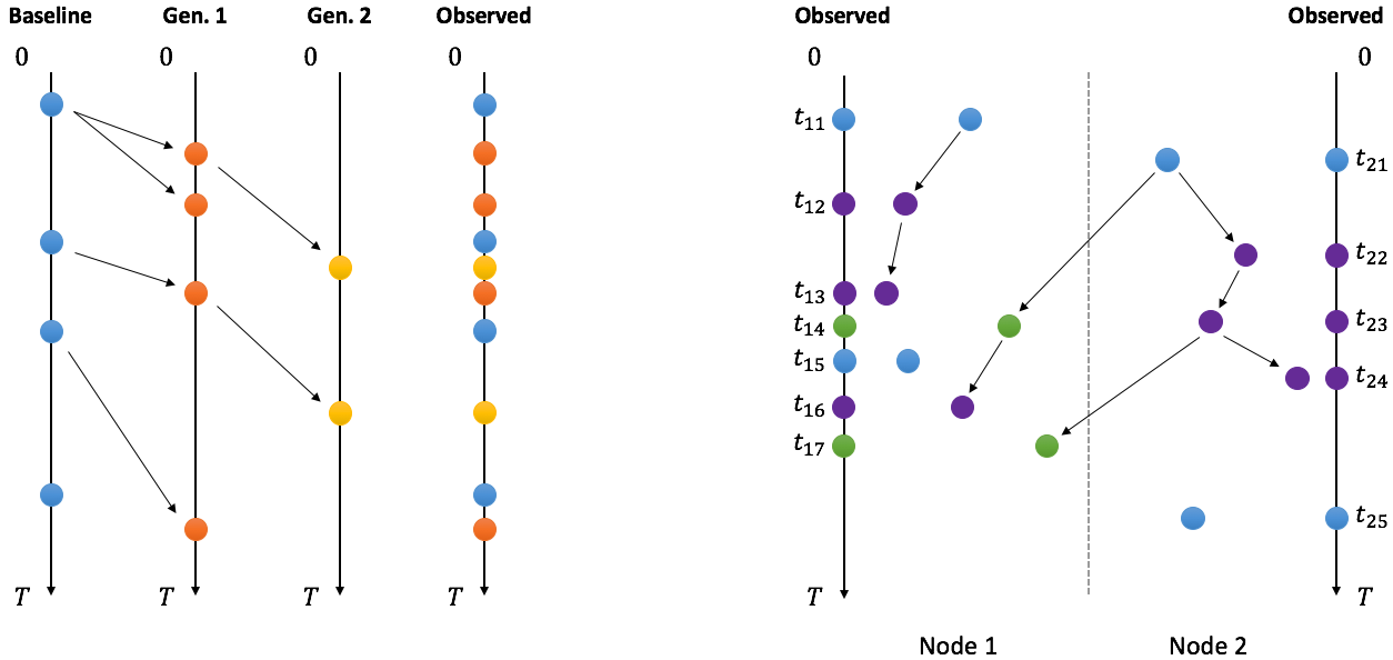
Following Rasmussen (2013) and Halpin et al. (2013), a branching structure representation can be derived for the GNHP by treating the aggregated point process from all nodes, denoted by $N^{\rm pool}$, as a marked point process on $[0,T]$, with the mark for any $t\in N^{\rm pool}$ being the node index where the event occurs. Specifically, event times in $N^{\rm pool}$ can be categorized into two types: the parent and offspring events. Let $\mathcal{M}_{i}^{parent}$ be the set of parent events from node $i$ and $\mathcal{M}_{ik}^{fam}=\mathcal{M}_{ik}^{off}\cup\{t_{ik}\}$, where $\mathcal{M}_{ik}^{off}$ is the set of offspring events generated from a parent event $t_{ik}\in\mathcal{M}_{i}^{parent}$. Note that $\mathcal{M}_{ik}^{fam}$ may contain event times from other nodes due to the network interactions. The branching structure is defined as follows and illustrated in Figure 2.

1. For any $1\leq i\leq m,$ the parent events $\mathcal{M}_{i}^{parent}$ follows a Poisson process with an intensity $\mu_{g_{i}}(t)$, and all Poisson processes are independent.

2. Each parent event $t_{ik}\in\mathcal{M}_{i}^{parent}$ generates a set of offspring events $\mathcal{M}_{ik}^{off}$, and all resulting $\mathcal{M}_{ik}^{fam}$’s are independent. Event times in each $\mathcal{M}_{ik}^{fam}$ are generated recursively as follows.

   1. Generation $0$, denoted as $\mathcal{M}_{ik}^{gen_{0}}$, consists of only $t_{ik}$, i.e., $\mathcal{M}_{ik}^{gen_{0}}=\{t_{ik}\}$.

   2. Having generated offspring event times up to $n$ generations, $\mathcal{M}_{ik}^{gen_{0}},\cdots,\mathcal{M}_{ik}^{gen_{n}}$, each event time in $\mathcal{M}_{ik}^{gen_{n}}$ generates a series of event times of the $n+1$ generation. Specifically, suppose $t_{jl}\in\mathcal{M}_{ik}^{gen_{n}}$ is an event time located in the $j$th node, then on the time interval $[t_{jl},T]$, it generates (i) a Poisson process with intensity $\beta_{g_{j}}f_{b}(t-t_{jl};\eta_{g_{j}})$ on the node $j$; and (ii) a Poisson process with intensity $\phi_{g_{i^{\prime}}g_{j}}d_{i^{\prime}}^{-1}f_{b}(t-t_{jl};\gamma_{g_{i^{\prime}}})$ on the node $i^{\prime}$ for any $i^{\prime}\neq j$ where $a_{i^{\prime}j}=1$. All Poisson processes are independent.

   3. Obtain $\mathcal{M}_{ik}^{fam}=\cup_{n=0}^{\infty}\mathcal{M}_{ik}^{gen_{n}}$.

Theorem 1.

Denote by $\#_{i}(\mathcal{S})$ the total number of events occurring at a subset of network nodes $\mathcal{S}\subset\{1,\cdots,m\}$ that are offspring events of a parent event originated from the $i$th node on $[0,\infty)$. Then under Assumption 1, one has that

$$E\left[\#_{i}(\mathcal{S})\right]={\bf e}_{\mathcal{S}}^{\top}({\bf I}-{\bf B})^{-1}{\bf e}_{i},\text{ for any }1\leq i\leq m,$$ (4)

where ${\bf e}_{\mathcal{S}}$ is a vector with $1$ for entries whose indexes are in $\mathcal{S}$ and $0$ elsewhere, and ${\bf e}_{i}={\bf e}_{\{i\}}$.

The proof is given in the online supplement. Theorem 1 provides a useful tool to quantify the network interactions. Examples include

• Node-to-node influence: the $(j,i)$th entry of $({\bf I}-{\bf B})^{-1}$ gives the average number of events at node $j$ that are triggered by a parent event at the $i$th node (set $\mathcal{S}=\{j\}$).

• Node-to-network influence: by setting $\mathcal{S}=\{1,\cdots,m\}$, we obtain the sum of the $i$th column of $({\bf I}-{\bf B})^{-1}$ as the average number of events in the entire network that are directly/indirectly triggered by a parent event at the $i$th node, i.e., $E\{\#_{i}(\mathcal{S})\}=E\{|\mathcal{M}_{ik}^{fam}|\}$.

• Dynamic Group-to-Group influence: Let $\mathcal{S}_{g}$ be the collection of node indexes in group $g$. Denote $\#(\mathcal{S}_{g},\mathcal{S}_{g^{\prime}},[t_{1},t_{2}])$ as the total number of events from group $g^{\prime}$ triggered by parent events from group $g$ occurring within $[t_{1},t_{2}]$, which reflects the influential power of group $g$ on group $g^{\prime}$. Based on Theorem 1, it can be verified that $E\Big{\{}\#(\mathcal{S}_{g},\mathcal{S}_{g^{\prime}},[t_{1},t_{2}])\Big{\}}={\bf e}_{\mathcal{S}_{g^{\prime}}}^{\top}({\bf I}-{\bf B})^{-1}{\bf e}_{\mathcal{S}_{g}}\int_{t_{1}}^{t_{2}}\mu_{g}(t)dt$. We can subsequently define the limiting case as follows

  $${\rm GIF}_{gg^{\prime}}(t)=\lim_{\Delta\to 0}{\Delta^{-1}}E\Big{\{}\#(\mathcal{S}_{g},\mathcal{S}_{g^{\prime}},[t,t+\Delta])\Big{\}}={\bf e}_{\mathcal{S}_{g^{\prime}}}^{\top}({\bf I}-{\bf B})^{-1}{\bf e}_{\mathcal{S}_{g}}\mu_{g}(t),\quad t\in[0,T],$$ (5)

  which is more convenient for graphical illustrations.

2.4 Comparisons with Existing Literature

There has been much work on multivariate Hawkes process (e.g., Zhou et al., 2013; Bacry et al., 2013; Chen et al., 2017), and models for the conditional intensity can be generally expressed as

$$\lambda_{i}(t|\mathscr{G},\mathcal{H}_{t})=\mu_{i}+\sum_{j=1}^{m}\sum_{t_{jl}\in\mathcal{H}_{j,t}}\zeta_{ij}(t-t_{jl}),\quad i=1,\cdots,m,$$ (6)

where $\mu_{i}$ is the background rate at node $i$ and $\zeta_{ij}(\cdot)$ is some transfer function between node $j$ and node $i$. Key differences among existing multivariate Hawkes process models center around constructions of $\zeta_{ij}(\cdot)$’s. A popular modeling strategy is to assume that $\zeta_{ij}(\cdot)=\theta_{ij}f(\cdot;\gamma)$, $i,j=1,\cdots,m$, with some parametric $f(\cdot;\gamma)$. Such a model involves a total of $O(m^{2})$ parameters, limiting its suitability to applications with a relatively small $m$ (e.g., Bacry et al., 2013). When modeling a large network, one needs to impose some sparse structure on $\theta_{ij}$’s, in which case a nonzero $\theta_{ij}$ implies that node $i$ is directly influenced by node $j$, and estimated $\theta_{ij}$’s may help recover the latent network structure (e.g., Xu et al., 2016; Bacry et al., 2020). While most work in this line lack rigorous theory, there has been some recent theoretical studies of such models when $m$ is diverging, see, e.g., Hansen et al. (2015), Chen et al. (2017) and Cai et al. (2020).

There is also a large body of literature on the identification of network node clusters (e.g., Zhao et al., 2012; Amini et al., 2013), which is commonly referred to as “community detection”. We remark that the concept of “community” in the community detection literature is fundamentally different from the “groups” in the proposed GNHP model. In community detection, the network adjacent matrix $A$ is assumed to be a random matrix consisting of Bernoulli random variables, and the identification of node communities $\mathbf{c}$ critically depends on the conditional probability $P(A|\mathbf{c})$. However, the adjacent matrix $A$ in the GNHP is considered deterministic and there is no probability associated with it. In contrast, the groups in the GNHP are formed by maximizing the likelihood of event times collected from all network nodes, and nodes in the same group are forced to share similar node-specific characteristics such as $\mu_{g_{i}}(\cdot)$’s and $\beta_{g_{i}}$’s. Although some recent works in community detection literature utilize nodal features to help identify communities (Yan and Sarkar, 2021; Zhang et al., 2021; Weng and Feng, 2022), the central piece of these models remains to be $P(A|\mathbf{c})$. The difference is most manifested in the extreme case when all nodes are isolated from each other (i.e., $A$ consists of all $0$’s), while the GNHP is still valid by manually setting $\phi_{g_{i}g_{j}}$’s as $0$, the community detection can no longer be performed since there is no network anymore. We note another recent work Matias et al. (2018) also considers latent group structures when extending the stochastic block model for recurrent interaction events in continuous time. The key difference between their work and ours lies in that they require that each observed event time is associated with a label indicating this event is an interaction between which two nodes. However, such information is not available in event times modeled by the GNHP, which instead focuses on modeling events that occur on individual nodes but may have some correlations. In fact, as suggested by the branching structure in Section 2.3, identifying the triggering source of an event in the GNHP is the most challenging task. Similarly, in the extreme case when there are only self-activities on each node but no interaction between any pair of nodes, Matias et al. (2018) is not applicable but the GNHP model remains valid with $\phi_{g_{i}g_{j}}$’s set to $0$.

The second line of research focuses on analyzing the network activities through parameterizations utilizing a known network structure, (e.g., Fox et al., 2016; Farajtabar et al., 2017; Zarezade et al., 2018). For instance, Fox et al. (2016) models email communications in a network by assuming $\zeta_{ij}(t)=\theta_{i}a_{ij}\gamma_{i}\exp(-\gamma_{i}t)$, where $\theta_{i}$’s and $\gamma_{i}$’s are unknown parameters. As a result, the total number of unknown parameters is reduced to $O(m)$. Similar but more complex models were studied in Farajtabar et al. (2017) and Zarezade et al. (2018).

Our proposed GNHP model falls into the second line of research with four distinct features: (a) the background intensities $\mu_{i}(\cdot)$’s are allowed to be time-varying and nonparametrically approximated using spline basis functions, which provides greater modeling flexibility. (b) the Momentum Intensity in model (2) has a clear interpretation given the network structure. (c) the latent group structure imposed on network nodes not only accounts for commonly observed network heterogeneity in a natural way but also effectively reduces the number of parameters. (d) the estimated group memberships for network nodes may provide further insights on the network activities using various influence measures discussed in Section 2.3.

3 MODEL ESTIMATION

3.1 Background Intensity Approximation

As illustrated in Figure 1, human activities such as social media posting often exhibit periodic patterns. We, therefore, assume that the background intensity of a given node takes a periodic form, for which there exists a finite $\omega>0$ such that $\mu_{g}(t)=\mu_{g}(t+l\omega)$, $t\in[0,T-l\omega]$, $l=0,1,2,\cdots,$ for any $g\in[G]$. For our motivating example, it is natural to choose $\omega=1$ day (or $24$ hours) to account for daily posting behaviors. Without assuming a restrictive parametric form for $\mu_{g}(\cdot)$’s, we approximate $\mu_{g}(\cdot)$ using periodic splines. Let ${\bf k}_{n_{\rm kt}}(\cdot)=(k_{1}(\cdot),\cdots,k_{n_{\rm kt}}(\cdot))^{\top}$ be a collection of basis functions defined on $[0,\omega]$ and ${\bf x}_{n_{\rm kt}}(t)=\sqrt{n_{\rm kt}}{\bf k}_{n_{\rm kt}}(t-\lfloor t/\omega\rfloor{\omega})$ for any $t\in[0,T]$, where $\lfloor a\rfloor$ is the largest integer less than or equal to $a$, then $\mu_{g}(\cdot)$ is approximated by

$$\mu_{g}(t)=\mathbf{w}_{g}^{\top}{\bf x}_{n_{\rm kt}}(t),\quad t\in[0,T],$$ (7)

where $\mathbf{w}_{g}$, $g\in[G]$, are the coefficient vectors that need to be estimated. For our theoretical investigation, we require the following assumption for the spline basis functions.

Assumption 2.

Assume that there exists a constant $R>0$ such that $k_{1}(\cdot),\cdots,k_{n_{\rm kt}}(\cdot)$ satisfy: (a) $\|k_{j}(\cdot)\|_{\infty}\leq R$ and $\int_{0}^{\omega}|k_{j}(t)|dt=O(n_{\rm kt}^{-1})$; (b) $\int_{0}^{\omega}|k_{j}(t)k_{j+l}(t)|dt=O(n_{\rm kt}^{-1})$, and $k_{j}(t)k_{j+l}(t)=0$ for $l>J$ and any $t\in[0,\omega]$, where $J\geq 0$ is a finite integer. Denote by $\mu^{0}_{g}(\cdot)$ the true background function of group $g$, and assume that for some constant $\nu>0$, it holds that

$$\max_{1\leq g\leq G}\inf_{\mathbf{w}_{g}\in\mathbb{R}^{n_{\rm kt}},\|\mathbf{w}_{g}\|_{\infty}\leq R/\sqrt{n_{\rm kt}}}\big{\|}\mu_{g}^{0}(\cdot)-\mathbf{w}_{g}^{\top}{\bf x}_{n_{\rm kt}}(\cdot)\big{\|}_{\infty}=O(n_{\rm kt}^{-\nu}).$$ (8)

Assumption 2 requires that the true background intensity functions can be approximated sufficiently well by a linear combination of spline basis functions, which is mild for many spline families. In our numerical examples, we choose $k_{1}(\cdot),\cdots,k_{n_{\rm kt}}(\cdot)$ as the $r$th-order B-spline basis functions with equally spaced knots on $[0,\omega]$, which meet Assumption 2 (Zhou et al., 1998).

3.2 Maximum Likelihood Estimation

For any $g\neq g^{\prime}$, denote $\mathbb{W}\subset\mathbb{R}^{n_{\rm kt}}$, $\boldsymbol{\Theta}\subset\mathbb{R}^{+3}$ and $\boldsymbol{\Phi}\subset\mathbb{R}^{+}$ as the parameter spaces for parameters in $\mathbf{w}_{g}$, $\boldsymbol{\theta}_{g}=(\beta_{g},\eta_{g},\gamma_{g})^{\top}$, and $\phi_{gg^{\prime}}$’s, respectively. Here $\mathbb{R}^{+}$ denotes $[0,\infty)$. Denote by $\mathbb{G}\equiv[G]^{m}$ as the parameter space for the membership vector $\mathscr{G}=(g_{1},\cdots,g_{m})^{\top}$. For our theoretical investigation, we impose the following assumption on the parameter spaces.

Assumption 3.

There exist $R>0,C>0$ such that (a) $\sup_{\mathbf{w}\in\mathbb{W}}\|\mathbf{w}\|_{\infty}\leq R/\sqrt{n_{\rm kt}}$ and $\inf_{\mathbf{w}\in\mathbb{W}}\inf_{t\in[0,T]}\mathbf{w}^{\top}{\bf x}_{n_{\rm kt}}(t)\geq C$; (b) $\sup_{\boldsymbol{\theta}\in\boldsymbol{\Theta}}\|\boldsymbol{\theta}\|_{\infty}\leq R$; and (c) $\sup_{\phi\in\boldsymbol{\Phi}}|\phi|\leq R$.

Let $\mathcal{N}_{i}=\{j:a_{ij}=1\}$ be the set of $d_{i}$ neighboring nodes of node $i$, $\mathscr{G}_{i}=(g_{j_{1}},\cdots,g_{j_{d_{i}}})^{\top}$ be the corresponding group membership vector of all nodes in $\mathcal{N}_{i}$, and the re-scaled interaction parameter $\boldsymbol{\varphi}_{g_{i},\mathscr{G}_{i}}=d_{i}^{-1/2}(\phi_{g_{i}g_{j_{1}}},\cdots,\phi_{g_{i}g_{j_{d_{i}}}})^{\top}$, $i=1,\cdots,m$. The term $d_{i}^{-1/2}$ in $\boldsymbol{\varphi}_{g_{i},\mathscr{G}_{i}}$ is convenient for our theoretical study but is of no practical importance. We can see that the conditional intensity (2) of node $i$ only depends on $\mathbf{w}_{g_{i}}^{\top}{\bf x}_{n_{\rm kt}}(\cdot)$, $\boldsymbol{\theta}_{g_{i}}$ and $\boldsymbol{\varphi}_{g_{i},\mathscr{G}_{i}}$, and hence can be rewritten as

$$\lambda_{i}(t|\mathbf{w}_{g_{i}},\boldsymbol{\theta}_{g_{i}},\boldsymbol{\varphi}_{g_{i},\mathscr{G}_{i}},{\mathcal{H}_{t}})=\mathbf{w}_{g_{i}}^{\top}{\bf x}_{n_{\rm kt}}(t)+\beta_{g_{i}}\sum_{t_{ik}\in\mathcal{H}_{i,t}}f_{b}(t-t_{ik};\eta_{g_{i}})+\sum_{j=1}^{m}\hskip-2.5pt\frac{a_{ij}\phi_{g_{i}g_{j}}}{d_{i}}\sum_{t_{jl}\in\mathcal{H}_{j,t}}f_{b}(t-t_{jl};\gamma_{g_{i}}),$$ (9)

for $i=1,\cdots,m.$ Denote the parameter vectors $\underset{\widetilde{}}{\mathbf{w}}=(\mathbf{w}_{1}^{\top},\cdots,\mathbf{w}_{G}^{\top})^{\top}\in\mathbb{W}^{G}$, $\underset{\widetilde{}}{\boldsymbol{\theta}}=(\boldsymbol{\theta}_{1}^{\top},\cdots,\boldsymbol{\theta}_{G}^{\top})^{\top}\in\boldsymbol{\Theta}^{G}$, and $\underset{\widetilde{}}{\boldsymbol{\phi}}=(\phi_{11},\cdots,\phi_{1G},\phi_{21},\cdots,\phi_{G,G})^{\top}\in\boldsymbol{\Phi}^{G^{2}}$. Consequently, the scaled log-likelihood function (divided by $mT$) of the proposed GNHP can be shown to have the form

$$\ell(\underset{\widetilde{}}{\mathbf{w}},\underset{\widetilde{}}{\boldsymbol{\theta}},\underset{\widetilde{}}{\boldsymbol{\phi}},\mathscr{G}|\mathcal{H}_{T})=\frac{1}{m}\sum_{i=1}^{m}\ell_{i}(\mathbf{w}_{g_{i}},\boldsymbol{\theta}_{g_{i}},\boldsymbol{\varphi}_{g_{i},\mathscr{G}_{i}}|\mathcal{H}_{T}),\text{ where }$$ (10)

$$\ell_{i}(\mathbf{w}_{g_{i}},\boldsymbol{\theta}_{g_{i}},\boldsymbol{\varphi}_{g_{i},\mathscr{G}_{i}}|\mathcal{H}_{T})=\frac{1}{T}\left\{\sum_{k=1}^{n_{i}}\log\left[\lambda_{i}(t_{ik}|\mathbf{w}_{g_{i}},\boldsymbol{\theta}_{g_{i}},\boldsymbol{\varphi}_{g_{i},\mathscr{G}_{i}},{\mathcal{H}_{t_{ik}}})\right]-\int_{0}^{T}\lambda_{i}(t|\mathbf{w}_{g_{i}},\boldsymbol{\theta}_{g_{i}},\boldsymbol{\varphi}_{g_{i},\mathscr{G}_{i}},{\mathcal{H}_{t}})dt\right\}.$$

For ease of presentation, from now on, we denote $\underset{\widetilde{}}{\boldsymbol{\psi}}=(\underset{\widetilde{}}{\mathbf{w}}^{\top},\underset{\widetilde{}}{\boldsymbol{\theta}}^{\top},\underset{\widetilde{}}{\boldsymbol{\phi}}^{\top},\mathscr{G}^{\top})^{\top}$ and the MLE of the parameters are then obtained by

$$\widehat{\underset{\widetilde{}}{\boldsymbol{\psi}}}\equiv\Big{(}\widehat{\underset{\widetilde{}}{\mathbf{w}}}^{\top},\widehat{\underset{\widetilde{}}{\boldsymbol{\theta}}}^{\top},\widehat{\underset{\widetilde{}}{\boldsymbol{\phi}}}^{\top},\widehat{\mathscr{G}}^{\top}\Big{)}^{\top}=\operatorname*{argmax}_{\underset{\widetilde{}}{\mathbf{w}},\underset{\widetilde{}}{\boldsymbol{\theta}},\underset{\widetilde{}}{\boldsymbol{\phi}},\mathscr{G}}\ell\Big{(}\underset{\widetilde{}}{\mathbf{w}},\underset{\widetilde{}}{\boldsymbol{\theta}},\underset{\widetilde{}}{\boldsymbol{\phi}},\mathscr{G}|\mathcal{H}_{T}\Big{)},\text{ where }\widehat{\mathscr{G}}=(\widehat{g}_{1},\dots,\widehat{g}_{m})^{\top}.$$ (11)

3.3 An EM Algorithm

Direct maximization of (10) is a non-concave problem with a large number of parameters, which can be computationally challenging. In this subsection, we propose a more efficient algorithm by taking advantage of the branching structure given in Section 2.3.

For the $k$th event of node $i$ that occurs at time $t_{ik}$, define $Z_{ik}=(j,l)$, where $j=l=0$ indicates a parent event, and otherwise means the $k$th event is triggered by the $l$th event from node $j$ at time $t_{jl}$. Given ${\bf Z}_{i}=(Z_{i1},\cdots,Z_{in_{i}})^{\top}$, event times of node $i$ can be categorized as:

1. Parent events with $Z_{ik}=(0,0)$, which constitute a realization of a Poisson process on $[0,T]$ with an intensity $\mu_{g_{i}}(\cdot)$. The log-likelihood can then be written as

   $$\ell_{\rm br,i}^{(1)}\left(\mathbf{w}_{g_{i}}|\mathcal{H}_{T},{\bf Z}_{i}\right)=\sum_{k=1}^{n_{i}}I\left[Z_{ik}=(0,0)\right]\log\left[\mathbf{w}_{g_{i}}^{\top}{\bf x}_{n_{\rm kt}}(t_{ik})\right]-\int_{0}^{T}\left[\mathbf{w}_{g_{i}}^{\top}{\bf x}_{n_{\rm kt}}(t)\right]dt.$$ (12)

2. All $t_{ik}$’s triggered by a past event of node $i$, i.e., $Z_{ik}=(i,l)$ for some $1\leq l<k$, which form a realization of a Poisson process on $[t_{il},T]$ with an intensity $\beta_{g_{i}}f_{b}(t-t_{il};\eta_{g_{i}})$ for any $t\in[t_{il},T]$. The joint log-likelihood of all such events is of the form

   $$\ell_{\rm br,i}^{(2)}\left(\beta_{g_{i}},\eta_{g_{i}}|\mathcal{H}_{T},{\bf Z}_{i}\right)=\sum_{l=1}^{n_{i}-1}\bigg{\{}{\sum_{k=l+1}^{n_{i}}}I\left[Z_{ik}=(i,l)\right]\mathrm{log}\left[\beta_{g_{i}}f_{b}(t_{ik}-t_{il};\eta_{g_{i}})\right]-\beta_{g_{i}}\int_{t_{il}}^{T}f_{b}(t-t_{il};\eta_{g_{i}})dt\bigg{\}}.$$ (13)

3. All $t_{ik}$’s triggered by a past event of a node $j\in\mathcal{N}_{i}$, i.e., $Z_{ik}=(j,l)$ for some $1\leq l<n_{j}$ and $j\in\mathcal{N}_{i}$, which form a realization of a Poisson process on $[t_{jl},T]$ with an intensity $d_{i}^{-1}\phi_{g_{i}g_{j}}f_{b}(t-t_{jl};\gamma_{g_{i}})$ for any $t\in[t_{jl},T]$. The joint log-likelihood of all such events becomes

   $$\begin{split}\ell_{\rm br,i}^{(3)}\left(\gamma_{g_{i}},\boldsymbol{\varphi}_{g_{i},\mathscr{G}_{i}}|\mathcal{H}_{T},{\bf Z}_{i}\right)=\sum_{j\in\mathcal{N}_{i}}\sum_{l=1}^{n_{j}}\bigg{\{}\sum_{k=1}^{n_{i}}I\left[Z_{ik}=(j,l)\right]\mathrm{log}&\left[\frac{\phi_{g_{i}g_{j}}}{d_{i}}f_{b}(t_{ik}-t_{jl};\gamma_{g_{i}})\right]\\ &-\frac{\phi_{g_{i}g_{j}}}{d_{i}}\int_{t_{jl}}^{T}f_{b}(t-t_{jl};\gamma_{g_{i}})dt\bigg{\}}.\end{split}$$ (14)

Consequently, when ${\bf Z}=({\bf Z}_{1}^{\top},\cdots,{\bf Z}_{m}^{\top})^{\top}$ is observed, by the branching structure given in Section 2.3, the complete log-likelihood for the proposed GNHP is then of the form

$$\ell_{\rm br}\left(\underset{\widetilde{}}{\boldsymbol{\psi}}|\mathcal{H}_{T},{\bf Z}\right)=\sum_{i=1}^{m}\left[\ell_{\rm br,i}^{(1)}\left(\mathbf{w}_{g_{i}}|\mathcal{H}_{T},{\bf Z}_{i}\right)+\ell_{\rm br,i}^{(2)}\left(\beta_{g_{i}},\eta_{g_{i}}|\mathcal{H}_{T},{\bf Z}_{i}\right)+\ell_{\rm br,i}^{(3)}\left(\gamma_{g_{i}},\boldsymbol{\varphi}_{g_{i},\mathscr{G}_{i}}|\mathcal{H}_{T},{\bf Z}_{i}\right)\right].$$ (15)

The MLE (11) can then be obtained by an EM algorithm using the complete likelihood (15), and similar approaches have been used in Veen and Schoenberg (2008); Halpin et al. (2013); Fox et al. (2016). Since the likelihood (10) is non-concave, the initial values of the group memberships and model parameters are of crucial importance. We propose to use a combination of the K-means algorithm and a stochastic EM algorithm to generate sensible initial values. The details are given in the Section A of the supplementary material.

3.4 Selection of Number of Groups

Denote the true number of latent groups as $G_{0}$. Theorems 2-4 in Section 4 suggest that under suitable conditions the MLE of model parameters are consistent for their theoretical counterparts and all node memberships can be correctly estimated as long as $G\geq G_{0}$. However, according to Theorem 5, the asymptotic normality of $\widehat{\underset{\widetilde{}}{\boldsymbol{\theta}}}$ and $\widehat{\underset{\widetilde{}}{\boldsymbol{\phi}}}$ depends on the assumption that $G=G_{0}$. Therefore, it is of practical interest to develop a data-driven criterion to determine $G_{0}$.

With a slight abuse of notation, we denote $\widehat{\underset{\widetilde{}}{\mathbf{w}}}^{(G)},\widehat{\underset{\widetilde{}}{\boldsymbol{\theta}}}^{(G)},\widehat{\underset{\widetilde{}}{\boldsymbol{\phi}}}^{(G)},\widehat{\mathscr{G}}^{(G)}$ as the MLE obtained in (11) for a given $G$. We consider the following likelihood based criterion function,

$$\mbox{LIC}(G)=\ell\Big{(}\widehat{\underset{\widetilde{}}{\mathbf{w}}}^{(G)},\widehat{\underset{\widetilde{}}{\boldsymbol{\theta}}}^{(G)},\widehat{\underset{\widetilde{}}{\boldsymbol{\phi}}}^{(G)},\widehat{\mathscr{G}}^{(G)}|\mathcal{H}_{T}\Big{)}-\lambda_{mT}G,$$ (16)

where $\ell(\cdot|\mathcal{H}_{T})$ is as defined in (10) and $\lambda_{mT}>0$ is a tuning parameter depending on $m$ and $T$. The optimal $G$ is selected by $\widehat{G}=\arg\max_{G}\mbox{LIC}(G)$. If $\lambda_{mT}$ satisfies the rate condition in Theorem 3, then under suitable conditions, one can select $\widehat{G}=G_{0}$ with probability tending to $1$.

4 THEORETICAL PROPERTIES

We now investigate the asymptotic properties of the MLE (11). Denote $\mu_{g}^{0}(\cdot)$ as the true background intensity of group $g$ and $\mu_{g}^{*}(\cdot)=\mathbf{w}_{g}^{*\top}{\bf x}_{n_{\rm kt}}(\cdot)$ as the best spline approximation to $\mu_{g}^{0}(\cdot)$ with $\mathbf{w}_{g}^{*}=\operatorname*{argmin}_{\mathbf{w}\in\mathbb{W}}\|\mathbf{w}^{\top}{\bf x}_{n_{\rm kt}}(\cdot)-\mu_{g}^{0}(\cdot)\|_{\infty}$, $g\in[G]$. By Assumption 2, one has that

$$\max_{1\leq g\leq G}\|\mu_{g}^{*}(\cdot)-\mu_{g}^{0}(\cdot)\|_{\infty}=O(n_{\rm kt}^{-\nu}).$$ (17)

Denote $\beta_{g}^{0},\gamma_{g}^{0},\phi_{gg^{\prime}}^{0}$ as the true values of $\beta_{g},\gamma_{g},\phi_{gg^{\prime}}$ respectively, for $g^{\prime}\neq g$, $g,g^{\prime}\in[G]$. Let $\mathscr{G}^{0}=(g_{1}^{0},\cdots,g_{m}^{0})^{\top}$ be the true membership vector, where $g_{i}^{0}\in[G_{0}]$. Note that $G$ and $G_{0}$ may be different in our theoretical framework. Correspondingly, $\underset{\widetilde{}}{\boldsymbol{\theta}}^{0}$, $\underset{\widetilde{}}{\boldsymbol{\phi}}^{0}$, $\mathscr{G}_{i}^{0}$, and $\boldsymbol{\varphi}_{g_{i}^{0},\mathscr{G}_{i}^{0}}^{0}$, $i=1,\cdots,m$, are defined by replacing parameters with the true values in their definitions.

4.1 Technical Assumptions

Denote $\underset{\widetilde{}}{\boldsymbol{\psi}}=(\underset{\widetilde{}}{\mathbf{w}}^{\top},\underset{\widetilde{}}{\boldsymbol{\theta}}^{\top},\underset{\widetilde{}}{\boldsymbol{\phi}}^{\top},\mathscr{G}^{\top})^{\top}$ and define the function $\overline{\ell}(\underset{\widetilde{}}{\boldsymbol{\psi}})=\mathbb{E}[\ell(\underset{\widetilde{}}{\boldsymbol{\psi}}|\mathcal{H}_{T})]$, which is of the form

$$\overline{\ell}(\underset{\widetilde{}}{\boldsymbol{\psi}})=\frac{1}{m}\sum_{i=1}^{m}\overline{\ell}_{i}(\mathbf{w}_{g_{i}},\boldsymbol{\theta}_{g_{i}},\boldsymbol{\varphi}_{g_{i},\mathscr{G}_{i}}),\text{ and }\overline{\ell}_{i}(\mathbf{w}_{g_{i}},\boldsymbol{\theta}_{g_{i}},\boldsymbol{\varphi}_{g_{i},\mathscr{G}_{i}})=\mathbb{E}\left[\ell_{i}(\mathbf{w}_{g_{i}},\boldsymbol{\theta}_{g_{i}},\boldsymbol{\varphi}_{g_{i},\mathscr{G}_{i}}|\mathcal{H}_{T})\right].$$ (18)

Denote by $\boldsymbol{\psi}_{i}=(\mathbf{w}^{\top},\boldsymbol{\theta}^{\top},\boldsymbol{\varphi}_{i}^{\top})^{\top}$, $\boldsymbol{\psi}_{i}^{*}=\left(\mathbf{w}_{g_{i}^{0}}^{*\top},\boldsymbol{\theta}_{g_{i}^{0}}^{0\top},\boldsymbol{\varphi}_{g_{i}^{0},\mathscr{G}_{i}^{0}}^{0\top}\right)^{\top}$, and a parameter space $\boldsymbol{\Omega}_{i}=\{\boldsymbol{\psi}_{i}\in\mathbb{W}\times\boldsymbol{\Theta}\times\boldsymbol{\Phi}_{i}\}$ with $\boldsymbol{\Phi}_{i}=\{\phi/\sqrt{d_{i}}:\phi\in\boldsymbol{\Phi}\}^{d_{i}}$. To establish the parameter estimation consistency, we require the following assumptions.

Assumption 4.

There exist a sequence $\tau_{m}>0$ and a constant ${C_{1}}>0$ such that for sufficiently large $T$, it holds that $\inf_{\boldsymbol{\psi}_{i}\in\boldsymbol{\Omega}_{i}}\left[\overline{\ell}_{i}(\boldsymbol{\psi}_{i}^{*})-\overline{\ell}_{i}(\boldsymbol{\psi}_{i})\right]\geq{\min\{\frac{\|\boldsymbol{\psi}_{i}^{*}-\boldsymbol{\psi}_{i}\|^{2}}{\tau_{m}},{C_{1}}\}}$ for any $i=1,\cdots,m$.

Assumption 5.

The functions $\overline{\ell}_{i}(\mathbf{w},\boldsymbol{\theta},\boldsymbol{\varphi}_{i})$’s are Lipschitz continuous in the sense that there exist a constant $M>0$ such that $\sup_{1\leq i\leq m}\sup_{\mathbf{w},\mathbf{w}^{\prime}\in\mathbb{W},\boldsymbol{\theta},\boldsymbol{\theta}^{\prime}\in\boldsymbol{\Theta},\boldsymbol{\varphi}_{i},\boldsymbol{\varphi}_{i}^{\prime}\in\boldsymbol{\Phi}_{i}}\frac{\left|\overline{\ell}_{i}(\mathbf{w},\boldsymbol{\theta},\boldsymbol{\varphi}_{i})-\overline{\ell}_{i}(\mathbf{w}^{\prime},\boldsymbol{\theta}^{\prime},\boldsymbol{\varphi}_{i}^{\prime})\right|}{\|\mathbf{w}-\mathbf{w}^{\prime}\|^{2}+\|\boldsymbol{\theta}-\boldsymbol{\theta}^{\prime}\|^{2}+\|\boldsymbol{\varphi}_{i}-\boldsymbol{\varphi}_{i}^{\prime}\|^{2}}\leq M$.

Assumption 6.

There exists a $c_{0}>0$ such that $\inf_{g\neq g^{\prime}\in[G_{0}]}\left[\left\|\mathbf{w}_{g}^{*}-\mathbf{w}_{g^{\prime}}^{*}\right\|+\left\|\boldsymbol{\theta}_{g}^{0}-\boldsymbol{\theta}_{g^{\prime}}^{0}\right\|\right]>c_{0}$.

Assumption 7.

Define $\pi_{g,m}=\frac{1}{m}\sum_{i=1}^{m}I(g_{i}^{0}=g)$ and $\pi_{gg^{\prime},m}=\frac{1}{m}\sum_{i=1}^{m}$ $\sqrt{\frac{1}{d_{i}}\sum_{j\in\mathcal{N}_{i}}{I(g_{i}^{0}=g,g_{j}^{0}=g^{\prime})}}$, $g,g^{\prime}\in[G_{0}]$. Assume that as $m\to\infty$, $\pi_{g,m}\to\pi_{g}$ and $\pi_{gg^{\prime},m}\to\pi_{gg^{\prime}}$ and that there exists a constant $c_{\pi}>0$ such that $\min_{g,g^{\prime}\in[G_{0}]}\min\{\pi_{g},\pi_{gg^{\prime}}\}\geq c_{\pi}$.

Assumption 4 is a condition to ensure the identifiability of model parameters, which essentially requires two things: (1) $\boldsymbol{\psi}_{i}^{*}$ is a global maximizer $\overline{\ell}_{i}(\boldsymbol{\psi}_{i})$, and $\overline{\ell}_{i}(\boldsymbol{\psi}_{i}^{*})$ is at least $C_{1}$ greater than the function values at other local maximizers; (2) $\overline{\ell}_{i}(\boldsymbol{\psi}_{i})$ is locally concave in a neighborhood of $\boldsymbol{\psi}_{i}^{*}$, where it holds that $\lambda_{\min}(-\ddot{\overline{\ell}}_{i}(\boldsymbol{\psi}_{i}))\geq 2\tau_{m}^{-1}$ with $\ddot{\overline{\ell}}_{i}(\cdot)$ being the negative hessian matrix of $\overline{\ell}_{i}(\cdot)$. To see the second part, note that a second order Taylor expansion of $\overline{\ell}_{i}(\boldsymbol{\psi}_{i})$ around $\boldsymbol{\psi}_{i}=\boldsymbol{\psi}_{i}^{*}$ yields that $\overline{\ell}_{i}(\boldsymbol{\psi}_{i}^{*})-\overline{\ell}_{i}(\boldsymbol{\psi}_{i})\approx-\frac{1}{2}(\boldsymbol{\psi}_{i}-\boldsymbol{\psi}_{i}^{*})^{\top}\left[\ddot{\overline{\ell}}_{i}(\boldsymbol{\psi}_{i}^{{}^{\prime}})\right](\boldsymbol{\psi}_{i}-\boldsymbol{\psi}_{i}^{*})$ for some $\boldsymbol{\psi}_{i}^{{}^{\prime}}$ in a neighborhood of $\boldsymbol{\psi}_{i}^{*}$. To further justify part (2), some straightforward calculation yields that $-\ddot{\overline{\ell}}_{i}(\boldsymbol{\psi}_{i}^{*})\approx H_{iT}(\boldsymbol{\psi}_{i}^{*})=\mathbb{E}\left[\frac{1}{T}\int_{0}^{T}\frac{\dot{\lambda}_{i}(t|\boldsymbol{\psi}_{i}^{*},\mathcal{H}_{t})\dot{\lambda}_{i}^{\top}(t|\boldsymbol{\psi}_{i}^{*},\mathcal{H}_{t})}{\lambda_{i}(t|\boldsymbol{\psi}_{i}^{*},\mathcal{H}_{t})}dt\right]$, where $\dot{\lambda}_{i}(\cdot|\boldsymbol{\psi}_{i},\mathcal{H}_{t})=\partial\lambda_{i}(\cdot|\boldsymbol{\psi}_{i},\mathcal{H}_{t})/\partial\boldsymbol{\psi}_{i}$. By definition, $H_{iT}(\boldsymbol{\psi}_{i})$ is a positive semi-definite matrix of dimension $n_{\rm kt}+d_{i}+3$, whose upper left $n_{\rm kt}\times n_{\rm kt}$ submatrix is a banded matrix due to Assumption 2. Therefore, $\lambda_{\min}(H_{iT}(\boldsymbol{\psi}_{i}))$ is mainly determined by $d_{i}$, and may approach $0$ when $d_{i}$ diverges. To account for the case that the network becomes denser ($d_{i}$’s increase), we allow for $\tau_{m}\to\infty$ at a slow rate as $m,T$ increases in later theoretical discussions. In Section B.1 of the supplementary material, we provide some empirical evidence for Assumption 4 by simulation.

Assumption 5 imposes a smoothness condition on the expected node-wise log-likelihood, which is reasonable for the problem under consideration. Assumption 6 asserts that at least one of the background intensity or the node-specific parameter vector are well-separable between any two latent groups, which is a reasonable assumption for a wide range of applications such as the social network data studied in Section 6. Finally, Assumption 7 requires that there is a sufficient number of nodes in each latent group and that there is a sufficient number of connected nodes between any two different latent groups.

4.2 Model Estimation Consistency When $G\geq G_{0}$

The membership estimation accuracy when $G\geq G_{0}$ is evaluated by the following measure

$$\rho_{mT}=\frac{1}{m}\sum_{g=1}^{G}\sum_{i=1}^{m}I\left(i\in\widehat{\mathcal{C}}_{g},g_{i}^{0}\neq\chi(g)\right),$$ (19)

where $\chi(g)=\arg\max_{g^{\prime}\in[G_{0}]}\sum_{i=1}^{m}I\left(i\in\widehat{\mathcal{C}}_{g},g_{i}^{0}=g^{\prime}\right)$ gives the true group label of the majority nodes in $\widehat{\mathcal{C}}_{g}=\{i:\widehat{g}_{i}=g\}$, for $g\in[G]$. Note that $1-\rho_{mT}$ is referred to as the cluster “purity” in the machine learning literature (Schütze et al., 2008), and is well defined even when $G>G_{0}$.

The following theorem states the estimation consistency of the MLE (11) when $G\geq G_{0}$.

Theorem 2.

Assume Assumptions 1–7, $G\geq G_{0}$, and that $\tau_{m}x_{mT}=o(1)$ with $x_{mT}=\sqrt{\frac{1}{T}b(n_{\rm kt}+d_{\max})\log(mT)[\log(\max\{b,n_{\rm kt},\log(mT)\})]^{3}}$, where $d_{\max}=\max\limits_{1\leq i\leq m}d_{i}$ and $\bar{d}=\frac{1}{m}\sum_{i=1}^{m}d_{i}$ are maximum and average out-degrees. Then it holds that as $m,T\to\infty$,

1. $\rho_{mT}=O_{p}\left(e_{mT}^{1/2}+\tau_{m}e_{mT}\right)$, with $e_{mT}=\sqrt{\frac{1}{T}b(n_{\rm kt}+\overline{d})\log(mT)[\log(\max\{b,n_{\rm kt},\log(mT)\})]^{3}}$;

2. $\frac{1}{m}\sum_{i=1}^{m}\|\widehat{\mu}_{\widehat{g}_{i}}(\cdot)-\mu_{g_{i}^{0}}^{0}(\cdot)\|_{T}=O_{p}\left(e_{mT}^{1/6}+\tau_{m}^{1/2}e_{mT}^{1/4}+n_{\rm kt}^{-\nu}\right)$, where $\widehat{g}_{i}$ is the estimated membership of node $i$, $i=1,\cdots,m$, and $\widehat{\mu}_{g}(\cdot)=\widehat{\mathbf{w}}_{g}^{\top}{\bf x}_{n_{\rm kt}}(\cdot)$ for $g\in[G]$;

3. $\frac{1}{m}\sum_{i=1}^{m}\big{\|}\widehat{\boldsymbol{\theta}}_{\widehat{g}_{i}}-\boldsymbol{\theta}_{g_{i}^{0}}^{0}\big{\|}+\frac{1}{m}\|\widehat{\bf B}-{\bf B}^{0}\|_{1}=O_{p}\left(e_{mT}^{1/6}+\tau_{m}^{1/2}e_{mT}^{1/4}\right)$, where $\widehat{\bf B}$ and ${\bf B}^{0}$ are the estimated/true ${\bf B}$ in Assumption 1, respectively.

The proof is given in the Supplementary Material.

Theorem 2 asserts that even if $G$ is over-specified, both the clustering error $\rho_{mT}$ and the parameter estimation errors converge to $0$, and the convergence rate is primarily determined by $T$ rather than the number of nodes $m$. The convergence rates are also negatively impacted by large values of $b$ and $\overline{d}$, where the former is the triggering function range that controls the strength of serial dependence among offspring of the same parent, and the latter represents the level of connectivity among network nodes. Furthermore, the quantity $\tau_{m}$ in Assumption 4 is also affected by $d_{i}$’s and may also grow as the network becomes denser, leading to a slower convergence rate. Particularly, it is of important practical interest to consistently estimate the transition matrix ${\bf B}^{0}$, since the estimator $\widehat{\bf B}$ can be used to study the network interactions following Section 2.3. We remark that Theorem 2 is unlikely to hold when $G<G_{0}$, in which case nodes from different groups are forced into the same group, resulting in biased parameter estimators.

4.3 Selection Consistency of Number of Groups

In this subsection, we study the selection consistency of the LIC criterion proposed in (16). To this end, we show in the following Theorem that $\widehat{G}$ selected by maximizing LIC estimates $G_{0}$ consistently when the penalty parameter $\lambda_{mT}$ is appropriately chosen.

Theorem 3.

Assume Assumptions 1-7 and $x_{mT}\tau_{m}=o(1)$ with $x_{mT}$ as in Theorem 2. If $\lambda_{mT}\tau_{m}=o(1)\text{ and }{\lambda_{mT}^{-1}\sqrt{\frac{1}{T}b(n_{\rm kt}+\overline{d})\log(mT)[\log(\max\{b,n_{\rm kt},\log(mT)\})]^{3}}=o(1)}$, then $P(\widehat{G}=G_{0})\to 1$.

The proof is given in the Supplementary Material.

Theorem 3 requires that $\lambda_{mT}$ converges to zero but not too fast. In our numerical examples, we set $\lambda_{mT}=({15T})^{-1}\left(\operatorname*{median}_{1\leq i\leq m}n_{i}\right)^{0.6}\bar{d}^{0.25}$ and verify its finite sample performances in details in Section 5. Such a choice ensures that $\widehat{G}$ does not depend on the unit of $T$.

4.4 Convergence Rates and Asymptotic Normality When $G=G_{0}$

We now study the convergence rates and asymptotic normality of the model parameter estimators when $G=G_{0}$, which requires some modifications of the MLE (11) as follows.

Membership refinements. The MLE (11) maximizes the overall log-likelihood function (10), but not necessarily each node-specific likelihood $\ell_{i}\big{(}\mathbf{w}_{g},\boldsymbol{\theta}_{g},\boldsymbol{\varphi}_{g,\mathscr{G}_{i}}|\mathcal{H}_{T}\big{)}$, $i=1,\cdots,m.$ As a result, if $\ell_{i}\big{(}\widehat{\mathbf{w}}_{\widehat{g}_{i}},\widehat{\boldsymbol{\theta}}_{\widehat{g}_{i}},\widehat{\boldsymbol{\varphi}}_{\widehat{g}_{i},\widehat{\mathscr{G}}_{i}}|\mathcal{H}_{T}\big{)}$ is too low for some $i$, its membership estimate $\widehat{g}_{i}$ may be incorrect. To address this issue, we propose a membership refinement strategy. One way to check whether $\widehat{g}_{i}$ results in a too small $\ell_{i}\big{(}\widehat{\mathbf{w}}_{\widehat{g}_{i}},\widehat{\boldsymbol{\theta}}_{\widehat{g}_{i}},\widehat{\boldsymbol{\varphi}}_{\widehat{g}_{i},\widehat{\mathscr{G}}_{i}}|\mathcal{H}_{T}\big{)}$ is to compare it to the profile likelihood $\ell_{i}^{\rm p}(g|\mathcal{H}_{T})=\sup_{\varphi_{i}\in\boldsymbol{\Phi}_{i}}\ell_{i}\big{(}\widehat{\mathbf{w}}_{g},\widehat{\boldsymbol{\theta}}_{g},\boldsymbol{\varphi}_{i}|\mathcal{H}_{T}\big{)}$. If for some $\widetilde{g}$ such that $\ell_{i}^{\rm p}(\widetilde{g}|\mathcal{H}_{T})$ is much greater than $\ell_{i}\big{(}\widehat{\mathbf{w}}_{\widehat{g}_{i}},\widehat{\boldsymbol{\theta}}_{\widehat{g}_{i}},\widehat{\boldsymbol{\varphi}}_{\widehat{g}_{i},\widehat{\mathscr{G}}_{i}}|\mathcal{H}_{T}\big{)}$, it may be a sign to relabel the node $i$ to group $\widetilde{g}$. Furthermore, instead of maximizing over all $\boldsymbol{\varphi}_{i}\in\boldsymbol{\Phi}_{i}$, our theoretical investigation suggests that, for any given $g$, it suffices to define the profile likelihood function as $\ell_{i}^{\rm p}(g|\mathcal{H}_{T})=\ell_{i}\big{(}\widehat{\mathbf{w}}_{g},\widehat{\boldsymbol{\theta}}_{g},\widehat{\boldsymbol{\varphi}}_{i}^{\rm p}(g)|\mathcal{H}_{T}\big{)}$, where

$$\widehat{\boldsymbol{\varphi}}_{i}^{\rm p}(g)=\operatorname*{argmax}_{\boldsymbol{\varphi}_{i}\in\left\{\widehat{\boldsymbol{\varphi}}_{g^{\prime},\mathscr{G}_{i}}:g^{\prime}\in[G],\mathscr{G}_{i}\in[G]^{d_{i}}\right\}}\ell_{i}\big{(}\widehat{\mathbf{w}}_{g},\widehat{\boldsymbol{\theta}}_{g},\boldsymbol{\varphi}_{i}|\mathcal{H}_{T}\big{)},\quad\text{ for }g\in[G].$$

Denote $\widehat{g}_{i}^{{\dagger}}=\operatorname*{argmax}_{1\leq g\leq G}\ell_{i}^{\rm p}(g|\mathcal{H}_{T})$. The refined membership of node $i$ is then defined as

$$\begin{split}&\widehat{g}_{i}^{r}=\begin{cases}\widehat{g}_{i},&\text{ if }\ell_{i}^{\rm p}(\widehat{g}_{i}^{{\dagger}}|\mathcal{H}_{T})-\ell_{i}\left(\widehat{\mathbf{w}}_{\widehat{g}_{i}},\widehat{\boldsymbol{\theta}}_{\widehat{g}_{i}},\widehat{\boldsymbol{\varphi}}_{\widehat{g}_{i},\widehat{\mathscr{G}}_{i}}|\mathcal{H}_{T}\right)\leq 0,\\ \widehat{g}_{i}^{{\dagger}},&\text{ if }\ell_{i}^{\rm p}(\widehat{g}_{i}^{{\dagger}}|\mathcal{H}_{T})-\ell_{i}\left(\widehat{\mathbf{w}}_{\widehat{g}_{i}},\widehat{\boldsymbol{\theta}}_{\widehat{g}_{i}},\widehat{\boldsymbol{\varphi}}_{\widehat{g}_{i},\widehat{\mathscr{G}}_{i}}|\mathcal{H}_{T}\right)>0.\end{cases}\\ \end{split}$$ (20)

With this modification, we define the estimated groups $\widehat{\mathcal{C}}_{g}^{r}=\{i:1\leq i\leq m,\text{ and }\widehat{g}_{i}^{r}=g\}$, $g\in[G]$, and the true groups $\mathcal{C}_{g^{\prime}}^{0}=\{i:1\leq i\leq m,\text{ and }g_{i}^{0}=g^{\prime}\}$, $g^{\prime}\in[G_{0}]$. When $G=G_{0}$, a stronger version of Theorem 2 can be established as following.

Theorem 4.

Assume $G=G_{0}$, Assumptions 1–7, and that $\tau_{m}^{2}x_{mT}=o(1)$ with $x_{mT}$ as defined in Theorem 2. Then, as $m,T\to\infty$, it holds that

1. $\sup_{1\leq i\leq m}\left[\big{\|}\widehat{\mu}_{\widehat{g}_{i}^{r}}(\cdot)-\mu_{g_{i}^{0}}^{0}(\cdot)\big{\|}_{T}+\big{\|}\widehat{\boldsymbol{\theta}}_{\widehat{g}_{i}^{r}}-\boldsymbol{\theta}_{g_{i}^{0}}^{0}\big{\|}\right]=O_{p}(x_{mT}^{1/3}+\tau_{m}x_{mT}^{1/2}+n_{\rm kt}^{-\nu})$ where $\widehat{g}_{i}^{r}$ is the estimated membership of node $i$ after refinement, $i=1,\cdots,m$;

2. if we further assume that $\tau_{m}^{4}x_{mT}=o(1)$, then for each $g\in[G]$, there exists $g^{\prime}\in[G_{0}]$ such that $P(\widehat{\mathcal{C}}_{g}^{r}=\mathcal{C}_{g^{\prime}}^{0})\to 1$ as $m,T\to\infty$.

The proof is given in the Supplementary Material.

Theorem 4 (a) states that when $G=G_{0}$, the background intensity $\mu_{g_{i}}^{0}(\cdot)$ and the node-specific parameters $\boldsymbol{\theta}_{g_{i}^{0}}^{0}$ can be consistently estimated for all network nodes. Theorem 4 (b) shows that, after some label permutation, all nodal memberships can be correctly identified with a probability tending to 1, which is crucial to establishing asymptotic normality of the parameter estimators.

Denote the refitted estimator $\big{(}\widehat{\underset{\widetilde{}}{\mathbf{w}}}^{r\top},\widehat{\underset{\widetilde{}}{\boldsymbol{\theta}}}^{r\top},\widehat{\underset{\widetilde{}}{\boldsymbol{\phi}}}^{r\top}\big{)}^{\top}=\operatorname*{argmax}_{\underset{\widetilde{}}{\mathbf{w}},\underset{\widetilde{}}{\boldsymbol{\theta}},\underset{\widetilde{}}{\boldsymbol{\phi}}}\ell(\underset{\widetilde{}}{\mathbf{w}},\underset{\widetilde{}}{\boldsymbol{\theta}},\underset{\widetilde{}}{\boldsymbol{\phi}},\widehat{\mathscr{G}}^{r}|\mathcal{H}_{T})$ with $\widehat{\mathscr{G}}^{r}=(\widehat{g}_{1}^{r},\widehat{g}_{2}^{r},\cdots,\widehat{g}_{m}^{r})^{\top}$ being the refined membership estimator. Due to Theorem 4 (b), for ease of presentation, we drop the notation $\mathscr{G}_{0}$ whenever there is no ambiguity. In particular, the model parameters that need to be estimated become $\underset{\widetilde{}}{\boldsymbol{\psi}}=(\underset{\widetilde{}}{\mathbf{w}}^{\top},\underset{\widetilde{}}{\boldsymbol{\theta}}^{\top},\underset{\widetilde{}}{\boldsymbol{\phi}}^{\top})^{\top}$, whose true values are $\underset{\widetilde{}}{\boldsymbol{\psi}}^{*}=(\underset{\widetilde{}}{\mathbf{w}}^{*\top},\underset{\widetilde{}}{\boldsymbol{\theta}}^{0\top},\underset{\widetilde{}}{\boldsymbol{\phi}}^{0\top})^{\top}$. For any given $\underset{\widetilde{}}{\boldsymbol{\psi}}$, we view the conditional intensity function (9) as a function of $\underset{\widetilde{}}{\boldsymbol{\psi}}$ and denote it as $\lambda_{i}(t|\underset{\widetilde{}}{\boldsymbol{\psi}},\mathcal{H}_{t})$ for any $t\in[0,T]$ and $i=1,\cdots,m$. Define the matrix

$${\bf H}_{mT}(\underset{\widetilde{}}{\boldsymbol{\psi}})=\frac{1}{mT}{\sum_{i=1}^{m}}\int_{0}^{T}\mathbb{E}\left[\frac{\dot{\lambda}_{i}(t|\utilde{\boldsymbol{\psi}},\mathcal{H}_{t})\dot{\lambda}_{i}^{\top}(t|\utilde{\boldsymbol{\psi}},\mathcal{H}_{t})}{\lambda_{i}(t|\utilde{\boldsymbol{\psi}},\mathcal{H}_{t})}\right]dt,$$ (21)

where $\dot{\lambda}_{i}(\cdot|\underset{\widetilde{}}{\boldsymbol{\psi}},\mathcal{H}_{t})=\partial\lambda_{i}(\cdot|\underset{\widetilde{}}{\boldsymbol{\psi}},\mathcal{H}_{t})/\partial\underset{\widetilde{}}{\boldsymbol{\psi}}$, $i=1,\cdots,m$. To establish the asymptotic normality result, we assume the following condition for ${\bf H}_{mT}(\underset{\widetilde{}}{\boldsymbol{\psi}})$.

Assumption 8.

There exist positive constants $\epsilon,\tau_{\min},\tau_{\max}$ such that for any $\|\underset{\widetilde{}}{\boldsymbol{\psi}}-\underset{\widetilde{}}{\boldsymbol{\psi}}^{*}\|\leq\epsilon$, one has that $\lambda_{\min}\Big{[}{\bf H}_{mT}(\underset{\widetilde{}}{\boldsymbol{\psi}})\Big{]}\geq{\tau_{\min}}$ and $\lambda_{\max}\Big{[}{\bf H}_{mT}(\underset{\widetilde{}}{\boldsymbol{\psi}})\Big{]}\leq{\tau_{\max}}$ for sufficiently large $m,T$.

Lemma D.7 in the Supplementary Material shows that, under suitable conditions, ${\bf H}_{mT}(\underset{\widetilde{}}{\boldsymbol{\psi}})$ is asymptotically equivalent to the negative Hessian matrix of $\overline{\ell}(\underset{\widetilde{}}{\boldsymbol{\psi}})$ in (18). Therefore, Assumption 8 essentially assumes that $\overline{\ell}(\underset{\widetilde{}}{\boldsymbol{\psi}})$ is locally concave in a neighborhood of $\boldsymbol{\psi}^{*}$, which is a mild assumption similar to Assumption 4. In Section B.2 of the supplementary material, we provide more discussions on Assumption 8 through some simulation studies.

The following theorem establishes the convergence rates of the background intensity estimators and the asymptotic normality of the model parameters.

Theorem 5.

Assume Assumptions 1-8 and and that $\tau_{m}^{2}x_{mT}=o(1)$ with $x_{mT}$ as defined in Theorem 2. Then if $G=G_{0}$, the following holds.

1. If ${n_{\rm kt}}/{\sqrt{mT}}=o(1)$ and $\nu>1/2$, then as $m,T\rightarrow\infty$, one has that

   $$\max_{1\leq g\leq G}\big{\|}\widehat{\mu}_{g}^{r}(\cdot)-\mu_{g}^{0}(\cdot)\big{\|}_{T}=O_{p}\left({\sqrt{{n_{\rm kt}}/mT}}+n_{\rm kt}^{-\nu}\right).$$ (22)

2. Denote $\widehat{\underset{\widetilde{}}{\boldsymbol{\alpha}}}^{r}=(\widehat{\underset{\widetilde{}}{\boldsymbol{\theta}}}^{r\top},\widehat{\underset{\widetilde{}}{\boldsymbol{\phi}}}^{r\top})^{\top}$, ${\underset{\widetilde{}}{\boldsymbol{\alpha}}}^{0}=({\underset{\widetilde{}}{\boldsymbol{\theta}}}^{0\top},{\boldsymbol{\phi}}^{0\top})^{\top}$, and let $\boldsymbol{\Sigma}_{\alpha}=\lim_{(m,T)\rightarrow\infty}\mathcal{I}_{\alpha}{\bf H}_{mT}^{-1}(\underset{\widetilde{}}{\boldsymbol{\psi}}^{*})\mathcal{I}_{\alpha}^{\top}$ with $\mathcal{I}_{\alpha}=(\mathbf{0}_{(3G+G^{2})\times n_{\rm kt}},{\bf I}_{(3G+G^{2})\times(3G+G^{2})})$. If it further holds that ${\sqrt{mT}}/{n_{\rm kt}^{\nu}}=o(1)$, then $\sqrt{mT}\big{(}\widehat{\underset{\widetilde{}}{\boldsymbol{\alpha}}}^{r}-\underset{\widetilde{}}{\boldsymbol{\alpha}}^{0}\big{)}\xrightarrow{d}N({\bf 0},\boldsymbol{\Sigma}_{\alpha})$ as $m,T\to\infty$.

The proof is given in the Supplementary Material.

Theorem 5 part (a) gives an upper bound of the convergence rate of the nonparametric background intensity estimators that consists of two parts. The first part $n_{\rm kt}/mT$ is due to the estimation variance, and the second part is introduced by the basis approximation error. Part (b) gives sufficient conditions under which the $\sqrt{mT}$-convergence rate for $\widehat{\underset{\widetilde{}}{\boldsymbol{\alpha}}}^{r}$ and the asymptotic normality can be established. The result is proved by using a martingale central limit theorem (Fleming and Harrington, 2011). Particularly it requires that $\sqrt{mT}/n_{\rm kt}^{\nu}=o(1)$ so that the approximation bias is dominated by the estimation variance, a popular strategy used in the nonparametric inference literature. In a simple setting with $\max\{b,\tau_{m},d_{\max}\}<\infty$, Theorem 5 (b) requires $n_{\rm kt}$ to satisfy $(mT)^{1/(2\nu)}\ll n_{\rm kt}\ll\left({T}/[\log(mT)\{\log(\log(mT))\}^{3}]\right)^{1/(1+\delta)}$ for some $\delta>0$, where $a_{mT}\ll b_{mT}$ means $a_{mT}/b_{mT}\to 0$ as $m,T\to\infty$. As one can see, a larger $\nu$, which suggests a smoother background intensity, will make the above condition more likely to hold. A plug-in estimator of the covariance matrix $\boldsymbol{\Sigma}_{\alpha}$ can be constructed straightforwardly using the definition of ${\bf H}_{mT}(\underset{\widetilde{}}{\boldsymbol{\psi}}^{*})$ in (21) for statistical inferences.

5 Simulation Studies

In this section, we conduct simulation studies to evaluate the numerical performance of the proposed GNHP model. The following two types of network structures are considered:

Stochastic Block Model (SBM). This model is widely used in the community detection literature. The network consists of $m$ nodes belonging to $3$ blocks and each node is randomly assigned a block label with a probability of $1/3$. An edge between two nodes is generated with a probability $0.3m^{-0.3}$ if they are in the same block, or with a probability of $0.3m^{-0.8}$ otherwise.

Power-law Network. Such a network resembles the commonly observed social network structure where most nodes have few followers while a small fraction of nodes have a large number of followers. For each node $i$, the number of randomly picked followers is $4f_{i}$, where $f_{i}$ follows the power-law distribution $P(f_{i}=f)=cf^{-2},0\leq f\leq m$, where $c$ is the normalizing constant.

For each type of network, we random assign each node to $G_{0}=3$ latent groups with group proportions as $\boldsymbol{\pi}_{m}=(\pi_{1,m},\pi_{2,m},\pi_{3,m})^{\top}=(0.3,0.4,0.3)^{\top}$. To mimic typical daily activities of social network users, the background intensity of each latent group takes a periodic form

$$\mu_{g}(t)=C_{g}\sum_{h=1}^{H_{g}}b_{h,g}\exp\{-{(t-a_{h,g})^{2}}/{w_{h,g}}\}\quad g\in[G_{0}],~{}t\in[0,\omega].$$

Triggering functions of all groups are of the form $f(t,\gamma)\propto\gamma\exp(-\gamma t)\mathbf{1}\{t\leq b\}$ with $b$ = 5 hours. Model parameters (except $C_{g}$’s and $b_{h,g}$’s) are listed in Table 1, and the true background intensities are illustrated in Figure 3, which have the same shapes of the estimated background intensities in our Sina Weibo data analysis (see Figure 7), where the common period is set as $\omega=24$ hours and $C_{g}$ is chosen such that $\int_{0}^{\omega}\mu_{g}(t)dt$ is set at the targeted values in Table 1.

	Background intensity	Momentum		Network
$g$	$\int_{0}^{\omega}\mu_{g}(t)dt$	$\beta_{g}$	$\eta_{g}$	$\gamma_{g}$	$(\phi_{g1},\phi_{g2},\phi_{g3})$
1	2.5	0.5	3	2	(0.4, 0.1, 0.1)
2	1	0.4	2	4	(0.6, 0.4, 0.5)
3	0.5	0.7	4	1	(0.15, 0.2, 0.1)

Table 1: Parameter setting for $G_{0}=3$ groups.

Figure 3: True background intensities.

Data are simulated from model (2) with $m\in\{100,200\}$ and $T\in\{5\omega,10\omega,20\omega,40\omega\}$. B-splines are used to approximate the background intensity $\mu_{g}(\cdot)$’s, with $n_{\rm kt}=11$ equally spaced internal knots between $[0,\omega]$. For each $(m,T)$, summary statistics are computed based on $K=1000$ simulation runs. For the $k$th simulation run, we denote the estimators as $\{\widehat{\mu}_{g}^{(k)}(\cdot),\widehat{\beta}_{g}^{(k)},\widehat{\eta}_{g}^{(k)},\widehat{\gamma}_{g}^{(k)},\widehat{\phi}_{gg^{\prime}}^{(k)}\}$ and the group membership estimator as $\widehat{\mathcal{C}}^{(k)}=\{\widehat{g}_{i}^{(k)}:1\leq i\leq m\}$. The group membership estimation accuracy rate is then computed by GAR$=K^{-1}\sum_{k=1}^{K}$ GAR^(k) with GAR${}^{(k)}=1-\rho_{mT}^{(k)}$, where $\rho_{mT}^{(k)}$ is obtained by applying (19) to $\widehat{\mathcal{C}}^{(k)}$.

5.1 Estimation Accuracy When $G=G_{0}$

When $G=G_{0}$, parameter estimation accuracy can be evaluated by the root mean squared error (RMSE) of estimates after some label switching. The estimation accuracy $\mu_{g}(\cdot)$ is evaluated by $K^{-1}\sum_{k=1}^{K}\int|\widehat{\mu}_{g}^{(k)}(t)-\mu_{g}(t)|dt$. For comparison, we also present the estimation accuracy of the “Oracle” estimator for which the true group memberships of all nodes are known and fixed when finding the MLE. All simulation results are summarized in Figure 4 and Tables 2-3.

Figure 4: The mean estimated background intensities with $\pm 1.96$ times sample standard errors.

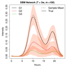
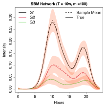
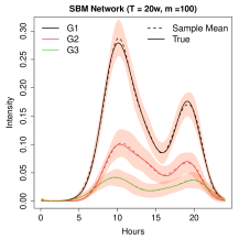
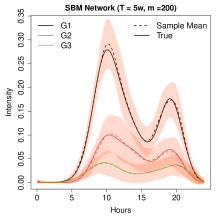
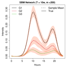
From Figure 4, we observe that the estimated background intensities become closer to the true background intensities as either $m$ or $T$ increases, which supports our theoretical findings in Theorems 2 (b) and 5 (a). Results for the Power-law network are similar and given in Section LABEL:sec:power-sim of the supplementary material. From Tables 2-3, we can see that when both $m$ and $T$ are small, the group memberships of a proportion of network nodes may be incorrectly estimated in both network settings. However, in all case scenarios, the GARs of the GNHP model are much better than those of the intensity-based K-means algorithm, which is used to provide initial membership estimates for the GNHP estimation, see Section A.2.1 of the supplementary material for details. As $m$ and/or $T$ increases, the GARs of the GNHP gradually approach $1$. This is consistent with our theoretical findings in Theorem 4. Consequently, as $m$ or $T$ increases, the estimation accuracy of the model parameters improves steadily and approaches that of the “Oracle” estimator. Overall, the simulation results support the estimation consistency of the proposed GNHP model when the group number $G$ is correctly specified.

Table 2: Estimation Accuracy of GNHP for SBM network when $G=G_{0}$.

$m=100$
		$\mu$ ($\times 10^{-3}$)	$\beta$($\times 10^{-3}$)	$\eta$ ($\times 10^{-3}$)	$\gamma$ ($\times 10^{-3}$)		$\phi$ ($\times 10^{-3}$)		GAR (s.e.)	GAR (s.e.)
$T$		GNHP (Oracle)	GNHP (Oracle)	GNHP (Oracle)	GNHP (Oracle)		GNHP (Oracle)		(GNHP with	(Intensity-based
	$g/g^{\prime}$	-	-	-	-	1	2	3	refinement)	K-means)
5$\omega$	1	340 (309)	16.3 (15.9)	199 (189)	212 (189)	29.1 (26)	45.3 (32.1)	29.6 (26.3)	95 (2.3)	53 (5.1)
	2	271 (249)	24.7 (22.4)	228 (211)	357 (336)	40.3 (39.3)	55.4 (51.1)	52.8 (48.9)
	3	192 (187)	26.5 (25.3)	431 (407)	183 (177)	21.7 (21.2)	34 (32.3)	29.1 (28.7)
10$\omega$	1	229 (228)	10.7 (10.7)	129 (127)	133 (127)	18.3 (17.9)	24.6 (23.2)	19.5 (18.3)	99 (0.93)	59 (4.2)
	2	184 (181)	15.4 (15.2)	148 (149)	237 (219)	28.2 (27.6)	35.7 (35.8)	34.4 (33.9)
	3	132 (132)	18 (18.4)	283 (284)	110 (109)	14.4 (14.4)	21.4 (21.9)	18.7 (18.5)
20$\omega$	1	165 (164)	7.31 (7.24)	92.7 (92.1)	93.5 (91)	13 (12.3)	15.4 (15.1)	12.3 (11.6)	100 (0.2)	64 (3.0)
	2	131 (129)	11.2 (11.7)	95.3 (95.6)	161 (164)	19.1 (19.8)	24.5 (24.3)	24 (24.2)
	3	95.8 (96.2)	12.5 (13.4)	207 (212)	78 (78.6)	10.3 (10.2)	15.8 (16)	13.6 (13.1)
40$\omega$	1	126 (126)	5.19 (5.35)	65.6 (63.7)	69.1 (67.2)	9.06 (9.32)	11.1 (11.2)	9.47 (9.66)	100 (0)	66 (2.5)
	2	93.8 (93.3)	7.77 (8.21)	66.5 (66.4)	110 (109)	13.3 (13.2)	16.7 (17.4)	15.8 (16.1)
	3	69 (69)	8.71 (8.64)	140 (143)	55.1 (54.5)	7.05 (6.96)	11.2 (10.2)	9.49 (9.32)
5$\omega$	1	272 (250)	12.2 (11.2)	148 (133)	218 (199)	36 (26)	29.9 (26.1)	25.3 (22.4)	94 (1.7)	49 (3.2)
	2	205 (182)	16.3 (14.3)	141 (129)	257 (236)	27.8 (27.3)	35.4 (32.7)	37.1 (34.7)
	3	152 (146)	18.2 (18.1)	307 (293)	144 (141)	18.3 (18)	28.4 (26.6)	20.5 (20)
10$\omega$	1	181 (179)	8.58 (8.4)	99.7 (98.5)	138 (136)	19.2 (18.1)	17.8 (17.4)	17.7 (17.5)	99 (0.72)	55 (3.4)
	2	136 (133)	10.5 (10.3)	95.3 (91.8)	167 (166)	19.6 (19.1)	23.9 (23.3)	24.7 (24.4)
	3	106 (106)	13.1 (13.3)	196 (190)	98.1 (101)	12.2 (12)	19.3 (19.5)	14.1 (14.2)
20$\omega$	1	133 (133)	5.65 (5.74)	69.5 (67.8)	98.5 (96.5)	12.7 (12.9)	12 (12.3)	11.3 (11.6)	100 (0.17)	64 (4.4)
	2	98.7 (97.7)	6.91 (7)	66.2 (68)	115 (115)	12.8 (13.1)	17.2 (17.1)	17.2 (17.4)
	3	77 (77.9)	8.81 (8.72)	144 (146)	64.6 (63.4)	8.98 (8.94)	13.7 (13.7)	10 (9.86)
40$\omega$	1	103 (103)	3.99 (4.01)	50.5 (50.1)	69.5 (69.3)	9.17 (9.21)	8.49 (8.44)	8 (7.91)	100 (0)	71 (4.4)
	2	72.3 (72.7)	5.01 (5.05)	47.4 (47.5)	82.2 (82.3)	9.37 (9.41)	12.2 (11.9)	12.2 (12.2)
	3	56.8 (56.9)	6.33 (6.32)	102 (101)	45.2 (44.7)	6.26 (6.24)	9.47 (9.33)	6.85 (6.77)

Table 3: Estimation Accuracy of GNHP for Power Law network when $G=G_{0}$.

RMSE TABLE, PL setting.
$m=100$
		$\mu$ ($\times 10^{-3}$)	$\beta$($\times 10^{-3}$)	$\eta$ ($\times 10^{-3}$)	$\gamma$ ($\times 10^{-3}$)		$\phi$ ($\times 10^{-3}$)		GAR (s.e.)	GAR (s.e.)
$T$		GNHP (Oracle)	GNHP (Oracle)	GNHP (Oracle)	GNHP (Oracle)		GNHP (Oracle)		(GNHP with	(Intensity-based
	$g/g^{\prime}$	-	-	-	-	1	2	3	refinement)	K-means)
5$\omega$	1	395 (349)	17.8 (15.5)	213 (193)	410 (362)	61 (50.4)	43.2 (38.8)	51.5 (46)	93 (2.8)	49 (4.3)
	2	340 (290)	23.5 (20.2)	213 (191)	449 (405)	50.4 (46.6)	55.5 (48.4)	74.4 (67.4)
	3	240 (231)	26.1 (25.4)	420 (388)	292 (283)	38 (37.8)	46.3 (42.4)	53.8 (51.8)
10$\omega$	1	249 (246)	12.4 (11.8)	140 (135)	237 (225)	32.3 (31.2)	28.8 (25.8)	31.6 (31.5)	99 (1.3)	55 (4.5)
	2	208 (202)	15 (14.3)	144 (137)	289 (272)	33.6 (32.7)	35.5 (33.8)	45.4 (45.3)
	3	161 (163)	17.2 (17)	296 (279)	153 (159)	26.5 (26)	26.1 (27.3)	34.3 (35.6)
20$\omega$	1	181 (179)	7.5 (8.13)	103 (96.9)	141 (151)	22.4 (22.4)	19.4 (19)	23.2 (22.6)	100 (0.31)	63 (5.6)
	2	149 (147)	9.89 (9.7)	92.2 (91.5)	208 (194)	22.9 (22.4)	22.5 (22.3)	34.7 (33.3)
	3	115 (117)	12.5 (12.1)	201 (197)	108 (106)	17.5 (17.8)	18.8 (19.4)	23.7 (24.8)
40$\omega$	1	133 (134)	5.71 (5.63)	70.5 (68.9)	119 (117)	16.2 (16.4)	13.5 (13.9)	16 (15)	100 (0.059)	74 (6.9)
	2	107 (106)	6.84 (6.89)	69 (67.7)	137 (137)	16.4 (16.7)	16.5 (16.4)	23.4 (23.8)
	3	83.1 (84.7)	9.29 (8.85)	143 (146)	72.9 (73)	12.6 (12.3)	14.2 (13.9)	17.3 (17.7)
5$\omega$	1	296 (254)	12.3 (9.92)	136 (118)	216 (191)	35.2 (25.5)	43.2 (32.1)	32.4 (30.6)	94 (1.9)	51 (3.6)
	2	281 (252)	17 (15)	164 (139)	331 (298)	32.1 (30.3)	45.7 (42.5)	56.2 (51)
	3	195 (188)	17.7 (17.2)	299 (287)	186 (181)	23 (22.5)	37.5 (37.6)	35.7 (34.1)
10$\omega$	1	191 (187)	7.25 (6.99)	85 (83.3)	137 (133)	20.5 (18.8)	26.2 (23.2)	21.3 (20.6)	99 (0.9)	59 (3.4)
	2	186 (181)	10.5 (10.4)	103 (97.4)	212 (202)	21.1 (20.9)	29.5 (29.3)	38.8 (37.5)
	3	139 (138)	12.9 (12.8)	214 (209)	117 (118)	16.1 (16.1)	24.8 (24.8)	23.9 (23.7)
20$\omega$	1	138 (137)	4.87 (4.96)	60.1 (58.9)	98.8 (100)	12.2 (12.1)	15.5 (15.9)	14.2 (14.4)	100 (0.2)	67 (3.2)
	2	128 (128)	7.43 (7.42)	68.5 (68.9)	146 (146)	14.4 (14.6)	21.7 (21.3)	26 (25.5)
	3	99.4 (99.1)	8.7 (8.61)	139 (141)	75.6 (76.7)	11.4 (11.1)	17.7 (18)	16.4 (16.4)
40$\omega$	1	110 (110)	3.23 (3.49)	39.4 (41.6)	82.8 (82.3)	9.34 (9.18)	11.2 (11.3)	10.4 (10.4)	100 (0.027)	75 (4.2)
	2	97 (95.3)	5.1 (5.11)	51.3 (49.6)	117 (110)	10.4 (10.5)	15.1 (15)	17.2 (18)
	3	72.6 (71.9)	6.09 (6.16)	91.5 (93.9)	52.5 (54)	7.56 (7.8)	11.7 (12.5)	12.2 (11.8)

5.2 Coverage Probability When $G=G_{0}$

We next investigate the quality of statistical inference for the GNHP model by evaluating the coverage probabilities of the $95\%$ confidence intervals for model parameters, derived through the limiting distribution given by Theorem 5 (b). For instance, the $95\%$ confidence interval for $\beta_{g}$ is given by CI${}_{\beta_{g}}^{(k)}=(\widehat{\beta}_{g}^{(k)}-1.96\widehat{\sigma}_{\beta_{g}}^{(k)},\widehat{\beta}_{g}^{(k)}+1.96\widehat{\sigma}_{\beta_{g}}^{(k)})$, where $\widehat{\sigma}_{\beta_{g}}^{(k)}$ is the square root of the corresponding diagonal entry of the estimated covariance matrix $\boldsymbol{\Sigma}_{\alpha}$. Empirical coverage probabilities based on $1000$ simulation runs are summarized in Table 4.

Table 4: Empirical coverage probabilities ($\%$) for the GNHP model parameters.

		SBM network												Power Law network
		$m=100$						$m=200$						$m=100$						$m=200$
$T$		$\beta_{g}$	$\eta_{g}$	$\gamma_{g}$		$\phi_{gg^{\prime}}$		$\beta_{g}$	$\eta_{g}$	$\gamma_{g}$		$\phi_{gg^{\prime}}$		$\beta_{g}$	$\eta_{g}$	$\gamma_{g}$		$\phi_{gg^{\prime}}$		$\beta_{g}$	$\eta_{g}$	$\gamma_{g}$		$\phi_{gg^{\prime}}$
	$g/g^{\prime}$	-	-	-	1	2	3	-	-	-	1	2	3	-	-	-	1	2	3	-	-	-	1	2	3
5$\omega$	1	93.8	93.4	91.5	92.1	85.5	91.3	93.3	94.9	91.8	82.2	91.8	93.5	94.4	95.2	93.1	84.8	92.6	84.4	89.2	93.9	90.8	86.8	85.3	92.6
	2	91.5	90.6	90.8	93.4	90.6	91.3	90.8	90	92.9	93.3	94.9	92.7	92.6	90.5	92.2	92.2	90.9	93.1	88.9	90.3	91.1	91.6	90.5	91.1
	3	95	92.1	93.3	94	92.5	94.4	94.9	93.3	93.1	94.9	94.1	93.7	92.2	95.2	95.7	92.6	91.3	92.2	94.7	94.2	92.1	94.7	91.8	91.6
10$\omega$	1	94.6	95.2	94.8	94.8	92.5	94.4	95.9	94.4	94.4	93	93.2	93.8	94.5	96.2	94.5	91.8	91.2	94	94.5	95.4	94.8	89	93.3	92
	2	96	93.7	94.2	91.5	93.5	92.9	94	93.4	94.6	96.5	96.1	94.8	97.3	95.6	94	94	91.2	96.7	95.1	93.6	93.6	92.7	96.3	93.3
	3	95.6	95.8	95.4	94.4	96.6	94.4	93.4	94.8	92.6	96.7	93.8	95.7	94	96.7	96.2	92.9	94	92.9	93.3	93.9	93.6	92.7	95.4	95.7
20$\omega$	1	96.6	93.8	94.2	93.4	95.8	96	95.5	95.1	95.5	95.5	95.7	94.6	95	95.6	95	92.5	93.1	95.6	96.6	95.2	92.2	95.2	94.2	95.6
	2	93.4	94.8	94.8	95.8	93.8	92.8	95.5	93.6	95.3	96.1	93.8	95.1	92.5	96.2	93.1	94.4	96.2	92.5	96.9	93.5	94.5	95.6	94.5	93.9
	3	94.4	93.8	95	93.6	94	93.8	95.1	93.1	95.7	94.2	91.9	94.9	97.5	92.5	91.9	95	95.6	95	91.8	96.6	95.9	95.6	95.6	93.5
40$\omega$	1	95	93.2	94.8	95.8	95.6	95	95.8	93.8	93.4	94	94.8	95.6	93.5	91.6	90.9	93.5	94.8	96.8	95.4	95.4	87.7	92.3	92.8	92.3
	2	93.6	95.2	94.4	94	95.6	96	94.2	94.2	94	94.6	95.6	94	92.2	92.9	91.6	92.2	97.4	93.5	95.4	91.3	90.8	92.8	94.9	94.9
	3	94.4	94.2	94.4	95.4	93	95.2	93.4	95.4	94	95.6	94.8	94.6	92.2	92.9	96.8	95.5	92.2	94.2	94.4	97.4	91.8	95.4	94.4	94.9

Table 4 shows that the coverage probabilities have some departure from the nominal $95\%$ when $m=100$ and $T=5\omega$ in both network settings, which is not surprising since on average only around 5% and 7% of group memberships are correctly estimated in these two settings. As $m$ and $T$ increase, the empirical coverage probabilities for almost all parameters approach the nominal level, which supports our theoretical findings in Theorem 5.

5.3 Estimation Accuracy with a Mis-specified $G$

When $G$ is mis-specified, we define PD${}_{\boldsymbol{\beta}}=\operatorname*{median}_{1\leq k\leq K}\big{\{}\frac{1}{m}\sum_{i=1}^{m}\big{|}\beta_{g_{i}^{0}}^{0}-\widehat{\beta}_{\widehat{g}_{i}^{(k)}}^{(k)}\big{|}\big{\}}$, and PD_η and PD_γ are similarly defined. For the estimated background intensities, we define PD${}_{\mu}=\operatorname*{median}_{1\leq k\leq K}\big{\{}\frac{1}{m}\sum_{i=1}^{m}\|\widehat{\mu}_{\widehat{g}_{i}^{(k)}}(t)-\mu_{g_{i}^{0}}^{0}(t)\|_{T}\big{\}}$, and for the network effects, we evaluate the estimation accuracy of the transition matrix $\mathbf{B}$ using PD_B = $\operatorname*{median}_{1\leq k\leq K}\Big{\{}\frac{1}{m}\sum_{i=1}^{m}\sum_{j=1}^{m}a_{ij}|\widehat{b}_{ij}^{(k)}-b_{ij}^{0}|\Big{\}}$. To identify the true number of groups, we use $\lambda_{mT}=({15T})^{-1}\left(\operatorname*{median}_{1\leq i\leq m}n_{i}\right)^{0.6}\bar{d}^{0.25}$ for the LIC in (16), and report the selection error rate as SR$(G)=K^{-1}\sum_{k=1}^{K}I(\widehat{G}^{(k)}=G)$, where $\widehat{G}^{(k)}$ maximizes the LIC in the $k$th simulation. To study the effect of the membership refinement algorithm in Section 4.4, we also compare the GARs with and without membership refinements. In the refinement step, we randomly sample $1,000$ $\boldsymbol{\psi}_{i}$’s to find the refined membership (20) if the candidate set size exceeds $1,000$.

Table 5: Estimation accuracy and selection rate of $G$ when $G$ is miss-specified.

		SBM network																Power Law network
		$m=100$								$m=200$								$m=100$								$m=200$
$T$	$G$	$\mu$	$\beta$	$\eta$	$\gamma$	$\mathbf{B}$	SR	GAR	GAR	$\mu$	$\beta$	$\eta$	$\gamma$	$\mathbf{B}$	SR	GAR	GAR	$\mu$	$\beta$	$\eta$	$\gamma$	$\mathbf{B}$	SR	GAR	GAR	$\mu$	$\beta$	$\eta$	$\gamma$	$\mathbf{B}$	SR	GAR	GAR
		$(\times 10^{-3})$					(%)	(%)	(w.o.r)	$(\times 10^{-3})$					(%)	(%)	(w.o.r)	$(\times 10^{-3})$					(%)	(%)	(w.o.r)	$(\times 10^{-3})$					(%)	(%)	(w.o.r)
5$\omega$	2	33.5	74.2	842	737	117	0	70.6(2.4)	70.5(2.2)	33.6	77	864	763	118	0	65.6(1.8)	64.7(2)	37	81.1	916	815	121	63	64.7(2.6)	64(2.6)	33.6	74.4	797	788	113	95	70.5(2.2)	69.2(2.9)
	3	19.8	30.2	389	301	51.5	100	94.6(2.3)	93.8(2.6)	16.7	24.9	319	285	49.1	100	94.6(1.6)	93.7(1.6)	24.4	34.4	424	442	72.4	37	92.8(2.9)	90.7(3.5)	19.6	27.7	310	336	56.6	5	93.8(1.9)	91.6(2.2)
	4	28.4	42.2	549	428	73.1	0	92.7(3.2)	91.1(3.4)	26.2	39.3	472	436	71.4	0	91.6(2.3)	91.1(2.4)	32.5	46.6	566	620	98.8	0	89.8(3.7)	86.6(4)	30.7	40.4	459	485	80.5	0	91.6(3)	89.3(2.8)
	5	33.8	46.1	614	490	83.8	0	91.4(3.2)	89.1(4)	30.5	46.4	540	535	84.2	0	90.5(3.1)	89.7(2.6)	38.4	52.7	630	751	115	0	88.7(3.9)	84.9(4.6)	36.9	45.9	524	569	94.8	0	90.6(3.1)	87.8(3)
	6	36.4	52.4	670	566	94.6	0	90.4(3.4)	87.2(4.9)	33.5	51.6	607	592	89.5	0	90.1(3)	88.6(3)	42.2	58.1	702	907	132	0	87.8(3.8)	83.7(5)	41	49.9	580	638	106	0	89.8(3.3)	87(2.9)
	oracle	14.8	17.8	235	218	31.9	-	- -	- -	11.4	13	171	182	25.6	-	- -	- -	16.7	19.8	233	299	43.9	-	- -	- -	13.5	13.7	161	212	30.1	-	- -	- -
10$\omega$	2	30.6	67.8	709	701	113	0	72.6(1.5)	72(1.9)	31.4	73.1	748	740	116	0	67.1(1.6)	66.3(1.9)	32.8	75	787	773	117	4	67.2(1.7)	66.5(2.2)	30.8	70	706	768	109	68	72.2(1.1)	71.5(1.7)
	3	11.4	14.5	188	152	25.7	100	99.2(0.91)	97.5(1.5)	9.36	11.7	135	147	21.9	100	99(0.7)	97(1)	13.3	15.9	205	235	36.1	96	98.5(1.2)	96(1.9)	11	12.3	149	156	27.5	32	98.6(0.84)	95.9(1.3)
	4	17	21.6	263	228	38.6	0	98.5(1.5)	97.1(1.6)	14.9	20.5	228	266	41	0	97.4(1.6)	96.4(1.4)	19.1	23.8	283	345	57.3	0	96.7(2.3)	94.7(2.3)	18	23	234	262	44.8	0	97.5(1.7)	95.3(1.9)
	5	20.5	24.8	308	275	46.8	0	98.2(1.4)	96.3(1.9)	18.7	24.5	268	279	46.6	0	97.4(1.7)	95.9(1.5)	22.4	27.4	332	399	66.8	0	96.5(2.2)	94.3(2.3)	22.9	25	274	312	56.8	0	96.9(1.9)	94.9(1.7)
	6	22.3	28.8	350	299	53	0	97.8(1.8)	95.5(2.3)	20.7	27.2	318	331	50.8	0	97.1(1.8)	95.8(1.5)	23.5	30.2	365	450	70.7	0	96.5(2.5)	93.5(2.7)	25.2	25.5	305	326	62.4	0	96.9(1.8)	94.3(2.2)
	oracle	10.7	13.6	178	135	22.5	-	- -	- -	8.35	9.55	113	129	17.8	-	- -	- -	11.7	13.4	173	213	30.3	-	- -	- -	9.9	9.06	116	130	21.3	-	- -	- -
20$\omega$	2	29.6	66.1	681	690	112	0	72.7(1.5)	71.6(2.7)	30.4	70.9	724	729	116	0	67.7(0.93)	66.9(1.9)	31.2	73.1	743	757	116	0	68(0.98)	67(2.2)	29.9	68.6	690	753	108	1	72.4(0.44)	71.7(2.5)
	3	7.9	9.48	116	109	15	99	99.9(0.26)	97.7(1.3)	6.18	6.75	91.6	95.7	12.5	100	99.9(0.2)	97.6(1.1)	8.67	9.72	118	155	21	100	99.9(0.31)	97.4(1.6)	7.28	6.71	82	101	15	99	99.9(0.25)	97.2(1.5)
	4	11	13.9	154	148	22.6	1	99.8(0.64)	97.8(1.4)	8.79	11.8	127	136	22.1	0	99.3(0.79)	97.9(1)	11.5	14.6	169	209	33.8	0	99.3(1.1)	97(1.7)	10.7	12.1	130	153	25.8	0	99.3(0.93)	97.1(1.3)
	5	12.6	16.2	178	168	27.9	0	99.8(0.48)	97.6(1.4)	11.5	13.6	161	184	26.8	0	99.3(0.85)	98(0.89)	13.4	17	195	225	39.1	0	99.2(1)	96.8(1.9)	14	13.7	153	185	32.1	0	99.2(0.93)	97.1(1.4)
	6	13.7	17.3	193	181	30.7	0	99.7(0.53)	97.2(1.4)	13.2	15.8	164	186	30.7	0	99.4(0.71)	97.5(0.99)	14.2	18.6	202	236	42.4	0	99.1(1.1)	96.3(1.7)	15.7	15.2	174	208	35.2	0	99.3(0.77)	96.9(1.2)
	oracle	7.87	9.35	115	108	14.8	-	- -	- -	6.09	6.44	90.6	92.5	12.4	-	- -	- -	8.6	9.69	116	153	20.6	-	- -	- -	7.22	6.59	77.4	98.9	14.7	-	- -	- -
40$\omega$	2	29.1	65	667	680	112	0	72.4(2.3)	71.6(3.5)	30	70.2	715	723	115	0	67.9(0.85)	67.1(2)	30.6	71.5	724	754	116	0	68.1(0.6)	67.9(1.4)	29.5	68.2	679	735	108	0	72.5(0.3)	72.4(0.87)
	3	5.82	6.93	81.7	73.8	10.9	99	100(0)	97.8(1.6)	4.49	4.43	61.3	60.6	8.73	100	100(0)	98.5(1.2)	6.33	6.52	80.3	108	15.6	100	100(0)	98.3(1.6)	5.73	4.47	53.4	79.4	10.3	100	100(0)	98.6(1.1)
	4	7.64	8.56	101	89.7	15.4	1	100(0.12)	98.2(1.3)	5.75	5.52	70.7	80.5	12.2	0	100(0.17)	98.7(0.94)	7.75	8.18	95	125	21.4	0	99.9(0.26)	98.5(1.3)	7.19	6.46	70.3	109	14.9	0	99.9(0.22)	98.2(1.3)
	5	8.93	10	114	97.8	18.7	0	100(0.11)	98(1.3)	7.29	7.61	103	105	16.4	0	99.9(0.18)	98.8(0.82)	8.42	9.82	117	144	24.7	0	100(0.25)	98.4(1.4)	8.94	7.17	81.8	123	19.3	0	100(0.17)	98.6(0.96)
	6	9.32	11.4	121	108	21.4	0	100(0.14)	98.1(1.2)	8.3	9.05	110	111	19.9	0	100(0.13)	98.6(0.93)	9.29	9.47	117	157	27.5	0	99.9(0.26)	98.4(1.1)	10	8.53	103	133	22.2	0	99.9(0.2)	98.1(1)
	oracle	5.83	6.91	80.8	73.7	10.8	-	- -	- -	4.51	4.46	62.3	60.9	8.71	-	- -	- -	6.27	6.52	81.1	109	15.6	-	- -	- -	5.73	4.32	53.6	81.7	10.5	-	- -	- -

Since the refinement step is rather time consuming, especially when $G$ is large, we only provide summary statistics based on $K=200$ simulation runs in Table 5, where we can see that even when $G$ is over-specified, the consistency result still holds. For instance, PD_β drops from approximately 42.2$\times 10^{-3}$ to 20.5$\times 10^{-3}$ as $(m,T)$ increases from $(100,5\omega)$ to $(200,10\omega)$ with $G=4$, which corroborates with the result in Theorem 2. When $G>3$, estimation errors are generally larger than those of the case with $G=G_{0}$, which is reasonable due to the additional estimation variability introduced by an overly large $G$. Furthermore, the proposed LIC can correctly select the true number of groups with a probability tending to $1$ as $(m,T)$ increases, which supports our conclusion of Theorem 3. Lastly, the GAR after the refinement tends to be slightly better than the GAR without the refinement, suggesting it is beneficial to perform membership refinement.

5.4 Computation Times

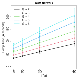
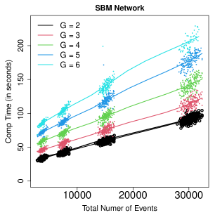
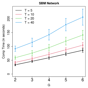
We now study the computation times of the proposed EM algorithm outlined in Section 3.3. For each initial membership estimate, we perform 100 Stochastic EM iterations, 50 EM iterations with fixed memberships, and then 50 EM iterations. Fixing $m=100$, computation times (in seconds) of this algorithm on a cluster of Intel Xeon Gold 6126 CPUs with 2.6 Ghz are summarized in Figure 5. We can see that the CPU time grows approximately linearly as $T$ and the total number of events increase. The CPU time grows slightly faster than linearly as $G$ increases since the number of parameters is of the order $Gn_{\rm kt}+3G+G^{2}$. Results are similar for the Power-law Network and are thus given in Section B.4 of the supplementary material. To increase the chance of finding the global optimal, for each simulation run, we use $50$ initial membership estimates following the intensity-based K-means algorithm (using different starting values, supplement with random membership estimates if less than 50 distinct membership estimates are generate). Since the computations with different initial values can be easily paralleled, the overall computation times of the proposed EM algorithm appears to be reasonable for practical use.

Figure 5: Computation times of the proposed EM algorithm in various settings.

6 EMPIRICAL STUDY: A SINA WEIBO DATASET

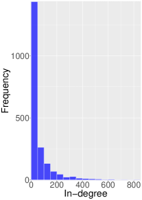
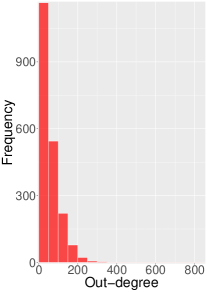
We apply the GNHP model to a dataset collected from Sina Weibo, the largest Twitter type social media in China, where we collect posting time stamps of $m=2,038$ users from January 1st to 15th, 2014, resulting in a $T=600$ hours. Details of the data collection process is given in Section B.5 of the Supplementary Material. Figure 6 gives two sample Weibo posts by James Cameron with posting times. The network adjacency matrix $A$ is constructed using the following-followee relationships among users, which gives the network density $\sum_{i,j}a_{ij}/m(m-1)=2.7\%$, suggesting a highly sparse network. Distributions of in-degrees and out-degrees of the network are given in Figure 6, where we can see that the in-degrees tend to be more skewed than the out-degrees. This phenomenon is typical for a social network platform, where a few influential users may have a large number of followers but most users do not follow too many other users.

Figure 6: Left panel: A snapshot of James Cameron’s Weibo posts; Middle panel: histogram of in-degrees; Right panel: histogram of out-degrees.

6.1 Model Estimation and Interpretation

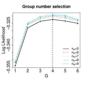
We approximate the background intensities of the GNHP model by periodic B-spline basis with $n_{\rm kt}=3,\cdots,10$ equally spaced knots between $[0,\omega]$ with $\omega=24$ (hours) and the triggering functions is of the form (3) with $b=5$ (hours). For better numerical stability, we put an upper bound $100$ on parameters $\eta_{g}$’s and $\gamma_{g}$’s. Using the EM algorithm proposed in Section 3.3 with $200$ initial membership and parameter estimates obtained from the algorithm in Section A.2 of the supplementary material, we first use the proposed LIC given in (16) to choose the number of latent groups with $\lambda_{mT}=({15T})^{-1}\left(\operatorname*{median}_{1\leq i\leq m}n_{i}\right)^{0.6}\bar{d}^{0.25}$. From Figure 7, we can see that the LICs have steep increases when $G$ changes from $1$ to $2$ for all choices of $n_{\rm kt}$’s, suggesting suitability to use a latent group structure to model the heterogeneity among network nodes. The optimal number of groups chosen by LIC is $G=4$ for all choices of $n_{\rm kt}$’s.

The next step is to choose the best $n_{\rm kt}$, for which we propose the following BIC type criterion:

$${\rm BIC}(n_{\rm kt},G)=-2mT\ell(\widehat{\underset{\widetilde{}}{\boldsymbol{\psi}}})+\log(mT/\omega)\times Gn_{\rm kt}T/\omega,$$ (23)

where $mT\ell(\widehat{\underset{\widetilde{}}{\boldsymbol{\psi}}})$ is the log-likelihood (10) evaluated at the MLE $\widehat{\underset{\widetilde{}}{\boldsymbol{\psi}}}$ given in (11).

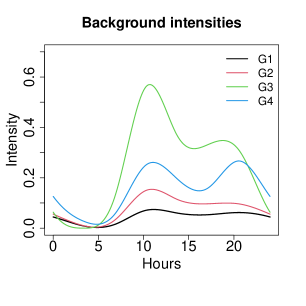
Heuristically, $T/\omega$ can be roughly interpreted as the number of weakly dependent replicates over time and $Gn_{\rm kt}T/\omega$ can be viewed as the total number of knots placed over $[0,T]$ and $G$ groups. Fixing $G=4$, Figure 7 shows that the minimum BIC value is achieved with $n_{\rm kt}=6$. The estimated background intensities using $n_{\rm kt}=6$ and $G=4$ are illustrated in Figure 7 and the resulting parameter estimates are summarized in Table 6.

Figure 7: Left panel: maximized log-likelihood of various $G$’s; Middle panel: LIC scores of various $G$’s; Right panel: estimated background intensities.

Table 6: Parameter estimates for Weibo data (p-values are given in the parentheses).

	Percent (%)	$\beta_{g}$	$\eta_{g}$	$\gamma_{g}$	$\phi_{gg^{\prime}}$
Group ($g/g^{\prime}$)	-	-	-	-	1	2	3	4
1	49.8	0.346 ($<$ 0.001)	9.69 ($<$ 0.001)	2.73 ($<$ 0.001)	0.0213 (0.0018)	0.0589 ($<$ 0.001)	0.00461 (0.0044)	0.0189 ($<$ 0.001)
2	28.2	0.343 ($<$ 0.001)	1.35 ($<$ 0.001)	2.49 ($<$ 0.001)	0.0474 ($<$ 0.001)	0.144 ($<$ 0.001)	0.0568 ($<$ 0.001)	0.00796 (0.24)
3	12.2	0.585 ($<$ 0.001)	0.603 ($<$ 0.001)	100 ($<$ 0.001)	0.00592 (0.55)	0.0344 ($<$ 0.001)	0.18 ($<$ 0.001)	0.00512 (0.53)
4	9.9	0.64 ($<$ 0.001)	7 ($<$ 0.001)	2.31 ($<$ 0.001)	0.0532 (0.1)	0.147 ($<$ 0.001)	0.0682 ($<$ 0.001)	0.181 ($<$ 0.001)

Figure 7 shows that all estimated background intensities have two peaks around 10:00 am and 8:00 pm, suggesting that users are more active around these times. Based on the estimated GNHP model and users’ information in the different groups, we summarize groups as following.

• Group 1 is largest group that includes $49.8\%$ of users, who have the lowest background intensity throughout the day. Judging from $\widehat{\phi}_{g1}$’s, users from this group have relatively low impact on users from other groups. This group also has the largest $\widehat{\eta}$ value, suggesting that the user’s past posts have the shortest time impacts on his/her future posting behavior.

• Group 2 include many users that are playing leading roles in various communities such as entertainment, business, education, and social sciences, who typically do not post very frequently throughout the day. This group has the second smallest $\hat{\eta}$ value, indicating that users’ past posts have a relatively long time effect. The estimated $\widehat{\phi}_{g2}$’s suggests that this group of users have the largest impacts on all groups except Group 3. Our subsequent analysis in Section 6.2 reveals that this group is the second most influential group.

• Group 3 mainly contains official accounts of some news outlets. Figure 7 shows that this group is the most active one on average, which is probably due to their mission to deliver information promptly. It has the smallest $\widehat{\eta}$, suggesting the longest temporal dependence on the posting histories. At the same time, it has an extremely large $\widehat{\gamma}$, which indicates that this group is very unlikely to be influenced by past posts from other groups. Although the estimated $\widehat{\phi}_{g3}$’s are not as large as those of Group 2, the largest background intensity of this group makes it the most influential group, as we shall demonstrate in Section 6.2.

• Group 4 consists of users who post quite frequently as suggested by Figure 7 but have rather limited impacts on other groups based on the estimated $\widehat{\phi}_{g4}$’s. It has a large $\widehat{\phi}_{42}=0.147$, indicating that users in this group are heavily influenced by users in Group 2.

6.2 Group Interaction and Influential User Analysis

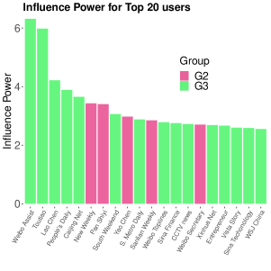
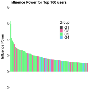
In social network analysis, identifying influential users is an important task, as it may help improve the efficiency of news propagation, product release, and promotional campaign launches. To identify the most influential users, we first define the influential power of the user $i$ as the sum of the $i$th column of $({\bf I}-\widehat{\bf B})^{-1}$, which is the Node-to-network influence given by Theorem 1. The bar plots of users with top 20 and 100 influential powers are illustrated in Figure 8, which shows that top 20 influential users only consist of members from Groups 2 and 3, with the latter group being the most influential one. This observation is further confirmed in the barplot of the top 100 influential users, where the majority of users are from Groups 2 and 3.

Figure 8: Barplot of top 20 and top 100 influential users.

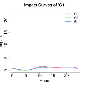
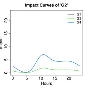
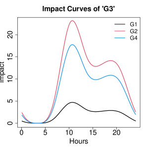
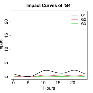
To shed more light on interactions among different groups, Figure 8 gives impact curves of each group on the other groups as defined in (5). As expected, both Groups 1 and 4 have rather limited impacts on other groups throughout the day. It appears that the most influential Group 3 has the largest impact on the Group 2, suggesting that users in Group 2 may have the greatest need for timely information provided by users in Group 3. Group 4 is impacted more heavily than Group 1 by Group 3, probably because users in Group 4 are relatively more active and hence can react to information from Group 1 more quickly. Lastly, the impact of Group 3 on Groups 1 and 4 are rather similar, an interesting phenomenon that may require a deeper look. Overall, the influence power plots and impact curve plots reveal some interesting interactive patterns among social network users, suggesting potential usefulness of the proposed GNHP model.

Finally, in Section B.5 of the supplementary material, we show the differences between groups obtained from GNHP and some simple alternative algorithms. More importantly, we remark that GNHP provides numerical quantification of user influence powers while others cannot.

7. DISCUSSION

We propose a group network Hawkes process (GNHP) that is suitable for analyzing the dynamic behavior patterns of heterogeneous users in a large network. The GNHP model extends the classical Hawkes model by utilizing the network structure and introduces a latent group structure to account for heterogeneity among network users. Theoretical properties are thoroughly investigated and a computationally efficient EM algorithm is proposed. The GNHP is highly interpretable, as we have demonstrated through an application to a Sina Weibo dataset.

The proposed model is suitable for abundant applications such as crime pattern analysis and financial risk management, as long as the network structure can be identified. Several research topics can be pursued for future studies. First, in many applications, the background intensities may be more complicated with multi-scale seasonalities such as daily, weekly, and annual seasonalities, in which case we can consider an additive background intensity $\mu(t)=\sum_{j=1}^{J}\mu_{g,j}(t-\lfloor t/\omega_{j}\rfloor{\omega_{j}})$ with an increasing $\omega_{1}<\omega_{2}<\cdots<\omega_{J}$ and each $\mu_{g,j}$ can be approximated by periodic splines. An alternative remedy is to introduce some time-dependent covariates such as “day of the week” or categorical variables such as “weekend or not?” and “holiday or not?”. Our theory can be easily modified for both extensions. One can further introduce user-specific covariates such as “age”, “gender” and “occupation” into the background intensities, but such extensions require non-trivial modifications of the current theory. Second, it will also be interesting to find a data-driven method to detect the period parameter $\omega$ if it is unknown. Next, while we have only considered one type of user behavior, it would be interesting to incorporate multi-type user behaviors into the model for analyzing data collected from a social network with more complicated structures. Finally, the network structure in the current framework is assumed to be known and fixed. It is also of great interest to extend the current model to be suitable for networks whose topological structures are evolving over time.

References

- Achab et al. (2018) Achab, M., Bacry, E., Gaiffas, S., Mastromatteo, I., and Muzy, J.-F. (2018), “Uncovering causality from multivariate Hawkes integrated cumulants,” Journal of Machine Learning Research, 18, 1–28.
- Amini et al. (2013) Amini, A. A., Chen, A., Bickel, P. J., and Levina, E. (2013), “Pseudo-likelihood methods for community detection in large sparse networks,” The Annals of Statistics, 41, 2097–2122.
- Bacry et al. (2020) Bacry, E., Bompaire, M., Gaïffas, S., and Muzy, J.-F. (2020), “Sparse and low-rank multivariate Hawkes processes,” Journal of Machine Learning Research, 21, 1–32.
- Bacry et al. (2013) Bacry, E., Delattre, S., Hoffmann, M., and Muzy, J.-F. (2013), “Modelling microstructure noise with mutually exciting point processes,” Quantitative Finance, 13, 65–77.
- Cai et al. (2020) Cai, B., Zhang, J., and Guan, Y. (2020), “Latent network structure learning from high dimensional multivariate point processes,” Working Paper.
- Chen and Hall (2013) Chen, F. and Hall, P. (2013), “Inference for a nonstationary self-exciting point process with an application in ultra-high frequency financial data modeling,” Journal of Applied Probability, 50, 1006–1024.
- Chen et al. (2017) Chen, S., Shojaie, A., Shea-Brown, E., and Witten, D. (2017), “The multivariate Hawkes process in high dimensions: Beyond mutual excitation,” arXiv preprint arXiv:1707.04928.
- Farajtabar et al. (2017) Farajtabar, M., Wang, Y., Gomez-Rodriguez, M., Li, S., and Zha, H. (2017), “COEVOLVE: A joint point process model for information diffusion and network evolution,” Journal of Machine Learning Research, 18, 1–49.
- Fleming and Harrington (2011) Fleming, T. R. and Harrington, D. P. (2011), Counting processes and survival analysis, vol. 169, John Wiley & Sons.
- Fox et al. (2016) Fox, E. W., Short, M. B., Schoenberg, F. P., Coronges, K. D., and Bertozzi, A. L. (2016), “Modeling e-mail networks and inferring leadership using self-exciting point processes,” Journal of the American Statistical Association, 111, 564–584.
- Halpin et al. (2013) Halpin, Peter, F., Boeck, D., and Paul (2013), “Modelling dyadic interaction with Hawkes processes,” Psychometrika, 78, 793–814.
- Hansen et al. (2015) Hansen, N. R., Reynaud-Bouret, P., Rivoirard, V., et al. (2015), “Lasso and probabilistic inequalities for multivariate point processes,” Bernoulli, 21, 83–143.
- Hawkes (1971) Hawkes, A. G. (1971), “Spectra of some self-exciting and mutually exciting point processes,” Biometrika, 58, 83–90.
- Hawkes and Oakes (1974) Hawkes, A. G. and Oakes, D. (1974), “A cluster process representation of a self-exciting process,” Journal of Applied Probability, 11, 493–503.
- Linderman and Adams (2014) Linderman, S. and Adams, R. (2014), “Discovering latent network structure in point process data,” in International Conference on Machine Learning, pp. 1413–1421.
- Liu et al. (2020) Liu, R., Shang, Z., Zhang, Y., and Zhou, Q. (2020), “Identification and estimation in panel models with overspecified number of groups,” Journal of Econometrics, 215, 574–590.
- Matias et al. (2018) Matias, C., Rebafka, T., and Villers, F. (2018), “A semiparametric extension of the stochastic block model for longitudinal networks,” Biometrika, 105, 665–680.
- Mohler et al. (2011) Mohler, G. O., Short, M. B., Brantingham, P. J., Schoenberg, F. P., and Tita, G. E. (2011), “Self-exciting point process modeling of crime,” Journal of the American Statistical Association, 106, 100–108.
- Ogata (1978) Ogata, Y. (1978), “The asymptotic behaviour of maximum likelihood estimators for stationary point processes,” Annals of the Institute of Statistical Mathematics, 30, 243–261.
- Ogata (1988) — (1988), “Statistical models for earthquake occurrences and residual analysis for point processes,” Journal of the American Statistical association, 83, 9–27.
- Rasmussen (2013) Rasmussen, J. G. (2013), “Bayesian inference for Hawkes processes,” Methodology and Computing in Applied Probability, 15, 623–642.
- Schütze et al. (2008) Schütze, H., Manning, C. D., and Raghavan, P. (2008), Introduction to information retrieval, vol. 39, Cambridge University Press Cambridge.
- Su et al. (2016) Su, L., Shi, Z., and Phillips, P. C. (2016), “Identifying latent structures in panel data,” Econometrica, 84, 2215–2264.
- Veen and Schoenberg (2008) Veen, A. and Schoenberg, F. P. (2008), “Estimation of space-time branching process models in seismology using an EM-type algorithm,” Journal of the American Statistical Association, 103, 614–624.
- Weng and Feng (2022) Weng, H. and Feng, Y. (2022), “Community detection with nodal information: likelihood and its variational approximation,” Stat, 11, e428.
- Xu et al. (2016) Xu, H., Farajtabar, M., and Zha, H. (2016), “Learning granger causality for hawkes processes,” in International Conference on Machine Learning, pp. 1717–1726.
- Yan and Sarkar (2021) Yan, B. and Sarkar, P. (2021), “Covariate regularized community detection in sparse graphs,” Journal of the American Statistical Association, 116, 734–745.
- Zarezade et al. (2018) Zarezade, A., De, A., Upadhyay, U., Rabiee, H. R., and Gomez-Rodriguez, M. (2018), “Steering social activity: a stochastic optimal control point of view,” Journal of Machine Learning Research, 18, 1–35.
- Zhang et al. (2021) Zhang, J., He, X., and Wang, J. (2021), “Directed community detection with network embedding,” Journal of the American Statistical Association, 1–11.
- Zhao et al. (2012) Zhao, Y., Levina, E., Zhu, J., et al. (2012), “Consistency of community detection in networks under degree-corrected stochastic block models,” The Annals of Statistics, 40, 2266–2292.
- Zhou et al. (2013) Zhou, K., Zha, H., and Song, L. (2013), “Learning social infectivity in sparse low-rank networks using multi-dimensional hawkes processes,” in Artificial Intelligence and Statistics, pp. 641–649.
- Zhou et al. (1998) Zhou, S., Shen, X., Wolfe, D., et al. (1998), “Local asymptotics for regression splines and confidence regions,” Annals of Statistics, 26, 1760–1782.
- Zhu et al. (2017) Zhu, X., Pan, R., Li, G., Liu, Y., and Wang, H. (2017), “Network Vector Autoregression,” The Annals of Statistics, 45, 1096–1123.
- Zhu et al. (2019) Zhu, X., Wang, W., Wang, H., and Härdle, W. K. (2019), “Network quantile autoregression,” Journal of econometrics, 212, 345–358.
- Zhu et al. (2022) Zhu, X., Xu, G., and Fan, J. (2022), “Simultaneous estimation and group identification for network vector autoregressive model with heterogeneous nodes,” arXiv preprint arXiv:2209.12229.