Avoiding Kernel Fixed Points:
Computing with ELU and GELU Infinite Networks

Abstract

Analysing and computing with Gaussian processes arising from infinitely wide neural networks has recently seen a resurgence in popularity. Despite this, many explicit covariance functions of networks with activation functions used in modern networks remain unknown. Furthermore, while the kernels of deep networks can be computed iteratively, theoretical understanding of deep kernels is lacking, particularly with respect to fixed-point dynamics. Firstly, we derive the covariance functions of multi-layer perceptrons (MLPs) with exponential linear units (ELU) and Gaussian error linear units (GELU) and evaluate the performance of the limiting Gaussian processes on some benchmarks. Secondly, and more generally, we analyse the fixed-point dynamics of iterated kernels corresponding to a broad range of activation functions. We find that unlike some previously studied neural network kernels, these new kernels exhibit non-trivial fixed-point dynamics which are mirrored in finite-width neural networks. The fixed point behaviour present in some networks explains a mechanism for implicit regularisation in overparameterised deep models. Our results relate to both the static iid parameter conjugate kernel and the dynamic neural tangent kernel constructions.

1 Background — Infinitely wide neural networks as Gaussian processes

Infinitely wide neural networks (NNs) and Gaussian processes (GPs) share an interesting connection (Neal 1995; Jacot, Gabriel, and Hongler 2018) which has only partially been explored. We begin by reviewing this connection. Readers familiar with this connection may skip to § 2. Consider a one-hidden layer network with independent parameters. Suppose each $i$th row of weights $\mathbf{W}_{i}$ together with the corresponding bias $B_{i}$ in the hidden layer has distribution $(\mathbf{W}_{i}^{\top},B_{i})^{\top}=\widetilde{\mathbf{W}_{i}}\sim\mathcal{N}\big{(}\mu,\Sigma)$, with $\Sigma\succ 0$ being a diagonal matrix having a unique “square root” $\Sigma^{(1/2)}$. Further, suppose the output layer parameter vector $\mathbf{V}=\frac{1}{\sqrt{n}}\mathbf{U}$ satisfies $\mathbf{U}\sim\mathcal{N}(\mathbf{0},\sigma_{w}^{2}I)$, where $n$ is the number of neurons in the hidden layer and the output bias satisfies $V_{b}\sim\mathcal{N}(0,\sigma^{2}_{b})$. The output evaluated at input $\mathbf{x}_{1}$ is $f(\mathbf{x}_{1})=\frac{1}{\sqrt{n}}\sum_{i=1}U_{i}\psi(\widetilde{\mathbf{W}}_{i}^{\top}\widetilde{\mathbf{x}}_{1})+V_{b}$, where $\psi$ is an activation function and $\widetilde{\mathbf{x}}_{1}=(\mathbf{x}_{1}^{\top},1)^{\top}$. The covariance between any two outputs is

$$\phantom{{}={}}k^{(1)}(\mathbf{x}_{1},\mathbf{x}_{2})$$

$$=\mathbb{E}\Big{[}\sum_{i=1}^{n}V_{i}\psi(\widetilde{\mathbf{W}}_{i}^{\top}\widetilde{\mathbf{x}}_{1})\sum_{j=1}^{n}V_{j}\psi(\widetilde{\mathbf{W}}_{j}^{\top}\widetilde{\mathbf{x}}_{2})\Big{]}{+}\sigma_{b}^{2}$$

$$=\sigma_{w}^{2}\mathbb{E}\Big{[}\psi(\widetilde{\mathbf{W}}_{1}^{\top}\widetilde{\mathbf{x}}_{1})\psi(\widetilde{\mathbf{W}}_{1}^{\top}\widetilde{\mathbf{x}}_{2})\Big{]}+\sigma_{b}^{2}.$$

The expectation over $d+1$ random variables reduces to an expectation over $2$ random variables, $\widetilde{\mathbf{W}}_{1}^{\top}\widetilde{\mathbf{x}}_{1}$ and $\widetilde{\mathbf{W}}_{1}^{\top}\widetilde{\mathbf{x}}_{2}$. The joint distribution of these two random variables is a bivariate Gaussian. The mean of each component is zero, and the variance is $\|\Sigma^{(1/2)}\widetilde{\mathbf{x}}_{i}\|^{2}$, where $\|\cdot\|$ denotes the Euclidean norm. The covariance is $\|\Sigma^{(1/2)}\widetilde{\mathbf{x}}_{1}\|\|\Sigma^{(1/2)}\widetilde{\mathbf{x}}_{2}\|\cos\theta$, where $\theta$ is the angle between $\Sigma^{(1/2)}\widetilde{\mathbf{x}}_{1}$ and $\Sigma^{(1/2)}\widetilde{\mathbf{x}}_{2}$. Therefore, the expectation in terms of $\mathbf{Z}\sim\mathcal{N}(\mathbf{0},S)$ is

$$k^{(1)}(\mathbf{x}_{1},\mathbf{x}_{2})=\sigma_{w}^{2}\mathbb{E}\Big{[} \psi\big{(}s_{1}Z_{1}+\widetilde{\mu}_{1}\big{)}\psi\big{(}s_{2}Z_{2}+\widetilde{\mu}_{2}\big{)}\Big{]}+\sigma_{b}^{2},$$ (1)

where $S$ has diagonals $1$ and off-diagonals $\cos\theta$, $s_{i}=\|\Sigma^{(1/2)}\widetilde{\mathbf{x}}_{i}\|$ and $\widetilde{\mu}_{i}=\bm{\mu}^{\top}\widetilde{\mathbf{x}}_{i}$.

Definition 1.

We call (1) the kernel. We call $\cos\theta^{(1)}=\frac{k^{(1)}(\mathbf{x}_{1},\mathbf{x}_{2})}{\sqrt{k^{(1)}(\mathbf{x}_{1},\mathbf{x}_{1})k^{(1)}(\mathbf{x}_{2},\mathbf{x}_{2})}}$ the normalised kernel.

The above NN converges to a GP as $n\to\infty$ under mild conditions on the input and activation function $\psi$ (Neal 1995). Since $f(\mathbf{x}_{1})$ is a sum of independent random variables scaling as $n^{-1/2}$, it converges to a Gaussian random variable with zero mean as $n\to\infty$. More generally, any fixed collection of $N$ evaluations of $f$, $\{f(\mathbf{x}_{i})\}_{i=1}^{N}$ converges to an $N$-dimensional $\mathbf{0}$-mean Gaussian as $n\to\infty$.

Analytical and closed-form covariance functions (1) are available for specific choices of $\psi$ (Le Roux and Bengio 2007; Tsuchida, Roosta, and Gallagher 2018; Tsuchida, Roosta, and Gallagher 2019a; Pearce et al. 2019; Tsuchida, Roosta, and Gallagher 2019b), although some of these require $\bm{\mu}=0$. Most notably, the kernel is known for historically relevant activation functions $\psi(z)=\text{erf}(z)$, RBF networks (Williams 1997) and for the more modern ReLU activation, $\psi(z)=\max(0,z)$ (Cho and Saul 2009). More recently Meronen, Irwanto, and Solin (2020) solved the inverse problem, finding $\psi$ that recovers the Matérn class of covariance functions. Once the form of (1) is known, the kernel of deep networks can be evaluated in the case where $\Sigma=\text{diag}(\sigma_{w}^{2},...,\sigma_{w}^{2},\sigma_{b}^{2})$ and ${\bm{\mu}=\bm{0}}$ (Matthews et al. 2018; Lee et al. 2018; Yang 2019b, a). The case where $\bm{\mu}\neq 0$ can also be handled (Tsuchida, Roosta, and Gallagher 2019b), but we focus on $\bm{\mu}=0$ in this work. The kernel in layer $l+1$ can be found iteratively as a function of the kernel in layer $l$,

$$k^{(l+1)}(\mathbf{x}_{1},\mathbf{x}_{2}) =\sigma_{w}^{2}\mathbb{E}\Big{[}\psi\big{(}s_{1}^{(l)}Z_{1}^{(l)}\big{)}\psi\big{(}s_{2}^{(l)}Z_{2}^{(l)}\big{)}\Big{]}+\sigma_{b}^{2},$$

$$\begin{bmatrix}Z_{1}^{(l)}\\ Z^{(l)}_{2}\end{bmatrix} \sim\mathcal{N}\Bigg{(}\mathbf{0},\begin{bmatrix}1&\cos\theta^{(l)}\\ \cos\theta^{(l)}&1\end{bmatrix}\Bigg{)},$$ (2)

where $\cos\theta^{(l)}$ is the normalised kernel in layer $l$, and $s_{i}^{(l)}=\sqrt{k^{(l)}(\mathbf{x}_{i},\mathbf{x}_{i})}$.

Definition 2.

We call $k^{(l)}$ in (2) the kernel in layer $l$. We call $\cos\theta^{(l)}=\frac{k^{(l)}(\mathbf{x}_{1},\mathbf{x}_{2})}{\sqrt{k^{(l)}(\mathbf{x}_{1},\mathbf{x}_{1})k^{(l)}(\mathbf{x}_{2},\mathbf{x}_{2})}}$ the normalised kernel in layer $l$.

A generalisation of iid weight priors to partially exchangeable weight priors is also available (Tsuchida, Roosta, and Gallagher 2019b), resulting in a GP with an additional layer of inference over the hyperparameters $\bm{\mu}$ and $\Sigma$. Convergence to GPs also occurs for other NN architectures such as convolutional architectures (Garriga-Alonso, Rasmussen, and Aitchison 2018; Novak et al. 2019) and general compositions of recurrent, graph convolution, pooling, skip connection, attention and normalisation layers (Yang 2019b, a). When an MLP is trained under a continuous-time analogue of gradient descent, the limiting output is still a GP (Jacot, Gabriel, and Hongler 2018). The dynamics and associated covariance of the GP depends on the neural tangent kernel (NTK) $T^{(l)}$, which in addition to the iterations (2), is given by

$$T^{(1)}(\mathbf{x}_{1},\mathbf{x}_{2}) =k^{(1)}(\mathbf{x}_{1},\mathbf{x}_{2})$$

$$\dot{k}^{(l+1)}(\mathbf{x}_{1},\mathbf{x}_{2}) =\sigma_{w}^{2}\mathbb{E}\Big{[}\psi^{\prime}(s_{1}Z^{(l)}_{1})\psi^{\prime}(s_{2}Z^{(l)}_{2})\Big{]},$$

$$T^{(l+1)}(\mathbf{x}_{1},\mathbf{x}_{2}) =T^{(l)}(\mathbf{x}_{1},\mathbf{x}_{2})\dot{k}^{(l+1)}(\mathbf{x}_{1},\mathbf{x}_{2})$$

$$\phantom{{}={}}+k^{(l+1)}(\mathbf{x}_{1},\mathbf{x}_{2}).$$ (3)

2 Contributions and motivation

Figure 1: Illustration of simplicity bias due to kernel fixed points. Training data $\mathbf{x}\in\mathbb{R}^{2}$ is uniformly sampled on the unit disc at heading $\gamma$. Curves show the posterior mean of a GP regression model on $y=\sin(\gamma)+\epsilon$ with known additive noise variance. $\sigma_{w}$ is chosen according to Figure 3. Colours move from purple to yellow as depth increases from $1$ to $64$. (Left) GELU without unique kernel fixed point leading to overfitting (Right) ReLU with unique kernel fixed point leading to underfitting. More examples in Appendix M.

This paper contains two main contributions. We:

1. Derive kernels for GELU and ELU activations (defined below) and verify our results numerically. We implement GPs with different NN kernels on some benchmarks.

2. Study the fixed point dynamics of the kernel when $\psi$ is bounded by the absolute value of a polynomial. We find sufficient conditions for the existence of a unique kernel fixed point. We show theoretically and empirically that unlike the kernel corresponding to ReLU $\psi$, the new kernels are able to avoid unique fixed points. These conditions apply to both the iid prior (Neal 1995) and dynamic NTK (Jacot, Gabriel, and Hongler 2018) cases. This fixed point behaviour can be used to explain a simplicity bias in deep NN. More surprisingly, we find theoretically that the NTK dynamic which approximates gradient descent preserves this simplicity bias.

2.1 Motivation for studying fixed points

Viewing NNs through the arguably idealised lens of GPs has some surprisingly non-intuitive practical implications. One important open problem is in explaining the empirical observation that some overparameterised NNs do not overfit, even when trained without explicit regularisation (Zhang et al. 2017). Tsuchida, Roosta, and Gallagher (2019b) show empirically that samples from the limiting prior of deep MLPs with zero-mean parameters and LReLU activations are approximately constant on the unit hypersphere. Valle-Pérez, Camargo, and Louis (2019) argue that deep NNs with ReLU activations exhibit a “simplicity bias”, in that randomly initialised NNs implementing Boolean functions are likely to be simple. Yang and Salman (2019) explain this simplicity bias through a spectral decomposition of the limiting kenel, showing that most of its mass is concentrated around the constant eigenfunction, even when accounting for training using gradient descent under the NTK (Jacot, Gabriel, and Hongler 2018). Yang and Salman (2019) are clear to separate the case of ReLU activations, which do result in kernels having peaked spectral mass and exhibiting a simplicity bias, from ERF activations which do not.

$$k(\mathbf{x}_{1},\mathbf{x}_{2})=$$

$$\sigma_{b}^{2}+\sigma_{w}^{2}\Bigg{(}\frac{s_{1}s_{2}}{4}\cos\theta+\frac{s_{1}^{2}s_{2}^{2}}{2\pi}\Bigg{[}\frac{\frac{1}{2}(\cos(2\theta)+3)+s_{1}^{2}+s_{2}^{2}+s_{1}^{2}s_{2}^{2}\sin^{2}\theta}{(1+s_{1}^{2})(1+s_{2}^{2})\sqrt{1+s_{1}^{2}+s_{2}^{2}+s_{1}^{2}s_{2}^{2}\sin^{2}\theta}}+\frac{\cos\theta}{s_{1}s_{2}}\tan^{-1}\Bigg{(}\frac{\cos\theta s_{1}s_{2}}{\sqrt{1+s_{1}^{2}+s_{2}^{2}+s_{1}^{2}s_{2}^{2}\sin^{2}\theta}}\Bigg{)}\Bigg{]}\Bigg{)}$$

Figure 2: The GELU kernel. Plots show the normalised kernels in layer $l$ as a function of the angle $\theta^{(0)}$ between the inputs for MLPs of increasing depth when $\Sigma=\text{diag}(\sigma_{w}^{2},...,\sigma_{w}^{2},0)$ and $\|\mathbf{x}_{i}\|$ is constant for all $i$. Values of $\sigma_{w}$ are chosen to preserve the expected square norm $\|\mathbf{x}\|^{2}$ (see § 4.1). Solid curve shows infinitely wide limit, and dots show samples from a network with $2$ inputs and $3000$ neurons in each layer. Each dot corresponds to an $\mathbf{x}_{1}$ and $\mathbf{x}_{2}$ generated through a random rotation of $(1,0)^{\top}$ and $(\cos\theta^{(0)},\sin\theta^{(0)})^{\top}$. The random rotation is found through a QR decomposition of a matrix containing entries sampled independently from $\mathcal{U}[0,1]$. (Left) $\|\mathbf{x}\|=0.5$, $\sigma_{w}=1.59$ (Middle) $\|\mathbf{x}\|=1$, $\sigma_{w}=1.47$. (Right) $\|\mathbf{x}\|=5$, $\sigma_{w}=1.42$.

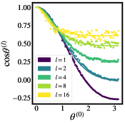
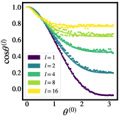
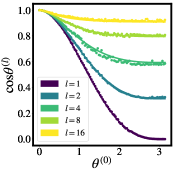
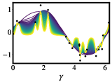
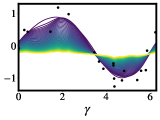
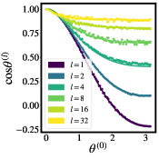
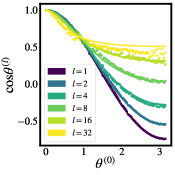
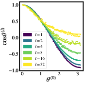
Our motivation for studying fixed points is in a similar spirit to the work above. For LReLU networks, we observe a so called kernel fixed point. An infinitely deep LReLU network is degenerate, and therefore over-regularised, in that all functions in the prior are constant over inputs on any hypersphere. Therefore, increasingly deep kernels represent a strict and potentially undesirable prior. On the other hand, kernels corresponding to GELU and ELU activation functions do not exhibit unique fixed points, and are therefore less biased towards simple functions. Just as traditional regularisation frameworks allow practitioners to control the bias-variance trade-off, in our framework, the activation function represents a similar choice. A deep ReLU network contains a higher degree of implicit regularisation than a deep GELU network. An illustration of this effect is shown in Figure 1. Even more surprisingly, our analysis extends to the NTK.

2.2 Recently introduced activation functions

The increased volume of gradient-based deep learning research has seen the introduction of new popular activation functions. Notably these include the exponential linear unit (ELU) (Clevert, Unterthiner, and Hochreiter 2016), the Gaussian error linear unit (GELU) (Hendrycks and Gimpel 2016) and the Swish (Ramachandran, Zoph, and Le 2017; Elfwing, Uchibe, and Doya 2018). The GELU and ELU are

$$\psi(z)=z\Phi(z)\text{ and }\psi(z) =\Theta(z)z+\Theta(-z)(e^{z}-1),$$

respectively, where $\Phi$ denotes the CDF of the standard Gaussian and $\Theta$ denotes the Heaviside step function.

Many state-of-the-art models use GELU (Radford et al. 2018; Devlin et al. 2019) or swish activations (Chua et al. 2018). However, even when critically evaluating empirical evidence, it is difficult to determine whether certain activation functions are a better choice for a given problem, let alone separate the activation function expressivity from the ability of optimisers to find good solutions. Analysing activation functions through the lens of GPs allows one to visualise the function space in isolation of the ability of the optimiser to find good solutions, and reveals interesting implicit regularisation structure in the infinitely wide setting.

2.3 Model selection

The choice of activation function in an NN can be framed as a model selection problem, and as such shares similarities with choosing other model hyperparameters. Take the case of choosing the L2 ridge-regularisation parameter as an example. One could apply n-fold cross-validation, with an implicit understanding that this parameter penalises model complexity as measured through the norm in an RKHS. Alternatively, a Bayesian might interpret the L2 weighting as the precision of a Gaussian prior, and optimise the marginal likelihood with respect to this weighting. A more pure Bayesian might put a prior over the regularisation (or precision) parameter and marginalise over these models. Common to all these approaches is (a) an intuition based on theory of what the parameter does and (b) a practical methodology for dealing with the parameter. In this paper we provide (a), and leave it to the practitioner to decide on (b) based on their philosophy and/or apparatus. Our work shows that GELU and ELU activations can avoid a regularisation mechanism that grows with depth that is always implicit in ReLU activations.

We stress that the new kernels and the fixed point mechanisms are neither “good” nor “bad” in isolation. The new models should be evaluated according to model selection criteria in their given application, and the fixed point mechanisms describe a regularisation implicit in some kernels.

Figure 3: As in Figure 2, but with ELU $\psi$. (Left-Right) $(\|\mathbf{x}\|,\sigma_{w})=(5,1.40)$, $(1,1.26)$, $(0.5,1.17)$.

3 New kernels

Proposition 3.

When $\psi$ is the GELU and $\bm{\mu}=0$, the kernel (1) is given by the equation in Figure 2.

The derivation is in the same spirit as Williams (1997); we introduce dummy parameters $\beta_{1}$ and $\beta_{2}$ in the argument of $\Phi$, differentiate with respect to $\beta_{1}$ and $\beta_{2}$ to obtain a PDE, then solve the PDE and evaluate the solution at $\beta_{1}=\beta_{2}=1$. Complete working is given in Appendix A. It is plausible that our method of derivation extends to the case $\bm{\mu}\neq 0$, although the calculations and resulting expression become more complicated. Even with $\bm{\mu}=0$, this kernel has some interesting properties that we discuss in § 4. Interestingly, unlike the ELU kernel with $\bm{\mu}=0$, the GELU kernel does not contain any hard-to-compute special functions, only some (inverse) trigonometric functions.

Our expression for the ELU kernel is lengthy and we do not assemble it in the main text, but provide a visualisation in the form of Figure 3.

Proposition 4.

When $\psi$ is the ELU, the kernel (1) has an analytical expression implemented in softwarefootnote:software in terms of the univariate and bivariate normal CDFs.

Complete working is given in Appendix B. Unfortunately, the ELU kernel involves exponentiating arguments involving $s_{1}$ and $s_{2}$. This can lead to numerical instability in GP regression when many data points are involved. Despite this, having an analytical expression still allows us to gain insights into finite width networks, as we shall see in § 4.

The scaled exponential linear unit (SELU) (Klambauer et al. 2017) is a slightly modified version of the ELU which introduces two scaling parameters: one applied over the entire domain and one over the negative domain. Our analysis for the ELU also handles the SELU (see Appendix B). Klambauer et al. (2017) motivates the SELU by showing that it is able avoid the exploding and vanishing gradient problem by carefully selecting the value of the scaling parameters. An entirely distinct problem is to analyse the correlations between signals in the network. Fixed points in signal norms are desirable to maintain the scale of signals as they propagate through the network. Fixed points in signal correlations can be undesirable as they force unrelated inputs to have similar feature representations in deep layers of the network. While Klambauer et al. (2017) is concerned with obtaining fixed points of signal norms (i.e. our § 4.1), it does not relate to fixed points of signal correlations (i.e. our § 4.2).

4 Fixed point analysis

In this section, we first analyse the conditions under which the expected squared norm of the signals in each layer are preserved as the signal propagates through the network for a different choices of the activation function (§ 4.1). In such a situation, the expected squared norm remains at a fixed point as it passes through the network. Then, more generally, we analyse conditions under which the expected squared norm of any two signals and the cosine angle between them approaches a constant as depth increases (i.e., when the kernel has a fixed point). We are especially interested in the case where the cosine angle between the signals converges to a unique fixed point (§ 4.2). Finally, we relate the existence of a unique fixed point to a degenerate, underfitting property of very deep infinitely wide MLPs (§ 4.3).

For § 4, 5 and 6, we suppose all the weights have the same variance, and so do all the biases; the first $d$ diagonals of the diagonal matrix $\Sigma$ are $\sigma_{w}^{2}$, and the last diagonal is $\sigma_{b}^{2}$.

4.1 Warm-up — norm preservation

A useful application of the kernel in finite-width iid-initialised networks is to track the expected squared norm of the signals in each layer as the depth of the network increases. This is used in initialisation to avoid exploding or vanishing signals when using gradient optimisers.

The expected norm squared of the signal in the first hidden layer is $(k^{(1)}(\mathbf{x}_{1},\mathbf{x}_{1})-\sigma_{b}^{2})/\sigma_{w}^{2}$. For the squared norm of the signal in the hidden layer to be the same as the squared norm of the input, we set $\|\widetilde{\mathbf{x}}_{1}\|^{2}=(k^{(1)}(\mathbf{x}_{1},\mathbf{x}_{1})-\sigma_{b}^{2})/\sigma_{w}^{2}$. We may then solve this condition to find the hyperparameter values that preserve input norms. For example, using the kernel corresponding to ReLU (Cho and Saul 2009), one obtains He initialisation (He et al. 2015), that $\sigma_{w}=\sqrt{2}$, where $\Sigma^{1/2}=\text{diag}(\sigma_{w},...,\sigma_{w},0)^{\top}$.

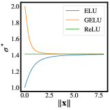
The analogue for GELU is more involved since no single $\sigma_{w}$ preserves the expected square norms of all inputs. Setting $\sigma_{b}=0$, $k(\mathbf{x},\mathbf{x})/\sigma_{w}^{2}=\|\mathbf{x}\|^{2}$ and $s_{1}=s_{2}=\sigma_{w}\|\mathbf{x}\|$ in the equation in Figure 2, we find a root $\sigma^{*}(\|\mathbf{x}\|)$ of

$$g_{\|\mathbf{x}\|}(\sigma) =\frac{\sigma^{4}\|\mathbf{x}\|^{2}}{\pi(\sigma^{2}\|\mathbf{x}\|^{2}+1)\sqrt{2\sigma^{2}\|\mathbf{x}\|^{2}+1}}+$$

$$\phantom{{}={}}\frac{\sigma^{2}}{4}\Big{(}1+\frac{2}{\pi}\sin^{-1}\frac{\sigma^{2}\|\mathbf{x}\|^{2}}{1+\sigma^{2}\|\mathbf{x}\|^{2}}\Big{)}-1,$$

numerically. Figure 4 shows a plot of $\sigma^{*}(\|\mathbf{x}\|)$ as $\|\mathbf{x}\|$ varies. The root of the limit of $g_{\|\mathbf{x}\|}(\sigma)$ as $\|\mathbf{x}\|\to\infty$ is $\sqrt{2}$, which recovers He initialisation. This implies that when data has large norms (such as images or audio files), He initialisation is suitable. The same procedure can be carried out for the ELU kernel as shown in Figure 4. This procedure may be viewed as a warm-up handling the special case of $\mathbf{x}_{1}=\mathbf{x}_{2}$ for our general fixed point analysis.

4.2 General fixed point analysis

Figure 4: (Left) Values $\sigma^{*}$ that preserve the layer-wise expected square norm of $\|\mathbf{x}\|$ in MLPs with GELU, ELU and ReLU activations. (Middle) lower bound of $\lambda_{3}$ for GELU (Right) $\lambda_{3}$ for ELU. If $\lambda_{3}\leq 1$ on $\theta\in(0,\pi)$, a unique fixed point exists.

Let $\mathcal{S}\subseteq[0,\infty)\times[0,\infty)\times[-1,1]$. In the infinitely wide limit, we may view each layer as updating a state $(s_{1}^{2},s_{2}^{2},\cos\theta)\in\mathcal{S}$ containing the expected square norms and the cosine angle between the signals in the hidden layers through a function $\mathbf{g}:\mathcal{S}\to\mathcal{S}$. Let $(G_{1},G_{2})^{\top}\sim\mathcal{N}(\mathbf{0},I)$. We study the fixed-point dynamics of the iterated map $\mathbf{g}$ having components

$$g_{1}(s_{1}^{2},s_{2}^{2},\rho) =\sigma_{w}^{2}\mathbb{E}\big{[}\psi^{2}(s_{1}G_{1})\big{]}+\sigma_{b}^{2},$$

$$g_{2}(s_{1}^{2},s_{2}^{2},\rho) =\sigma_{w}^{2}\mathbb{E}\big{[}\psi^{2}(s_{2}G_{2})\big{]}+\sigma_{b}^{2}$$

$$g_{3}(s_{1}^{2},s_{2}^{2},\rho) =$$

$$\frac{\mathbb{E}\Big{[}\sigma_{w}^{2}\psi(s_{1}G_{1})\psi\big{(}s_{2}(G_{1}\rho+G_{2}\sqrt{1-\rho^{2}})\big{)}+\sigma_{b}^{2}\Big{]}}{\sqrt{g_{1}(s_{1}^{2},s_{2}^{2},\rho)g_{2}(s_{1}^{2},s_{2}^{2},\rho)}},$$ (4)

which track the expected square norms (after a linear transformation involving $\sigma_{w}^{2}$ and $\sigma_{b}^{2}$) and normalised kernel as the signals propogate through the layers. By inspection, $g_{3}$ (but not necessarily $\mathbf{g}$) always has an uncountable set of fixed points at $\rho=1$ along $s_{1}=s_{2}$. Banach’s fixed point theorem says that if $\mathbf{g}$ is a contraction mapping on a closed set, then $\mathbf{g}$ has a unique fixed point on that set (Agarwal, Meehan, and O’regan 2001). In a slightly different setting, Hasselblatt and Katok (2003, Theorem 2.2.16) allows some open sets.

Theorem 5.

Let $D\mathbf{g}$ denote the Jacobian of $\mathbf{g}$ and $d^{\prime}$ denote the metric induced by a norm with induced matrix norm $\|\cdot\|^{\prime}$. If $C\subset\mathbb{R}^{m}$ is an open strictly convex set, $\overline{C}$ is its closure, $\mathbf{g}:\overline{C}\to\overline{C}$ differentiable on $C$ and continuous on $\overline{C}$ with $\|D\mathbf{g}\|^{\prime}\leq\lambda<1$ on $C$, then $\mathbf{g}$ has a unique fixed point $\mathbf{c}_{0}\in\overline{C}$ and $d^{\prime}\big{(}\mathbf{g}^{L}(\mathbf{c}),\mathbf{c}_{0}\big{)}\leq\lambda^{L}d^{\prime}(\mathbf{c},\mathbf{c}_{0})$ for every $\mathbf{c}\in\overline{C}$.

We therefore consider the eigenvalues of the Jacobian, proving the following in Appendix C.

Theorem 6.

Let $\mathbf{g}$ be as in (4), and suppose the absolute value of $\psi$ is bounded by a polynomial. Let $(Z_{1},Z_{2})\sim\mathcal{N}(\mathbf{0},S)$ with covariance $\rho=\cos\theta$ and unit variances. Then for $\rho\in(-1,1)$ $0<s_{1},s_{2}$, the (unordered) eigenvalues of the Jacobian of $\mathbf{g}$ are

$$\lambda_{1}:=\frac{\partial g_{1}}{\partial s_{1}^{2}} =\sigma_{w}^{2}\mathbb{E}\Big{[}\big{(}Z_{1}^{2}-1\big{)}\psi^{2}(s_{1}Z_{1})\Big{]}/(2s_{1}^{2}),$$

$$\lambda_{2}:=\frac{\partial g_{2}}{\partial s_{2}^{2}} =\sigma_{w}^{2}\mathbb{E}\Big{[}\big{(}Z_{2}^{2}-1\big{)}\psi^{2}(s_{2}Z_{2})\Big{]}/(2s_{2}^{2}),\quad\text{and}$$

$$\lambda_{3}:=\frac{\partial g_{3}}{\partial\rho} =\frac{\sigma_{w}^{2}s_{1}s_{2}}{\sqrt{g_{1}g_{2}}}\mathbb{E}\big{[}\psi^{\prime}(s_{1}Z_{1})\psi^{\prime}(s_{2}Z_{2})\big{]},$$

provided the right hand terms are finite, where $\psi^{\prime}$ is the distributional derivative of $\psi$.

Our result does not include $\rho\in\{-1,1\}$. With the additional assumption that $\psi$ is continuous almost everywhere, the expression for $\lambda_{3}$ is valid on the closed interval $\rho\in[-1,1]$, as shown in Appendix F. We would now like to combine Theorem 5 and Theorem 6 in order to comment on the existence of unique fixed points in some special cases. We consider two general cases in Corollaries 7 and 8 below.

Corollary 7 (Unique fixed point under absolute homogeneity).

Suppose $\sigma_{b}^{2}=0$ (as is common when initialising neural networks) and $\psi$ is absolutely homogeneous, that is, $\psi(|a|z)=|a|\psi(z)$ for any $a\in\mathbb{R}$. Then

$$\frac{\partial g_{3}}{\partial\rho}=\lambda_{3}=\frac{\mathbb{E}\big{[}\psi^{\prime}(Z_{1})\psi^{\prime}(Z_{2})\big{]}}{\mathbb{E}[\psi^{2}(Z_{1})]}.$$

Furthermore, if

• $\max_{i=1,2,3}|\lambda_{i}|<1$ then $\mathbf{g}$ admits a unique fixed point at $\big{(}s^{2}s^{2},1\big{)}$ for some $s^{2}$.

• $\lambda_{3}<1$ and $g_{1}(\cdot,s_{2}^{2},\rho)$ admits a fixed point $s^{2}$ for any $s_{2}^{2},\rho$, then $g_{3}(s^{2},s^{2},\cdot)$ admits a unique fixed point at $1$.

Proof.

Absolute homogeneity implies that

$$\phantom{{}={}}g_{3}(s_{1}^{2},s_{2}^{2},\rho)$$

$$=\frac{\mathbb{E}\Big{[}\sigma_{w}^{2}\psi(s_{1}G_{1})\psi\big{(}s_{2}(G_{1}\rho+G_{2}\sqrt{1-\rho^{2}})\big{)}\Big{]}}{\sqrt{\mathbb{E}\Big{[}\sigma_{w}^{2}\psi^{2}(s_{1}G_{1})\big{)}\Big{]}}\sqrt{\mathbb{E}\Big{[}\sigma_{w}^{2}\psi^{2}(s_{2}G_{2})\big{)}\Big{]}}}$$

$$=\frac{\mathbb{E}\Big{[}\psi(G_{1})\psi\big{(}G_{1}\rho+G_{2}\sqrt{1-\rho^{2}}\big{)}\Big{]}}{\sqrt{\mathbb{E}\Big{[}\psi^{2}(G_{1})\big{)}\Big{]}}\sqrt{\mathbb{E}\Big{[}\psi^{2}(G_{2})\big{)}\Big{]}}}$$

$$=0=\frac{\partial g_{3}}{\partial s_{1}^{2}}=\frac{\partial g_{3}}{\partial s_{2}^{2}}.$$

Absolute homogeneity also implies that for all $a\in\mathbb{R}$, $\psi^{\prime}(|a|z)=\psi^{\prime}(z)$. Then by Theorem 6,

$$\lambda_{3} =\frac{\sigma_{w}^{2}s_{1}s_{2}}{\sqrt{g_{1}g_{2}}}\mathbb{E}\big{[}\psi^{\prime}(s_{1}Z_{1})\psi^{\prime}(s_{2}Z_{2})\big{]}$$

$$=\frac{\sigma_{w}^{2}s_{1}s_{2}}{\sigma_{w}^{2}s_{1}s_{2}\mathbb{E}\big{[}\psi^{2}(G_{1})\big{]}}\mathbb{E}\big{[}\psi^{\prime}(Z_{1})\psi^{\prime}(Z_{2})\big{]}$$

$$=\frac{\mathbb{E}\big{[}\psi^{\prime}(Z_{1})\psi^{\prime}(Z_{2})\big{]}}{\mathbb{E}\big{[}\psi^{2}(G_{1})\big{]}}.$$

Note that the Jacobian

$$\begin{pmatrix}\frac{\partial g_{1}}{\partial s_{1}^{2}}&\frac{\partial g_{1}}{\partial s_{2}^{2}}&\frac{\partial g_{1}}{\partial\rho}\\ \frac{\partial g_{2}}{\partial s_{1}^{2}}&\frac{\partial g_{2}}{\partial s_{2}^{2}}&\frac{\partial g_{2}}{\partial\rho}\\ \frac{\partial g_{3}}{\partial s_{1}^{2}}&\frac{\partial g_{3}}{\partial s_{2}^{2}}&\frac{\partial g_{3}}{\partial\rho}\end{pmatrix}=\begin{pmatrix}\lambda_{1}&0&0\\ 0&\lambda_{2}&0\\ 0&0&\lambda_{3}\end{pmatrix}$$

is diagonal, and therefore the induced matrix norm (corresponding to a Euclidean vector norm) of the Jacobian, the largest singular value of the Jacobian, is simply the largest absolute value of the diagonal elements. Thus by Theorem 5, if $\max_{i=1,2,3}|\lambda_{i}|<1$ then $\mathbf{g}$ has a unique fixed point.

Alternatively, suppose $\lambda_{3}<1$ and $g_{1}(\cdot,s_{2}^{2},\rho)$ admits a fixed point at $s^{2}$ for any $s_{2}^{2},\rho$. Then $g_{3}\big{(}s^{2},s^{2},\cdot\big{)}$ admits a unique fixed point by applying Theorem 5 to the $1$D system $g_{3}$ with induced matrix norm $|\lambda_{3}|$. ∎

Intuitively but informally, the absolute homogeneity condition in Corollary 7 leads to independent updates, so that $\mathbf{g}$ may be thought of as three functions $g_{1},g_{2},g_{3}$ whose inputs and outputs do not interact between iterations. When absolute homogeneity is removed, $g_{1}$ and $g_{2}$’s inputs and outputs are not affected by $g_{3}$, but $g_{3}$’s inputs are affected by the outputs of $g_{1}$ and $g_{2}$. This makes it more difficult to analyse exactly the same situation as in Corollary 7. However, if we fix the output of $g_{1}$ and $g_{2}$ at some fixed point (which are guaranteed to exist in the cases handled in § 4.1), then we can neglect interactions between the outputs of $g_{1},g_{2}$ and the inputs of $g_{3}$ and analyse the iterates of $g_{3}$ as a univariate function. We proceed with this strategy in Corollary 8.

Corollary 8 (Unique fixed point of normalised kernel).

If a fixed point $s^{2}$ of the system only involving $g_{1}(\cdot,s_{2}^{2},\rho):[0,\infty)\to[0,\infty)$ exists when $\sigma_{w}=\sigma^{*}$, we have

$$\frac{\partial g_{3}}{\partial\rho}=\lambda_{3}=(\sigma^{*})^{2}\mathbb{E}\big{[}\psi^{\prime}(sZ_{1})\psi^{\prime}(sZ_{2})\big{]}$$

at the fixed point of $g_{1}(\cdot,s_{2}^{2},\rho)$ and $g_{2}(s_{1}^{2},\cdot,\rho)$. Furthermore, if $|\lambda_{3}|<1$, then $g_{3}(s^{2},s^{2},\cdot):[-1,1]\to[-1,1]$ admits a unique fixed point at $\rho=1$.

Proof.

By Theorem 6, we have

$$\lambda_{3} =\frac{\sigma_{w}^{2}s_{1}s_{2}}{\sqrt{g_{1}g_{2}}}\mathbb{E}\big{[}\psi^{\prime}(s_{1}Z_{1})\psi^{\prime}(s_{2}Z_{2})\big{]}$$

$$=(\sigma^{*})^{2}\mathbb{E}\big{[}\psi^{\prime}(sZ_{1})\psi^{\prime}(sZ_{2})\big{]}.$$

$g_{3}(s^{2},s^{2},\cdot)$ admits a unique fixed point by taking $C=(-1,1)$ and $d$ as the the Euclidean metric in Theorem 5. ∎

4.3 Degenerate priors and posteriors

Having established conditions under which unique fixed points exist, we now examine what a unique fixed point implies for the limiting prior and posterior. The prior and posteriors are degenerate in the sense that they are almost surely constant over subsets of the input space. We first consider the limiting prior as the depth goes to infinity.

Proposition 9.

Let $\{f^{(L)}(\mathbf{x})\}_{\mathbf{x}\in\mathcal{X}}$ be a Gaussian process with mean zero and covariance function $k^{(L)}$. Suppose that $\lim\limits_{L\to\infty}k^{(L)}(\mathbf{x}_{1},\mathbf{x}_{2})=\lim\limits_{L\to\infty}k^{(L)}(\mathbf{x}_{1},\mathbf{x}_{1})=\lim\limits_{L\to\infty}k^{(L)}(\mathbf{x}_{2},\mathbf{x}_{2})<\infty$ for every $\mathbf{x}_{1}$, $\mathbf{x}_{2}\in\mathcal{X}_{*}$. Then

$$\lim\limits_{L\to\infty}f^{(L)}(\mathbf{x}_{1})-f^{(L)}(\mathbf{x}_{2})=0$$

almost surely. That is, all draws from the limiting prior are almost surely a constant function.

The proof is given in Appendix H. Suppose we take a priori the Gaussian process in Proposition 9 before the limit is taken, update our belief after observing some data to obtain the posterior and then take the limit. An interesting question is whether the limit commutes with the Bayesian update.

Proposition 10.

Let $\{f^{(L)}(\mathbf{x})\}_{\mathbf{x}\in\mathcal{X}}$ be a Gaussian process prior with mean zero and covariance function $k^{(L)}$. Fix some $\mathcal{X}_{*}\subseteq\mathcal{X}$ such that for every $\mathbf{x}_{1}$, $\mathbf{x}_{2}\in\mathcal{X}_{*}\subseteq\mathcal{X}$ and $\mathbf{x}_{3},\mathbf{x}_{4}\in\mathcal{X}$,

• $\lim\limits_{L\to\infty}k^{(L)}(\mathbf{x}_{1},\mathbf{x}_{2})=\lim\limits_{L\to\infty}k^{(L)}(\mathbf{x}_{1},\mathbf{x}_{1})=\lim\limits_{L\to\infty}k^{(L)}(\mathbf{x}_{2},\mathbf{x}_{2})=C<\infty$,

• $\lim\limits_{L\to\infty}k^{(L)}(\mathbf{x}_{1},\mathbf{x}_{3})=\lim\limits_{L\to\infty}k^{(L)}(\mathbf{x}_{2},\mathbf{x}_{3})=D(\mathbf{x}_{3})$, and

• $\lim\limits_{L\to\infty}k^{(L)}(\mathbf{x}_{3},\mathbf{x}_{4})<\infty$ exists

where $C\in\mathbb{R}$ and $D:\mathcal{X}\to\mathbb{R}$ may depend on $\mathcal{X}_{*}$. Fix some dataset $\mathbf{X},\mathbf{Y}$, where each row $\mathbf{X}_{i}$ of $\mathbf{X}$ is in $\mathcal{X}$.

Then under Bayesian Gaussian process regression with Gaussian likelihood and strictly positive noise variance $\sigma_{n}^{2}>0$, all draws from the limiting posterior predictive distribution given observations $\mathbf{X},\mathbf{Y}$ over $\mathcal{X}_{*}$ as $L\to\infty$ are almost surely a constant function.

The proof is given in Appendix H. We are now ready to relate the existence of unique fixed points to degenerate priors and posteriors for some specific examples.

Example, LReLU

Taking $\mathcal{X}_{*}$ to be any (subset of a) hypersphere in Propositions 9 and 10, we have the following result, the proof of which is given in Appendix H.

Corollary 11.

Let $\mathcal{X}_{*}$ be any hypersphere. Define a Gaussian process prior with a covariance function corresponding to an infinitely wide MLP with LReLU activations, $\bm{\mu}=\mathbf{0}$, $\sigma_{w}^{2}=2$ and depth $L$. Then as $L\to\infty$, draws from the prior and posterior predictive distributions are almost surely constant over $\mathcal{X}_{*}$.

Examples, GELU and ELU

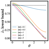
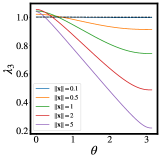
In contrast with LReLU activations, such a degeneracy guarantee does not exist for GELU and ELU activations. For both the GELU and ELU, we consider the dynamics on a ball of constant $\|\mathbf{x}\|$, where $\sigma_{w}$ is chosen such that $g_{1}=\|\mathbf{x}\|$. In Figure 4, for different values of $\|\mathbf{x}\|$ in the context of Corollary 8, we evaluate a lower bound for $\lambda_{3}$ in the case of GELU and $\lambda_{3}$ exactly in the case of ELU. Full working is given in Appendices G.1 and G.2. We observe that each exceeds $1$ at some point on the (but not over the whole) interval, and is therefore not a contraction mapping and hence not guaranteed to have a unique fixed point. This is consistent with Figures 2 and 3, where fixed points are shown by intersecting curves.

5 Extension of theoretical results to NTK

We may also study kernel fixed points of infinitely wide neural networks trained under gradient flow. This amounts to studying the fixed point properties of the neural tangent kernel (NTK). If such a unique fixed point exists, this implies that the functions obtained by applying gradient flow to an infinitely wide, infinitely deep MLP are also degenerate. In this section, we briefly sketch how such a result may be obtained. We leave the presentation of formal results and empirical evaluations for future work.

Informally, the value of the eigenvalue $\lambda_{3}$ can still predict the fixed point behaviour of the NTK. Formally, the result is slightly more involved, see Appendix I. Consider a state space $\mathcal{S}\subset\mathbb{R}^{4}$ containing states $(s_{1}^{2},s_{2}^{2},k,T)$ consisting of squared norms for both inputs, the kernel, and the NTK. We update the states through $\mathbf{h}:\mathcal{S}\to\mathcal{S}$:

$$h_{i}(s_{1}^{2},s_{2}^{2},k,T) =\sigma_{w}^{2}\mathbb{E}\big{[}\psi^{2}(s_{i}Z_{i})\big{]}+\sigma_{b}^{2},\quad i=i,2$$

$$h_{3}(s_{1}^{2},s_{2}^{2},k,T) =\sigma_{w}^{2}\mathbb{E}\big{[}\psi(s_{1}Z_{1})\psi(s_{2}Z_{2})\big{]}+\sigma_{b}^{2},$$

$$h_{4}(s_{1}^{2},s_{2}^{2},k,T) =T\sigma_{w}^{2}\mathbb{E}\big{[}\psi^{\prime}(s_{1}Z_{1})\psi^{\prime}(s_{2}Z_{2})\big{]}+$$

$$\phantom{{}={}}\sigma_{w}^{2}\mathbb{E}\big{[}\psi(s_{1}Z_{1})\psi(s_{2}Z_{2})\big{]}+\sigma_{b}^{2},$$

where $\text{Cov}(Z_{1},Z_{2})=k/(s_{1}s_{2})$, $\mathbb{E}[Z_{1}]=\mathbb{E}[Z_{2}]=0$. As in Corollary 8, if a fixed point of the system only involving $s_{1}$ and $h_{1}$ exists at a value $\sigma_{w}=\sigma^{*}$ and $s_{1}=s_{2}=s$, then the system reduces to a $2$ dimensional update involving only $h_{3}$ and $h_{4}$ along $s_{1}=s_{2}=s$. The Jacobian is diagonal,

$$J=\begin{pmatrix}\frac{\partial h_{3}}{\partial k}&\frac{\partial h_{3}}{\partial T}\\ \frac{\partial h_{4}}{\partial k}&\frac{\partial h_{4}}{\partial T}\end{pmatrix} =\begin{pmatrix}\frac{\partial h_{3}}{\partial k}&0\\ \frac{\partial h_{4}}{\partial k}&\frac{\partial h_{4}}{\partial T}\end{pmatrix},$$

so the eigenvalues are $\frac{\partial h_{3}}{\partial k}$ and $\frac{\partial h_{4}}{\partial T}$. By Theorem 6,

$$\frac{\partial h_{3}}{\partial k}=\frac{\partial h_{3}}{\partial\rho}\Big{(}\frac{\partial k}{\partial\rho}\Big{)}^{-1}=\frac{\partial g_{3}}{\partial\rho}\sqrt{h_{1}h_{2}}(s_{1}s_{2})^{-1}$$

$$=(\sigma^{*})^{2}\mathbb{E}\big{[}\psi^{\prime}(s_{1}Z_{1})\psi^{\prime}(s_{2}Z_{2})\big{]}=\frac{\partial h_{4}}{\partial T}=\lambda_{3}.$$

6 Gaussian process experiments

We perform two sets of experiments. In the first, we investigate the performance of GPs with various neural network kernels. In the second, we observe the degree of implicit regularisation that is obtained using GPs of finite depth.

6.1 Benchmarking

We provide a software implementation of our new kernels. To demonstrate usage of our covariance functions, first we compare the performance of GP regression models using ReLU, LReLU, ERF and GELU kernels on a popular Bayesian deep learning benchmark (Hernández-Lobato and Adams 2015). The purpose of these experiments is not to showcase the superiority of one prior over another, but rather to provide a sample implementation. This implementation has already been ported over to another framework in concurrent work by others (Novak et al. 2020). The ELU kernel was not included in our experiments (see § 3). We perform separate experiments on shallow models having $1$ hidden layer and deep models having up to $32$ hidden layers. All data was standardised to have mean $0$ and variance $1$.

Figure 5: RMSE for equivalent single-hidden-layer GPs. Mean $\pm 2$ standard errors (over 20 runs).

Figure 6: Posterior predictive $\pm 2$ standard deviations.

Figure 7: RMSE against $\sigma_{w}^{2}$ for equivalent $l$ layer GPs, Wine dataset. Shaded region shows $\pm 1$ standard deviation. (Clockwise from top left) ReLU, GELU, LReLU, ERF.

Table 1: Best performing models for each kernel over the grid search.

		ReLU			GELU			LReLU			ERF
	RMSE	$\sigma_{w}^{2}$	$\ell$	RMSE	$\sigma_{w}^{2}$	$\ell$	RMSE	$\sigma_{w}^{2}$	$\ell$	RMSE	$\sigma_{w}^{2}$	$\ell$
Boston	$2.85\pm 0.64$	$1.90$	$7$	$2.86\pm 0.65$	$1.80$	$6$	$\mathbf{2.60\pm 1.07}$	$\mathbf{2.00}$	$\mathbf{32}$	$2.69\pm 0.95$	$5.00$	$2$
Concrete	$5.22\pm 0.55$	$5.00$	$2$	$\mathbf{5.21\pm 0.56}$	$\mathbf{5.00}$	$\mathbf{2}$	$5.23\pm 0.44$	$3.30$	$3$	$5.63\pm 0.46$	$5.00$	$2$
Energy	$\mathbf{0.89\pm 0.11}$	$\mathbf{5.00}$	$\mathbf{2}$	$0.92\pm 0.12$	$5.00$	$2$	$2.77\pm 0.31$	$0.10$	$1$	$2.79\pm 0.23$	$0.10$	$1$
Wine	$1.15\pm 0.13$	$5.00$	$4$	$1.17\pm 0.14$	$5.00$	$4$	$\mathbf{1.04\pm 0.12}$	$\mathbf{5.00}$	$\mathbf{5}$	$3.96\pm 0.75$	$5.00$	$1$
Yacht	$0.58\pm 0.01$	$4.80$	$32$	$0.58\pm 0.01$	$2.30$	$32$	$0.60\pm 0.02$	$1.80$	$29$	$\mathbf{0.57\pm 0.02}$	$\mathbf{5.00}$	$\mathbf{8}$

Shallow models.

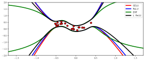
Do differences in priors induced by the various activation functions affect empirical performance? Using the limiting GP allows us to remove the interaction between $\psi$ and optimisation, and purely consider the effect of $\psi$ on the functional prior. Figure 6 shows the predictive distribution of GPs with GELU, ReLU, LReLU and ERF kernels on a toy regression task. ERF has different extrapolation properties due to being a bounded activation, whilst the others appear qualitatively similar, though with extrapolation variance decreasing in the order GELU/ReLU/LReLU.

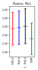
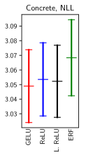
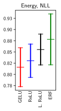
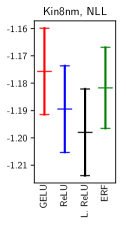
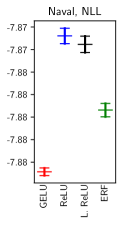
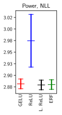
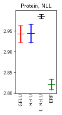
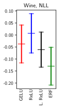
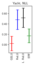
Figure 5 shows benchmark results for single-hidden-layer GPs using a 90%/10% training/test split. See Appendix J.1 for more details and plots. All kernels perform comparably; gains can be made by selecting a kernel suited to the dataset. Results are most different for ERF — either negatively (Concrete, Energy) or positively (Boston, Protein, Wine). Differences are observed between GELU/ReLU/LReLU. For example, GELU offers an advantage in Naval and Yacht, and LReLU performs poorly on Protein.

None of the kernels consistently outperform the others. This is expected behaviour, similar to how a Matern kernel might outperform a squared exponential kernel only some of the time on real-world datasets. The purpose of the experiment was to evaluate whether different $\psi$ result in a strong enough difference in priors that empirical performance differences can be observed. Having answered in the positive, we posit that for finite-width networks, the difference in performance found by varying $\psi$ may partially derive from differences in the induced prior. This is in contrast to previously cited reasons such as bias shift and its relation to natural gradient (Clevert, Unterthiner, and Hochreiter 2016).

Deep models.

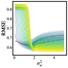
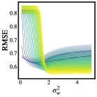
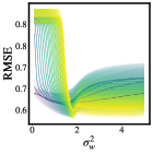
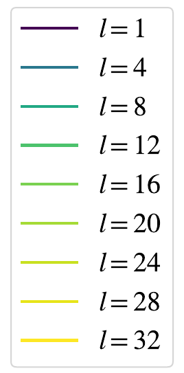
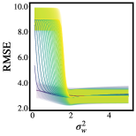
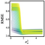
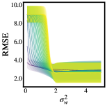
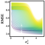
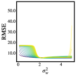
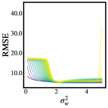
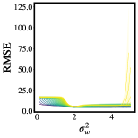
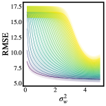
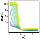
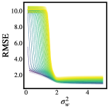
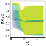
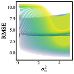
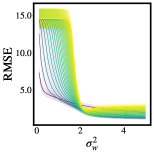
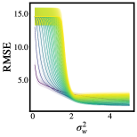
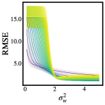
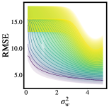
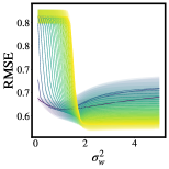
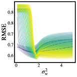
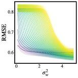
How does the performance of models vary with depth? We randomly shuffled the data into an $80/20\%$ train/test split $5$ times. For each split, we ran GP regression with an additive iid Gaussian noise model having variance fixed at $0.1$. We varied the depth $\ell\in[1,32]$ in steps of $1$ and the weight and bias variances (which were constrained to be equal in each layer) $\sigma_{w}^{2}\in[0.1,5]$ in steps of $0.1$. For each setting, we measured the RMSE between the mean of the GP prediction and the true regression targets. Figure 7 shows the average RMSE on the Wine dataset over $5$ shuffles. Other datasets are given in Appendix J.2. We make two qualitative observations. Firstly, $\ell>1$ models out-perform $\ell=1$ models. Secondly, the RMSE changes smoothly in both depth and $\sigma_{w}^{2}$. The visual smoothness is not due to averaging over $5$ trials; smoothness is also observed when we plot results from only $1$ random shuffling. Table 1 shows the best models obtained over the grid search for each kernel.

6.2 Overfitting and underfitting

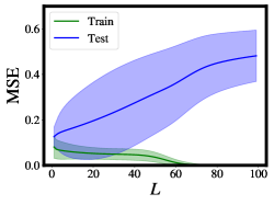
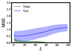
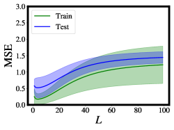
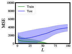
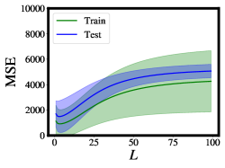
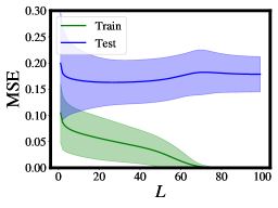
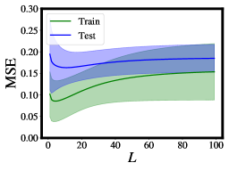
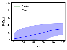
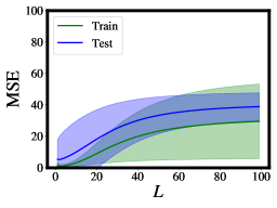
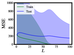
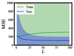
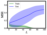
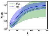
We empirically investigate the relationship between depth and training/testing error. When the covariance function has a unique fixed point, we expect to see underfitting at large depth, since large depth will push the kernel towards the unique fixed point, that is, a constant normalised kernel. On the other hand, when the covariance function does not have a unique fixed point, we might expect to see overfitting as model complexity may increase with depth.

We build predictor variables of a training dataset by uniformly sampling $\mathbf{x}\in\mathbb{R}^{2}$ on the unit disc at heading $\gamma$. We then sample training targets through the mapping $y=f(\gamma)+\epsilon$ for a number of different choices of $f$, where $\epsilon$ is additive Gaussian noise with variance fixed at $0.1$. We find the posterior predictive mean of a Gaussian process with iterated GELU and ReLU covariance functions of depth $L$ between $1$ and $100$ with a choice of $\sigma_{w}$ according to Figure 4. We repeat this process with a new random training set $10$ times. Each repetition, we find the mean-squared error (MSE) between the posterior mean of the Gaussian process over the training set and a test set built from a (deterministic) uniform grid of size $100$. Figure 8 shows the resulting train and test errors on one choice of $f$, and Appendix L shows other choices of $f$. Figure 1 shows a more direct illustration of the function fit on one of the random data samples, with other choices of $f$ shown in Appendix L.

Figure 8: Training and testing errors for GPs with covariance functions corresponding to infinitely wide MLPs of increasing depth $L$ using the same example as in Figure 1. Solid curve shows the mean over $10$ training data samples, and the shaded region shows $\pm$ two standard deviations. By examining whether the training and testing error increases or decreases with depth, we observe that the GELU and ReLU respectively overfit and underfit with depth. See Appendix L for more error curves. (Left) GELU (Right) ReLU.

7 Discussion and conclusion

We introduced two new positive semi-definite kernels arising from the infinite-width limit of Bayesian GELU or ELU NNs. We provided visualisations of these kernels for varying depths. We introduced a general framework for understanding the fixed-point dynamics of such kernels and their NTK counterparts. Using this framework, we showed that unlike the ReLU, the GELU and ELU kernels are able to avoid unique fixed points. We empirically verified that finite-width NNs are able to avoid unique kernel fixed points in Figures 2 and 3. We applied our kernels in the setting of shallow and deep GP regression, finding that for some problems specific kernels are more appropriate, and that the GELU kernel is competitive with the ReLU kernel.

Investigations into implicit regularisation consider the role of one or all of (a) the architecture, (b) the learning algorithm and (c) the data sampling process. Neyshabur, Tomioka, and Srebro (2015) argue that (b) leads implicitly to low-norm solutions, explaining the generalisation ability of deep NNs. On the other hand, Dereziński, Liang, and Mahoney (2019) construct a data sampling distribution (c) that explains double descent and implicit regularisation in linear models. Similar to our work but not considering the NTK, the signal propagation literature (Schoenholz et al. 2017; Poole et al. 2016) explains simplicity biases in randomly initialised networks (a). They develop objects similar to $\frac{\partial g_{3}}{\partial\rho}$, but require bounded activations, and seem to also require some notion of differentiability. Our analysis considers (a) and (b) but not (c). We have recently been made aware of the concurrent work of (Huang et al. 2020), who also study the degeneracy of processes induced through ReLU activations. Their focus is on both (a) and (b), arguing that the NTK for residual architectures does not suffer from this degeneracy.

Knowing the gradient of the kernel with respect to $(\sigma_{w}^{(l)})^{2}$ and $(\sigma_{b}^{(l)})^{2}$ is useful for both empirical Bayesian methodologies (e.g. optimising the marginal likelihood using LBFGS) and hierarchical models (e.g. using HMC to integrate out the hyperprior). As we detail in Appendix K, our results may be used to find this gradient. Theorem 6 provides $7$ of the $9$ elements of the Jacobian. The other $2$ can only easily be evaluated in special cases (e.g. LReLU results in a diagonal Jacobian). In future work, it may be interesting to extend Theorem 6 to cover the remaining elements of the Jacobian.

While Lee et al. (2019) found close agreement between NNs and their corresponding limiting GPs, several authors (Neal 1995; MacKay 2003; Der and Lee 2006; Matthews et al. 2018; Chizat, Oyallon, and Bach 2019; Tsuchida, Roosta, and Gallagher 2019b; Allen-Zhu, Li, and Liang 2019; Favaro, Fortini, and Peluchetti 2020; Aitchison 2020) have argued against the use of GP models as a means to understand the success of deep learning. If deep learning’s performance can be explained using GPs, why do NN models outperform their limiting GP counterparts? Arora et al. (2019) attain $77\%$ test accuracy on CIFAR10 using a limiting GP arising from a trained CNN, while a ResNet is able to achieve $96\%$ (Springenberg et al. 2015). On the other hand, Arora et al. (2020) find that GP models are competitive on small datasets. It remains to determine if this difference in performance is due to the tricks for which equivalence in the GP setting have not yet been fully explored, or if it is the result of some deeper property of GPs. Lee et al. (2020) empirically explore some of these questions including the effects of finite width, architectures, weight decay and the performance difference between infinite Bayesian and NTK models. While we acknowledge the limitations of the infinitely wide approach, we believe it warrants further exploration, if not to understand the power of deep learning, at least to investigate its generalisation abilities. The purpose of our study was not to optimise any architecture for performance on a particular problem, but rather to develop results under the GP framework that contribute to our understanding of generalisation in the overparameterised setting.

Appendix A Derivation of GELU kernel

We would like to evaluate the kernel (up to a scaling and offset)

$$k(\mathbf{x}_{1},\mathbf{x}_{2})=s_{1}s_{2}\mathbb{E}\Big{[} Z_{1}Z_{2}\Phi(s_{1}Z_{1})\Phi\big{(}s_{2}Z_{2}\big{)}\Big{]}.$$

We split our evaluation of the kernel into two cases, first when $\theta\in(0,\pi)$, and second when $\theta\in\{0,\pi\}$.

A.1 $\theta\in(0,\pi)$

We introduce dummy variables $\beta_{1},\beta_{2}$ and define

$$\kappa(\beta_{1},\beta_{2})=s_{1}s_{2}\mathbb{E}\Big{[}Z_{1}Z_{2}\Phi\Big{(}\beta_{1}s_{1}Z_{1}\Big{)}\Phi\Big{(}\beta_{2}s_{2}Z_{2}\Big{)}\Big{]}.$$

The mixed derivative $\frac{\partial^{2}\kappa}{\partial\beta_{1}\,\partial\beta_{2}}$ is

$$s_{1}^{2}s_{2}^{2}\mathbb{E}\Big{[}Z_{1}^{2}Z_{2}^{2}\phi\Big{(}\beta_{1}s_{1}Z_{1}\Big{)}\phi\Big{(}\beta_{2}s_{2}Z_{2}\Big{)}\Big{]}$$

$$=s_{1}^{2}s_{2}^{2}\int z_{1}^{2}z_{2}^{2}\phi\Big{(}\beta_{1}s_{1}z_{1}\Big{)}\phi\Big{(}\beta_{2}s_{2}z_{2}\Big{)}\phi_{2}(z_{1},z_{2})\,dz_{1}\,dz_{2}.$$ (5)

The product of the normal PDFs is given by

$$\frac{1}{2\pi\sin\theta}\Big{(}\frac{1}{\sqrt{2\pi}}\Big{)}^{2}\exp\Big{(}-\frac{1}{2}(\mathbf{z}^{\top}S^{-1}\mathbf{z}+\mathbf{z}^{\top}\beta\mathbf{z})\Big{)},$$

where $S^{-1}=\frac{1}{\sin^{2}\theta}\begin{bmatrix}1&-\cos\theta\\ -\cos\theta&1\end{bmatrix}$ and $\beta=\begin{bmatrix}s_{1}^{2}\beta_{1}^{2}&0\\ 0&s_{2}^{2}\beta_{2}^{2}\end{bmatrix}$. Now $S^{-1}+\beta$ is the inverse of a positive definite covariance matrix, with

$$S^{-1}+\beta =\frac{1}{\sin^{2}\theta}\begin{bmatrix}1+s_{1}^{2}\beta_{1}^{2}\sin^{2}\theta&-\cos\theta\\ -\cos\theta&1+s_{2}^{2}\beta_{2}^{2}\sin^{2}\theta\end{bmatrix},$$

having determinant

$$\csc^{4}\theta\big{(}(1+s_{1}^{2}\beta_{1}^{2}\sin^{2}\theta)(1+s_{2}^{2}\beta_{2}^{2}\sin^{2}\theta)-\cos^{2}\theta\big{)}$$

and inverse

$$\big{(}(1+s_{1}^{2}\beta_{1}^{2}\sin^{2}\theta)(1+s_{2}^{2}\beta_{2}^{2}\sin^{2}\theta)-\cos^{2}\theta\big{)}^{-1}$$

$$\phantom{{}={}}\sin^{2}\theta\begin{bmatrix}1+s_{2}^{2}\beta_{2}^{2}\sin^{2}\theta&\cos\theta\\ \cos\theta&1+s_{1}^{1}\beta_{2}^{2}\sin^{2}\theta\end{bmatrix}.$$

We may therefore write (5) as

$$\frac{s_{1}^{2}s_{2}^{2}}{2\pi\sin\theta}\det(S^{-1}+\beta)^{-\frac{1}{2}}\mathbb{E}[U_{1}^{2}U_{2}^{2}],$$

where $(U_{1},U_{2})^{\top}$ has covariance matrix $C=(S^{-1}+\beta)^{-1}$. The expectation $\mathbb{E}[U_{1}^{2}U_{2}^{2}]$ has a known form, and is given by

$$\mathbb{E}[U_{1}^{2}U_{2}^{2}] =C_{11}C_{22}+2C_{12}^{2}$$

$$=\big{(}(1+s_{1}^{2}\beta_{1}^{2}\sin^{2}\theta)(1+s_{2}^{2}\beta_{2}^{2}\sin^{2}\theta)-\cos^{2}\theta\big{)}^{-2}$$

$$\phantom{{}={}}\big{(}(1+s_{1}^{2}\beta_{1}^{2}\sin^{2}\theta)(1+s_{2}^{2}\beta_{2}^{2}\sin^{2}\theta)+2\cos^{2}\theta\big{)}$$

$$\phantom{{}={}}\sin^{4}\theta.$$

Finally,

$$\frac{\partial^{2}\kappa}{\partial\beta_{1}\,\partial\beta_{2}} =\frac{\sin^{5}\theta s_{1}^{2}s_{2}^{2}}{2\pi}$$

$$\Big{[}\big{(}(1+s_{1}^{2}\beta_{1}^{2}\sin^{2}\theta)(1+s_{2}^{2}\beta_{2}^{2}\sin^{2}\theta)-\cos^{2}\theta\big{)}^{-5/2}$$

$$\big{(}(1+s_{1}^{2}\beta_{1}^{2}\sin^{2}\theta)(1+s_{2}^{2}\beta_{2}^{2}\sin^{2}\theta)+2\cos^{2}\theta\big{)}\Big{]}.$$

We also have the boundary conditions

$$\frac{\partial\kappa}{\partial\beta_{1}}\Big{|}_{\beta_{2}=0}=\frac{\partial\kappa}{\partial\beta_{2}}\Big{|}_{\beta_{1}=0} =0,\quad\text{ and}$$

$$\kappa(0,0) =\frac{s_{1}s_{2}}{4}\cos\theta.$$

The solution to this PDE can be found by direct integration with integration constants due to the conditions. The solution evaluated at $\beta_{1}=\beta_{2}=1$ is

$$\frac{s_{1}^{2}s_{2}^{2}}{2\pi}\Big{[}\frac{\frac{1}{2}(\cos(2\theta)+3)+s_{1}^{2}+s_{2}^{2}+s_{1}^{2}s_{2}^{2}\sin^{2}\theta}{(1+s_{1}^{2})(1+s_{2}^{2})\sqrt{1+s_{1}^{2}+s_{2}^{2}+s_{1}^{2}s_{2}^{2}\sin^{2}\theta}}$$

$$+ \frac{\cos\theta}{s_{1}s_{2}}\tan^{-1}\Big{(}\frac{\cos\theta s_{1}s_{2}}{\sqrt{1+s_{1}^{2}+s_{2}^{2}+s_{1}^{2}s_{2}^{2}\sin^{2}\theta}}\Big{)}\Big{]}+\frac{s_{1}s_{2}}{4}\cos\theta.$$

A.2 $\theta\in\{0,\pi\}$

We may simply evaluate the result obtained on $(0,\pi)$ at $0$ and $\pi$. To see this, observe that $k$ is continuous with respect to $\theta$ on $[0,\pi]$. Firstly,

$$\psi(s_{1}Z_{1})\psi\big{(}s_{2}Z_{2}) \leq\max\{\psi^{2}(s_{1}Z_{1}),\psi^{2}(s_{2}Z_{2})\}$$

$$\leq\psi^{2}(s_{1}Z_{1})+\psi^{2}(s_{2}Z_{2}),$$

which has finite expectation. Let $G_{1}\mathchoice{\mathrel{\hbox to0.0pt{$\displaystyle\perp$\hss}\mkern 2.0mu{\displaystyle\perp}}}{\mathrel{\hbox to0.0pt{$\textstyle\perp$\hss}\mkern 2.0mu{\textstyle\perp}}}{\mathrel{\hbox to0.0pt{$\scriptstyle\perp$\hss}\mkern 2.0mu{\scriptstyle\perp}}}{\mathrel{\hbox to0.0pt{$\scriptscriptstyle\perp$\hss}\mkern 2.0mu{\scriptscriptstyle\perp}}}G_{2}\sim\mathcal{N}(0,1)$. By dominated convergence,

$$\phantom{{}={}}\lim_{\theta\to 0}k(\cos\theta)$$

$$=\mathbb{E}\big{[}\lim_{\theta\to 0}\psi\big{(}s_{1}G_{1}\big{)}\psi\big{(}s_{2}(\cos\theta G_{1}+\sqrt{1-\cos^{2}\theta}G_{2})\big{)}\big{]}$$

$$=\mathbb{E}\big{[}\psi\big{(}s_{1}G_{1}\big{)}\psi\big{(}s_{2}G_{1}\big{)}\big{]}$$

$$=k(1),$$

and similarly for the case $\theta\to\pi$.

Appendix B Derivation of ELU kernel

We would like to evaluate the kernel (up to a scaling and offset)

$$\mathbb{E}\Big{[} \Big{(}\lambda\Theta(\widetilde{Z}_{1}{+}\widetilde{\mu}_{1})\big{(}\widetilde{Z}_{1}{+}\widetilde{\mu}_{1}\big{)}+\lambda\alpha\Theta(-\widetilde{Z}_{1}{-}\widetilde{\mu}_{1})\big{(}e^{\widetilde{Z}_{1}+\widetilde{\mu}_{1}}{-}1\big{)}\Big{)}$$

$$\Big{(}\lambda\Theta(\widetilde{Z}_{2}{+}\widetilde{\mu}_{2})\big{(}\widetilde{Z}_{2}{+}\widetilde{\mu}_{2}\big{)}+\lambda\alpha\Theta(-\widetilde{Z}_{2}{-}\widetilde{\mu}_{2})\big{(}e^{\widetilde{Z}_{2}+\widetilde{\mu}_{2}}{-}1\big{)}\Big{)}\Big{]},$$

where $\widetilde{Z}_{i}=s_{i}Z_{i}$. Note we have included parameters $\lambda$ and $\alpha$ corresponding to the SELU, which recovers the ELU when $\lambda=\alpha=1$. We may expand the expectation into the sum of

$$E_{1} =\lambda^{2}\mathbb{E}\Big{[}\Theta(\widetilde{Z}_{1}{+}\widetilde{\mu}_{1})(\widetilde{Z}_{1}{+}\widetilde{\mu}_{1})\Theta(\widetilde{Z}_{2}{+}\widetilde{\mu}_{2})(\widetilde{Z}_{2}{-}\widetilde{\mu}_{2})\Big{]},$$ (6)

$$E_{2} =\lambda^{2}\alpha\mathbb{E}\Big{[}\Theta(\widetilde{Z}_{1}{+}\widetilde{\mu}_{1})(\widetilde{Z}_{1}+\widetilde{\mu}_{1})\Theta(-\widetilde{Z}_{2}{-}\widetilde{\mu}_{2})\big{(}e^{\widetilde{Z}_{2}{+}\widetilde{\mu}_{2}}{-}1\big{)}\Big{]},$$ (7)

$$E_{3} =\lambda^{2}\alpha\mathbb{E}\Big{[}\Theta(\widetilde{Z}_{2}{+}\widetilde{\mu}_{2})(\widetilde{Z}_{2}{+}\widetilde{\mu}_{2})\Theta(-\widetilde{Z}_{1}{-}\widetilde{\mu}_{1})\big{(}e^{\widetilde{Z}_{1}+\widetilde{\mu}_{1}}{-}1\big{)}\Big{]},$$ (8)

and

$$E_{4}=\lambda^{2}\alpha^{2}\mathbb{E}\Big{[} \Theta(-\widetilde{Z}_{1}{-}\widetilde{\mu}_{1})\big{(}e^{\widetilde{Z}_{1}+\widetilde{\mu}_{1}}{-}1\big{)}\Theta(-\widetilde{Z}_{2}{-}\widetilde{\mu}_{2})\big{(}e^{\widetilde{Z}_{2}+\widetilde{\mu}_{2}}{-}1\big{)}\Big{]}.$$ (9)

In the following sections we evaluate each term in the sum. It suffices to evaluate the kernel on the open interval $(0,\pi)$ by the same argument as in § A.2.

B.1 $E_{1}$

The integral (6) is a non-trivial generalisation of the arc-cosine kernel of degree $1$ (Cho and Saul 2009) with $\bm{\mu}\neq 0$, and is evaluated by Tsuchida, Roosta, and Gallagher (2019b).

B.2 $E_{2}$ and $E_{3}$

The second integral in (7) is

$$\frac{s_{1}}{2\pi\sin\theta}\int_{\mathbb{R}^{2}} \Theta(z_{1}+\widetilde{\mu}_{1}/s_{1})(z_{1}+\widetilde{\mu}_{1}/s_{1})\Theta(-z_{2}-\widetilde{\mu}_{2}/s_{2})$$

$$\big{(}e^{s_{2}z_{2}-\widetilde{\mu}_{2}}-1\big{)}\exp\Big{(}-\frac{1}{2}\mathbf{z}^{\top}S^{-1}\mathbf{z}\Big{)}\,dz_{1}\,dz_{2}.$$

We may complete the square of the exponentiated terms,

$$\phantom{{}={}}\exp\Big{(}-\frac{1}{2}\big{(}\mathbf{z}^{\top}S^{-1}\mathbf{z}-2s_{2}z_{2}\big{)}\Big{)}$$

$$=\exp\Big{(}-\frac{1}{2}\Big{(}\big{(}\mathbf{z}-s_{2}S_{:,2}\big{)}^{\top}S^{-1}\big{(}\mathbf{z}-s_{2}S_{:,2}\big{)}-s_{2}^{2}\Big{)}\Big{)},$$

where $S_{:,2}$ denotes the second column of $S$. $E_{2}$ is then

$$\phantom{{}={}}e^{-\widetilde{\mu}_{2}+s_{2}^{2}/2}s_{1}\mathbb{E}\Big{[}\Theta(Z_{1}+s_{2}\cos\theta+\widetilde{\mu}_{1}/s_{1})$$

$$\phantom{{}={}}(Z_{1}+s_{2}\cos\theta+\widetilde{\mu}_{1}/s_{1})\Theta(-Z_{2}-s_{2}-\widetilde{\mu}_{2}/s_{2})\Big{]}-$$

$$\phantom{{}={}}s_{1}\mathbb{E}\Big{[}\Theta(Z_{1}+\widetilde{\mu}_{1}/s_{1})(Z_{1}+\widetilde{\mu}_{1}/s_{1})\Theta(-Z_{2}-\widetilde{\mu}_{2}/s_{2})\Big{]}.$$

Both of these expectations can be related to the first moment of the truncated standard bivariate normal distribution, which has a known form. Let $(Y_{1},Y_{2})$ be distributed according to the standard bivariate normal distribution with correlation $-\cos\theta$, and let $h,k\in\mathbb{R}$. Defining $M$ for convenience as follows, Rosenbaum (1961) gives

$$\phantom{{}={}}M(h,k)$$

$$=\mathbb{E}\Big{[}\Theta(Y_{1}-h)Y_{1}\Theta(Y_{2}-k)\Big{]}$$

$$=\frac{1}{2\pi\sin\theta}\int_{k}^{\infty}\int_{h}^{\infty}z_{1}\exp\Big{(}-\frac{1}{2\sin^{2}\theta}(z_{1}^{2}+2\cos\theta z_{1}z_{2}+z_{2}^{2})\Big{)}\,dz_{1}\,dz_{2}$$

$$=\phi(h)\Bigg{(}1-\bm{\Phi}\Big{(}\frac{k+h\cos\theta}{\sin\theta}\Big{)}\Bigg{)}-\cos\theta\phi(k)\Bigg{(}1-\bm{\Phi}\Big{(}\frac{h+k\cos\theta}{\sin\theta}\Big{)}\Bigg{)}.$$

Therefore,

$$\phantom{{}={}}s_{1}\mathbb{E}\Big{[}\Theta(Z_{1}+\widetilde{\mu}_{1}/s_{1})(Z_{1}+\widetilde{\mu}_{1}/s_{1})\Theta(-Z_{2}-\widetilde{\mu}_{2}/s_{2})\Big{]}$$

$$=s_{1}\Bigg{(}M\Big{(}-\frac{\widetilde{\mu}_{1}}{s_{1}},\frac{\widetilde{\mu}_{2}}{s_{2}}\Big{)}+\frac{\widetilde{\mu}_{1}}{s_{1}}\Phi\Big{(}-\frac{\widetilde{\mu}_{1}}{s_{1}},\frac{\widetilde{\mu}_{2}}{s_{2}};-\cos\theta\Big{)}\Bigg{)},$$

and

$$\phantom{{}={}}\mathbb{E}\Big{[}\Theta(Z_{1}+s_{2}\cos\theta+\widetilde{\mu}_{1}/s_{1})(Z_{1}+s_{2}\cos\theta+\widetilde{\mu}_{1}/s_{1})\Theta(-Z_{2}-s_{2}-\widetilde{\mu}_{2}/s_{2})\Big{]}$$

$$=M\Big{(}-s_{2}\cos\theta-\frac{\widetilde{\mu}_{1}}{s_{1}},s_{2}+\frac{\widetilde{\mu}_{2}}{s_{2}}\Big{)}+\Big{(}s_{2}\cos+\frac{\widetilde{\mu}_{1}}{s_{1}}\Big{)}\Phi\Big{(}s_{2}\cos\theta-\frac{\widetilde{\mu}_{1}}{s_{1}},-s_{2}+\frac{\widetilde{\mu}_{2}}{s_{2}};-\cos\theta\Big{)}.$$

B.3 $E_{4}$

$$E_{4} =\lambda^{2}\alpha^{2}\mathbb{E}\Big{[}\Theta(-Z_{1}-\widetilde{\mu}_{1}/s_{1})\Theta(-Z_{2}-\widetilde{\mu}_{2}/s_{2})\big{(}e^{s_{1}Z_{1}+s_{2}Z_{2}+\widetilde{\mu}_{1}+\widetilde{\mu}_{2}}-e^{s_{1}Z_{1}+\widetilde{\mu}_{1}}-e^{s_{2}Z_{2}+\widetilde{\mu}_{2}}+1\big{)}\Big{]}.$$

Each of the four terms may be understood as scales of special cases of the function

$$e_{4}(a,b) =\mathbb{E}\Big{[}\Theta(-Z_{1}-\widetilde{\mu}_{1}/s_{1})\Theta(-Z_{2}-\widetilde{\mu}_{2}/s_{2})e^{aZ_{1}+bZ_{2}}\Big{]}$$

for $a,b\in\mathbb{R}$. Completing the square, $e_{4}(a,b)$ is given by

$$\phantom{{}={}}\int_{-\infty}^{-\widetilde{\mu}_{2}/s_{2}}\int_{-\infty}^{-\widetilde{\mu}_{1}/s_{1}}\frac{1}{2\pi\sin\theta}\exp\Big{(}-\frac{1}{2}(\mathbf{z}^{\top}\Sigma^{-1}\mathbf{z}-2az_{1}-2bz_{2})\Big{)}\,dz_{1}\,dz_{2}$$

$$=\int_{\widetilde{\mu}_{2}/s_{2}}^{\infty}\int_{\widetilde{\mu}_{1}/s_{1}}^{\infty}\frac{1}{2\pi\sin\theta}\exp\Big{(}-\frac{1}{2}(\mathbf{z}^{\top}\Sigma^{-1}\mathbf{z}+2az_{1}+2bz_{2})\Big{)}\,dz_{1}\,dz_{2}$$

$$=\frac{\exp\Big{(}\frac{1}{2}(a,b)\Sigma(a,b)^{\top}\Big{)}}{2\pi\sin\theta}\int_{\widetilde{\mu}_{2}/s_{2}}^{\infty}\int_{\widetilde{\mu}_{1}/s_{1}}^{\infty}\,dz_{1}\,dz_{2}\exp\Big{(}-\frac{1}{2}\big{(}\mathbf{z}+\Sigma(a,b)^{\top}\big{)}^{\top}\Sigma^{-1}\big{(}\mathbf{z}+\Sigma(a,b)^{\top}\big{)}\Big{)}$$

$$=\Phi\big{(}(\widetilde{\mu}_{1}/s_{1},\widetilde{\mu}_{2}/s_{2})^{\top}-\Sigma(a,b)^{\top};\cos\theta\big{)}\exp\Big{(}\frac{1}{2}(a,b)\Sigma(a,b)^{\top}\Big{)}.$$

Appendix C Proof of Theorem 6

We are interested in studying expectations of objects that may not be integrable functions with respect to the Gaussian measure, namely tempered distributions. In order to do so, we denote the set of Schwartz functions on the plane by $D(\mathbb{R}^{2})$ and its dual space, the space of tempered distributions, by $D^{\prime}(\mathbb{R}^{2})$, and observe that $\phi\in D(\mathbb{R}^{2})$. For $q\in D(\mathbb{R}^{2})$ and $T\in D^{\prime}(\mathbb{R}^{2})$, write $\langle T\,,\,q\rangle$ for the dual pairing of $T$ and $q$. For any $q\in D(\mathbb{R}^{2})$ we can then define an operator $q^{\star}$ on $D^{\prime}(\mathbb{R}^{2})$ via the natural injection into the dual space of $D^{\prime}(\mathbb{R}^{2})$ by setting $q^{\star}(T)=\langle T,q\rangle$ for any $T\in D^{\prime}(\mathbb{R}^{2})$. We can then define the expectation of the distribution by defining $\mathbb{E}[T]=\langle T,\phi\rangle$, which agrees with the usual definition whenever $T$ can be represented by an integrable function. Following Jones (1982), we define the derivative of a tempered distribution via $\langle\frac{\partial}{\partial x}T\,,\,q\rangle=-\langle T\,,\,\frac{\partial}{\partial x}q\rangle$, and when $T$ can be represented by a locally integrable function $f$, we abuse notation to write $\int_{\mathbb{R}^{2}}\frac{\partial f}{\partial x}\phi:=-\int_{\mathbb{R}^{2}}f\frac{\partial\phi}{\partial x}.$ This is analogously extended for higher order derivatives by ensuring integration by parts holds whenever $f$ is smooth.

Proof.

We begin by evaluating the derivative of $g_{3}$ with respect to $\rho$. Let $\bm{\omega}$ denote the Lebesgue measure. Note that the mapping $T_{\psi}:D(\mathbb{R}^{2})\to\mathbb{R}$ satisfying

$$T_{\psi}(q)=\int\psi(s_{1}\omega_{1})\psi\big{(}s_{2}(\omega_{1}\rho+\omega_{2}\sqrt{1-\rho^{2}})\big{)}q(\bm{\omega})d\bm{\omega}$$

is a tempered distribution since for all $q\in D(\mathbb{R}^{2})$,

$$\phantom{{}\leq{}}\int\Big{|}\psi(s_{1}\omega_{1})\psi\big{(}s_{2}(\omega_{1}\rho+\omega_{2}\sqrt{1-\rho^{2}})q(\bm{\omega})\big{)}\Big{|}d\bm{\omega}\leq\int p(\bm{\omega})\Big{|}q(\bm{\omega})\Big{|}d\bm{\omega}<\infty,$$

where $p$ is some polynomial. Let $\phi_{\rho}$ denote the PDF of a standard bivariate Gaussian with correlation $\rho$. Differentiating $g_{3}$ with respect to $\rho$ we find

$$\frac{\partial g_{3}}{\partial\rho} =\sigma_{w}^{2}\frac{\partial}{\partial\rho}\langle T_{\psi},\,\phi_{\rho}\rangle/\sqrt{g_{1}g_{2}}$$

$$=\sigma_{w}^{2}\mathbb{E}\big{[}\psi(s_{1}G_{1})\psi^{\prime}\big{(}s_{2}(G_{1}\rho+G_{2}\sqrt{1-\rho^{2}})\big{)}(G_{1}-G_{2}\cot\theta)s_{2}\big{]}/\sqrt{g_{1}g_{2}}.$$

Let $(Z_{1},Z_{2},Z_{3})$ be multivariate Gaussian, each element having zero mean, unit variance and correlation structure $\mathbb{E}[Z_{1}Z_{2}]=\rho$, $\mathbb{E}[Z_{1}Z_{3}]=0$, and $\mathbb{E}[Z_{3}Z_{2}]=\sin\theta$. Then

$$\frac{\partial g_{3}}{\partial\rho}=\frac{\sigma_{w}^{2}s_{2}}{\sqrt{g_{1}g_{2}}}\mathbb{E}\Big{[}\psi(s_{1}Z_{1})\psi^{\prime}(s_{2}Z_{2})(Z_{1}-Z_{3}\cot\theta)\Big{]}.$$

Two applications of a multivariate version of Stein’s lemma for tempered distributions (Lemma 13 in Appendix D) yield

$$\frac{\partial g_{3}}{\partial\rho} =\frac{\sigma_{w}^{2}s_{2}}{\sqrt{g_{1}g_{2}}}\Big{[}s_{1}\mathbb{E}\big{[}\psi^{\prime}(s_{1}Z_{1})\psi^{\prime}(s_{2}Z_{2})\big{]}+\rho s_{2}\mathbb{E}\big{[}\psi(s_{1}Z_{1})\psi^{\prime\prime}(s_{2}Z_{2})\big{]}-\rho s_{2}\mathbb{E}\big{[}\psi(s_{1}Z_{1})\psi^{\prime\prime}(s_{2}Z_{2})\big{]}\Big{]}$$

$$=\frac{\sigma_{w}^{2}s_{1}s_{2}}{\sqrt{g_{1}g_{2}}}\mathbb{E}\big{[}\psi^{\prime}(s_{1}Z_{1})\psi^{\prime}(s_{2}Z_{2})\big{]}.$$

Note $g_{3}$ is infinitely differentiable in $\rho$ on $(-1,1)$ (see Appendix E). The Jacobian is triangular, so the eigenvalues of the Jacobian are simply its diagonal elements. The other diagonal entries may be evaluated by analogous calculations to the above. For example,

$$\lambda_{1} =\sigma_{w}^{2}\mathbb{E}\big{[}\psi(s_{1}Z_{1})\psi^{\prime}(s_{1}Z_{1})Z_{1}]/s_{1}$$

$$=\sigma_{w}^{2}\mathbb{E}\big{[}\psi^{\prime}(s_{1}Z_{1})\psi^{\prime}(s_{1}Z_{1})]+\sigma_{w}^{2}\mathbb{E}\big{[}\psi(s_{1}Z_{1})\psi^{\prime\prime}(s_{1}Z_{1})]$$

$$=\frac{\sigma_{w}^{2}}{2}\Big{(}\mathbb{E}\big{[}2\psi^{\prime}(s_{1}Z_{1})\psi^{\prime}(s_{1}Z_{1})]+\mathbb{E}\big{[}\psi(s_{1}Z_{1})\psi^{\prime\prime}(s_{1}Z_{1})]+\mathbb{E}\big{[}\psi^{\prime\prime}(s_{1}Z_{1})\psi(s_{1}Z_{1})]\Big{)}$$

$$=\frac{\sigma_{w}^{2}}{2}\mathbb{E}\big{[}\big{(}\psi^{2}\big{)}^{\prime\prime}(s_{1}Z_{1})],$$

$$=\frac{\sigma_{w}^{2}}{2}\mathbb{E}\big{[}\big{(}\psi^{2}\big{)}^{\prime\prime}(U)],\quad U\sim\mathcal{N}(0,s_{1}^{2})$$

$$=\frac{\sigma_{w}^{2}}{2}\int_{-\infty}^{\infty}\big{(}\psi^{2}\big{)}^{\prime\prime}(u)\frac{1}{\sqrt{2\pi}s_{1}}e^{-\frac{u^{2}}{2s_{1}^{2}}}\,du$$

where $\big{(}\psi^{2}\big{)}^{\prime\prime}$ denotes the second derivative of the square of $\psi$. Now note that since expectation of $\psi$ can be seen as the application of a distribution (generalised function) $\psi$ to the Guassian PDF, which is a Schwartz function, the following holds:

$$\frac{\sigma_{w}^{2}}{2}\int_{-\infty}^{\infty}\big{(}\psi^{2}\big{)}^{\prime\prime}(u)\frac{1}{\sqrt{2\pi}s_{1}}e^{-\frac{u^{2}}{2s_{1}^{2}}}\,du =\frac{\sigma_{w}^{2}}{2}\int_{-\infty}^{\infty}\psi^{2}(u)\frac{d^{2}}{du^{2}}\Big{(}\frac{1}{\sqrt{2\pi}s_{1}}e^{-\frac{u^{2}}{2s_{1}^{2}}}\Big{)}\,du$$

$$=\frac{\sigma_{w}^{2}}{2}\mathbb{E}\Big{[}\frac{U^{2}-s_{1}^{2}}{s_{1}^{4}}\psi^{2}(U)\Big{]}$$

$$=\frac{\sigma_{w}^{2}}{2s_{1}^{2}}\mathbb{E}\Big{[}\big{(}Z_{1}^{2}-1\big{)}\psi^{2}(s_{1}Z_{1})\Big{]}.$$

An quicker method (but one quite distinct from the method used to find $\lambda_{3}$) for obtaining $\lambda_{1}$ and $\lambda_{2}$ is by expressing the kernel as an expectation of correlated Gaussians with correlation $\rho$, differentiating under the integral, twice applying integration by parts and noting that the Gaussian PDF decays faster than any polynomial. ∎

Appendix D Stein’s lemma for tempered distributions

Lemma 12 (Stein’s lemma, tempered distribution).

Let $g$ be a tempered distribution and $X\sim\mathcal{N}(0,1)$. Then $\mathbb{E}|g(x)|<\infty$ and $\mathbb{E}|g^{\prime}(x)|<\infty$, where $g^{\prime}$ is the distributional derivative of $g$. Furthermore,

$$\mathbb{E}[Xg(X)]=\mathbb{E}[g^{\prime}(X)].$$

Proof.

This follows from the definition of the derivative for tempered distributions, and the fact that the Gaussian PDF is an element of the Schwartz space. ∎

Lemma 13 (Multivariate Stein’s lemma, tempered distribution).

Let $h$ be a tempered distribution and $\mathbf{X}$ be Gaussian with mean $\mathbf{0}$. Then $\mathbb{E}|h(\mathbf{X})|<\infty$ and $\mathbb{E}|\partial/\partial X_{1}h(\mathbf{X})|<\infty$, where $\partial/\partial X_{1}h(\mathbf{X})$ is the distributional derivative of $h$ with respect to the first coordinate. Furthermore,

$$\mathbb{E}[X_{1}h(\mathbf{X})]=\sum_{i=1}^{n}\mathbb{E}[X_{1}X_{i}]\mathbb{E}\Big{[}\frac{\partial}{\partial X_{i}}h(\mathbf{X})\Big{]}.$$

Proof.

First, we prove the statement when $X_{1},...,X_{n}$ are independent with standard deviations $1$. Stein’s lemma says

$$\mathbb{E}[X_{1}g(X_{1})]=\mathbb{E}[g^{\prime}(X_{1})],$$

for all tempered distributions $g$. Now for all $i$ and any tempered distribution $f$,

$$\mathbb{E}[X_{i}f(X_{1},...,X_{n})] =\mathbb{E}\Big{[}\mathbb{E}\big{[}X_{i}f(X_{1},...,X_{n})\mid\{X_{j}\}_{j=1,j\neq i}^{n}\big{]}\Big{]}$$

$$=\mathbb{E}\Big{[}(\partial/\partial X_{i})f(X_{1},...,X_{n})\Big{]},$$

or in vector notation,

$$\text{Cov}[\mathbf{X},f(\mathbf{X})]=\mathbb{E}[\nabla f(\mathbf{X})].$$

We apply an affine transformation to $\mathbf{X}$, $\mathbf{Z}=\Sigma^{(1/2)}\mathbf{X}+\bm{\mu}$. We absorb the affine transform into $f$, $f(\mathbf{X})=h(\Sigma^{(1/2)}\mathbf{X}+\bm{\mu})$ for some $h$. We have

$$\text{Cov}[\mathbf{Z},h(\mathbf{Z})] =\text{Cov}[\Sigma^{(1/2)}\mathbf{X}+\bm{\mu},f(\mathbf{X})]$$

$$=\text{Cov}[\Sigma^{(1/2)}\mathbf{X},f(\mathbf{X})]$$

$$=\Sigma^{(1/2)}\text{Cov}[\mathbf{X},f(\mathbf{X})]$$

$$=\Sigma^{(1/2)}\mathbb{E}[\nabla f(\mathbf{X})]$$

$$=\Sigma\,\mathbb{E}[\nabla h(\mathbf{Z})].$$

We may extract the first entry of the vector, yelding

$$\text{Cov}[Z_{1}h(\mathbf{Z})]=\sum_{i=1}^{n}\mathbb{E}[Z_{i}Z_{1}]\mathbb{E}[(\partial/\partial Z_{i})h(\mathbf{Z})].$$

∎

Appendix E Kernel is infinitely differentiable

Lemma 14.

In the same setting as Theorem 6, the kernel is infinitely differentiable in $\rho$, $s_{1}$ and $s_{2}$.

Proof.

Let $\hat{\phi}_{\rho,s_{1},s_{2}}$ denote the PDF of the bivariate Gaussian having variances $s_{1}^{2}$ and $s_{2}^{2}$ and correlation $\rho$. Define

$$\kappa(\rho)=\int_{\mathbb{R}^{2}}\hat{\phi}_{\rho,s_{1},s_{2}}(\mathbf{z})\psi(z_{1})\psi(z_{2})\,dz.$$

The mean value theorem says that for any $a,b\in(-1,1)$ and $a\leq\rho_{1},\rho_{2}\leq b$ we have

$$\phantom{{}={}}\kappa(\rho_{1})-\kappa(\rho_{2})$$

$$=\int_{\mathbb{R}^{2}}\big{(}\hat{\phi}_{\rho_{1},s_{1},s_{2}}(\mathbf{z})-\hat{\phi}_{\rho_{2},s_{1},s_{2}}(\mathbf{z})\big{)}\psi(z_{1})\psi(z_{2})\,dz$$

$$=(\rho_{1}-\rho_{2})\int_{\mathbb{R}^{2}}\frac{\partial\hat{\phi}_{\rho,s_{1},s_{2}}(\mathbf{z})}{\partial\rho}\Big{|}_{\rho=\rho_{3}}\psi(z_{1})\psi(z_{2})\,dz$$

for some $\rho_{3}\in(\rho_{1},\rho_{2})$. So $|\kappa(\rho_{1})-\kappa(\rho_{2})|\leq M_{a,b}|\rho_{1}-\rho_{2}|$ where $M_{a,b}=\sup\limits_{\rho\in(a,b)}\Big{|}\int_{\mathbb{R}^{2}}\frac{\partial\hat{\phi}_{\rho,s_{1},s_{2}}(\mathbf{z})}{\partial\rho}\Big{|}_{\rho=\rho_{3}}\psi(z_{1})\psi(z_{2})\,dz\Big{|}$. Note that $M_{a,b}$ is finite because each element in the supremum is the integral of a Schwartz function. The same argument applies to derivatives of any order of, since each derivative is also an element of the Schwarts space.

The same argument applies to $s_{1}$ and $s_{2}$. ∎

Appendix F Derivative at endpoints

Lemma 15.

In the same setting as Theorem 6, with the additional assumptions that $\psi$ is continuous almost everywhere, the expression for $\lambda_{3}$ extend to $\rho\in[-1,1]$ provided the expression for $\lambda_{3}$ is finite over $[-1,1]$.

Proof.

Under the same definition for $\kappa$ as in Appendix E

$$\kappa(\rho)=\int_{\mathbb{R}^{2}}\hat{\phi}_{\rho,s_{1},s_{2}}(\mathbf{z})\psi(z_{1})\psi(z_{2})\,dz=\int_{\mathbb{R}^{2}}\phi(\mathbf{z})\psi(s_{1}z_{1})\psi\big{(}s_{2}(z_{1}\rho+z_{2}\sqrt{1-\rho^{2}})\big{)}\,d\mathbf{z},$$

where $\phi$ is the PDF of uncorrelated standard bivariate Gaussian random variables. Note that $\kappa$ is continuous in $\rho$ since

$$\phantom{{}={}}\lim\limits_{\rho\to c}\int_{\mathbb{R}^{2}}\phi(\mathbf{z})\psi(s_{1}z_{1})\psi\big{(}s_{2}(z_{1}\rho+z_{2}\sqrt{1-\rho^{2}})\big{)}\,d\mathbf{z}$$

$$=\int_{\mathbb{R}^{2}}\phi(\mathbf{z})\psi(s_{1}z_{1})\lim\limits_{\rho\to c}\psi\big{(}s_{2}(z_{1}\rho+z_{2}\sqrt{1-\rho^{2}})\big{)}\,d\mathbf{z},$$

with the interchange of the limit being justified by dominated convergence, since

$$\phantom{{}={}}\phi(\mathbf{z})\psi(s_{1}z_{1})\psi\big{(}s_{2}(z_{1}\rho+z_{2}\sqrt{1-\rho^{2}})\big{)}$$

$$\leq\phi(\mathbf{z})\text{max}\big{\{}\psi^{2}(s_{1}z_{1}),\psi^{2}\big{(}s_{2}(z_{1}\rho+z_{2}\sqrt{1-\rho^{2}})\big{\}}$$

$$\leq\phi(\mathbf{z})\Big{(}\psi^{2}(s_{1}z_{1})+\psi^{2}\big{(}s_{2}(z_{1}\rho+z_{2}\sqrt{1-\rho^{2}})\Big{)},$$

which has integral $\mathbb{E}[\psi^{2}(s_{1}Z_{1})]+\mathbb{E}[\psi^{2}(s_{2}Z_{1})]$.

Then supposing WLOG $\rho_{0}<\rho_{1}$ for $\rho_{0},\rho_{1}\in[-1,1]$,

$$\big{|}\kappa(\rho_{1})-\kappa(\rho_{0})\big{|} =\lim\limits_{a\to\rho_{0}^{+}}\lim\limits_{b\to\rho_{1}^{-}}\big{|}\kappa(b)-\kappa(a)\big{|}$$

$$\leq\lim\limits_{a\to\rho_{0}^{+}}\lim\limits_{b\to\rho_{1}^{-}}M_{-1,1}|b-a|$$

$$=M_{-1,1}|\rho_{1}-\rho_{0}|,$$

where $\kappa$ and $M_{-1,1}$ are as in Appendix E. Note $M_{-1,1}$ is finite since

$$M_{-1,1} =\sup\limits_{\rho\in(-1,1)}\Big{|}\frac{\partial}{\partial\rho}\int_{\mathbb{R}^{2}}\hat{\phi}_{1,1,1}(\mathbf{z})\psi(s_{1}z_{1})\psi\big{(}s_{2}(z_{1}\rho+z_{2}\sqrt{1-\rho^{2}}z_{2})\big{)}\,dz\Big{|}$$

$$=\sup\limits_{\rho\in(-1,1)}\Big{|}\int_{\mathbb{R}^{2}}\phi(\mathbf{z})\psi(s_{1}z_{1})\psi^{\prime}\big{(}s_{2}(z_{1}\rho+z_{2}\sqrt{1-\rho^{2}})\big{)}s_{2}\Big{(}z_{1}+\frac{z_{2}\rho}{(1-\rho^{2})^{1/2}}\Big{)}\,d\mathbf{z}\Big{|}$$

$$=\sup\limits_{\rho\in(-1,1)}\Big{|}s_{1}s_{2}\mathbb{E}[\psi^{\prime}(s_{1}Z_{1})\psi^{\prime}(s_{2}Z_{2})]\Big{|}<\infty,$$

where the last equality is due to two applications of Stein’s lemma, as in the proof of Theorem 6.

$\kappa$ therefore has finite derivative on $[-1,1]$. We have

$$\frac{d\kappa}{d\rho} =\int_{\mathbb{R}^{2}}\phi(\mathbf{z})\psi(s_{1}z_{1})\psi^{\prime}\big{(}s_{2}(z_{1}\rho+z_{2}\sqrt{1-\rho^{2}})\big{)}s_{2}\Big{(}z_{1}+\frac{z_{2}\rho}{(1-\rho^{2})^{1/2}}\Big{)}\,d\mathbf{z}.$$

Two applications of Stein’s lemma as in the proof of Theorem 6 gives the desired result. ∎

Appendix G Example eigenvalues

G.1 GELU

We would like to evaluate

$$\dot{k}(\mathbf{x},\mathbf{x}^{\prime}) =\sigma^{2}\mathbb{E}\big{[}\big{(}\Phi(\sigma\|\mathbf{x}\|Z_{1})+(\sigma\|\mathbf{x}\|Z_{1})\phi(\sigma\|\mathbf{x}\|Z_{1})\big{)}\big{(}\Phi(\sigma\|\mathbf{x}^{\prime}\|Z_{2})+(\sigma\|\mathbf{x}^{\prime}\|Z_{2})\phi(\sigma\|\mathbf{x}^{\prime}\|Z_{2})\big{)}\big{]}$$

$$=\sigma^{2}\Bigg{(}\mathbb{E}\big{[}\Phi(\sigma\|\mathbf{x}\|Z_{1})\Phi(\sigma\|\mathbf{x}^{\prime}\|Z_{2})\big{]}+\mathbb{E}\big{[}(\Phi(\sigma\|\mathbf{x}\|Z_{1})(\sigma\|\mathbf{x}^{\prime}\|Z_{2})\phi(\sigma\|\mathbf{x}^{\prime}\|Z_{2})\big{]}+$$

$$\phantom{{}=\Bigg{(}\sigma^{2}}\mathbb{E}\big{[}(\Phi(\sigma\|\mathbf{x}^{\prime}\|Z_{1})(\sigma\|\mathbf{x}\|Z_{2})\phi(\sigma\|\mathbf{x}\|Z_{2})\big{]}+\mathbb{E}\big{[}(\sigma\|\mathbf{x}\|Z_{1})\phi(\sigma\|\mathbf{x}\|Z_{1})(\sigma\|\mathbf{x}^{\prime}\|Z_{2})\phi(\sigma\|\mathbf{x}^{\prime}\|Z_{2})\big{]}\Bigg{)}$$

The first term may be related to the result of Williams (1997) since

$$\phantom{{}={}}\mathbb{E}\big{[}\Phi(\sigma\|\mathbf{x}\|Z_{1})\Phi(\sigma\|\mathbf{x}^{\prime}\|Z_{2})\big{]}$$

$$=\frac{1}{4}\mathbb{E}\Big{[}\big{(}1+\text{erf}(\sigma\|\mathbf{x}\|Z_{1}/\sqrt{2})\big{)}\big{(}1+\text{erf}(\sigma\|\mathbf{x}^{\prime}\|Z_{2}/\sqrt{2})\big{)}\Big{]}$$

$$=\frac{1}{4}\Bigg{(}1+\mathbb{E}\Big{[}\text{erf}(\sigma\|\mathbf{x}\|Z_{1}/\sqrt{2})\text{erf}(\sigma\|\mathbf{x}^{\prime}\|Z_{2}/\sqrt{2})\Big{]}\Bigg{)}$$

$$=\frac{1}{4}\Bigg{(}1+\frac{2}{\pi}\sin^{-1}\frac{\sigma^{2}\|\mathbf{x}\|\|\mathbf{x}^{\prime}\|\cos\theta}{\sqrt{1+\sigma^{2}\|\mathbf{x}\|^{2}}\sqrt{1+\sigma^{2}\|\mathbf{x}^{\prime}\|^{2}}}\Bigg{)}.$$

The middle cross-terms are equal after permutations of $\mathbf{x}$ and $\mathbf{x}^{\prime}$ by exchangeability of $Z_{1}$ and $Z_{2}$, and are given by

$$h(\beta)=\mathbb{E}\big{[}\Phi(\beta\sigma\|\mathbf{x}\|Z_{1})(\sigma\|\mathbf{x}\|Z_{2})\phi(\sigma\|\mathbf{x}\|Z_{2})\big{]}$$

evaluated at $\beta=1$. Differentiating under the integral, we obtain the initial value problem

$$\frac{dh}{d\beta} =\mathbb{E}\big{[}\sigma\|\mathbf{x}\|Z_{1}\phi(\beta\sigma\|\mathbf{x}\|Z_{1})\sigma\|\mathbf{x}^{\prime}\|Z_{2}\phi(\sigma\|\mathbf{x}^{\prime}\|Z_{2})\big{]}$$

$$=\frac{\sigma^{2}\|\mathbf{x}\|\|\mathbf{x}^{\prime}\|}{2\pi}\int Z_{1}Z_{2}\frac{1}{2\pi\sin\theta}\exp\Bigg{(}-\frac{1}{2}\mathbf{z}^{\top}\frac{1}{\sin^{2}\theta}\begin{bmatrix}1&-\cos\theta\\ -\cos\theta&1\end{bmatrix}\mathbf{z}\Bigg{)}$$

$$\phantom{{}=\frac{\sigma^{2}\|\mathbf{x}\|\|\mathbf{x}^{\prime}\|}{2\pi}\int Z_{1}Z_{2}\frac{1}{2\pi\sin\theta}}\exp\Bigg{(}-\frac{1}{2}\mathbf{z}^{\top}\begin{bmatrix}\beta^{2}\sigma^{2}\|\mathbf{x}\|^{2}&0\\ 0&\sigma^{2}\|\mathbf{x}^{\prime}\|^{2}\end{bmatrix}\mathbf{z}\Bigg{)}\,d\mathbf{z}$$

$$=\frac{\sigma^{2}\|\mathbf{x}\|\|\mathbf{x}^{\prime}\|}{2\pi}\int Z_{1}Z_{2}\frac{1}{2\pi\sin\theta}\exp\Bigg{(}-\frac{1}{2}\mathbf{z}^{\top}S^{-1}\mathbf{z}\Bigg{)}\,d\mathbf{z},$$

where

$$S^{-1} =\frac{1}{\sin^{2}\theta}\begin{bmatrix}1+\sin^{2}\theta\beta^{2}\sigma^{2}\|\mathbf{x}\|^{2}&-\cos\theta\\ -\cos\theta&1+\sin^{2}\theta\sigma^{2}\|\mathbf{x}^{\prime}\|^{2}\end{bmatrix}.$$

$$\implies S =\frac{1}{1+\beta^{2}\sigma^{2}\|\mathbf{x}\|^{2}+\sigma^{2}\|\mathbf{x}^{\prime}\|^{2}+\sin^{2}\theta\sigma^{4}\|\mathbf{x}\|^{2}\|\mathbf{x}^{\prime}\|^{2}}\begin{bmatrix}1+\sin^{2}\theta\beta^{2}\sigma^{2}\|\mathbf{x}\|^{2}&-\cos\theta\\ -\cos\theta&1+\sin^{2}\theta\sigma^{2}\|\mathbf{x}^{\prime}\|^{2}\end{bmatrix}$$

$$\det S =\frac{\sin^{2}\theta}{1+\beta^{2}\sigma^{2}\|\mathbf{x}\|^{2}+\sigma^{2}\|\mathbf{x}^{\prime}\|^{2}+\sin^{2}\theta\sigma^{4}\|\mathbf{x}\|^{2}\|\mathbf{x}^{\prime}\|^{2}\beta^{2}}.$$

We then have that

$$\frac{dh}{d\beta} =\frac{\sigma^{2}\|\mathbf{x}\|\|\mathbf{x}^{\prime}\|\sqrt{\det S}}{2\pi\sin\theta}\int Z_{1}Z_{2}\frac{1}{2\pi\sqrt{\det S}}\exp\Bigg{(}-\frac{1}{2}\mathbf{z}^{\top}S^{-1}\mathbf{z}\Bigg{)}\,d\mathbf{z}$$

$$=\frac{\sigma^{2}\|\mathbf{x}\|\|\mathbf{x}^{\prime}\|\sqrt{\det S}}{2\pi\sin\theta}\cos\theta\sqrt{S_{11}S_{22}}$$

$$=\frac{\sigma^{2}\|\mathbf{x}\|\|\mathbf{x}^{\prime}\|\cos\theta}{2\pi}\big{(}1+\beta^{2}\sigma^{2}\|\mathbf{x}\|^{2}+\sigma^{2}\|\mathbf{x}^{\prime}\|^{2}+\sin^{2}\theta\sigma^{4}\|\mathbf{x}\|^{2}\|\mathbf{x}^{\prime}\|^{2}\big{)}^{-3/2}$$

$$\phantom{{}={}}\sqrt{1+\sin^{2}\theta\beta^{2}\sigma^{2}\|\mathbf{x}\|^{2}}\sqrt{1+\sin^{2}\theta\sigma^{2}\|\mathbf{x}^{\prime}\|^{2}},$$

$$\geq\frac{\sigma^{2}\|\mathbf{x}\|\|\mathbf{x}^{\prime}\|\cos\theta}{2\pi}\big{(}1+\beta^{2}\sigma^{2}\|\mathbf{x}\|^{2}+\sigma^{2}\|\mathbf{x}^{\prime}\|^{2}+\sin^{2}\theta\sigma^{4}\|\mathbf{x}\|^{2}\|\mathbf{x}^{\prime}\|^{2}\big{)}^{-3/2}$$

$$\quad h(0) =0,$$

with solution

$$h(\beta)\geq\frac{\cos\theta\sigma^{2}\|\mathbf{x}\|\|\mathbf{x}^{\prime}\|\beta}{2\pi(\sigma^{2}\|\mathbf{x}^{\prime}\|^{2}+1)\sqrt{\beta^{2}\sigma^{4}\|\mathbf{x}\|^{2}\|\mathbf{x}^{\prime}\|^{2}\sin^{2}\theta+\beta^{2}\sigma^{2}\|\mathbf{x}\|^{2}+\sigma^{2}\|\mathbf{x}^{\prime}\|^{2}+1}}.$$ (10)

The last term,

$$\phantom{{}={}}\sigma^{2}\|\mathbf{x}\|\|\mathbf{x}^{\prime}\|\mathbb{E}\big{[}Z_{1}Z_{2}\phi(\sigma\|\mathbf{x}\|Z_{1})\phi(\sigma\|\mathbf{x}^{\prime}\|Z_{2})\big{]},$$

is simply $\frac{dh}{d\beta}$ evaluated at $\beta=1$, and satisfies

$$\frac{dh}{d\beta}\Big{|}_{\beta=1} \geq\frac{\sigma^{2}\|\mathbf{x}\|\|\mathbf{x}^{\prime}\|}{2\pi}\frac{\cos\theta}{\big{(}1+\sigma^{2}\|\mathbf{x}\|^{2}+\sigma^{2}\|\mathbf{x}^{\prime}\|^{2}+\sigma^{4}\|\mathbf{x}\|^{2}\|\mathbf{x}^{\prime}\|^{2}\sin^{2}\theta\big{)}^{3/2}}.$$

G.2 ELU

The generalised derivative of the ELU is

$$\phi^{\prime}(z)=\Theta(z)+\delta(z)z+\Theta(-z)e^{z}+\delta(-z)(1-e^{z}).$$

The second and last terms may be treated as zero since they vanish under integration. We would like to evaluate

$$\dot{k}(\mathbf{x},\mathbf{x}^{\prime}) =\sigma^{2}\mathbb{E}\big{[}\big{(}\Theta(\sigma\|\mathbf{x}\|Z_{1})+\Theta(-\sigma\|\mathbf{x}\|Z_{1})e^{\sigma\|\mathbf{x}\|Z_{1}}\big{)}\big{(}\Theta(\sigma\|\mathbf{x}^{\prime}\|Z_{2})+\Theta(-\sigma\|\mathbf{x}^{\prime}\|Z_{2})e^{\sigma\|\mathbf{x}^{\prime}\|Z_{2}}\big{)}\big{]}$$

$$=\sigma^{2}\Bigg{(}\mathbb{E}\big{[}\Theta(\sigma\|\mathbf{x}\|Z_{1})\Theta(\sigma\|\mathbf{x}^{\prime}\|Z_{2})\big{]}+\mathbb{E}\big{[}\Theta(\sigma\|\mathbf{x}\|Z_{1})\Theta(-\sigma\|\mathbf{x}^{\prime}\|Z_{2})e^{\sigma\|\mathbf{x}^{\prime}\|Z_{2}}\big{]}+$$

$$\phantom{{}=\sigma^{2}\Bigg{(}}\mathbb{E}\big{[}\Theta(-\sigma\|\mathbf{x}\|Z_{1})e^{\sigma\|\mathbf{x}\|Z_{1}}\Theta(\sigma\|\mathbf{x}^{\prime}\|Z_{2})+\big{]}+\mathbb{E}\big{[}\Theta(-\sigma\|\mathbf{x}\|Z_{1})e^{\sigma\|\mathbf{x}\|Z_{1}}\Theta(-\sigma\|\mathbf{x}^{\prime}\|Z_{2})e^{\sigma\|\mathbf{x}^{\prime}\|Z_{2}}\big{]}\Bigg{)}$$

The first term is given by Sheppard’s identity (Sheppard 1899), or as an arc-cosine kernel (Cho and Saul 2009).

The cross-terms are equal after permuting $\mathbf{x}$ and $\mathbf{x}^{\prime}$ by exchangeability of $Z_{1}$ and $Z_{2}$, and can be evaluated by completing the square of the exponential terms.

$$\phantom{{}={}}\mathbb{E}\big{[}\Theta(\sigma\|\mathbf{x}\|Z_{1})\Theta(-\sigma\|\mathbf{x}^{\prime}\|Z_{2})e^{\sigma\|\mathbf{x}^{\prime}\|Z_{2}}\big{]}$$

$$=\frac{1}{2\pi\sin\theta}\int\Theta(z_{1})\Theta(-z_{2})\exp\Bigg{(}-\frac{1}{2}\bigg{(}\mathbf{z}^{\top}S^{-1}\mathbf{z}-2\sigma\|\mathbf{x}^{\prime}\|z_{2}\bigg{)}\Bigg{)}\,d\mathbf{z},\qquad S=\begin{bmatrix}1&\cos\theta\\ \cos\theta&1\end{bmatrix}$$

$$=\frac{1}{2\pi\sin\theta}\int\Theta(z_{1})\Theta(-z_{2})\exp\Bigg{(}-\frac{1}{2}\bigg{(}\mathbf{z}-S\begin{pmatrix}0\\ \sigma\|\mathbf{x}^{\prime}\|\end{pmatrix}\bigg{)}^{\top}S^{-1}\bigg{(}\mathbf{z}-S\begin{pmatrix}0\\ \sigma\|\mathbf{x}^{\prime}\|\end{pmatrix}\bigg{)}\Bigg{)}\,d\mathbf{z}\exp\Big{(}\frac{1}{2}\sigma^{2}\|\mathbf{x}^{\prime}\|^{2}\Big{)}$$

$$=\mathbb{E}\big{[}\Theta(\hat{Z}_{1})\Theta(\hat{Z}_{2})\big{]}e^{\frac{1}{2}\sigma^{2}\|\mathbf{x}^{\prime}\|^{2}},\qquad(\hat{Z}_{1},\hat{Z}_{2})\sim\mathcal{N}\Big{(}\begin{pmatrix}\cos\theta\sigma\|\mathbf{x}^{\prime}\|\\ \sigma\|\mathbf{x}^{\prime}\|\end{pmatrix},S\Big{)}$$

$$=\mathbb{E}\big{[}\Theta(Z_{1}+\sigma\|\mathbf{x}^{\prime}\|\cos\theta)\Theta(-Z_{2}-\sigma\|\mathbf{x}^{\prime}\|)\big{]}e^{\frac{1}{2}\sigma^{2}\|\mathbf{x}^{\prime}\|^{2}}$$

$$=e^{\frac{1}{2}\sigma^{2}\|\mathbf{x}^{\prime}\|^{2}}\Phi(\sigma\|\mathbf{x}^{\prime}\|\cos\theta,-\sigma\|\mathbf{x}^{\prime}\|;-\cos\theta).$$

The last term is evaluated similarly,

$$\phantom{{}={}}\mathbb{E}\big{[}\Theta(-\sigma\|\mathbf{x}\|Z_{1})\Theta(-\sigma\|\mathbf{x}^{\prime}\|Z_{2})e^{\sigma(\|\mathbf{x}\|Z_{1}+\|\mathbf{x}^{\prime}\|Z_{2})}\big{]}$$

$$=\frac{1}{2\pi\sin\theta}\int\Theta(-z_{1})\Theta(-z_{2})\exp\Bigg{(}-\frac{1}{2}\Big{(}\mathbf{z}^{\top}S^{-1}\mathbf{z}-2\begin{pmatrix}\sigma\|\mathbf{x}\|\\ \sigma\|\mathbf{x}^{\prime}\|\end{pmatrix}\mathbf{z}\Big{)}\Bigg{)}\,d\mathbf{z}$$

$$=\frac{1}{2\pi\sin\theta}\int\Theta(-z_{1})\Theta(-z_{2})\exp\Bigg{(}-\frac{1}{2}\Bigg{(}\mathbf{z}-S\begin{pmatrix}\sigma\|\mathbf{x}\|\\ \sigma\|\mathbf{x}^{\prime}\|\end{pmatrix}\Bigg{)}^{\top}S^{-1}\Bigg{(}\mathbf{z}-S\begin{pmatrix}\sigma\|\mathbf{x}\|\\ \sigma\|\mathbf{x}^{\prime}\|\end{pmatrix}\Bigg{)}\Bigg{)}\,d\mathbf{z}$$

$$=\mathbb{E}\big{[}\Theta(-\hat{Z}_{1})\Theta(-\hat{Z}_{2})\big{]}e^{\frac{1}{2}\begin{pmatrix}\sigma\|\mathbf{x}\|\\ \sigma\|\mathbf{x}^{\prime}\|\end{pmatrix}^{\top}S\begin{pmatrix}\sigma\|\mathbf{x}\|\\ \sigma\|\mathbf{x}^{\prime}\|\end{pmatrix}},\qquad(\hat{Z}_{1},\hat{Z}_{2})\sim\mathcal{N}\Big{(}S\begin{pmatrix}\sigma\|\mathbf{x}\|\\ \sigma\|\mathbf{x}^{\prime}\|\end{pmatrix},S\Big{)}\text{ and if }\|\mathbf{x}\|=\|\mathbf{x}^{\prime}\|,$$

$$=e^{\sigma^{2}\|\mathbf{x}\|^{2}(1+\cos\theta)}\mathbb{E}\big{[}\Theta\big{(}-Z_{1}-\sigma\|\mathbf{x}\|(1+\cos\theta)\big{)}\Theta\big{(}-Z_{2}-\sigma\|\mathbf{x}\|(1+\cos\theta)\big{)}\big{]}$$

$$=e^{\sigma^{2}\|\mathbf{x}\|^{2}(1+\cos\theta)}\Phi\Big{(}-\sigma\|\mathbf{x}\|(1+\cos\theta),-\sigma\|\mathbf{x}\|(1+\cos\theta);\cos\theta\Big{)}.$$

Appendix H Degenerate priors and posteriors

See 9

Proof.

The variance of the Gaussian random variable $f^{(L)}(\mathbf{x}_{1})-f^{(L)}(\mathbf{x}_{2})$ is

$$(\sigma^{(L)})^{2}:=\text{Var}\big{(}f^{(L)}(\mathbf{x}_{1})-f^{(L)}(\mathbf{x}_{2})\big{)} =\text{Var}f^{(L)}(\mathbf{x}_{1})+\text{Var}f^{(L)}(\mathbf{x}_{2})-2\text{Cov}\big{(}f^{(L)}(\mathbf{x}_{1}),f^{(L)}(\mathbf{x}_{2})\big{)}$$

$$=k^{(L)}(\mathbf{x}_{1},\mathbf{x}_{1})+k^{(L)}(\mathbf{x}_{2},\mathbf{x}_{2})-2k^{(L)}(\mathbf{x}_{1},\mathbf{x}_{2}).$$

Taking the limit as $L\to\infty$, we obtain that $\lim\limits_{L\to\infty}\text{Var}\big{(}f^{(L)}(\mathbf{x}_{1})-f^{(L)}(\mathbf{x}_{2})\big{)}=0$. The mean is $0$ by assumption. The characteristic function of the sequence of random variables $\{f^{(L)}(\mathbf{x}_{1})-f^{(L)}(\mathbf{x}_{2})\}_{L=1}^{\infty}$ therefore converges to

$$\lim\limits_{L\to\infty}e^{-\frac{1}{2}(\sigma^{(L)}t)^{2}}=1.$$

We may therefore apply Lévy’s continuity theorem (Billingsley 1995, Theorem 26.3) (which among other things says that pointwise convergence of the characteristic function implies convergence in distribution), concluding that $f^{(L)}(\mathbf{x}_{1})-f^{(L)}(\mathbf{x}_{2})$ converges in distribution to the random variable that is almost surely $0$. ∎

See 10

Proof.

Let $\mathbf{X}_{*}$ be the $2\times n^{(0)}$ matrix containing $\mathbf{x}_{1}^{\top}$ as the first row and $\mathbf{x}_{2}^{\top}$ as the second row. The posterior predictive is

$$\mathbf{f}^{(L)}(\mathbf{X}_{*})\mid\mathbf{X},\mathbf{Y},\mathbf{X}_{*} \sim\mathcal{N}\big{(}\overline{\mathbf{f}}^{(L)}_{*},\text{cov}(\mathbf{f}^{(L)}_{*})\big{)},\quad\text{ where}$$

$$\overline{\mathbf{f}}^{(L)}_{*} =k^{(L)}(\mathbf{X}_{*},\mathbf{X})\big{(}k^{(L)}(\mathbf{X},\mathbf{X})+\sigma_{n}^{2}I\big{)}^{-1}\mathbf{Y},\quad\text{ and}$$

$$\text{cov}(\mathbf{f}_{*}^{(L)}) =k^{(L)}k^{(L)}(\mathbf{X}_{*},\mathbf{X}_{*})-k^{(L)}k^{(L)}(\mathbf{X}_{*},\mathbf{X})\big{(}k^{(L)}(\mathbf{X},\mathbf{X})+\sigma_{n}^{2}I\big{)}^{-1}k^{(L)}(\mathbf{X},\mathbf{X}_{*}).$$

Denote by $D_{2\times N}(\mathbf{X})$ the $2\times N$ matrix with $ij$th entry being equal to $D(\mathbf{r}_{j})$ where $\mathbf{r}^{\top}_{j}$ is the $j$th row of $\mathbf{X}$. Let $D_{N\times 2}(\mathbf{X})=D_{2\times N}(\mathbf{X})^{\top}$. Note both rows of $D_{2\times N}(\mathbf{X})$ are the same. Similarly, both columns of $D_{N\times 2}(\mathbf{X})$ are the same. Denote by $f^{(L)}_{*}(\mathbf{x}_{1})$ and $f^{(L)}_{*}(\mathbf{x}_{2})$ the random variables representing the posterior predictive process evaluated at $\mathbf{x}_{1}$ and $\mathbf{x}_{2}$ respectively. The mean of the Gaussian random variable $f^{(L)}_{*}(\mathbf{x}_{1})-f^{(L)}_{*}(\mathbf{x}_{2})$ satisfies

$$\mu^{(L)}: =\Big{(}k^{(L)}(\mathbf{x}_{1},\mathbf{X})-k^{(L)}(\mathbf{x}_{2},\mathbf{X})\Big{)}\big{(}k^{(L)}(\mathbf{X},\mathbf{X})+\sigma_{n}^{2}I\big{)}^{-1}\mathbf{Y}$$

$$\lim\limits_{L\to\infty}\mu^{(L)} =\Big{(}D_{1\times N}(\mathbf{X})-D_{1\times N}(\mathbf{X})\Big{)}\lim\limits_{L\to\infty}\big{(}k^{(L)}(\mathbf{X},\mathbf{X})+\sigma_{n}^{2}I\big{)}^{-1}\mathbf{Y}=0.$$

Here on the second line we used the product rule for limits. Note that $\lim\limits_{L\to\infty}\big{(}k^{(L)}(\mathbf{X},\mathbf{X})+\sigma_{n}^{2}I\big{)}^{-1}$ exists and every element is finite. This is because $k^{(L)}(\mathbf{X},\mathbf{X})+\sigma_{n}^{2}I$ is a positive definite matrix (with non-zero determinant), so that the inverse operation is continuous with respect to $L$.

Letting $C_{2\times 2}$ denote the $2\times 2$ matrix where every element is $C$, the covariance matrix of the posterior process satisfies

$$\lim\limits_{L\to\infty}\text{cov}(\mathbf{f}_{*}) =\lim\limits_{L\to\infty}k^{(L)}(\mathbf{X}_{*},\mathbf{X}_{*})-\lim\limits_{L\to\infty}k^{(L)}(\mathbf{X}_{*},\mathbf{X})\big{(}k^{(L)}(\mathbf{X},\mathbf{X})+\sigma_{n}^{2}I\big{)}^{-1}k^{(L)}(\mathbf{X},\mathbf{X}_{*})$$

$$=C_{2\times 2}-D_{2\times N}(\mathbf{X})\lim\limits_{L\to\infty}\big{(}k^{(L)}(\mathbf{X},\mathbf{X})+\sigma_{n}^{2}I\big{)}^{-1}D_{N\times 2}(\mathbf{X}).$$

Note that every element of this matrix is the same. Therefore, $\lim\limits_{L\to\infty}\text{Var}\big{(}f^{(L)}_{*}(\mathbf{x}_{1})-f^{(L)}_{*}(\mathbf{x}_{2})\big{)}=0.$ The characteristic function of $f^{(L)}_{*}(\mathbf{x}_{1})-f^{(L)}_{*}(\mathbf{x}_{2})$ therefore converges to

$$\lim\limits_{L\to\infty}e^{-i\mu^{(L)}t}e^{-\frac{1}{2}\Big{(}\text{Var}\big{(}f^{(L)}_{*}(\mathbf{x}_{1})-f^{(L)}_{*}(\mathbf{x}_{2})\big{)}t\Big{)}^{2}}=1.$$

We may therefore apply Lévy’s continuity theorem (Billingsley 1995, Theorem 26.3) (which among other things says that pointwise convergence of the characteristic function implies convergence in distribution), concluding that $f^{(L)}(\mathbf{x}_{1})-f^{(L)}(\mathbf{x}_{2})$ converges in distribution to the random variable that is almost surely $0$. ∎

See 11

Proof.

We have that

$$\mathbb{E}\big{[}\psi^{\prime}(Z_{1})\psi^{\prime}(Z_{2})\big{]} =(1-a)^{2}\mathbb{P}(Z_{1}>0,Z_{2}>0)+$$

$$\phantom{{}={}}a(1-a)\mathbb{P}(Z_{1}>0)+a(1-a)\mathbb{P}(Z_{2}>0)+a^{2}$$

$$=\frac{(1-a)^{2}}{2\pi}(\pi-\theta)+a,$$

and

$$\mathbb{E}[\psi^{2}(Z_{1})] =(1-a)^{2}\frac{1}{2}+2(1-a)a\mathbb{E}[\Theta(Z_{1})Z_{1}^{2}]+a^{2}$$

$$=(1-a)^{2}\frac{1}{2}+(1-a)a+a^{2}$$

$$=\frac{(1-a)^{2}}{2}+a,$$

implying by Theorem 6 that $\lambda_{3}<1$. Then by Corollary 7, $g_{3}(s^{2},s^{2},\cdot)$ admits a unique fixed point at $1$.

Let $\mathbf{x}_{1},\mathbf{x}_{2}\in\mathcal{X}_{*}$ and let $\|\mathbf{x}_{1}\|^{2}=s^{2}$ on the chosen hypersphere. As shown above, $g_{3}(s^{2},s^{2},\cdot)$ admits a unique fixed point at $1$ and $s^{2}$ is a fixed point of $g_{1}(\cdot,s_{2}^{2},\rho)$ for any $s_{2}^{2}$ and $\rho$. Starting from any $\rho=\cos^{-1}\frac{\mathbf{x}_{1}\cdot\mathbf{x}_{2}}{\|\mathbf{x}_{1}\|\|\mathbf{x}_{2}\|}\in[-1,1]$, we have that $L$ compositions of $\mathbf{g}$ applied to $(s^{2},s^{2},\rho)$ converges to $(s^{2},s^{2},1)$ as $L\to\infty$.

With a slight abuse of notation, denote $L$ compositions of $g_{1}(\cdot,s_{2}^{2},\rho)$ (which does not depend on $s_{2}^{2}$ or $\rho$) by $g_{1}^{(L)}$, and likewise for $g_{2}^{(L)}$. Also denote by $g_{3}^{(L)}$ the $L$-times composition of $g_{3}$.

We have that

$$\lim\limits_{L\to\infty}k^{(L)}(\mathbf{x}_{1},\mathbf{x}_{2}) =\lim\limits_{L\to\infty}\sqrt{g_{1}^{(L)}(s^{2})g_{2}^{(L)}(s^{2})}\lim\limits_{L\to\infty}g_{3}^{(L)}(s^{2},s^{2},\rho)$$

$$=s^{2}.$$

Also, for any $\mathbf{x}_{3}\in\mathcal{X}\supseteq\mathcal{X}_{*}$, noting that $\|\mathbf{x}_{3}\|^{2}$ is a fixed point of $g_{1}$ and $g_{2}$,

$$\lim\limits_{L\to\infty}k^{(L)}(\mathbf{x}_{1},\mathbf{x}_{3})=\lim\limits_{L\to\infty}k^{(L)}(\mathbf{x}_{2},\mathbf{x}_{3}) =\lim\limits_{L\to\infty}\sqrt{g_{1}^{(L)}(s^{2})g_{2}^{(L)}(\|\mathbf{x}_{3}\|^{2})}\lim\limits_{L\to\infty}g_{3}^{(L)}(s^{2},\|\mathbf{x}_{3}\|^{2},\rho)$$

$$=s\|\mathbf{x}_{3}\|.$$

We may now apply Propositions 9 and 10. ∎

Appendix I Extension to NTK

The problem in applying Theorem 5 to § 5 is that Theorem 5 requires our iterates to be over a closure of a strictly convex set. Inspecting (3), we see that the NTK $T^{(l+1)}(\mathbf{x}_{1},\mathbf{x}_{2})$ is a sum of $l+1$ terms

$$T^{(l+1)}(\mathbf{x}_{1},\mathbf{x}_{2}) =k^{(l+1)}(\mathbf{x}_{1},\mathbf{x}_{2})+\sum_{j=1}^{l}k^{(j)}(\mathbf{x}_{1},\mathbf{x}_{2})\prod_{p=j+1}^{l+1}\dot{k}^{(p)}(\mathbf{x}_{1},\mathbf{x}_{2}),$$

which can grow like $l$ and push iterates outside of a bounded set. We are therefore motivated to consider a rescaled NTK,

$$T^{(l+1)}(\mathbf{x}_{1},\mathbf{x}_{2}) :=\frac{1}{l+1}\Big{(}k^{(l+1)}(\mathbf{x}_{1},\mathbf{x}_{2})+\sum_{j=1}^{l}k^{(j)}(\mathbf{x}_{1},\mathbf{x}_{2})\prod_{p=j+1}^{l+1}\dot{k}^{(p)}(\mathbf{x}_{1},\mathbf{x}_{2})\Big{)},$$

$$=\frac{1}{l+1}\Big{(}lT^{(l)}\dot{k}^{(l+1)}(\mathbf{x}_{1},\mathbf{x}_{2})+k^{(l+1)}(\mathbf{x}_{1},\mathbf{x}_{2})\Big{)}$$

to ensure that the sum stays of the right order across iterates of depth. In order to do so, we construct an augmented state space that additionally allows us to track the reciprocal $\tau$ of $l+1$,

$$h_{3}(k,T,\tau) =\sigma_{w}^{2}\mathbb{E}\big{[}\psi(sZ_{1})\psi(sZ_{2})\big{]}+\sigma_{b}^{2},$$

$$h_{4}(k,T,\tau) =\tau\Big{(}\big{(}\tau^{-1}-1\big{)}T\sigma_{w}^{2}\mathbb{E}\big{[}\psi^{\prime}(sZ_{1})\psi^{\prime}(sZ_{2})\big{]}+\sigma_{w}^{2}\mathbb{E}\big{[}\psi(sZ_{1})\psi(sZ_{2})\big{]}+\sigma_{b}^{2}\Big{)},$$

$$h_{5}(k,T,\tau) =\frac{1}{\frac{1}{\tau}+1},$$

so that repeated applications of $h_{5}(\cdot,\cdot,\tau)$ generates the sequence $\frac{1}{2},\frac{1}{3},\frac{1}{4},\dotsc$. Here we have assumed $h_{1}$ and $h_{2}$ stay constant through the iterates, as in § 5. If $|\lambda_{3}|<1$, then $|h_{4}(k,T,\tau)|<1$. This allows us to consider $(k,T,\tau)$ as elements in the closure of $\mathcal{S}$, where $\mathcal{S}=(-s^{2},s^{2})^{2}\times(0,\frac{1}{2}]$. The Jacobian is then

$$J=\begin{pmatrix}\frac{\partial h_{3}}{\partial k}&\frac{\partial h_{3}}{\partial T}&\frac{\partial h_{3}}{\partial\tau}\\[6.0pt] \frac{\partial h_{4}}{\partial k}&\frac{\partial h_{4}}{\partial T}&\frac{\partial h_{4}}{\partial\tau}\\[6.0pt] \frac{\partial h_{5}}{\partial k}&\frac{\partial h_{5}}{\partial T}&\frac{\partial h_{5}}{\partial\tau}\end{pmatrix} =\begin{pmatrix}\frac{\partial h_{3}}{\partial k}&0&0\\[6.0pt] \frac{\partial h_{4}}{\partial k}&\frac{\partial h_{4}}{\partial T}&\frac{\partial h_{4}}{\partial\tau}\\[6.0pt] 0&0&\frac{1}{(1+\tau)^{2}}\end{pmatrix},$$

with eigenvalues given by the diagonal elements,

$$\frac{\partial h_{3}}{\partial k} =\frac{\partial h_{3}}{\partial\rho}\big{(}\frac{\partial k}{\partial\rho}\big{)}^{-1}=\frac{\partial g_{3}}{\partial\rho}\sqrt{h_{1}h_{2}}(s_{1}s_{2})^{-1}=(\sigma^{*})^{2}\mathbb{E}\big{[}\psi^{\prime}(s_{1}Z_{1})\psi^{\prime}(s_{2}Z_{2})\big{]}=\lambda_{3},$$

$$\frac{\partial h_{4}}{\partial T} =(1-\tau)\lambda_{3}<\lambda_{3},\text{ and}$$

$$\frac{1}{(1+\tau)^{2}} <1.$$

Appendix J Experimental details

Hernández-Lobato and Adams (2015) introduce a regression benchmark consisting of $9$ datasets. These datasets contain $N$ datapoints and $d$ dimensions, as indicated in Table 2.

J.1 Shallow models

We largely followed the experimental protocol originally established by Hernández-Lobato and Adams (2015) which was designed to assess uncertainty estimates of Bayesian NNs. Since we used GPs, we found it necessary to deviate in several places as follows.

We performed exact GP regression, and hence didn’t scale up to the larger datasets using sparse methods. We excluded Song Year (the largest dataset with $N=515,345$) and uniformly subsampled the Protein dataset down to $N=10,000$ datapoints. We had four hyperparameters to tune; first layer weight variance, first layer bias variance, final layer weight variance, data noise variance. We excluded the final bias to reduce the search space; this bias term should not be required due to our standardisation prepossessing. We allowed these to vary in the below ranges.

$\sigma^{2}_{w0}\in\{10,3.5,3,2.5,2,1.5,1,0.5,0.1\}$

$\sigma^{2}_{b0}\in\{10,3.5,3,2.5,2,1.5,1,0.5,0.1\}$

$\sigma^{2}_{w1}\in\{10,3.5,3,2.5,2,1.5,1,0.5,0.1\}$

$\sigma^{2}_{\epsilon}\in\{1e0,1e-1,1e-2,1e-3,1e-4,1e-5\}$

To choose hyperparameters, we ran a full grid search over these values using $70\%$ for training and $20\%$ as a validation set. We selected according to NLL on the validation set (setting according to marginal likelihood produced comparable though slightly worse results). Unlike the original protocol, we performed this tuning only on the first train/test split of each dataset, holding hyperparameters constant for the remaining splits. The leaky ReLU kernel has an additional parameter, $\alpha$, corresponding the negative slope. This was fixed at $\alpha=0.2$.

Test/train splits were randomly shuffled but used the same random seed across kernels. Experiments were repeated 20 times for all datasets except Protein which was only repeated 5 times. Following previous works reporting on the benchmark, we include results in tabular format in Table 2. These are consistent with Figures 5 and 9. The experimental evaluation of Bui et al. (2016) performs the same benchmark on a number of other methods. In order to compare our results to others, we include their benchmark results in Table 3.

Table 2: Performance on benchmark regression datasets using infinite wide Bayesian neural networks. Mean $\pm$ 1 standard error.

			NLL				RMSE
	$N$	$d$	GELU	ReLU	L. ReLU	ERF	GELU	ReLU	L. ReLU	ERF
Boston	506	13	2.54 $\pm$ 0.05	2.54 $\pm$ 0.05	2.55 $\pm$ 0.05	2.48 $\pm$ 0.05	3.09 $\pm$ 0.18	3.11 $\pm$ 0.18	3.14 $\pm$ 0.18	2.89 $\pm$ 0.16
Concrete	1030	8	3.05 $\pm$ 0.01	3.05 $\pm$ 0.01	3.05 $\pm$ 0.01	3.07 $\pm$ 0.01	5.09 $\pm$ 0.12	5.04 $\pm$ 0.12	4.99 $\pm$ 0.12	5.08 $\pm$ 0.12
Energy	768	8	0.82 $\pm$ 0.02	0.83 $\pm$ 0.02	0.86 $\pm$ 0.02	0.88 $\pm$ 0.03	0.59 $\pm$ 0.02	0.57 $\pm$ 0.02	0.58 $\pm$ 0.02	0.64 $\pm$ 0.02
Kin8nm	8192	8	-1.18 $\pm$ 0.01	-1.19 $\pm$ 0.01	-1.20 $\pm$ 0.01	-1.18 $\pm$ 0.01	0.07 $\pm$ 0.00	0.07 $\pm$ 0.00	0.07 $\pm$ 0.00	0.07 $\pm$ 0.00
Naval	11,934	16	-7.89 $\pm$ 0.00	-7.87 $\pm$ 0.00	-7.87 $\pm$ 0.00	-7.88 $\pm$ 0.00	0.00 $\pm$ 0.00	0.00 $\pm$ 0.00	0.00 $\pm$ 0.00	0.00 $\pm$ 0.00
Power	9568	4	2.88 $\pm$ 0.01	2.97 $\pm$ 0.03	2.88 $\pm$ 0.01	2.88 $\pm$ 0.01	3.93 $\pm$ 0.04	3.65 $\pm$ 0.04	3.89 $\pm$ 0.04	3.91 $\pm$ 0.04
Protein	45,730	9	2.94 $\pm$ 0.01	2.94 $\pm$ 0.01	2.99 $\pm$ 0.00	2.82 $\pm$ 0.01	4.01 $\pm$ 0.02	3.99 $\pm$ 0.02	4.22 $\pm$ 0.02	3.92 $\pm$ 0.02
Wine	1599	11	-0.04 $\pm$ 0.04	0.01 $\pm$ 0.04	-0.06 $\pm$ 0.04	-0.13 $\pm$ 0.04	0.65 $\pm$ 0.01	0.66 $\pm$ 0.01	0.66 $\pm$ 0.01	0.60 $\pm$ 0.01
Yacht	308	6	0.02 $\pm$ 0.07	0.48 $\pm$ 0.09	0.52 $\pm$ 0.09	0.17 $\pm$ 0.07	0.37 $\pm$ 0.04	0.59 $\pm$ 0.08	0.60 $\pm$ 0.08	0.51 $\pm$ 0.06

Table 3: Performance (RMSE) on benchmark regression datasets of other methods, plus or minus . See Bui et al. (2016) for full details

	$N$	$d$	VI(G)-1	VI(KW)-1	VI(KW)-2	PBP-1	Dropout-1	SGLD-1	SGLD-2	HMC-1	GP 50	DGP-1 50	DGP-2 50	DGP-3 50	GP 100	DGP-1 100	DGP-2 100	DGP-3 100
Boston	506	13	4.32$\pm$ 0.29	2.67$\pm$ 0.11	3.06$\pm$ 0.13	3.01$\pm$ 0.18	2.97$\pm$ 0.85	2.21$\pm$ 0.10	1.96$\pm$ 0.10	2.76$\pm$ 0.20	2.43$\pm$ 0.12	3.02$\pm$ 0.20	2.38$\pm$ 0.12	2.33$\pm$ 0.12	2.39$\pm$ 0.12	3.56$\pm$ 0.29	2.38$\pm$ 0.11	2.38$\pm$ 0.12
Concrete	1030	8	7.13$\pm$ 0.12	4.99$\pm$ 0.14	5.09$\pm$ 0.12	5.67$\pm$ 0.09	5.23$\pm$ 0.53	4.19$\pm$ 0.13	3.70$\pm$ 0.13	4.12$\pm$ 0.14	5.55$\pm$ 0.12	7.33$\pm$ 0.25	4.64$\pm$ 0.11	4.66$\pm$ 0.13	4.78$\pm$ 0.12	6.03$\pm$ 0.17	4.16$\pm$ 0.13	4.23$\pm$ 0.12
Energy	768	8	2.65$\pm$ 0.08	2.50$\pm$ 0.06	1.59$\pm$ 0.13	1.80$\pm$ 0.05	1.66$\pm$ 0.19	1.15$\pm$ 0.03	0.91$\pm$ 0.03	0.48$\pm$ 0.01	1.02$\pm$ 0.02	0.84$\pm$ 0.03	0.57$\pm$ 0.02	0.54$\pm$ 0.01	0.87$\pm$ 0.03	0.80$\pm$ 0.03	0.56$\pm$ 0.02	0.56$\pm$ 0.01
Kin8nm	8192	8	0.10$\pm$ 0.00	0.02$\pm$ 0.00	0.01$\pm$ 0.00	0.10$\pm$ 0.00	0.10$\pm$ 0.00	0.02$\pm$ 0.00	0.01$\pm$ 0.00	0.06$\pm$ 0.00	0.07$\pm$ 0.00	0.22$\pm$ 0.02	0.05$\pm$ 0.00	0.04$\pm$ 0.00	0.06$\pm$ 0.00	0.15$\pm$ 0.01	0.03$\pm$ 0.00	0.02$\pm$ 0.00
Naval	11934	16	0.01$\pm$ 0.00	0.00$\pm$ 0.00	0.00$\pm$ 0.00	0.01$\pm$ 0.00	0.01$\pm$ 0.00	0.00$\pm$ 0.00	0.00$\pm$ 0.00	0.00$\pm$ 0.00	0.00$\pm$ 0.00	0.01$\pm$ 0.00	0.01$\pm$ 0.00	0.00$\pm$ 0.00	0.00$\pm$ 0.00	0.01$\pm$ 0.00	0.00$\pm$ 0.00	0.00$\pm$ 0.00
Power	9568	4	4.33$\pm$ 0.04	3.45$\pm$ 0.03	2.35$\pm$ 0.05	4.12$\pm$ 0.03	4.02$\pm$ 0.18	2.42$\pm$ 0.02	1.25$\pm$ 0.02	3.73$\pm$ 0.04	3.75$\pm$ 0.03	4.71$\pm$ 0.09	3.60$\pm$ 0.03	3.60$\pm$ 0.04	3.60$\pm$ 0.04	4.08$\pm$ 0.08	3.21$\pm$ 0.06	3.18$\pm$ 0.05
Protein	45730	9	4.84$\pm$ 0.03	1.48$\pm$ 0.08	0.39$\pm$ 0.10	4.73$\pm$ 0.01	4.36$\pm$ 0.04	1.07$\pm$ 0.01	0.59$\pm$ 0.00	3.91$\pm$ 0.02	4.83$\pm$ 0.21	4.22$\pm$ 0.08	3.24$\pm$ 0.10	2.89$\pm$ 0.28	4.05$\pm$ 0.13	3.69$\pm$ 0.19	2.19$\pm$ 0.22	2.01$\pm$ 0.16
Red wine	1588	11	0.65$\pm$ 0.01	0.52$\pm$ 0.01	0.56$\pm$ 0.01	0.64$\pm$ 0.01	0.62$\pm$ 0.04	0.21$\pm$ 0.00	0.10$\pm$ 0.00	0.63$\pm$ 0.01	0.57$\pm$ 0.01	0.62$\pm$ 0.01	0.50$\pm$ 0.01	0.48$\pm$ 0.01	0.55$\pm$ 0.01	0.62$\pm$ 0.02	0.41$\pm$ 0.01	0.43$\pm$ 0.01
Yacht	308	6	6.89$\pm$ 0.67	1.30$\pm$ 0.08	1.55$\pm$ 0.07	1.01$\pm$ 0.05	1.11$\pm$ 0.38	1.32$\pm$ 0.08	2.48$\pm$ 0.18	0.56$\pm$ 0.05	1.15$\pm$ 0.09	1.58$\pm$ 0.37	0.98$\pm$ 0.09	0.93$\pm$ 0.09	1.16$\pm$ 0.07	1.84$\pm$ 0.26	1.06$\pm$ 0.14	0.91$\pm$ 0.08
Year	515345	90	9.03$\pm$ NA	1.15$\pm$ NA	0.70$\pm$ NA	8.88$\pm$ NA	8.85$\pm$ NA	0.07$\pm$ NA	0.04$\pm$ NA	NA$\pm$ NA	0.79$\pm$ NA	5.28$\pm$ NA	0.45$\pm$ NA	0.26$\pm$ NA	0.27$\pm$ NA	0.51$\pm$ NA	0.22$\pm$ NA	0.37$\pm$ NA

Figure 9: NLL for single-hidden-layer GPs. Mean $\pm 2$ standard errors (over 20 runs).

J.2 Deep models

We provide RMSE plots for each dataset in Figure 10.

Figure 10: RMSE as depth and $\sigma_{w}^{2}$ varies. Legend as in Figure 7. Note that as in the main paper, we plot $\pm 1$ standard deviation using shaded regions, and thus the shaded region can be less than zero. The solid curve in the centre of the shaded region never falls below zero. (Top - Bottom) Boston, Concrete, Energy, Yacht, Wine. (Left - Right) ReLU, GELU, LReLU, ERF.

Appendix K Chain rule for infinitely wide networks

To propagate the gradients through each layer, we will find it more convenient to work with the states $\big{(}(s_{1}^{(l)})^{2},(s_{2}^{(l)})^{2},k^{(l)}\big{)}$ instead of the states $\big{(}(s_{1}^{(l)})^{2},(s_{2}^{(l)})^{2},\rho^{(l)}\big{)}$ used in the main text of paper. This just amounts to rescaling the third dimension of the state,

$$k^{(l)}=\rho^{(l)}s_{1}^{(l)}s_{2}^{(l)}.$$

The Jacobian is given by

$$J^{(l+1)}=\begin{bmatrix}\frac{\partial(s_{1}^{(l+1)})^{2}}{\partial(s_{1}^{(l)})^{2}}&\frac{\partial(s_{1}^{(l+1)})^{2}}{\partial(s_{2}^{(l)})^{2}}&\frac{\partial(s_{1}^{(l+1)})^{2}}{\partial k^{(l)}}\\ \frac{\partial(s_{2}^{(l+1)})^{2}}{\partial(s_{1}^{(l)})^{2}}&\frac{\partial(s_{2}^{(l+1)})^{2}}{\partial(s_{2}^{(l)})^{2}}&\frac{\partial(s_{2}^{(l+1)})^{2}}{\partial k^{(l)}}\\ \frac{\partial k^{(l+1)}}{\partial(s_{1}^{(l)})^{2}}&\frac{\partial k^{(l+1)}}{\partial(s_{2}^{(l)})^{2}}&\frac{\partial k^{(l+1)}}{\partial k^{(l)}}\end{bmatrix}=\begin{bmatrix}\lambda_{1}^{(l+1)}&0&0\\ 0&\lambda_{2}^{(l+1)}&0\\ \frac{\partial k^{(l+1)}}{\partial(s_{1}^{(l)})^{2}}&\frac{\partial k^{(l+1)}}{\partial(s_{2}^{(l)})^{2}}&\lambda_{3}^{(l+1)}\frac{s_{1}^{(l+1)}s_{2}^{(l+1)}}{s_{1}^{(l)}s_{2}^{(l)}}\end{bmatrix},$$

where $\lambda_{i}^{(l+1)}$ for $i=1,2,3$ is the quantity obtained by applying Theorem 6 to layer $l+1$. Given the Jacobians in each layer, the chain rule says that in an $L$-hidden layer network, for $\sigma^{(l)}=\sigma^{(l)}_{w}$ or $\sigma^{(l)}=\sigma_{b}^{(l)}$ with $l<L+1$ (the case $l=L+1$ is trivial),

$$\frac{\partial k^{(L+1)}}{\partial(\sigma^{(l)})^{2}}=\Bigg{(}\big{(}J^{(L+1)}...J^{(l+1)}\big{)}\frac{\partial\mathbf{s}^{(l)}}{\partial(\sigma^{(l)})^{2}}\Bigg{)}_{3}$$ (11)

where

$$\frac{\partial\mathbf{s}^{(l)}}{\partial(\sigma^{(l)})^{2}} =\begin{bmatrix}\partial\big{(}(s_{1}^{(l)})^{2}\big{)}/\partial\big{(}(\sigma^{(l)})^{2}\big{)}\\ \partial\big{(}(s_{2}^{(l)})^{2}\big{)}/\partial\big{(}(\sigma^{(l)})^{2}\big{)}\\ \partial\big{(}k^{(l)}\big{)}/\partial\big{(}(\sigma^{(l)})^{2}\big{)}\end{bmatrix}$$

is easily obtained from (4). Since the Jacobian is lower triangular, Theorem 6 together with $\frac{\partial(s_{i}^{(l+1)})^{2}}{\partial k^{(l)}}=0$ for $i=1,2$ provides $7$ out of the $9$ elements of the Jacobian. The unknown elements are $\frac{\partial k^{(l+1)}}{\partial(s_{i}^{(l)})^{2}}$ for $i=1,2$. For special cases, this is straight-forward to evaluate but a more general expression in the vein of Theorem 6 is currently elusive. As an example, when $\psi$ is ReLU, due to absolute homogeneity and noting that $k^{(l+1)}=k^{(l+1)}s_{1}^{(l+1)}s_{2}^{(l+1)}$, we have that

$$\frac{\partial k^{(l+1)}}{\partial s_{1}^{(l)}} =\frac{k^{(l+1)}-(\sigma_{b}^{(l+1)})^{2}}{s_{1}^{(l)}}$$

$$\frac{\partial k^{(l+1)}}{\partial(s_{1}^{(l)})^{2}} =\frac{k^{(l+1)}-(\sigma_{b}^{(l+1)})^{2}}{2(s_{1}^{(l)})^{2}}.$$

Appendix L Overfitting and underfitting curves

Figure 11: Training and testing errors for Gaussian processes with covariance functions corresponding to infinitely wide MLPs of increasing depth. Solid curve shows the mean over $10$ training data samples, and the shaded region shows $\pm$ two standard deviations. (Left) GELU (Right) ReLU. (Top - Bottom) $f(\gamma)=\sin(\gamma)$, $f(\gamma)=\text{saw}(\gamma)$, $f(\gamma)=\gamma^{3}-4$. Continues over page…

Figure 11 (Cont.): Training and testing errors for Gaussian processes with covariance functions corresponding to infinitely wide MLPs of increasing depth. Solid curve shows the mean over $10$ training data samples, and the shaded region shows $\pm$ two standard deviations. (Left) GELU (Right) ReLU. (Top - Bottom) $f(\gamma)=\text{sinc}(\gamma)$, $f(\gamma)=\exp|\gamma-\pi|$, $f(\gamma)=\tan\gamma$

Appendix M Simplicity bias illustrations

$$\begin{array}[]{l}\includegraphics[scale={0.3}]{figures/simplicity/sin2/gelu.pdf}\includegraphics[scale={0.3}]{figures/simplicity/sin2/relu.pdf}\end{array} f(\gamma) =\sin\gamma$$

$$\begin{array}[]{l}\includegraphics[scale={0.3}]{figures/simplicity/saw/gelu.pdf}\includegraphics[scale={0.3}]{figures/simplicity/saw/relu.pdf}\end{array} f(\gamma) =2\text{saw}(\gamma)+5$$

$$\begin{array}[]{l}\includegraphics[scale={0.3}]{figures/simplicity/cube/gelu.pdf}\includegraphics[scale={0.3}]{figures/simplicity/cube/relu.pdf}\end{array} f(\gamma) =\gamma^{3}-4$$

Figure 12: Illustration of (lack of) simplicity bias due to kernel fixed points. Training data $\mathbf{x}\in\mathbb{R}^{2}$ is uniformly sampled on the unit disc at heading $\gamma$. Curves show the posterior mean of a GP regression model on $y=f(\gamma)+\epsilon$ with known additive noise variance fixed at $0.1$. $\sigma_{w}$ is chosen according to Figure 3. Colours move from purple to yellow as depth increases from $1$ to $64$. (Left) GELU without unique kernel fixed point leading to overfitting (Right) ReLU with unique kernel fixed point leading to underfitting. Continues over page…

$$\begin{array}[]{l}\includegraphics[scale={0.3}]{figures/simplicity/sinc/gelu.pdf}\includegraphics[scale={0.3}]{figures/simplicity/sinc/relu.pdf}\end{array} f(\gamma) =\text{sinc}\gamma$$

$$\begin{array}[]{l}\includegraphics[scale={0.3}]{figures/simplicity/exp/gelu.pdf}\includegraphics[scale={0.3}]{figures/simplicity/exp/relu.pdf}\end{array} f(\gamma) =e^{|\gamma-\pi|}$$

$$\begin{array}[]{l}\includegraphics[scale={0.3}]{figures/simplicity/tan/gelu.pdf}\includegraphics[scale={0.3}]{figures/simplicity/tan/relu.pdf}\end{array} f(\gamma) =\tan\gamma$$

Figure 12 (Cont.): Illustration of (lack of) simplicity bias due to kernel fixed points. Training data $\mathbf{x}\in\mathbb{R}^{2}$ is uniformly sampled on the unit disc at heading $\gamma$. Curves show the posterior mean of a GP regression model on $y=f(\gamma)+\epsilon$ with known additive noise variance fixed at $0.1$. $\sigma_{w}$ is chosen according to Figure 3. Colours move from purple to yellow as depth increases from $1$ to $64$. (Left) GELU without unique kernel fixed point leading to overfitting (Right) ReLU with unique kernel fixed point leading to underfitting.

References

- Agarwal, Meehan, and O’regan (2001) Agarwal, R. P.; Meehan, M.; and O’regan, D. 2001. Fixed point theory and applications, volume 141. Cambridge university press.
- Aitchison (2020) Aitchison, L. 2020. Why bigger is not always better: on finite and infinite neural networks. In International Conference on Machine Learning, 156–164.
- Allen-Zhu, Li, and Liang (2019) Allen-Zhu, Z.; Li, Y.; and Liang, Y. 2019. Learning and generalization in overparameterized neural networks, going beyond two layers. In Advances in neural information processing systems, 6155–6166.
- Arora et al. (2019) Arora, S.; Du, S. S.; Hu, W.; Li, Z.; Salakhutdinov, R. R.; and Wang, R. 2019. On exact computation with an infinitely wide neural net. In Advances in Neural Information Processing Systems, 8139–8148.
- Arora et al. (2020) Arora, S.; Du, S. S.; Li, Z.; Salakhutdinov, R.; Wang, R.; and Yu, D. 2020. Harnessing the Power of Infinitely Wide Deep Nets on Small-data Tasks. International Conference on Learning Representations .
- Billingsley (1995) Billingsley, P. 1995. Probability and measure. John Wiley & Sons, 3 edition.
- Bui et al. (2016) Bui, T.; Hernández-Lobato, D.; Hernandez-Lobato, J.; Li, Y.; and Turner, R. 2016. Deep Gaussian processes for regression using approximate expectation propagation. In International conference on machine learning, 1472–1481.
- Chizat, Oyallon, and Bach (2019) Chizat, L.; Oyallon, E.; and Bach, F. 2019. On Lazy Training in Differentiable Programming. In Advances in Neural Information Processing Systems.
- Cho and Saul (2009) Cho, Y.; and Saul, L. K. 2009. Kernel Methods for Deep Learning. In Advances in Neural Information Processing Systems, 342–350.
- Chua et al. (2018) Chua, K.; Calandra, R.; McAllister, R.; and Levine, S. 2018. Deep reinforcement learning in a handful of trials using probabilistic dynamics models. In Advances in Neural Information Processing Systems, 4754–4765.
- Clevert, Unterthiner, and Hochreiter (2016) Clevert, D.-A.; Unterthiner, T.; and Hochreiter, S. 2016. Fast and accurate deep network learning by exponential linear units (ELUs). The International Conference on Learning Representations .
- Der and Lee (2006) Der, R.; and Lee, D. D. 2006. Beyond Gaussian processes: On the distributions of infinite networks. In Advances in Neural Information Processing Systems, 275–282.
- Dereziński, Liang, and Mahoney (2019) Dereziński, M.; Liang, F.; and Mahoney, M. W. 2019. Exact expressions for double descent and implicit regularization via surrogate random design. arXiv preprint arXiv:1912.04533 .
- Devlin et al. (2019) Devlin, J.; Chang, M.; Lee, K.; and Toutanova, K. 2019. BERT: Pre-training of Deep Bidirectional Transformers for Language Understanding. In Proceedings of the 2019 Conference of the North American Chapter of the Association for Computational Linguistics: Human Language Technologies, 4171–4186.
- Elfwing, Uchibe, and Doya (2018) Elfwing, S.; Uchibe, E.; and Doya, K. 2018. Sigmoid-weighted linear units for neural network function approximation in reinforcement learning. Neural Networks 107: 3–11.
- Favaro, Fortini, and Peluchetti (2020) Favaro, S.; Fortini, S.; and Peluchetti, S. 2020. Stable behaviour of infinitely wide deep neural networks. arXiv preprint arXiv:2003.00394 .
- Garriga-Alonso, Rasmussen, and Aitchison (2018) Garriga-Alonso, A.; Rasmussen, C. E.; and Aitchison, L. 2018. Deep convolutional networks as shallow Gaussian processes. arXiv preprint arXiv:1808.05587 .
- Hasselblatt and Katok (2003) Hasselblatt, B.; and Katok, A. 2003. A first course in dynamics: with a panorama of recent developments. Cambridge University Press.
- He et al. (2015) He, K.; Zhang, X.; Ren, S.; and Sun, J. 2015. Delving deep into rectifiers: Surpassing human-level performance on imagenet classification. In Proceedings of the IEEE international conference on computer vision, 1026–1034.
- Hendrycks and Gimpel (2016) Hendrycks, D.; and Gimpel, K. 2016. Gaussian error linear units (GELUs). arXiv preprint arXiv:1606.08415 .
- Hernández-Lobato and Adams (2015) Hernández-Lobato, J. M.; and Adams, R. P. 2015. Probabilistic Backpropagation for Scalable Learning of Bayesian Neural Networks. In Proceedings of the 32nd International Conference on Machine Learning.
- Huang et al. (2020) Huang, K.; Wang, Y.; Tao, M.; and Zhao, T. 2020. Why Do Deep Residual Networks Generalize Better than Deep Feedforward Networks?–A Neural Tangent Kernel Perspective. Advances in Neural Information Processing Systems 33.
- Jacot, Gabriel, and Hongler (2018) Jacot, A.; Gabriel, F.; and Hongler, C. 2018. Neural tangent kernel: Convergence and generalization in neural networks. In Advances in neural information processing systems, 8571–8580.
- Jones (1982) Jones, D. S. 1982. The theory of generalised functions. Cambridge ; New York: Cambridge University Press, 2nd ed. edition.
- Klambauer et al. (2017) Klambauer, G.; Unterthiner, T.; Mayr, A.; and Hochreiter, S. 2017. Self-normalizing neural networks. In Advances in neural information processing systems, 971–980.
- Le Roux and Bengio (2007) Le Roux, N.; and Bengio, Y. 2007. Continuous neural networks. In Artificial Intelligence and Statistics, 404–411.
- Lee et al. (2018) Lee, J.; Bahri, Y.; Novak, R.; Schoenholz, S. S.; Pennington, J.; and Sohl-Dickstein, J. 2018. Deep neural networks as Gaussian processes. The International Conference on Learning Representations .
- Lee et al. (2020) Lee, J.; Schoenholz, S.; Pennington, J.; Adlam, B.; Xiao, L.; Novak, R.; and Sohl-Dickstein, J. 2020. Finite versus infinite neural networks: an empirical study. Advances in Neural Information Processing Systems 33.
- Lee et al. (2019) Lee, J.; Xiao, L.; Schoenholz, S.; Bahri, Y.; Novak, R.; Sohl-Dickstein, J.; and Pennington, J. 2019. Wide neural networks of any depth evolve as linear models under gradient descent. In Advances in neural information processing systems, 8570–8581.
- MacKay (2003) MacKay, D. J. 2003. Information theory, inference and learning algorithms, 547. Cambridge university press.
- Matthews et al. (2018) Matthews, A. G. d. G.; Rowland, M.; Hron, J.; Turner, R. E.; and Ghahramani, Z. 2018. Gaussian process behaviour in wide deep neural networks. The International Conference on Learning Representations .
- Meronen, Irwanto, and Solin (2020) Meronen, L.; Irwanto, C.; and Solin, A. 2020. Stationary Activations for Uncertainty Calibration in Deep Learning. Advances in Neural Information Processing Systems 33.
- Neal (1995) Neal, R. M. 1995. Bayesian learning for neural networks. Ph.D. thesis, University of Toronto.
- Neyshabur, Tomioka, and Srebro (2015) Neyshabur, B.; Tomioka, R.; and Srebro, N. 2015. In search of the real inductive bias: On the role of implicit regularization in deep learning. International Conference on Learning Representations (workshop track) .
- Novak et al. (2020) Novak, R.; Xiao, L.; Hron, J.; Lee, J.; Alemi, A. A.; Sohl-Dickstein, J.; and Schoenholz, S. S. 2020. Neural Tangents: Fast and Easy Infinite Neural Networks in Python. In International Conference on Learning Representations. URL https://github.com/google/neural-tangents.
- Novak et al. (2019) Novak, R.; Xiao, L.; Lee, J.; Bahri, Y.; Yang, G.; Hron, J.; Abolafia, D. A.; Pennington, J.; and Sohl-Dickstein, J. 2019. Bayesian Deep Convolutional Networks with Many Channels are Gaussian Processes. The International Conference on Learning Representations .
- Pearce et al. (2019) Pearce, T.; Tsuchida, R.; Zaki, M.; Brintrup, A.; and Neely, A. 2019. Expressive Priors in Bayesian Neural Networks: Kernel Combinations and Periodic Functions. Uncertainty in Artificial Intelligence .
- Poole et al. (2016) Poole, B.; Lahiri, S.; Raghu, M.; Sohl-Dickstein, J.; and Ganguli, S. 2016. Exponential expressivity in deep neural networks through transient chaos. In Lee, D. D.; Sugiyama, M.; Luxburg, U. V.; Guyon, I.; and Garnett, R., eds., Advances in Neural Information Processing Systems 29, 3360–3368.
- Radford et al. (2018) Radford, A.; Narasimhan, K.; Salimans, T.; and Sutskever, I. 2018. Improving language understanding by generative pre-training. Preprint .
- Ramachandran, Zoph, and Le (2017) Ramachandran, P.; Zoph, B.; and Le, Q. V. 2017. Searching for activation functions. arXiv preprint arXiv:1710.05941 .
- Rosenbaum (1961) Rosenbaum, S. 1961. Moments of a truncated bivariate normal distribution. Journal of the Royal Statistical Society: Series B (Methodological) 23(2): 405–408.
- Schoenholz et al. (2017) Schoenholz, S. S.; Gilmer, J.; Ganguli, S.; and Sohl-Dickstein, J. 2017. Deep information propagation. International Conference on Learning Representations .
- Sheppard (1899) Sheppard, W. F. 1899. On the application of the theory of error to cases of normal distribution and normal correlation. Philosophical Transactions of the Royal Society of London. Series A, Containing Papers of a Mathematical or Physical Character (192): 140.
- Springenberg et al. (2015) Springenberg, J.; Dosovitskiy, A.; Brox, T.; and Riedmiller, M. 2015. Striving for Simplicity: The All Convolutional Net. In International Conference on Learning Representations (workshop track).
- Tsuchida, Roosta, and Gallagher (2018) Tsuchida, R.; Roosta, F.; and Gallagher, M. 2018. Invariance of Weight Distributions in Rectified MLPs. In International Conference on Machine Learning, 5002–5011.
- Tsuchida, Roosta, and Gallagher (2019a) Tsuchida, R.; Roosta, F.; and Gallagher, M. 2019a. Exchangeability and Kernel Invariance in Trained MLPs. International Joint Conference on Artificial Intelligence .
- Tsuchida, Roosta, and Gallagher (2019b) Tsuchida, R.; Roosta, F.; and Gallagher, M. 2019b. Richer priors for infinitely wide multi-layer perceptrons. arXiv preprint arXiv:1911.12927 .
- Valle-Pérez, Camargo, and Louis (2019) Valle-Pérez, G.; Camargo, C. Q.; and Louis, A. A. 2019. Deep learning generalizes because the parameter-function map is biased towards simple functions. International Conference on Learning Representations .
- Williams (1997) Williams, C. K. 1997. Computing with infinite networks. In Advances in neural information processing systems, 295–301.
- Yang (2019a) Yang, G. 2019a. Scaling limits of wide neural networks with weight sharing: Gaussian process behavior, gradient independence, and neural tangent kernel derivation. arXiv preprint arXiv:1902.04760 .
- Yang (2019b) Yang, G. 2019b. Wide Feedforward or Recurrent Neural Networks of Any Architecture are Gaussian Processes. In Advances in Neural Information Processing Systems, 9947–9960.
- Yang and Salman (2019) Yang, G.; and Salman, H. 2019. A fine-grained spectral perspective on neural networks. arXiv preprint arXiv:1907.10599 .
- Zhang et al. (2017) Zhang, C.; Bengio, S.; Hardt, M.; Recht, B.; and Vinyals, O. 2017. Understanding deep learning requires rethinking generalization. International Conference on Learning Representations .