Entrywise Convergence of
Iterative Methods for Eigenproblems

Abstract

Several problems in machine learning, statistics, and other fields rely on computing eigenvectors. For large scale problems, the computation of these eigenvectors is typically performed via iterative schemes such as subspace iteration or Krylov methods. While there is classical and comprehensive analysis for subspace convergence guarantees with respect to the spectral norm, in many modern applications other notions of subspace distance are more appropriate. Recent theoretical work has focused on perturbations of subspaces measured in the $\ell_{2\to\infty}$ norm, but does not consider the actual computation of eigenvectors. Here we address the convergence of subspace iteration when distances are measured in the $\ell_{2\to\infty}$ norm and provide deterministic bounds. We complement our analysis with a practical stopping criterion and demonstrate its applicability via numerical experiments. Our results show that one can get comparable performance on downstream tasks while requiring fewer iterations, thereby saving substantial computational time.

1 Introduction & Background

Spectral methods play a fundamental role in machine learning, statistics, and data mining. Methods for foundational tasks such as clustering [55]; semi-supervised learning [38]; dimensionality reduction [6, 23, 48]; latent factor models [26] ranking and preference learning [40, 54]; graph signal processing [44, 52]; and covariance estimation all use information about eigenvalues and eigenvectors (or singular values and singular vectors) from an underlying data matrix (either directly or indirectly). The pervasiveness of spectral methods in machine learning applications has greatly influenced the last decade of research in large-scale computation, including but not limited to sketching / randomized NLA [27, 39, 56] as well as theoretical guarantees for linear algebra primitives (e.g., eigensolvers, low-rank decompositions) in previously overlooked settings.

In many of these cases, the relevant information is in the “leading” eigenvectors, i.e., those corresponding to the $k$ algebraically largest eigenvalues for some $k$ (possibly after shifting and rescaling). To avoid performing a full eigendecomposition, these are typically approximated with iterative algorithms such as the power or Lanczos methods. The approximation quality, as measured by subspace distance (equivalent to using the $\ell_{2}$ norm, up to rotation), is well-understood and enjoys comprehensive convergence analysis [17, 25, 45, 50].

While spectral norm error analysis has been the standard-bearer for numerical analysis, recent work has considered different subspace distance measures [9, 12, 20, 57]. The motivation for these changes is statistical, as opposed to numerical: we observe a matrix $\tilde{A}=A+E$, where $E$ is a source of noise and $A=\mathbb{E}\left[\tilde{A}\right]$ is the “population” version of $A$, containing the desired spectral information. We are then interested in $\left\|\tilde{u}_{i}\pm u_{i}\right\|_{\infty}$ as a distance measure between the eigenvectors of $\tilde{A}$ and $A$. Here, the $\ell_{\infty}$ norm captures “entry-wise” error and is more appropriate when we care about maximum deviation; for example, when entries of the eigenvector are used to rank nodes or provide cluster assignments in a graph. This type of distance is often much smaller than the spectral norm and, in contrast to the latter, reveals information about the distribution of error over the entries. Recent theoretical results relate the noise $E$ to the perturbation in the eigenvectors, as measured by $\ell_{\infty}$ or $\ell_{2\to\infty}$ norm errors [11, 16, 21, 30, 33]. Moreover, these results are often directly connected to machine learning problems [1, 13, 18, 60].

The message from this body of literature is that when eigenvectors are interpreted entry-wise, we should measure our error entry-wise as well. The aforementioned works show what we can do if we have eigenvectors satisfying perturbation bounds in a different norm, but do not address their computation. Numerical algorithms typically use the $\ell_{2}$ norm, yet the motivation for norms like $\ell_{2\to\infty}$ is that $\ell_{2}$ can be a severe overestimate for the relevant approximation quality. Moreover, despite the long history of research into stopping criteria for iterative methods in the unitarily-invariant setting [4, 5, 7, 24, 31], there are no generic stopping criteria closely tracking the quality of an approximation in the $\ell_{2\to\infty}$ norm. For example, downstream tasks that depend on entrywise ordering, such as graph bipartitioning via the (approximate) Fiedler vector [19] or spectral ranking via the Katz centrality [42] employ $\ell_{2}$ bounds, when instead the $\ell_{\infty}$ norm would constitute a better proxy. Some local spectral graph partitioning methods can be written as iteratively approximating an eigenvector in a (scaled) $\ell_{\infty}$ norm [3], but these algorithms are far more specialized than general eigensolvers. The situation is similar when using more than one eigenvector; in spectral clustering with $r$ clusters, after an appropriate rotation of the eigenvector matrix, the magnitude of the elements in the $i^{\text{th}}$ row measures the per-cluster membership likelihood of the $i^{\text{th}}$ node, making the $\ell_{2\to\infty}$ norm (which is invariant to unitary transformations on the right) a more appropriate distance measure than the spectral norm (see e.g., [36]).

Here, we bridge this gap by providing an analysis for the convergence of subspace iteration, a widely-used iterative method for computing leading eigenvectors, in terms of $\ell_{2\to\infty}$ errors. We complement that with a practical stopping criterion applicable to any iterative method for invariant subspace computation that tracks the $\ell_{2\to\infty}$ error of the approximation. Our results show how, for a given error tolerance, one can perform many fewer subspace iterations to get the same desired performance on a downstream task that uses the eigenvectors (or, more generally, an invariant subspace) — as $\left\|V\right\|_{2\to\infty}\in[1,\sqrt{r}]\max_{i,j}\left|V_{ij}\right|$ for $V\in\mathbb{R}^{n\times r}$, and often $r\ll n$, our bounds are also a good “proxy” for the maximum entrywise error. The aforementioned reduction in iterations directly translates to substantial reductions in computation time. We demonstrate our methods with the help of applications involving real-world graph data, including node ranking in graphs, sweep cut profiles for spectral bipartioning, and general spectral clustering.

1.1 Notation

We use the standard inner product on Euclidean spaces, defined by $\left\langle X,Y\right\rangle:=\mathrm{Tr}\left(X^{\mathsf{T}}Y\right)$ for vectors/matrices $X,Y$. We write $\mathbb{O}_{n,k}$ for the set of matrices $U\in\mathbb{R}^{n\times k}$ such that $U^{\mathsf{T}}U=I_{k}$, dropping the second subscript when $n=k$. We use standard notation for norms, namely $\left\|A\right\|_{2}:=\sup_{x:\left\|x\right\|_{2}=1}\left\|Ax\right\|_{2}$ and $\left\|A\right\|_{F}:=\sqrt{\left\langle A,A\right\rangle}$. Moreover, we remind the reader that the $\ell_{\infty}\to\ell_{\infty}$ operator norm for a matrix $A\in\mathbb{R}^{m\times n}$ is given by $\left\|A\right\|_{\infty}:=\max_{i\in[m]}\left\|A_{i,:}\right\|_{1},$ where $A_{i,:}$ denotes the $i^{\text{th}}$ row of $A$ and $A_{:,i}$ denotes its $i^{\text{th}}$ column. Finally, the $\ell_{2\to\infty}$ norm is defined by

$$\left\|A\right\|_{2\to\infty}:=\sup_{x:\left\|x\right\|_{2}=1}\left\|Ax\right\|_{\infty}=\max_{i\in[m]}\left\|A_{i,:}\right\|_{2}.$$ (1)

Subspace distances. Given two orthogonal matrices $V,\tilde{V}\in\mathbb{O}_{n,r}$ inducing subspaces $\mathcal{V},\tilde{\mathcal{V}}$, their so-called subspace distance is defined as $\mathrm{dist}_{2}(V,\tilde{V}):=\|VV^{\mathsf{T}}-\tilde{V}\tilde{V}^{\mathsf{T}}\|_{2},$ with several equivalent definitions, e.g., via the concept of principal angles, or via $\left\|V_{\perp}^{\mathsf{T}}\tilde{V}\right\|_{2}$, where $V_{\perp}$ is a basis for the subspace orthogonal to $\mathcal{V}$. Here we will use a slightly different notion of distance between subspaces with respect to $\left\|\cdot\right\|_{2\to\infty}$ defined as

$$\mathrm{dist}_{2\to\infty}(V,\tilde{V}):=\inf_{O\in\mathbb{O}_{r,r}}\left\|V-\tilde{V}O\right\|_{2\to\infty}.$$ (2)

This metric allows us to control errors in a “row-wise” or “entry-wise” sense; for example, in the case where $r=1$ this reduces to infinity norm control over the differences between eigenvectors. Finally, some of the stated results use the separation between matrices measured along a linear subspace (with respect to some norm $\left\|\cdot\right\|_{\star}$):

$$\mathsf{sep}_{\star,W}(B,C)=\inf\left\{\left\|ZB-CZ\right\|_{\star}\ \middle|\ \left\|Z\right\|_{\star}=1,Z\in\mathrm{range}(W)\right\}$$ (3)

When $\left\|\cdot\right\|_{\star}$ is unitarily invariant and $B,C$ are diagonal, we recover $\mathsf{sep}_{\star,W}(B,WCW^{\mathsf{T}})=\lambda_{\min}(B)-\lambda_{\max}(C)$; thus $\mathsf{sep}$ generalizes the notion of an eigengap.

2 Convergence of subspace iteration

In this section, we analyze the convergence of subspace iteration (Algorithm 1) with respect to the $\ell_{2\to\infty}$ distance. In particular, we assume that we are working with a symmetric matrix $A$ with eigenvalue decomposition

$$A=V\Lambda V^{\mathsf{T}}+V_{\perp}\Lambda_{\perp}V_{\perp}^{\mathsf{T}},$$ (4)

where $\Lambda,\Lambda_{\perp}$ are diagonal matrices containing the $r$ largest and $n-r$ smallest eigenvalues of $A$. For simplicity, we assume that the eigenvalues satisfy $\lambda_{1}(A)\geq\dots\geq\lambda_{r}(A)>\lambda_{r+1}(A)\geq\dots\lambda_{n}(A)$ and, furthermore, that $\min_{k=1,\ldots,r}\lvert\lambda_{k}(A)\rvert>\max_{k=r+1,\ldots,n}\lvert\lambda_{k}(A)\rvert$.

Our perturbation bounds and stopping criterion both involve the coherence of the principal eigenvector matrix, which is a standard assumption in compressed sensing [10].

Definition 1 (Coherence).

Given $V\in\mathbb{O}_{n,r}$, we define its coherence as the smallest $\mu>0$ such that

$$\left\|V\right\|_{2\to\infty}=\max_{i\in[n]}\left\|VV^{\mathsf{T}}e_{i}\right\|_{2}\leq\mu\sqrt{\frac{r}{n}}.$$ (5)

Given Definition 1, a matrix of eigenvectors is incoherent if none of its rows have a large element (i.e. all elements are on the order of $\sqrt{1/n}$).

Algorithm 1 Subspace iteration

Input: initial guess $Q_{0}\in\mathbb{O}_{n,k}$, symmetric matrix $A$, iterations $T$

for $t=1,2,\dots,T$ do

     $V^{(t)}:=AQ_{t-1}$;  $Q_{t},R_{t}=\texttt{qr}(V^{(t)})$ $\triangleright$ QR decomposition

end for

return $Q_{T}$

The following result shows that $\mathrm{dist}_{2\to\infty}(Q_{t},V)$ can be considerably smaller than $\mathrm{dist}_{2}(Q_{t},V)$. Unfortunately, our analysis involves the unwieldy term $\left\|V_{\perp}\Lambda_{\perp}^{t}V_{\perp}^{\mathsf{T}}\right\|_{\infty}$, which is nontrivial to upper bound to obtain a better rate than that obtained using norm equivalence. To circumvent this, we impose a technical assumption.

Assumption 1.

For the matrix of interest, $V_{\perp}$ satisfies

$$\left\|V_{\perp}\Lambda_{\perp}^{t}V_{\perp}^{\mathsf{T}}\right\|_{\infty}\leq C\cdot\lambda_{r+1}^{t}\left\|V_{\perp}V_{\perp}^{\mathsf{T}}\right\|_{\infty},$$ (6)

for a small constant $C$ and all powers $t\in\mathbb{N}$.

Assumption 1 arises due to our proof technique, and may be removed by a more careful analysis (the supplement contains a preliminary result in this direction). We empirically verified that it holds with a constant $C<2$, for all powers $t$ up to the last elapsed iteration of Algorithm 1 in our numerical experiments of Section 4; this makes us rather confident that it is a reasonable assumption in real-world datasets.

Proposition 1.

Suppose Assumption 1 holds. The iterates $\left\{Q_{t}\right\}$ produced by Algorithm 1 with initial guess $Q_{0}$ satisfy

$$\begin{aligned} &\mathrm{dist}_{2\to\infty}(Q_{t},V)\leq\left(\frac{\lambda_{r+1}}{\lambda_{r}}\right)^{t}\left[\mu\sqrt{\frac{2r}{n}}\frac{d_{0}}{\sqrt{1-d_{0}^{2}}}+\frac{C(1+\mu\sqrt{r})}{\sqrt{1-d_{0}^{2}}}\mathrm{dist}_{2\to\infty}(Q_{0},V)\right],\end{aligned}$$ (7)

where $d_{0}:=\left\|Q_{0}^{\mathsf{T}}V_{\perp}\right\|_{2}\equiv\mathrm{dist}_{2}(Q_{0},V)$, $r=\dim(V)$, and $\mu$ is the coherence of $V$.

When $\lambda_{r+2}\ll\lambda_{r+1}$, a slight modification of the above proof yields a refined upper bound.

Proposition 2.

The iterates $\left\{Q_{t}\right\}$ produced by Algorithm 1 with initial guess $Q_{0}$ satisfy

$$\begin{aligned} \mathrm{dist}_{2\to\infty}(Q_{t},V)&\leq\left(\frac{\lambda_{r+1}}{\lambda_{r}}\right)^{t}\left[\mu\sqrt{\frac{2r}{n}}\cdot\frac{d_{0}}{\sqrt{1-d_{0}^{2}}}+\frac{\left\|v_{r+1}v_{r+1}^{\mathsf{T}}\right\|_{\infty}}{\sqrt{1-d_{0}^{2}}}\cdot\mathrm{dist}_{2\to\infty}(Q_{0},V)\right]\\ &+\left(\frac{\lambda_{r+2}}{\lambda_{r}}\right)^{t}\frac{d_{0}}{\sqrt{1-d_{0}^{2}}},\end{aligned}$$ (8)

where $\mu$ is the coherence of $V$.

Typically, we expect that $\mathrm{dist}_{2\to\infty}(Q_{0},V)\ll\mathrm{dist}_{2}(Q_{0},V)$, since otherwise the error is highly localized in just a few rows of the matrix. Therefore, Propositions 1 and 2 show that we can achieve significant practical improvements in that regime (recall that convergence analysis with respect to the spectral norm gives a rate of $\left(\nicefrac{{\lambda_{r+1}}}{{\lambda_{r}}}\right)^{t}\frac{d_{0}}{\sqrt{1-d_{0}^{2}}}$ [25]). Section 4 illustrates this concept in practical examples.

3 Stopping criteria

In this section, we propose and analyze a stopping criterion for tracking convergence with respect to the $2\to\infty$ norm. Notably, this stopping criterion is generic and applicable to any iterative method for computing an invariant subspace. Suppose that we have

$$AQ-QS=E,\quad\left\|E\right\|_{2}\leq\varepsilon,\quad Q\in\mathbb{O}_{n,r},\quad S=S^{\mathsf{T}}.$$

Then it is well-known [25, Theorem 8.1.13] that there exist $\mu_{1},\dots,\mu_{r}\in\Lambda(A)$ such that $\left|\mu_{k}-\lambda_{k}(S)\right|\leq\sqrt{2}\varepsilon,\quad\forall k\in[r].$ This provides a handy criterion for testing convergence of eigenvalues, by setting $S=D_{t}$, the diagonal matrix of approximate eigenvalues at the $t^{\text{th}}$ step and $Q=Q_{t}$, the orthogonal matrix of approximate eigenvectors. The following lemma is straightforward to show.

Lemma 1.

Suppose that $A=A^{\mathsf{T}}\in\mathbb{R}^{n\times n}$ satisfies $AQ-QS=E,\;Q\in\mathbb{O}_{n,r}$, for some diagonal matrix $S$. Then $Q$ is an invariant subspace of the matrix $A-EQ^{\mathsf{T}}$.

We demonstrate that checking $\left\|AQ-QS\right\|$ leads to an appropriate stopping criterion for iterative methods, and simplifies under standard incoherence assumptions. The proof of Proposition 3 crucially relies on a perturbation bound from [16].

Proposition 3.

Assume that $A$ is symmetric with $V$ as its dominant subspace and $V_{\perp}$ spans the orthogonal complement of $V$, with $V\in\mathbb{O}_{n,r}$; furthermore, suppose that $A$ satisfies the conditions of Lemma 1 for some $Q$ and let $\mathsf{gap}:=\min\left\{\lambda_{r}(A)-\lambda_{r+1}(A),\mathsf{sep}_{(2,\infty),V_{\perp}}(\Lambda,V_{\perp}\Lambda_{\perp}V_{\perp}^{\mathsf{T}})\right\}$. Then, if $Q$ is the leading invariant subspace of $A-EQ^{\mathsf{T}}$ and $\left\|E\right\|_{2}\leq\frac{\mathsf{gap}}{5}$, we have

$$\mathrm{dist}_{2\to\infty}(V,Q)\leq 8\left\|V\right\|_{2\to\infty}\left(\frac{\left\|E\right\|_{2}}{\lambda_{r}-\lambda_{r+1}}\right)^{2}+2\left\|V_{\perp}V_{\perp}^{\mathsf{T}}\right\|_{\infty}\frac{\left\|E\right\|_{2\to\infty}}{\mathsf{gap}}\cdot\left(1+\frac{2\left\|E\right\|_{2}}{\lambda_{r}-\lambda_{r+1}}\right).$$

Corollary 1.

Suppose that $V\in\mathbb{O}_{n,r}$ with coherence $\mu$ and that the conditions of Lemma 1 are satisfied with $\left\|E\right\|_{2}\leq\varepsilon_{1},\;\left\|E\right\|_{2\to\infty}\leq\varepsilon_{2}$. Then the approximate eigenvector matrix $Q$ satisfies

$$\mathrm{dist}_{2\to\infty}(V,Q)\leq 8\mu\sqrt{\frac{r}{n}}\left(\frac{\varepsilon_{1}}{\lambda_{r}-\lambda_{r+1}}\right)^{2}+2\frac{1+\mu\sqrt{r}}{\mathsf{gap}}\cdot\left(\varepsilon_{2}+2\frac{\varepsilon_{1}\varepsilon_{2}}{\lambda_{r}-\lambda_{r+1}}\right),$$ (9)

with $\mathsf{gap}$ defined as in Proposition 3.

Practical issues.

Checking the criterion of Corollary 1 requires computing $\left\|E\right\|_{2}$, $\left\|E\right\|_{2\to\infty}$ and estimating $\mathsf{gap}$. The first two terms are straightforward. To estimate $\mathsf{gap}$ in practice, we assume that $\mathsf{sep}_{2\to\infty,V_{\perp}}(\Lambda,V_{\perp}\Lambda_{\perp}V_{\perp}^{\mathsf{T}})$ is a small multiple of the $\lambda_{r}-\lambda_{r+1}$, motivated by the observation that $\mathsf{sep}_{2\to\infty}$ is at worst a factor of $\frac{1}{\sqrt{n}}$ smaller than the eigengap [16, Lemma 2.4]; moreover, this $\frac{1}{\sqrt{n}}$ factor is typically loose. To estimate $\lambda_{r}-\lambda_{r+1}$, we may use a combination of techniques, such as augmenting the “seed” subspace by a constant number of columns and setting $\left|\lambda_{r}-\lambda_{r+1}\right|\approx{\hat{\lambda}_{r}-\hat{\lambda}_{r+1}}$ – where $\hat{\lambda}_{i}=\lambda_{i}(Q^{\mathsf{T}}AQ)$ are the approximate eigenvalues – as it is well known that eigenvalue estimates converge at a quadratic rate for symmetric matrices [53].

In the absence of incoherence information, it is not possible to evaluate Equation 9, and we may instead replace all quantities in the residual by estimates (which is common practice for unknown quantities in standard eigensolvers). For any $B$, $\left\|BQ_{t}\right\|_{2\to\infty}\approx\left\|BV\right\|_{2\to\infty}$ (by [11, Prop. 6.6] and since $Q_{t}Q_{t}^{\mathsf{T}}\approx VV^{\mathsf{T}}$ after sufficient progress). Similar arguments for the other terms yield an approximated residual:

$$\begin{aligned} \mathsf{res}_{2\to\infty}(t):=8\left\|Q_{t}\right\|_{2\to\infty}\left(\frac{\left\|E\right\|_{2}}{\lambda_{r}-\lambda_{r+1}}\right)^{2}+\frac{2\left\|(I-Q_{t}Q_{t}^{\mathsf{T}})E\right\|_{2\to\infty}}{\mathsf{gap}}\cdot\left(1+\frac{2\left\|E\right\|_{2}}{\lambda_{r}-\lambda_{r+1}}\right).\end{aligned}$$ (10)

The main drawback of using Equation 10 is that the substitutions used above are not accurate until $Q_{t}Q_{t}^{\mathsf{T}}$ is sufficiently close to $VV^{\mathsf{T}}$. This is observed empirically in Section 4, as $\mathsf{res}_{2\to\infty}(t)$ is looser than average in the first few iterations.

Another practical concern is evaluating the quality of the bound in Corollary 1; there is no known method for computing the $2\to\infty$ subspace distance $\min_{Z\in\mathbb{O}_{r}}\left\|\hat{V}-VZ\right\|_{2\to\infty}$ in closed form or via some globally convergent iterative method. However, rather than computing $Z_{\star}=\operatorname*{argmin}_{Z\in\mathbb{O}_{r}}\left\|\hat{V}-VZ\right\|_{2\to\infty}$, we can instead substitute $Z_{F}=\operatorname*{argmin}_{Z\in\mathbb{O}_{r}}\left\|\hat{V}-VZ\right\|_{F},$ the minimizer of the so-called orthogonal Procrustes problem, whose solution can be obtained via the SVD of $V^{\mathsf{T}}\hat{V}$ [28], as a proxy for tracking the behavior of the $\ell_{2\to\infty}$ distance; this is precisely the solution used by [16] to study perturbations on the $\ell_{2\to\infty}$ distance. Via standard arguments, we are able to show that the aforementioned proxy $\left\|\hat{V}-VZ_{F}\right\|_{2\to\infty}$ enjoys a similar convergence guarantee with an additional multiplicative factor of $\sqrt{r}$, which is typically negligible compared to $n$ – the details are in the supplementary material.

4 Applications

In this section, we present a set of numerical experiments illustrating the results of our analysis in practice, as well as the advantages of the proposed stopping criterion. Importantly, in our applications, entry-wise error is the natural criterion, often because what matters for the downstream task is an ordering induced by computed eigenvectors. The supplementary material contains more details about the implementation and the experimental setup.

Synthetic examples.

To verify our theory and get a sense of the tightness of our bounds on convergence rates, we first test on synthetic data. To this end, we generate matrices as follows, given a pair of matrix and subspace dimensions $(n,r)$:

1. Sample a matrix from $\mathbb{O}_{n}$ uniformly at random (see [41] for details) and select $r$ of its columns uniformly at random to form $V$.

2. generate $\lambda_{i}\equiv\rho^{i-1}$, for a decay factor $\rho=0.95$.

3. Form $A=\begin{bmatrix}V&V_{\perp}\end{bmatrix}\Lambda\begin{bmatrix}V&V_{\perp}\end{bmatrix}^{\mathsf{T}}$, where $V_{\perp}$ is initialized as a random subset of the columns of the identity matrix, and subsequently orthogonalized against $V$.

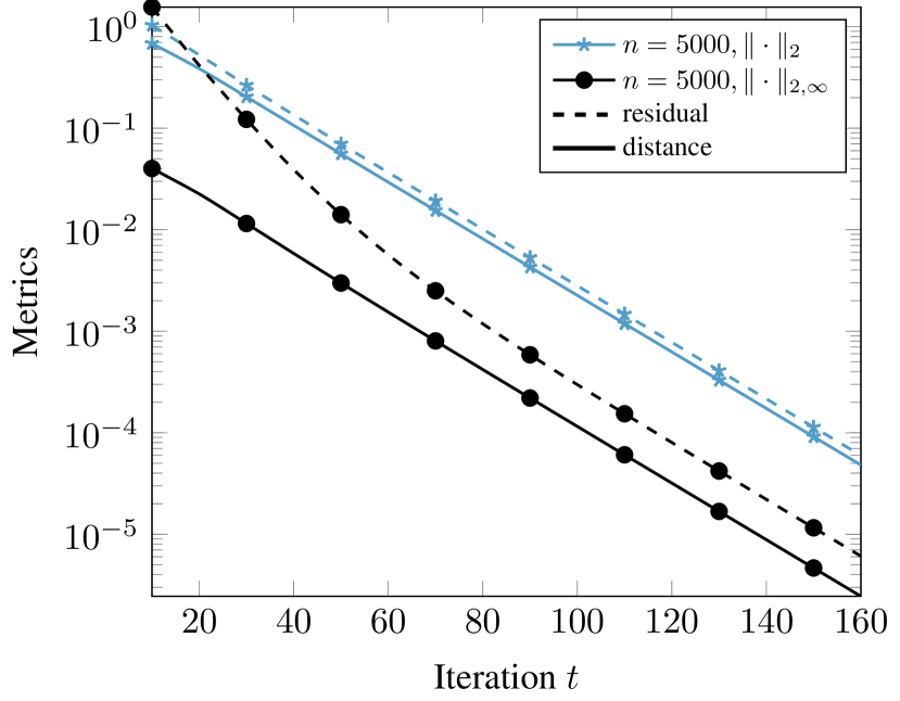
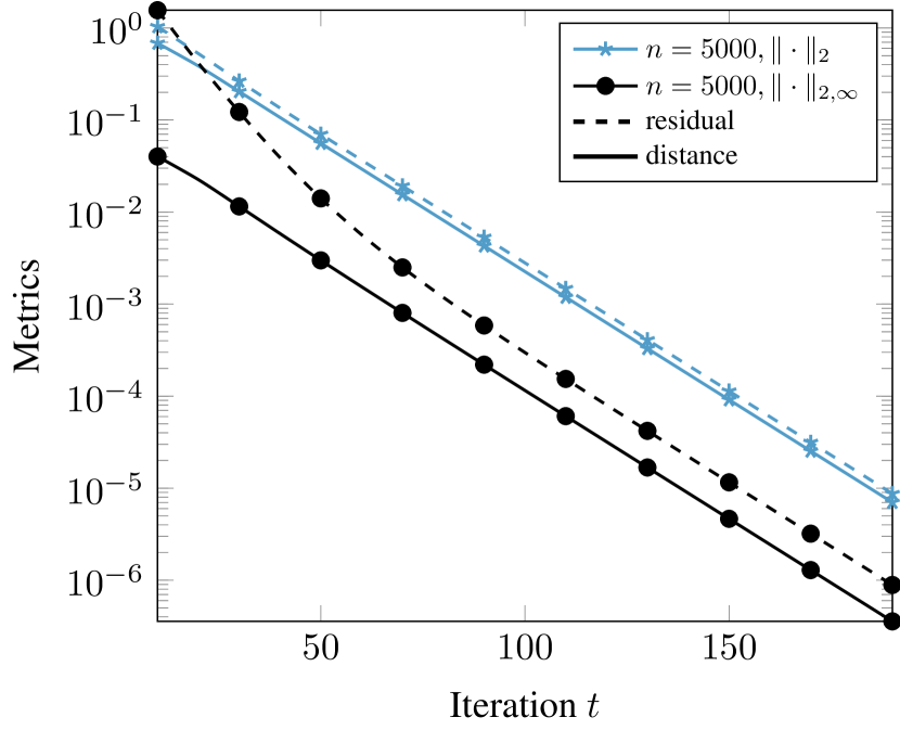
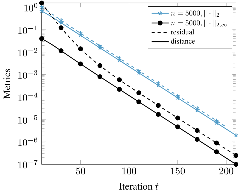
We compare distances and residuals for synthetic examples with $n=5000$ and $r=50$ and various stopping thresholds $\varepsilon$ for the residuals (Figure 1). Each plot in Figure 1 corresponds to a different matrix generated independently according to the aforementioned scheme. While the $\ell_{2}$ norm residual closely tracks the corresponding distance, the residual from Equation 10 overshoots by a small multiplicative factor, suggesting that the large constants in Proposition 3 may only be necessary in pathological cases and could be reduced in practice. Moreover, the $\ell_{2\to\infty}$ norm residual can substantially overestimate the actual distance in the first few iterations, as the estimate of Equation 10 depends on $Q_{t}Q_{t}^{\mathsf{T}}$ not being “too far” from $VV^{\mathsf{T}}$. The gap narrows after a few dozen iterations.

In addition, we examine the looseness of the bounds from Propositions 1 and 2 for the same experiment (Figure 2). We evaluate the following rates:

$$\begin{aligned} \mathsf{rate}_{1}(t)&:=\left(\frac{\lambda_{r+1}}{\lambda_{r}}\right)^{t}\cdot\frac{\mathrm{dist}_{2\to\infty}(Q_{0},V)}{\sqrt{1-d_{0}^{2}}},\quad\mathsf{rate}_{2}(t):=\text{ rate from~{}\lx@cref{creftypecap~refnum}{prop:2infnorm-convergence-single}},\\ \mathsf{rate}_{3}(t)&:=\text{ rate from~{}\lx@cref{creftypecap~refnum}{prop:2inf-convergence-general}},\quad\mathsf{rate}_{\textrm{naive}}(t):=\left(\frac{\lambda_{r+1}}{\lambda_{r}}\right)^{t}\frac{d_{0}}{\sqrt{1-d_{0}^{2}}}\end{aligned}$$ (11)

Here, $\mathsf{rate}_{1}$ is an idealized rate that mirrors classical convergence results for the $\ell_{2}$ norm [25, Theorem 8.2.2]; on the other hand, the naive rate just measures the $\ell_{2}$ subspace distance. In all the synthetic examples we generated, Assumption 1 was verified to hold with constant $C<2$ for all elapsed iterations $t$.

Figure 1: Distances (solid lines) and residuals (dashed lines) for synthetic examples with $r=50$ and target accuracies $\varepsilon=10^{-4}$ (left), $\varepsilon=10^{-5}$ (middle) and $\varepsilon=10^{-6}$ (right). Each plot corresponds to an independently generated synthetic example.

Figure 2: Distance (solid lines) and convergence rates from Equation 11 for matrix and subspace dimensions $(n,r)=(1000,10)$ (left); $(3500,15)$ (middle); and $(8000,20)$ (right). Our $\mathsf{rate}_{3}$ from Proposition 1 tracks the “idealized” rate $\mathsf{rate}_{1}$ closely in the synthetic data examples.

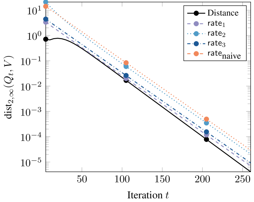
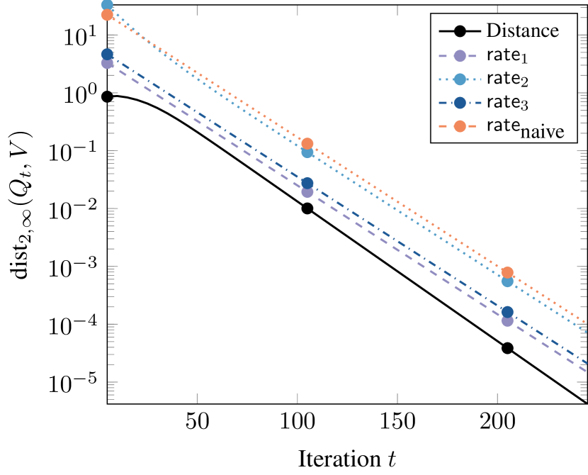
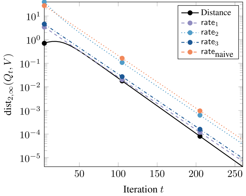
Remarkably, for a range of dimensions $n$ and $r$ we find that $\mathsf{rate}_{3}$ (which uses Proposition 1) closely tracks the “idealized” $\mathsf{rate}_{1}$ on these synthetic matrices (Figure 2). Also, $\mathsf{rate}_{2}$ (which uses Proposition 2) is a looser upper bound. This agrees with our theoretical analysis, as $\lambda_{r+2}$ is only moderately smaller than $\lambda_{r+1}$ in our synthetic matrix construction. Finally, as expected, the naive rate is the loosest bound.

Eigenvector centrality.

Next, we develop an experiment for network centrality, where the task is to measure the influence of nodes in a graph [43]. Each node is assigned a score, which is a function of the graph topology, and a typical underlying assumption is that a node with a high score contributes a larger influence to its adjacent ones. Here, we consider eigenvector centrality, which is one the standard measures in network science. Given a graph $G=(V,E)$; the eigenvector centrality score of a node $u$, $x_{u}>0$, is defined as a solution to the following equation:

$$x_{u}:=\frac{1}{\lambda}\sum_{v\in V}A_{uv}x_{v},\;A_{uv}:=\begin{cases}1,&\text{if $u$ links to $v$}\\ 0,&\text{otherwise}\end{cases},$$ (12)

where $\lambda$ is a proportionality constant. Here, node $u$’s scores depend linearly on all of its neighbors’ scores. Under the positivity requirement of $x_{u}$ and provided that the graph is connected and non-bipartite, rearranging and the Perron-Frobenius theorem show that $x=v_{1}$, the leading eigenvector of $A$ (up to scaling). To determine the most influential nodes, we are typically interested in the induced ordering of nodes and not the actual scores themselves. Therefore, the $\ell_{2\to\infty}$ distance, which measures $\left\|v_{1}-\hat{v}_{1}\right\|_{\infty}$, is more appropriate than $\left\|v_{1}-\hat{v}_{1}\right\|_{2}$ as a proxy for the quality of the estimate $\hat{v}_{1}$. To get a correct ranking result, it suffices to have $\left\|v_{1}-\hat{v}_{1}\right\|_{\infty}<(1/2)\cdot\min_{i,j}\left|v_{i}-v_{j}\right|$. On the other hand, $\left\|\hat{v}_{1}-v_{1}\right\|_{2}$ does not have an interpretable criterion.

We demonstrate the above principle by comparing two stopping criteria: the criterion from Equation 10 with a specified threshold $\varepsilon$ against the “naive” way of stopping when $\left\|A\hat{v}_{1}-\hat{\lambda}\hat{v}_{1}\right\|_{2}\leq\hat{\lambda}\varepsilon$, where $\hat{\lambda}$ is the current eigenvalue estimate, via the two following stopping times:

$$\begin{aligned} t_{\textrm{comp}}&:=\min\left\{t>0\ \middle|\ \mathsf{res}_{2\to\infty}(t)\leq\varepsilon\right\}\\ t_{\textrm{naive}}&:=\min\left\{t>0\ \middle|\ \left\|A\hat{V}_{:,j}-\hat{\lambda}_{j}\hat{V}_{:,j}\right\|\leq\varepsilon\hat{\lambda}_{j},\forall j\in\left\{1,\dots,r\right\}\right\}\end{aligned}.$$ (13)

For a user-specified tolerance $\varepsilon$, we expect that using our $\ell_{2\to\infty}$ error measurements and our corresponding stopping criteria will tell us that we can be confident in our solution much more quickly.

Table 1: Summary statistics of network datasets.

Dataset	Citation	# nodes	# edges
ca-HepPh	[34]	11204	117649
ca-AstroPh		17903	197031
gemsec-facebook-artist	[49]	50515	819306
com-DBLP	[58]	317080	1049866
com-LiveJournal		3997962	34681189

Figure 3: Ratio of the number of iterations needed to satisfy the two stopping criteria outlined in (13), for thresholds $\varepsilon=10^{-k}$, for computing eigenvector centrality to find the $\left\lfloor\sqrt{n}\right\rfloor$ most influential nodes (left) and computing the leading $r$ eigenvectors for spectral clustering (right). Our analysis and stopping criteria enable significantly fewer iterations.

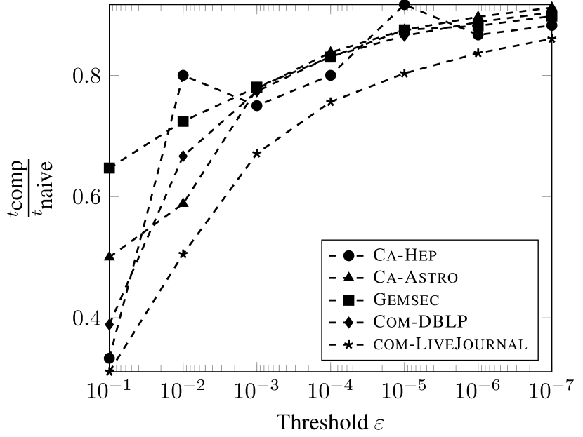
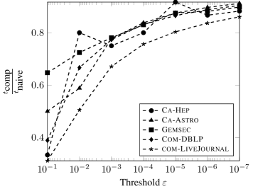
This is indeed the case — using our methodology provides a substantial reduction in computation time on a variety of real-world graphs, whose summary statistics are in Table 1. Figure 3 (left) shows the ratio between the two quantities $t_{\textrm{comp}}$ and $t_{\textrm{naive}}$, defined as in Equation 13. In the low-to-medium accuracy regimes, using our stopping method results in at least a 20–40% reduction in the number of iterations needed. In this regime, the ranking induced by the approximate eigenvector had typically already converged to the “true” ordering obtained by computing the eigenvector to machine precision.

Spectral clustering in graphs.

Another downstream task employing invariant subspaces is spectral clustering, which we study here as a way to partition a graph into well-separated “communities” or “clusters.” The standard pipeline is to compute the leading $r$-dimensional eigenspace of the normalized adjacency matrix, where $r$ is the desired number of clusters, The resulting eigenvector matrix provides an $r$-dimensional embedding for each node, which is subsequently fed to a point cloud clustering algorithm such as k-means [55]. For our experiment, we use the deterministic QR-based algorithm from [15] on the same set of real-world graphs that we used for eigenvector centrality.

In this setup, the eigenvectors (more carefully, a rotation of them) are approximate cluster indicators. Indeed, spectral clustering on graphs is often derived from a continuous relaxation of a combinatorial objective based on these indicators [55]. Thus, we are once again interpreting the eigenvectors entry-wise, and $\ell_{2\to\infty}$ error is a more sensible metric than $\ell_{2}$ error, This fact has been used to analyze random graph models with cluster structure [37].

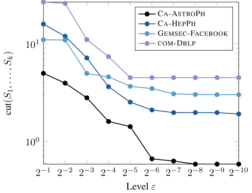
In the same manner as the eigenvector centrality experiment, we compare the ratio of iteration counts: $t_{\textrm{comp}}$ over $t_{\textrm{naive}}$, as defined in Equation 13 (Figure 3, right). In this case, we see even larger savings. For $\varepsilon$ around $10^{-2}$, our stopping criterion results in 70–80% savings in computation time. While this approximation level may seem crude at first, we can measure the performance of the algorithms in terms of the normalized cut metric, for which spectral clustering is a continuous relaxation [55]. We find that by the time we reach residual level $\varepsilon=10^{-2}$, the cut value found using the approximate subspace is essentially the same as the one using the subspace computed to numerical precision. Further details about the experiment are provided in the supplementary material.

Spectral bipartitioning and sweep cuts.

Another spectral method for finding clusters in graphs is spectral bipartitioning, which aims to find a single cluster of nodes $S$ with small conductance $\phi(S)$:

$$\phi(S):=\frac{\sum_{i\in S,j\notin S}A_{ij}}{\min(A(S),A(S^{c}))},\;A(S):=\sum_{i\in S}\sum_{j\in V}A_{ij}.$$

The conductance objective is a standard measure for identifying a good cluster of nodes [51, 35]: if $\phi(S)$ is small, there are not many edges leaving $S$ and there are many edges contained in $S$.

Minimizing $\phi(S)$ is NP-hard, but a spectral method using the eigenvector $v_{2}$ corresponding to the second largest eigenvalue of the normalized adjacency matrix, often called the Fiedler vector [22], provides guarantees. To find the a set with small conductance, the method uses the so-called “sweep cut”. After scaling $v_{2}$ by the inverse square root of degrees, we sort the nodes by their value in the eigenvector, and then consider the top-$k$ nodes as a candidate set $S$ for all values of $k$. The value of $k$ that gives the smallest conductance produces a set $S$ satisfying $\phi(S)\leq 2\sqrt{\min_{S^{\prime}}\phi(S^{\prime})}$, which is the celebrated Cheeger inequality [14].

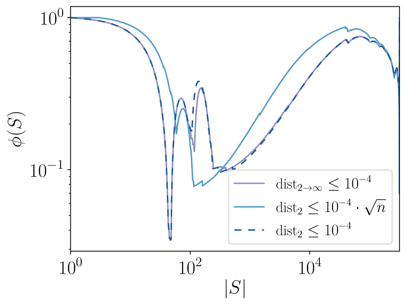
As in the case of eigenvector centrality, what matters is the ordering induced by the eigenvector, making a $\ell_{2\to\infty}$ stopping criterion more appropriate. As a heuristic, one might consider just making $\ell_{2}$ tolerance larger (by the norm equivalence factor) using a level of $\varepsilon$ for the $\ell_{2\to\infty}$ distance and $\varepsilon\cdot\sqrt{n}$ for the $\ell_{2}$ distance. However, this can substantially reduce the solution quality. This is illustrated in Figure 4, where we plot the conductance values obtained in the sweep cut as a function of the size of the set on com-Dblp. This is a sweep cut approximation of a network community profile plot [8, 35], which visualizes cluster structure at different scales. Using the naive $\ell_{2}$ stopping criterion provides the same solution quality but requires more iterations. In the case of $\varepsilon=10^{-4}$ in Figure 4, our methods produce 20% computational savings. Finally, the heuristic $\varepsilon\cdot\sqrt{n}$ tolerance for the $\ell_{2}$ stopping criterion produces a cruder solution and finds a set with larger conductance.

Figure 4: Sweep cut profile (cut conductance vs. cardinality) for com-Dblp. For a fixed $\varepsilon$, our $\ell_{2\to\infty}$ stopping criterion leads to faster convergence. Increasing the tolerance for $\ell_{2}$ by the norm equivalence factor produces lower-quality solutions. Here $t_{\textrm{comp}}=1135$ vs. $t_{\textrm{naive}}=1378$ iterations.

5 Conclusions

The broad applicability of spectral methods, coupled with the prevalence of entry-wise / row-wise interpretations of eigenspaces strongly motivates imbuing our computational methods with appropriate stopping criteria. Our theoretical results demonstrate just how much smaller the $\left\|\cdot\right\|_{2\to\infty}$ subspace distance can be than traditional measures, an observation supported by experiment. In fact, the accuracy with which we compute eigenvectors can have a non-trivial impact on downstream applications —  if we would like use fewer iterations to save time we must do so carefully, and our new stopping criterion provides an easy to implement way to do this that comes at essentially no cost and with strong guarantees.

From a theoretical perspective, it may seem sufficient to use norm equivalence and simply appeal to spectral norm convergence, which can incur an extra $\mathcal{O}(\log n)$ factor at most when computing subspaces. However, such reasoning only applies to the very-high-accuracy regime. As demonstrated by our experiments, moderate levels of accuracy often suffice for downstream applications, in which case our stopping criterion allows for highly nontrivial computational savings (up to 70% fewer iterations).

Broader impact

Due to the pervasiveness of spectral methods in machine learning and data mining, our results may be embedded in applications having a wide range of ethical and societal consequences. Indeed, given the fact that eigensolvers are typically used as linear algebra primitives, our work “inherits” the ethical and societal consequences of the context in which its results are applied, as well as the potential implications of “failure” (e.g., if our stopping criterion severely underestimates the true approximation error).

Appendix A Additional experimental details

This section documents hyperparameters and other design choices used to run the experiments in Section 4 of the main paper.

A.1 Eigenvector centrality

In all eigenvector centrality experiments, we isolate the largest connected component of the input graph and work exclusively within that component. We work with the unnormalized version of the adjacency matrix, since the normalized version admits the vector $d^{1/2}:=\mathrm{diag}(\sqrt{d_{1}},\dots,\sqrt{d_{n}})$, where $d_{i}$ is the degree of the $i^{\textrm{th}}$ node, as its principal eigenvector.

We initialize the estimate $\hat{v}_{1}:=\frac{1}{\sqrt{n}}\bm{1}$, the normalized all-ones vector. In the absence of incoherence, we use the expression of Equation 10 in the main text to evaluate the $\ell_{2\to\infty}$ stopping criterion, and set $\mathsf{gap}=\lambda_{1}-\lambda_{2}$ using the values returned by Arpack, to ensure a fair comparison. At each step of the iterative method, we multiply with $\pm 1$ accordingly, to ensure that all entries of the approximate eigenvector are positive.

Ranking distance.

To measure the “distance” between the approximate ranking produced by our eigenvector estimate, we employ Kendall’s $\tau$ criterion [29]. In particular, we define

$$\mathrm{dist}_{\tau}(v_{1},\hat{v}_{1}):=\frac{1-\tau(v_{1},\hat{v}_{1})}{2}$$ (14)

to compare the rankings induced by $v_{1}$ and $\hat{v}_{1}$. It is easy to verify that when the rankings are identical, $\mathrm{dist}_{\tau}=0$, and when the rankings are the most dissimilar, $\mathrm{dist}_{\tau}=1$, since $\tau(v_{1},\hat{v}_{1})\in[-1,1]$.

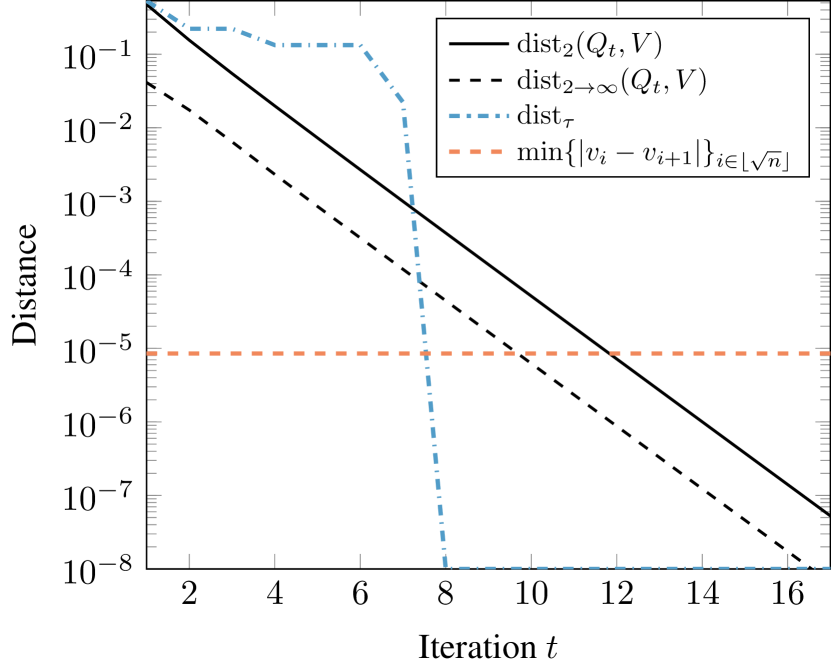
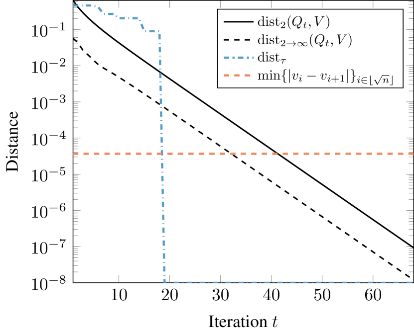
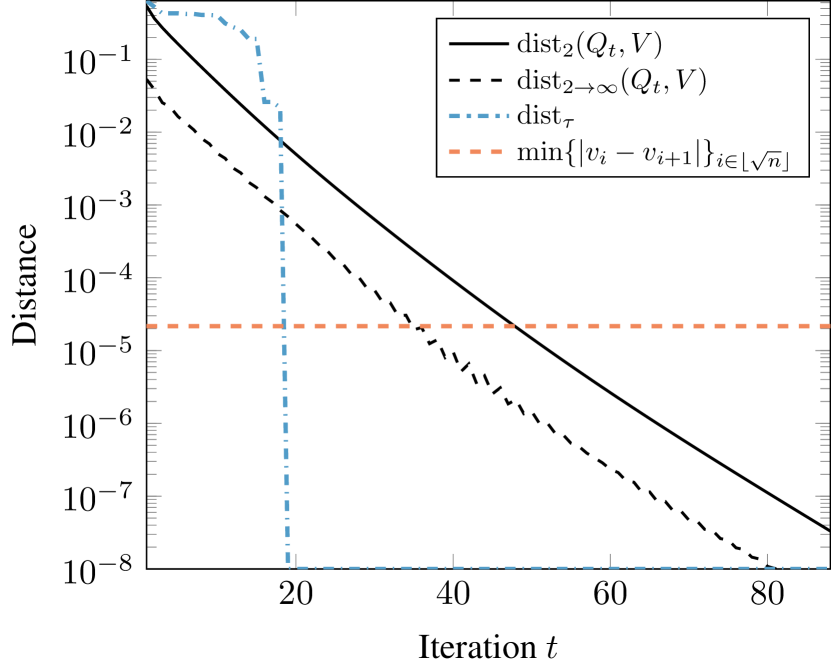
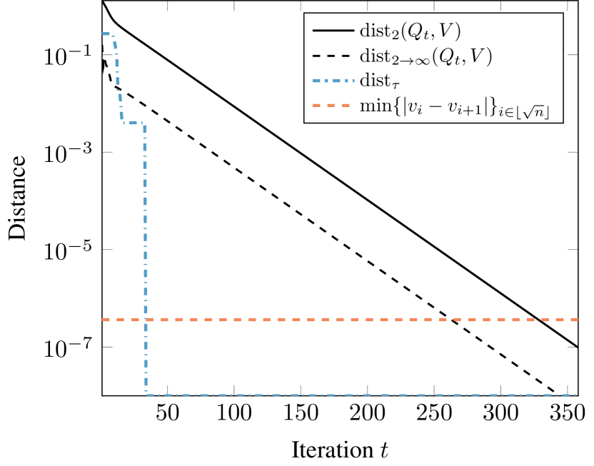
The convergence plots for $4$ datasets, where we depict the “oracle” $\ell_{2}$ and $\ell_{2\to\infty}$ subspace distances as well as $\mathrm{dist}_{\tau}$ as a function of the iteration index $t$, are shown in Figure 5. In all cases, we identify the correct ranking when the residual is in the low-to-moderate accuracy regime ($\varepsilon\leq 10^{-4}$).

Figure 5: Distance plots for $4$ datasets, for which the top $\left\lfloor\sqrt{n}\right\rfloor$ nodes are being ranked. From left to right: ca-HepPh, ca-AstroPh (top), Gemsec, com-LiveJournal (bottom).

A.2 Spectral clustering

In this section, we describe the methodology used for the spectral clustering experiments in the main text. We opt to use the Algorithm of [15] which is based on the column-pivoted QR decomposition of an appropriately defined matrix. For completeness, the full algorithm is listed in Algorithm 2. Since the algorithm is deterministic, we do not have to worry about randomness pertaining to initialization (e.g. as in kmeans++), and only run the experiment once for each configuration of parameters.

Algorithm 2 CPQR-based clustering

1:Input: invariant subspace $V_{k}\in\mathbb{R}^{n\times r}$

2:Compute the CPQR factorization

$$V_{k}^{\top}\Pi=QR,$$

where $\Pi$ is a column selection matrix.

3:Let $\mathcal{C}$ denote the first $k$ columns identified by $\Pi$.

4:Compute the polar factorization

$$(V_{k}^{\top})_{:,\mathcal{C}}=UH.$$

5:for $j\in[n]$ do

6:     assign node $j$ to cluster

$$C_{j}:=\operatorname*{argmax}_{i}\left|(UV_{k}^{\top})_{i,j}\right|$$

7:end for

For all the datasets involved, we hand-pick the target number of clusters $r$ by inspecting the successive ratios of the leading few eigenvalues and setting $r$ so that the ratio $\frac{\lambda_{r+1}}{\lambda_{r}}$ is small, but also taking into account the fact that we don’t want $r$ to be too small. Additionally, we use the regularized version of the normalized adjacency matrix $A_{\rho}$ [2], which augments the adjacency and degree matrices $A,D$ using a regularization parameter $\rho$:

$$A_{\rho}:=A+\frac{\rho}{n}\bm{1}\bm{1}^{\top},\quad D_{\rho}:=D+\rho$$ (15)

Following standard practice [47, 59], we set $\rho$ equal to a constant which is near the average degree of the graph and then perform the eigendecomposition of

$$\tilde{A}_{\rho}=D_{\rho}^{-1/2}A_{\rho}D_{\rho}^{-1/2}+I,$$

shifting by $+I$ to ensure that the algebraically largest eigenvalues are also the largest in magnitude, in order for subspace iteration to be applicable. We summarize the hyperparameter choices for each dataset in Table 2.

Table 2: Parameters for spectral clustering

Dataset	$r$	$\tau$
ca-HepPh	$17$	$1.0$
ca-AstroPh	6	$1.0$
GemSec	12	1.0
Dblp	28	5.0

Figure 6: Ratio of iterations required to satisfy $\mathsf{res}_{2\to\infty}(t)\leq\varepsilon$ ($t_{\textrm{comp}}$) over number of iterations required to satisfy $\mathsf{res}_{2}(t)\leq\varepsilon$ ($t_{\textrm{naive}}$) in eigenvector centrality computations.

To evaluate the quality of a given clustering assignment, we use the normalized cut metric. Specifically, given a vertex set $V$ and a partition $(S,S^{c})$ such that $V=S\cup S^{c}$, we define the conductance of the cut induced by $S$ as

$$\phi(S):=\frac{\sum_{i\in S,j\notin S}A_{ij}}{A(S)}\quad A(S):=\sum_{i\in S}\sum_{j\in V}A_{ij}$$ (16)

Note that in (16), $A$ refers to the unnormalized adjacency matrix, with $A_{ij}=A_{ji}=1$ if the edge $(i,j)$ exists in the graph, and $0$ otherwise. Then any clustering assignment with $k$ clusters induces $k$ partitions $\left\{(S_{k},S_{k}^{c})\right\}$, for which the normalized cut metric is defined as

$$\textrm{ncut}(S_{1},\dots,S_{k}):=\frac{1}{2}\sum_{i=1}^{k}\phi(S_{k}).$$ (17)

Figure 8 depicts the value of $\textrm{ncut}(S_{1},\dots,S_{k})$ when the input to Algorithm 2 is computed using subspace iteration, using the proposed stopping criterion, for different levels $\varepsilon$.

Figure 7: Value of $\textrm{ncut}(S_{1},\dots,S_{k})$ for various datasets, with $\hat{V}_{k}$ computed using subspace iteration until the residual drops below level $\varepsilon$, for different values of $\varepsilon$. In all cases, the metric stabilizes while in the low accuracy regime ($\varepsilon\approx 10^{-2}$). Dashed lines indicate the value of $\textrm{ncut}(S_{1},\dots,S_{k})$ found by computing the subspace to machine accuracy.

Figure 8: Ratio of iterations required to satisfy $\mathsf{res}_{2\to\infty}(t)\leq\varepsilon$ ($t_{\textrm{comp}}$) over number of iterations required to satisfy $\mathsf{res}_{2}(t)\leq\varepsilon$ ($t_{\textrm{naive}}$) in the spectral clustering setting, showing computational gains of over $50\%$.

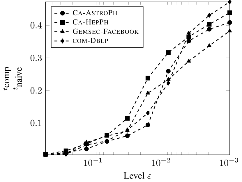
Having established that low-to-moderate accuracy is sufficient for this problem, we plot the ratio of $t_{\textrm{comp}}$ over $t_{\textrm{naive}}$; the former is the number of iterations required to satisfy $\mathsf{res}_{2\to\infty}(t)\leq\varepsilon$, while the latter is the number of iterations required to satisfy $\mathsf{res}_{2}(t):=\left\|A\hat{v}_{t}-\hat{\lambda}_{t}\hat{v}_{t}\right\|_{2}\leq\hat{\lambda}_{t}\varepsilon$. We observe computational gains of over $50\%$ in all cases.

A.3 Empirically verifying Assumption 1

We verified that Assumption 1 from the main text holds in practice for the real world datasets used in the experimental section. Recall that the assumption asks that the matrix $A=V\Lambda V^{\mathsf{T}}+V_{\perp}\Lambda_{\perp}V_{\perp}^{\mathsf{T}}$ satisfies:

$$\left\|V_{\perp}\Lambda_{\perp}^{t}V_{\perp}^{\mathsf{T}}\right\|_{\infty}\leq C\cdot\left\|\Lambda_{\perp}^{t}\right\|_{2}\cdot\left\|V_{\perp}V_{\perp}^{\mathsf{T}}\right\|_{\infty},$$ (18)

where $C$ is a constant independent of $n$, for all $t\in\mathbb{N}$. First, observe that for our purposes, we only want this assumption to hold for all $t$ until our iterative algorithm stops. Since all our experiments take fewer than $T=1500$ iterations to run, we opt to verify (18) for $t\in\left\{1,\dots,T\right\}$. We first rephrase the assumption as

$$\left\|A^{t}-V\Lambda^{t}V^{\mathsf{T}}\right\|_{\infty}\leq C\cdot\lambda^{t}_{\max}(\Lambda_{\perp})\cdot\left\|I-VV^{\mathsf{T}}\right\|_{\infty},$$ (19)

which can be checked after computing the top $r+1$ eigenvectors and eigenvalues of $A$; these were computed to machine precision using eigs. For $t=1$ up to $t=T$, we checked (19) exhaustively, and output

$$C:=\sup_{t\in\left\{1,\dots,T\right\}}\left\{\frac{\left\|A^{t}-V\Lambda^{t}V^{\mathsf{T}}\right\|_{\infty}}{\lambda_{r+1}^{t}\left\|I-VV^{\mathsf{T}}\right\|_{\infty}}\right\}$$

In all cases, we end up with a constant $C<2$.

Appendix B Auxiliary results

Lemma 2 (Incoherence).

Consider a subspace $\mathcal{V}$ of dimension $r$ and a matrix $V\in\mathbb{O}_{n,r}$ whose columns span $\mathcal{V}$. If $\mu$ is the coherence of $V$, i.e. $\left\|V\right\|_{2\to\infty}\leq\mu\sqrt{\frac{r}{n}}$, then for its complementary subspace $\mathcal{V}_{\perp}$ it holds that

$$\left\|V_{\perp}{V_{\perp}}^{\mathsf{T}}\right\|_{\infty}\leq(1+\mu\sqrt{r}).$$

Proof.

Observe that $\left\|A\right\|_{\infty}\leq\sqrt{n}\left\|A\right\|_{2\to\infty}$, thus

$$\left\|V_{\perp}{V_{\perp}}^{\mathsf{T}}\right\|_{\infty} =\left\|I-VV^{\mathsf{T}}\right\|_{\infty}\leq 1+\left\|VV^{\mathsf{T}}\right\|_{\infty}\leq 1+\sqrt{n}\left\|VV^{\mathsf{T}}\right\|_{2\to\infty}\leq 1+\sqrt{n}\mu\sqrt{\nicefrac{{r}}{{n}}}.$$

∎

The next theorem, originally stated without assuming symmetry, is adapted for the case of a symmetric initial matrix.

Theorem 1 (Theorem 5.1 in [16]).

Suppose $\tilde{A}=A+E$ with $A$ symmetric, having eigenvalue decomposition $A=V\Lambda V^{\mathsf{T}}+V_{\perp}\Lambda_{\perp}V_{\perp}^{\mathsf{T}},$ where $V\in\mathbb{R}^{n\times r},V_{\perp}\in\mathbb{R}^{n\times(n-r)}$ have orthonormal columns. Moreover, let $\mathsf{gap}:=\min\left\{\lambda_{r}-\lambda_{r+1},\mathsf{sep}_{(2,\infty),V_{\perp}}(\Lambda,V_{\perp}\Lambda_{\perp}{V_{\perp}}^{\mathsf{T}})\right\}$. If $\left\|E\right\|_{2}\leq\frac{\mathsf{gap}}{5}$, then the leading invariant subspace of $\tilde{A}$, $\tilde{V}$, satisfies

$$\begin{aligned} \inf_{O\in\mathbb{O}_{r}}\left\|\tilde{V}-VO\right\|_{2\to\infty}&\leq 8\left\|V\right\|_{2\to\infty}\left(\frac{\left\|E\right\|_{2}}{\lambda_{r}-\lambda_{r+1}}\right)^{2}+\frac{2\left\|V_{\perp}{V_{\perp}}^{\mathsf{T}}EV\right\|_{2\to\infty}}{\mathsf{gap}}\\ &+\frac{4\left\|V_{\perp}{V_{\perp}}^{\mathsf{T}}E\right\|_{2\to\infty}\left\|E\right\|_{2}}{\mathsf{gap}\cdot(\lambda_{r}-\lambda_{r+1})}.\end{aligned}$$ (20)

Lemma 3 ([11]).

We have

$$\left\|AB\right\|_{2\to\infty} \leq\left\|A\right\|_{2\to\infty}\left\|B\right\|_{2}$$ (21)

$$\left\|AB\right\|_{2\to\infty} \leq\left\|A\right\|_{\infty}\left\|B\right\|_{2\to\infty}$$ (22)

Moreover, for any matrix $V$ with orthonormal columns, it holds that

$$\left\|AV^{\mathsf{T}}\right\|_{2\to\infty}=\left\|A\right\|_{2\to\infty}.$$ (23)

We also prove the following claim, which is used throughout the proof of Proposition 1 in the next section.

Lemma 4.

We have $\inf_{Z\in\mathbb{O}_{r}}\left\|\tilde{V}-VZ\right\|_{2}\leq\sqrt{2}\mathrm{dist}_{2}(V,\tilde{V})$.

Proof.

Recall the solution of the orthogonal Procrustes problem, given by the SVD of $V^{\mathsf{T}}\tilde{V}$, $U\Sigma W^{\mathsf{T}}$. Since $UW^{\mathsf{T}}\in\mathbb{O}_{r}$, with $U^{\mathsf{T}}U=UU^{\mathsf{T}}=W^{\mathsf{T}}W=WW^{\mathsf{T}}=I_{r}$, we have

$$\inf_{Z\in\mathbb{O}_{r}}\left\|\tilde{V}-VZ\right\|_{2} \leq\left\|\tilde{V}-VUW^{\mathsf{T}}\right\|_{2}=\sqrt{\sup_{x}\left\langle x,(\tilde{V}-VUW^{\mathsf{T}})^{\mathsf{T}}(\tilde{V}-VUW^{\mathsf{T}})x\right\rangle}$$ (24)

$$=\sqrt{\sup_{x}\left\langle x,(I-\tilde{V}^{\mathsf{T}}VUW^{\mathsf{T}}-WU^{\mathsf{T}}V^{\mathsf{T}}\tilde{V}+I)x\right\rangle}$$ (25)

$$\overset{(\sharp)}{=}\sqrt{\sup_{x}\left\langle x,2(I-W\Sigma W^{\mathsf{T}})x\right\rangle}=\sqrt{2\left\|I-W\Sigma W^{\mathsf{T}}\right\|_{2}}$$ (26)

$$=\sqrt{2}\sqrt{\left\|I-\Sigma\right\|_{2}}=\sqrt{2}\sqrt{1-\sigma_{r}(V^{\mathsf{T}}\tilde{V})}$$ (27)

$$\overset{(\natural)}{\leq}\sqrt{2}\sqrt{1-\sigma_{r}^{2}(V^{\mathsf{T}}\tilde{V})}=\sqrt{2}\left\|V^{\mathsf{T}}\tilde{V}\right\|_{2},$$ (28)

where $(\sharp)$ follows after replacing $V^{\mathsf{T}}\tilde{V}=U\Sigma W^{\mathsf{T}}$ in the expression and gathering terms, while $(\natural)$ simply uses the fact that $\sigma_{r}(V^{\mathsf{T}}\tilde{V})\leq 1$ to upper bound the expression inside the square root. Finally, we use the fact that:

$$1-\sigma^{2}_{\min}(V^{\mathsf{T}}\tilde{V})=\left\|V_{\perp}^{\mathsf{T}}\tilde{V}\right\|_{2}^{2}=\mathrm{dist}_{2}^{2}(V,\tilde{V}).$$

∎

Appendix C Omitted proofs

C.1 Proof of Proposition 1

Starting with the definition of the $2\to\infty$ distance, we have

$$\mathrm{dist}_{2\to\infty}(Q_{t},V) =\inf_{Z\in\mathbb{O}_{r}}\left\|Q_{t}-VZ\right\|_{2\to\infty}=\inf_{Z\in\mathbb{O}_{r}}\left\|(VV^{\mathsf{T}}+V_{\perp}V_{\perp}^{\mathsf{T}})(Q_{t}-VZ)\right\|_{2\to\infty}$$ (29)

$$\overset{(\sharp)}{\leq}\sqrt{2}\left\|VV^{\mathsf{T}}\right\|_{2\to\infty}\mathrm{dist}_{2}(Q_{t},V)+\left\|V_{\perp}V_{\perp}^{\mathsf{T}}(Q_{t}-VZ)\right\|_{2\to\infty}$$ (30)

where ($\sharp$) follows from Lemma 3 and the fact that $\inf_{Z\in\mathbb{O}_{r}}\left\|Q_{t}-VZ\right\|_{2}\leq\sqrt{2}\mathrm{dist}_{2}(Q_{t},V)$. At this point, note that standard convergence results [50, 25] state that

$$\mathrm{dist}_{2}(Q_{t},V)\leq\left(\frac{\lambda_{r+1}}{\lambda_{r}}\right)^{t}\frac{d_{0}}{\sqrt{1-d_{0}^{2}}},$$

and additionally $\left\|VV^{\mathsf{T}}\right\|_{2\to\infty}\leq\mu\sqrt{\frac{r}{n}}$, where $\mu$ is the coherence of $V$.

For the remainder, let us first recall a fact from the analysis of subspace iteration; the $t^{\text{th}}$ iterate $Q_{t}$ satisfies

$$Q_{t}R_{t} =A^{t}V^{(0)},\;\text{ with $R_{t}$ invertible}\quad\Rightarrow\quad V_{\perp}^{\mathsf{T}}Q_{t}=V_{\perp}^{\mathsf{T}}A^{t}V^{(0)}R_{t}^{-1}=\Lambda_{\perp}^{t}V_{\perp}^{\mathsf{T}}V^{(0)}R_{t}^{-1}.$$ (31)

Then, notice that $V_{\perp}^{\mathsf{T}}V=0$ and therefore we can rewrite the second term in (30) as

$$\left\|V_{\perp}V_{\perp}^{\mathsf{T}}Q_{t}\right\|_{2\to\infty} \overset{(*)}{=}\left\|V_{\perp}\Lambda_{\perp}^{t}V_{\perp}^{\mathsf{T}}Q_{0}R_{t}^{-1}\right\|_{2\to\infty}\overset{(\flat)}{=}\inf_{Z\in\mathbb{O}_{r}}\left\|V_{\perp}\Lambda_{\perp}^{t}V_{\perp}^{\mathsf{T}}(Q_{0}-VZ)R_{t}^{-1}\right\|_{2\to\infty}$$ (32)

$$\overset{(\natural)}{\leq}\inf_{Z\in\mathbb{O}_{r}}C\left\|V_{\perp}V_{\perp}^{\mathsf{T}}\right\|_{\infty}\lambda_{r+1}^{t}\left\|(Q_{0}-VZ)R_{t}^{-1}\right\|_{2\to\infty}$$ (33)

$$\leq C\left\|V_{\perp}V_{\perp}^{\mathsf{T}}\right\|_{\infty}\lambda_{r+1}^{t}\underbrace{\inf_{Z\in\mathbb{O}_{r}}\left\|Q_{0}-VZ\right\|_{2\to\infty}}_{=\mathrm{dist}_{2\to\infty}(Q_{0},V)}\left\|R_{t}^{-1}\right\|_{2}$$ (34)

where $(*)$ follows from Equation 31, $(\flat)$ holds since we can reintroduce $VZ$ for any $Z$, as $V_{\perp}^{\mathsf{T}}V=0$, $(\natural)$ holds after combining Equation 22 and Assumption 1 from the main text, and the last inequality is Equation 21. Notice that $\left\|R_{t}^{-1}\right\|_{2}=\frac{1}{\sqrt{1-d_{0}^{2}}}\lambda_{r}^{-t},$ by tracing the proof of [25, Theorem 8.2.2]. Finally, by Lemma 2, $\left\|V_{\perp}V_{\perp}^{\mathsf{T}}\right\|_{\infty}\leq 1+\mu\sqrt{r}$. ∎

C.2 Proof of Proposition 2

For simplicity, let us define $\tilde{V}:=\begin{bmatrix}V&v_{r+1}\end{bmatrix}\in\mathbb{R}^{n\times(r+1)}$ and $\tilde{V}_{\perp}$ for the remaining $n-r-1$ eigenvectors forming a basis of $\mathbb{R}^{n}$. Similarly, let $\tilde{\Lambda}_{\perp}=\mathrm{diag}(\lambda_{r+2},\dots,\lambda_{n})$. Starting with the definition of the $2\to\infty$ distance, we have

$$\begin{aligned} \mathrm{dist}_{2\to\infty}(Q_{t},V)&=\inf_{Z\in\mathbb{O}_{r}}\left\|Q_{t}-VZ\right\|_{2\to\infty}=\inf_{Z\in\mathbb{O}_{r}}\left\|(VV^{\mathsf{T}}+V_{\perp}V_{\perp}^{\mathsf{T}})(Q_{t}-VZ)\right\|_{2\to\infty}\\ &\overset{(\sharp)}{\leq}\sqrt{2}\left\|VV^{\mathsf{T}}\right\|_{2\to\infty}\mathrm{dist}_{2}(Q_{t},V)+\left\|V_{\perp}V_{\perp}^{\mathsf{T}}(Q_{t}-VZ)\right\|_{2\to\infty}\end{aligned},$$ (35)

where ($\sharp$) follows from Lemma 3 in the main text and the fact that $\inf_{Z\in\mathbb{O}_{r}}\left\|Q_{t}-VZ\right\|_{2}\leq\sqrt{2}\mathrm{dist}_{2}(Q_{t},V)$. Now we may rewrite the second term as

$$\begin{aligned} \left\|(v_{r+1}v_{r+1}^{\mathsf{T}}+\tilde{V}_{\perp}\tilde{V}_{\perp}^{\mathsf{T}})Q_{t}\right\|_{2\to\infty}&\leq\left\|v_{r+1}v_{r+1}^{\mathsf{T}}Q_{t}\right\|_{2\to\infty}+\left\|\tilde{V}_{\perp}\tilde{V}_{\perp}^{\mathsf{T}}Q_{t}\right\|_{2\to\infty}\\ &=\left\|v_{r+1}\lambda_{r+1}^{t}v_{r+1}^{\mathsf{T}}Q_{0}R_{t}^{-1}\right\|_{2\to\infty}+\left\|\tilde{V}_{\perp}\tilde{\Lambda}^{t}_{\perp}\tilde{V}_{\perp}^{\mathsf{T}}Q_{0}R_{t}^{-1}\right\|_{2\to\infty}.\end{aligned}$$ (36)

Pulling $\lambda_{r+1}^{t}$ out of the first norm in (36) yields

$$\left\|v_{r+1}v_{r+1}^{\mathsf{T}}(Q_{0}-VZ_{\star})\right\|_{2\to\infty}\left\|R_{t}^{-1}\right\|_{2}\leq\left\|v_{r+1}v_{r+1}^{\mathsf{T}}\right\|_{\infty}\mathrm{dist}_{2\to\infty}(Q_{0},V)\cdot\frac{\lambda_{r}^{-t}}{\sqrt{1-d_{0}^{2}}},$$

after using Lemma 3 and the fact that $\left\|R_{t}^{-1}\right\|_{2}\leq\frac{\lambda_{r}^{-t}}{\sqrt{1-d_{0}^{2}}}$, while the second norm in (36) can be upper bounded by

$$\left\|\cancel{\tilde{V}_{\perp}}\tilde{\Lambda}^{t}_{\perp}\right\|_{2}\left\|\tilde{V}_{\perp}^{\mathsf{T}}Q_{-}\right\|_{2}\left\|R_{t}^{-1}\right\|_{2}=\left(\frac{\lambda_{r+2}}{\lambda_{r}}\right)^{t}\frac{\mathrm{dist}_{2}(Q_{0},\tilde{V})}{\sqrt{1-d_{0}^{2}}},$$

but as the respective subspaces satisfy $\mathcal{V}\subset\tilde{\mathcal{V}}$ we have $\mathrm{dist}_{2}(Q_{0},\tilde{V})\leq\mathrm{dist}_{2}(Q_{0},V)$. Combining all the ingredients above completes the proof. ∎

C.3 Proof of Proposition 3

The condition on $\left\|E\right\|_{2}$ combined with the assumption that $Q$ is the leading invariant subspace of the perturbed matrix $A-EQ^{\mathsf{T}}$ allows us to apply Theorem 1 for the perturbation $EQ^{\mathsf{T}}$, from which we deduce that the approximate eigenvector matrix $V$ satisfies

$$\mathrm{dist}_{2\to\infty}(Q,V)\leq 8\left\|V\right\|_{2\to\infty}\left(\frac{\left\|E\right\|_{2}}{\lambda_{r}-\lambda_{r+1}}\right)^{2}+2\frac{\left\|V_{\perp}V_{\perp}^{\mathsf{T}}EQ^{\mathsf{T}}V\right\|_{2\to\infty}}{\mathsf{gap}}+4\frac{\left\|V_{\perp}V_{\perp}^{\mathsf{T}}E\right\|_{2\to\infty}\left\|E\right\|_{2}}{\mathsf{gap}\cdot(\lambda_{r}-\lambda_{r+1})}$$

with the appropriate definition of $\mathsf{gap}$. Using Lemma 3, we can upper bound the terms above as

$$\left\|V_{\perp}V_{\perp}^{\mathsf{T}}EQ^{\mathsf{T}}V\right\|_{2\to\infty}\leq\left\|V_{\perp}V_{\perp}^{\mathsf{T}}\right\|_{\infty}\left\|EQ^{\mathsf{T}}V\right\|_{2\to\infty}\leq\left\|V_{\perp}V_{\perp}^{\mathsf{T}}\right\|_{\infty}\left\|E\right\|_{2\to\infty}\underbrace{\left\|Q^{\mathsf{T}}V\right\|_{2}}_{\leq 1},$$ (37)

and similarly for the term $\left\|V_{\perp}V_{\perp}^{\mathsf{T}}E\right\|_{2\to\infty}$. ∎

Appendix D Miscellanea

D.1 Eigenvalue localization issues

We briefly address the issue of when we can safely assume that the approximate invariant subspace $Q$, utilized in Proposition 3, is the leading invariant subspace of the perturbed matrix $A-EQ^{\mathsf{T}}$. While the matrix of Ritz values, $S$, is within $\sqrt{2}\left\|E\right\|_{2}$ distance of a set of $r$ eigenvalues of $A$, we do not know whether or not these eigenvalues correspond to the largest (in magnitude) eigenvalues of $A-EQ^{\mathsf{T}}$.

In this case, one has to appeal to algorithm-specific arguments. Recall that $A$ has spectral decomposition $A=V\Lambda V^{\mathsf{T}}+V_{\perp}\Lambda_{\perp}V_{\perp}^{\mathsf{T}},$ where $\Lambda$ contains the dominant $r$ eigenvalues. Let $Q_{\perp}\in\mathbb{O}_{n,n-r}$ be orthogonal to the approximate eigenvector matrix $Q\in\mathbb{O}_{n,r}$. Then the following

$$\begin{bmatrix}Q^{\mathsf{T}}\\ Q_{\perp}^{\mathsf{T}}\end{bmatrix}(A-EQ^{\mathsf{T}})\begin{bmatrix}Q&Q_{\perp}\end{bmatrix} =\begin{bmatrix}S&Q^{\mathsf{T}}(A-EQ^{\mathsf{T}})Q_{\perp}\\ Q_{\perp}^{\mathsf{T}}QS&Q_{\perp}^{\mathsf{T}}(A-EQ^{\mathsf{T}})Q_{\perp}\end{bmatrix}=\begin{bmatrix}S&Q^{\mathsf{T}}AQ_{\perp}\\ \bm{0}&Q_{\perp}^{\mathsf{T}}AQ_{\perp}\end{bmatrix}$$

is a Schur decomposition of $A-EQ^{\mathsf{T}}$, with its eigenvalues being the union $S\cup\Lambda(Q_{\perp}^{\mathsf{T}}AQ_{\perp})$ – the objective becomes showing that $\left\|\Lambda(Q_{\perp}^{\mathsf{T}}AQ_{\perp})\right\|_{2}$ is sufficiently small, after enough progress of the algorithm. By the variational characterization of singular values for symmetric matrices, we have

$$\left\|Q_{\perp}^{\mathsf{T}}AQ_{\perp}\right\|_{2} =\sup_{x\in\mathbb{S}^{n-1}}\left|\left\langle x,Q_{\perp}^{\mathsf{T}}AQ_{\perp}x\right\rangle\right|$$ (38)

$$=\sup_{x\in\mathbb{S}^{n-1}}\left|\left\langle x,Q_{\perp}^{\mathsf{T}}V\Lambda V^{\mathsf{T}}Q_{\perp}x\right\rangle+\left\langle x,Q_{\perp}^{\mathsf{T}}V_{\perp}\Lambda_{\perp}V_{\perp}^{\mathsf{T}}Q_{\perp}x\right\rangle\right|$$ (39)

$$\overset{(*)}{\leq}\left|\lambda_{1}(A)\right|\left\|Q_{\perp}^{\mathsf{T}}V\right\|_{2}^{2}+\left|\lambda_{r+1}(A)\right|\cancelto{\leq 1}{\left\|Q_{\perp}^{\mathsf{T}}V_{\perp}\right\|}$$ (40)

Therefore, as soon as $\mathrm{dist}_{2}(V,Q)\leq\sqrt{\varepsilon}$, we know that $\Lambda(Q_{\perp}^{\mathsf{T}}AQ_{\perp})\leq\left|\lambda_{1}\right|\varepsilon+\left|\lambda_{r+1}\right|$; thus when both $\left\|E\right\|_{2}$ and $\varepsilon$ are small enough, we can “match” $S$ with the leading invariant subspace of $A-EQ^{\mathsf{T}}$, via the leading eigenvalues of $A$ itself.

D.2 Convergence of Procrustes solution

Let $V_{1},\hat{V}_{1}$ be a pair of matrices with orthogonal columns. Recall that the Procrustes solution is the solution to the following matrix nearness problem:

$$Z_{F}:=\operatorname*{argmin}_{Z\in\mathbb{O}_{r}}\left\|\hat{V}_{1}Z-V_{1}\right\|_{F},$$ (41)

for which the solution is available via the SVD of $\hat{V}_{1}^{\mathsf{T}}V_{1}$ [28]. For the iterates $\left\{Q_{t}\right\}_{t\in\mathbb{N}}$ produced by Algorithm 1 in the main text, notice that

$$\inf_{Z\in\mathbb{O}_{r}}\left\|Q_{t}-VZ\right\|_{2\to\infty}\leq\left\|Q_{t}-VZ_{F}\right\|_{2\to\infty}\leq\mu\sqrt{\frac{r}{n}}\left\|Q_{t}-VZ_{F}\right\|_{2}+\left\|V_{\perp}V_{\perp}^{\mathsf{T}}Q_{t}\right\|_{2\to\infty}.$$ (42)

For the first term, using the definition of $Z_{F}$ and choosing $Z_{2}:=\operatorname*{argmin}_{Z\in\mathbb{O}_{r}}\left\|Q_{t}-VZ\right\|_{2}$, we may obtain

$$\left\|Q_{t}-VZ_{F}\right\|_{2} \leq\left\|Q_{t}-VZ_{F}\right\|_{F}\leq\left\|Q_{t}-VZ_{2}\right\|_{F}$$ (43)

$$\overset{(\sharp)}{\leq}\sqrt{2r}\cdot\left\|Q_{t}-VZ_{2}\right\|_{2}\overset{(\flat)}{\leq}2\sqrt{r}\cdot\mathrm{dist}_{2}(Q_{t},V),$$ (44)

where $(\sharp)$ follows by the fact that $\mathrm{rank}(Q_{t}-VZ_{2})\leq 2r$ combined with norm equivalence, and $(\flat)$ follows from Lemma 4. Together with the second term in Equation 42, these can be analyzed as in the proofs of Propositions 1 and 2. .

D.3 Convergence without Assumption 1

Here, we provide a proof showing that the convergence of subspace iteration w.r.t. the $2\to\infty$ norm improves upon the spectral norm results without the need for Assumption 1 from the main text on the data matrix’s eigenspaces. We show this by studying a “worse-case” version of $A$, $\tilde{A}$, instead; given $A=V\Lambda V^{\mathsf{T}}+V_{\perp}\Lambda_{\perp}V_{\perp}^{\mathsf{T}}$, we define $\tilde{A}$ as

$$\tilde{A}:=V\Lambda V^{\mathsf{T}}+\lambda_{r+2}(A)\cdot V_{\perp}{V_{\perp}}^{\mathsf{T}}.$$ (45)

In the forthcoming proof, we denote $\tilde{\Lambda}_{\perp}:=\lambda_{r+2}(A)\cdot I_{n-r}$. The Proposition below gives an improved rate compared to the analysis w.r.t. spectral norm convergence, albeit for a limited set of spectra.

Proposition.

The iterates $\left\{Q_{t}\right\}_{t\in[T]}$ produced by Algorithm 1 in the main text with initial guess $V^{(0)}$ satisfy

$$\begin{aligned} \mathrm{dist}_{2\to\infty}(Q_{t},V)&\leq 3\frac{1+\mu\sqrt{r}}{\sqrt{1-d_{0}^{2}}}\left(\frac{\lambda_{r+2}}{\lambda_{r}}\right)^{t}\cdot\mathrm{dist}_{2\to\infty}(V^{(0)},V)\\ &\quad+\mu\sqrt{\frac{r}{n}}\left(\frac{\lambda_{r+1}}{\lambda_{r}}\right)^{t}\cdot\tan(\theta_{0})+\max\left\{\frac{\lambda_{r+1}^{t}-\lambda_{r+2}^{t}}{\lambda_{r}^{t}},\frac{\lambda_{r+2}^{t}-\lambda_{n}^{t}}{\lambda_{r}^{t}}\right\}\cdot\tan(\theta_{0}),\end{aligned}$$ (46)

where $\tan(\theta_{0}):=\frac{d_{0}}{\sqrt{1-d_{0}^{2}}},\;d_{0}:=\mathrm{dist}_{2}(Q_{0},V)$.

Proof.

Let us introduce some notation to be used in the proof; given the true subspace $Q$, we write $\mathrm{dist}_{\left\|\cdot\right\|,\perp}(A,B):=\mathrm{dist}_{\left\|\cdot\right\|}(V_{\perp}V_{\perp}^{\mathsf{T}}A,V_{\perp}V_{\perp}^{\mathsf{T}}B)$. By splitting up $Q_{t}$ into its projections to $V$ and $V_{\perp}$ respectively, we can upper bound the desired distance in the following way:

$$\mathrm{dist}_{2,\infty}(Q_{t},V) =\inf_{Z}\left\|Q_{t}-VZ\right\|_{2\to\infty}=\inf_{Z}\left\|(VV^{\mathsf{T}}+V_{\perp}V_{\perp}^{\mathsf{T}})Q_{t}-VZ\right\|_{2\to\infty}$$

$$\leq\inf_{Z}\left\|VV^{\mathsf{T}}(Q_{t}-VZ)\right\|_{2\to\infty}+\left\|V_{\perp}V_{\perp}^{\mathsf{T}}Q_{t}\right\|_{2\to\infty}$$ (47)

$$\leq\left\|V\right\|_{2\to\infty}\mathrm{dist}_{2}(Q_{t},V)+\mathrm{dist}_{2\to\infty,\perp}(Q_{t},V)$$ (48)

since $V_{\perp}^{\mathsf{T}}V=0$. The first term in (48) is upper bounded by

$$\mu\sqrt{\frac{r}{n}}\left(\frac{\lambda_{r+1}}{\lambda_{r}}\right)^{t}\tan(\theta_{0}),$$

(where $\mu$ is the coherence of $V$), which is known from the standard convergence analysis of Algorithm 1 measured in the spectral norm. In addition, using the triangle inequality for the second term in (48), we can further upper bound

$$\begin{aligned} \left\|V_{\perp}V_{\perp}^{\mathsf{T}}Q_{t}\right\|_{2\to\infty}&=\mathrm{dist}_{2\to\infty,\perp}(Q_{t},V)\leq\mathrm{dist}_{2\to\infty,\perp}(Q_{t},\tilde{Q}_{t})+\mathrm{dist}_{2\to\infty,\perp}(\tilde{Q}_{t},V)\end{aligned}$$ (49)

where $\tilde{Q}_{t}$ is the aforementioned “ghost” iterate resulting from applying Algorithm 1 to the matrix $\tilde{A}$, which is defined as

$$\tilde{A}:=\begin{bmatrix}V&V_{\perp}\end{bmatrix}\begin{bmatrix}\Lambda&0\\ 0&\lambda_{r+2}(A)I_{n-r}\end{bmatrix}\begin{bmatrix}V&V_{\perp}\end{bmatrix}^{\mathsf{T}},$$ (50)

and obviously $Q_{0}=\tilde{Q}_{0}:=V^{(0)}$. In the forthcoming steps, we bound each distance above separately. For the second term in (49), we have:

Lemma 5.

The iterates $\left\{\tilde{Q}_{t}\right\}_{t\in[T]}$ produced by Algorithm 1 when applied to $\tilde{A}$, as defined in (50), satisfy

$$\begin{aligned} \mathrm{dist}_{2\to\infty,\perp}(\tilde{Q}_{t},V)&\leq\left(\frac{\lambda_{r+2}}{\lambda_{r}}\right)^{t}\frac{1}{\sqrt{1-d_{0}^{2}}}(1+\mu\sqrt{r})\cdot\mathrm{dist}_{2\to\infty}(Q_{0},V)&\end{aligned}$$ (51)

where $d_{0}:=\mathrm{dist}_{2}(Q_{0},V)$, and $\mu$ is the coherence of $V$.

Proof.

We build heavily on the proof of the analogous convergence result for the spectral norm given in [25]. First, observe that $\tilde{A}$ has the same eigenvectors as $A$ and same first $r$ as well as last $n-r-1$ eigenvalues.

From the proof of [25, Theorem 8.2.2], we know that $\tilde{Q}_{t}\tilde{R}_{t}=\tilde{A}^{t}V^{(0)}$, with $\tilde{R}_{t}$ invertible and satisfying

$$\left\|\tilde{R}_{t}^{-1}\right\|_{2}\leq\frac{\lambda_{r}^{-t}}{\sqrt{1-d_{0}^{2}}},\quad d_{0}:=\mathrm{dist}_{2}(V^{(0)},V),$$ (52)

Then we have

$$\begin{aligned} \mathrm{dist}_{2\to\infty,\perp}(\tilde{Q}_{t},V)&=\left\|V_{\perp}V_{\perp}^{\mathsf{T}}\tilde{Q}_{t}\right\|_{2\to\infty}=\left\|V_{\perp}\tilde{\Lambda}_{\perp}^{\mathsf{T}}V_{\perp}^{\mathsf{T}}V^{(0)}\tilde{R}_{t}^{-1}\right\|_{2\to\infty}\\ &\leq\inf_{Z}\left\|V_{\perp}\tilde{\Lambda}_{\perp}^{\mathsf{T}}V_{\perp}^{\mathsf{T}}(V^{(0)}-VZ)\right\|_{2\to\infty}\left\|\tilde{R}_{t}^{-1}\right\|_{2}\\ &\overset{(\sharp)}{\leq}\left(\frac{\lambda_{r+2}}{\lambda_{r}}\right)^{t}\left\|V_{\perp}V_{\perp}^{\mathsf{T}}\right\|_{\infty}\mathrm{dist}_{2\to\infty}(V^{(0)},V)\frac{1}{\sqrt{1-d_{0}^{2}}}\end{aligned}$$ (53)

where the second step of the proof uses (21) and $(\sharp)$ uses Equations 22 and 52. Finally, an appeal to Lemma 2 yields the desired expression. ∎

For the first term in (49), we follow a similar approach and write (for $Z$ attaining the infimum in the definition of the subspace distance):

$$\mathrm{dist}_{2\to\infty,\perp}(Q_{t},\tilde{Q}_{t})=\left\|V_{\perp}V_{\perp}^{\mathsf{T}}(Q_{t}-\tilde{Q}_{t}Z)\right\|_{2\to\infty}=\left\|V_{\perp}\Lambda_{\perp}^{t}V_{\perp}^{\mathsf{T}}R_{t}^{-1}-V_{\perp}\tilde{\Lambda}_{\perp}^{t}V_{\perp}^{\mathsf{T}}\tilde{R}_{t}^{-1}Z\right\|_{2\to\infty},$$

where again we recall from the proof of [25, Theorem 8.2.2] that

$$V_{\perp}^{\mathsf{T}}Q_{t}=\Lambda_{\perp}^{t}V_{\perp}^{\mathsf{T}}V^{(0)}R^{-1}_{t},\;V_{\perp}^{\mathsf{T}}\tilde{Q}_{t}=\lambda_{r+2}^{t}V_{\perp}^{\mathsf{T}}V^{(0)}\tilde{R}_{t}^{-1},$$

as in the proof of Lemma 5. Consequently, we can write $\tilde{R}_{t}^{-1}Z=R_{t}^{-1}+(\tilde{R}_{t}^{-1}Z-R_{t}^{-1})$ and substitute above to obtain

$$\begin{aligned} \left\|V_{\perp}V_{\perp}^{\mathsf{T}}(Q_{t}-\tilde{Q}_{t}Z)\right\|_{2\to\infty}&\leq\left\|V_{\perp}\left(\Lambda_{\perp}^{t}-\lambda_{r+2}^{t}I_{n-r}\right)V_{\perp}^{\mathsf{T}}V^{(0)}R_{t}^{-1}\right\|_{2\to\infty}\\ &\quad+\lambda_{r+2}^{t}\left\|V_{\perp}V_{\perp}^{\mathsf{T}}V^{(0)}(\tilde{R}_{t}^{-1}Z-R_{t}^{-1})\right\|_{2\to\infty},\end{aligned}$$ (54)

after appropriate rearrangements and the triangle inequality. Rewriting $V_{\perp}^{\mathsf{T}}V^{(0)}=V_{\perp}^{\mathsf{T}}(V^{(0)}-VZ_{2\to\infty})$ yields

$$\begin{aligned} \left\|V_{\perp}V_{\perp}^{\mathsf{T}}V^{(0)}(\tilde{R}_{t}^{-1}-R_{t}^{-1})\right\|_{2\to\infty}\leq\left\|V_{\perp}V_{\perp}^{\mathsf{T}}\right\|_{\infty}\mathrm{dist}_{2\to\infty}(V^{(0)},V)\left(\left\|\tilde{R}_{t}^{-1}\right\|_{2}+\left\|R_{t}^{-1}\right\|_{2}\right)\\ \leq 2\left(1+\mu\sqrt{r}\right)\frac{1}{\lambda_{r}^{t}}\frac{\mathrm{dist}_{2,\infty}(V^{(0)},V)}{\sqrt{1-d_{0}^{2}}},\end{aligned}$$ (55)

since $R_{t}^{-1}$ and $\tilde{R}_{t}^{-1}$ both satisfy (52) as $A$ and $\tilde{A}$ have the same first $r$ eigenvalues. Finally

$$\left\|\Lambda_{\perp}^{t}-\lambda_{r+2}^{t}I_{n-r}\right\|_{2} =\max\left\{\left|\lambda_{r+1}^{t}-\lambda_{r+2}^{t}\right|,\left|\lambda_{r+2}^{t}-\lambda_{n}^{t}\right|\right\},$$ (56)

which we may use to bound the first term in (54) by noticing

$$\begin{aligned} \left\|V_{\perp}(\Lambda_{\perp}^{t}-\lambda_{r+2}^{t}I)V_{\perp}^{\mathsf{T}}V^{(0)}R_{t}^{-1}\right\|_{2\to\infty}\leq\left\|V_{\perp}\right\|_{2\to\infty}\left\|\Lambda_{\perp}^{t}-\lambda_{r+2}^{t}\right\|_{2}\left\|V_{\perp}^{\mathsf{T}}V^{(0)}\right\|_{2}\left\|R_{t}^{-1}\right\|_{2}\end{aligned}$$ (57)

The proof follows by combining Equations 57, 55 and 56, the fact that $d_{0}=\left\|V_{\perp}^{\mathsf{T}}V^{(0)}\right\|_{2}$, and Lemma 5. ∎

Appendix E Reproducibility

We provide an open-source implementation of the algorithms and all experiments in Julia in the following repository: https://github.com/VHarisop/entrywise-convergence. The experiments were run in a machine running Manjaro Linux with $16$ GB of RAM and Intel®Core™ i7-7700 CPU @ 3.60 GHz, using Julia version 1.1.

References

- [1] Emmanuel Abbe, Jianqing Fan, Kaizheng Wang, and Yiqiao Zhong. Entrywise eigenvector analysis of random matrices with low expected rank. Ann. Statist., 48(3):1452–1474, 2020.
- [2] Arash A. Amini, Aiyou Chen, Peter J. Bickel, and Elizaveta Levina. Pseudo-likelihood methods for community detection in large sparse networks. Ann. Statist., 41(4):2097–2122, 2013.
- [3] Reid Andersen, Fan Chung, and Kevin Lang. Local graph partitioning using pagerank vectors. In 2006 47th Annual IEEE Symposium on Foundations of Computer Science (FOCS’06), pages 475–486. IEEE, 2006.
- [4] Mario Arioli, Iain Duff, and Daniel Ruiz. Stopping criteria for iterative solvers. SIAM Journal on Matrix Analysis and Applications, 13(1):138–144, 1992.
- [5] Zhaojun Bai, James Demmel, and Alan McKenney. On computing condition numbers for the nonsymmetric eigenproblem. ACM Transactions on Mathematical Software (TOMS), 19(2):202–223, 1993.
- [6] Mikhail Belkin and Partha Niyogi. Laplacian eigenmaps and spectral techniques for embedding and clustering. In Advances in neural information processing systems, pages 585–591, 2002.
- [7] Maria Bennani and Thierry Braconnier. Stopping criteria for eigensolvers. CERFACS, Toulouse, France, Tech. Rep. TR/PA/94/22, 1994.
- [8] Austin R Benson, David F Gleich, and Jure Leskovec. Higher-order organization of complex networks. Science, 353(6295):163–166, 2016.
- [9] Changxiao Cai, Gen Li, Yuejie Chi, H. Vincent Poor, and Yuxin Chen. Subspace Estimation from Unbalanced and Incomplete Data Matrices: Statistical Guarantees. arXiv e-prints, 2019.
- [10] Emmanuel J Candès and Benjamin Recht. Exact matrix completion via convex optimization. Foundations of Computational Mathematics, 9(6):717, 2009.
- [11] Joshua Cape, Minh Tang, and Carey E. Priebe. The two-to-infinity norm and singular subspace geometry with applications to high-dimensional statistics. Ann. Statist., 47(5):2405–2439, 2019.
- [12] Yuxin Chen, Chen Cheng, and Jianqing Fan. Asymmetry Helps: Eigenvalue and Eigenvector Analyses of Asymmetrically Perturbed Low-Rank Matrices. arXiv e-prints, 2018.
- [13] Yuxin Chen, Jianqing Fan, Cong Ma, and Kaizheng Wang. Spectral method and regularized mle are both optimal for top- ranking. Ann. Statist., 47(4):2204–2235, 2019.
- [14] Fan RK Chung. Spectral graph theory. American Mathematical Society, 1997.
- [15] Anil Damle, Victor Minden, and Lexing Ying. Simple, direct and efficient multi-way spectral clustering. Information and Inference: A Journal of the IMA, 8(1):181–203, 2018.
- [16] Anil Damle and Yuekai Sun. Uniform bounds for invariant subspace perturbations. SIAM Journal on Matrix Analysis and Applications, 41(3):1208–1236, 2020.
- [17] James W Demmel. Applied Numerical Linear Algebra. Society for Industrial and Applied Mathematics, 1997.
- [18] Justin Eldridge, Mikhail Belkin, and Yusu Wang. Unperturbed: spectral analysis beyond davis-kahan. In Firdaus Janoos, Mehryar Mohri, and Karthik Sridharan, editors, Proceedings of Algorithmic Learning Theory, volume 83 of Proceedings of Machine Learning Research, pages 321–358. PMLR, 2018.
- [19] James P Fairbanks, Anita Zakrzewska, and David A Bader. New stopping criteria for spectral partitioning. In 2016 IEEE/ACM International Conference on Advances in Social Networks Analysis and Mining (ASONAM), pages 25–32. IEEE, 2016.
- [20] Jianqing Fan, Kaizheng Wang, Yiqiao Zhong, and Ziwei Zhu. Robust high dimensional factor models with applications to statistical machine learning. arXiv e-prints, 2018.
- [21] Jianqing Fan, Weichen Wang, and Yiqiao Zhong. An eigenvector perturbation bound and its application to robust covariance estimation. Journal of Machine Learning Research, 18(207):1–42, 2018.
- [22] Miroslav Fiedler. Algebraic connectivity of graphs. Czechoslovak mathematical journal, 23(2):298–305, 1973.
- [23] Jerome Friedman, Trevor Hastie, and Robert Tibshirani. The elements of statistical learning. Springer series in statistics New York, 2001.
- [24] G. H. Golub and G. Meurant. Matrices, moments and quadrature ii; how to compute the norm of the error in iterative methods. BIT Numerical Mathematics, 37(3):687–705, 1997.
- [25] Gene H. Golub and Charles F. Van Loan. Matrix Computations. Johns Hopkins University Press, 4th ed. edition, 2013.
- [26] Stephen Gower. Netflix prize and svd, 2014.
- [27] N. Halko, P. G. Martinsson, and J. A. Tropp. Finding structure with randomness: Probabilistic algorithms for constructing approximate matrix decompositions. SIAM Review, 53(2):217–288, 2011.
- [28] N. J. Higham. Matrix nearness problems and applications. In Proceedings of the IMA Conference on Applications of Matrix Theory. Oxford University Press, 1988.
- [29] Maurice George Kendall. Rank correlation methods. Griffin, 1948.
- [30] Vladimir Koltchinskii and Dong Xia. Perturbation of linear forms of singular vectors under gaussian noise. In Christian Houdré, David M. Mason, Patricia Reynaud-Bouret, and Jan Rosiński, editors, High Dimensional Probability VII, pages 397–423, Cham, 2016. Springer International Publishing.
- [31] RB Lehoucq, DC Sorensen, and C Yang. Arpack users’ guide: Solution of large scale eigenvalue problems with implicitly restarted arnoldi methods. Software Environ. Tools, 6, 1997.
- [32] Richard B Lehoucq, Danny C Sorensen, and Chao Yang. ARPACK users’ guide: solution of large-scale eigenvalue problems with implicitly restarted Arnoldi methods, volume 6. Siam, 1998.
- [33] Lihua Lei. Unified Eigenspace Perturbation Theory for Symmetric Random Matrices. arXiv e-prints, page arXiv:1909.04798, 2019.
- [34] Jure Leskovec, Jon Kleinberg, and Christos Faloutsos. Graphs over time: densification laws, shrinking diameters and possible explanations. In Proceedings of the eleventh ACM SIGKDD international conference on Knowledge discovery in data mining, pages 177–187, 2005.
- [35] Jure Leskovec, Kevin J Lang, Anirban Dasgupta, and Michael W Mahoney. Statistical properties of community structure in large social and information networks. In Proceedings of the 17th international conference on World Wide Web, pages 695–704, 2008.
- [36] Vince Lyzinski, Daniel L. Sussman, Minh Tang, Avanti Athreya, and Carey E. Priebe. Perfect clustering for stochastic blockmodel graphs via adjacency spectral embedding. Electronic Journal of Statistics, 8(2):2905–2922, 2014.
- [37] Vince Lyzinski, Daniel L Sussman, Minh Tang, Avanti Athreya, Carey E Priebe, et al. Perfect clustering for stochastic blockmodel graphs via adjacency spectral embedding. Electronic Journal of Statistics, 8(2):2905–2922, 2014.
- [38] Michael W Mahoney, Lorenzo Orecchia, and Nisheeth K Vishnoi. A local spectral method for graphs: With applications to improving graph partitions and exploring data graphs locally. Journal of Machine Learning Research, 13(Aug):2339–2365, 2012.
- [39] Per-Gunnar Martinsson and Joel Tropp. Randomized numerical linear algebra: Foundations & algorithms. arXiv preprint arXiv:2002.01387, 2020.
- [40] Lucas Maystre and Matthias Grossglauser. Fast and accurate inference of plackett–luce models. In Advances in neural information processing systems, pages 172–180, 2015.
- [41] Francesco Mezzadri. How to generate random matrices from the classical compact groups. Notices of the AMS, 54, 2007.
- [42] Eisha Nathan, Geoffrey Sanders, James Fairbanks, Van E. Henson, and David A. Bader. Graph ranking guarantees for numerical approximations to katz centrality. Procedia Computer Science, 2017. International Conference on Computational Science.
- [43] Mark EJ Newman. The mathematics of networks. The new palgrave encyclopedia of economics, 2(2008):1–12, 2008.
- [44] Antonio Ortega, Pascal Frossard, Jelena Kovačević, José MF Moura, and Pierre Vandergheynst. Graph signal processing: Overview, challenges, and applications. Proceedings of the IEEE, 106(5):808–828, 2018.
- [45] B. Parlett. The Symmetric Eigenvalue Problem. Classics in Applied Mathematics. Society for Industrial and Applied Mathematics, 1998.
- [46] Fabian Pedregosa, Gaël Varoquaux, Alexandre Gramfort, Vincent Michel, Bertrand Thirion, Olivier Grisel, Mathieu Blondel, Peter Prettenhofer, Ron Weiss, Vincent Dubourg, et al. Scikit-learn: Machine learning in python. Journal of Machine Learning Research, 12:2825–2830, 2011.
- [47] Tai Qin and Karl Rohe. Regularized spectral clustering under the degree-corrected stochastic blockmodel. In Advances in Neural Information Processing Systems, pages 3120–3128, 2013.
- [48] Sam T Roweis and Lawrence K Saul. Nonlinear dimensionality reduction by locally linear embedding. Science, 290(5500):2323–2326, 2000.
- [49] Benedek Rozemberczki, Ryan Davies, Rik Sarkar, and Charles Sutton. Gemsec: Graph embedding with self clustering. In Proceedings of the 2019 IEEE/ACM International Conference on Advances in Social Networks Analysis and Mining 2019, pages 65–72. ACM, 2019.
- [50] Yousef Saad. Numerical Methods for Large Eigenvalue Problems. Society for Industrial and Applied Mathematics, 2011.
- [51] Satu Elisa Schaeffer. Graph clustering. Computer science review, 1(1):27–64, 2007.
- [52] David I Shuman, Sunil K Narang, Pascal Frossard, Antonio Ortega, and Pierre Vandergheynst. The emerging field of signal processing on graphs: Extending high-dimensional data analysis to networks and other irregular domains. IEEE signal processing magazine, 30(3):83–98, 2013.
- [53] G. W. Stewart. Accelerating the orthogonal iteration for the eigenvectors of a hermitian matrix. Numerische Mathematik, 13(4):362–376, 1969.
- [54] Sebastiano Vigna. Spectral ranking. Network Science, 4(4):433–445, 2016.
- [55] Ulrike Von Luxburg. A tutorial on spectral clustering. Statistics and computing, 17(4):395–416, 2007.
- [56] David P Woodruff. Sketching as a tool for numerical linear algebra. Foundations and Trends® in Theoretical Computer Science, 10(1–2):1–157, 2014.
- [57] Dong Xia and Fan Zhou. The sup-norm perturbation of hosvd and low rank tensor denoising. Journal of Machine Learning Research, 20(61):1–42, 2019.
- [58] Jaewon Yang and Jure Leskovec. Defining and evaluating network communities based on ground-truth. In 2012 IEEE 12th International Conference on Data Mining, pages 745–754. IEEE, 2012.
- [59] Yilin Zhang and Karl Rohe. Understanding regularized spectral clustering via graph conductance. In Advances in Neural Information Processing Systems, pages 10631–10640, 2018.
- [60] Yiqiao Zhong and Nicolas Boumal. Near-optimal bounds for phase synchronization. SIAM Journal on Optimization, 28(2):989–1016, 2018.