Massive MIMO with Multi-Antenna Users under Jointly Correlated Ricean Fading

Abstract

We study the uplink performance of massive multiple-input multiple-output (MIMO) when users are equipped with multiple antennas. To this end, we consider a generalized channel model that accounts for line-of-sight propagation and spatially correlated multipath fading. Most importantly, we employ the Weichselberger correlation model, which has been shown to alleviate the deficiencies of the popular Kronecker model. The main contribution of this paper is a rigorous closed-form expression for the uplink spectral efficiency using maximum-ratio combining and minimum mean square error channel estimation. Our result is a non-trivial generalization of previous results on massive MIMO with spatially correlated channels, thereby enabling us to have suitable designs for future massive MIMO systems. Numerical simulations corroborate our analysis and provide useful insights on how different propagation conditions affect system performance.

I Introduction

Massive multiple-input multiple-output (MIMO) is now a mature technology, and has become an integral component of 5G communication systems. Deploying a massive number of base station (BS) antennas to serve multiple users over the same time-frequency resources can yield huge spectral efficiency (SE) gains, whilst simple linear processing techniques are nearly optimal [1], [2].

There is a large body of literature investigating the performance of multiuser MIMO (MU-MIMO) under spatially correlated fading channels. Most of them invoke the Kronecker (or separately-correlated) model [3], which enforces the spatial correlation properties at the transmitter and the receiver to be separable. Kronecker-type models are analytically tractable, however they have been shown to inadequately represent a variety of practical channels, such as indoor MIMO channels [4]. A more realistic model is the so-called Weichselberger model [5], which alleviates the deficiencies of the Kronecker model by jointly accounting for the correlation at both link ends and their mutual dependence. Modeling accurately spatial correlation in MU-MIMO is therefore essential, since simplistic channel models may wrongly estimate the actual system performance and, consequently, cannot be leveraged for practical transceiver design.

To this end, [6] considered both centralized and distributed massive MIMO using the Weichselberger model, but did not account for line-of-sight (LoS) propagation. More recently, [7] investigated the performance of massive MIMO with single-antenna users in terms of favorable propagation and channel hardening under LoS and spatial correlation based on the Weichselberger model. Furthermore, a stream of recent papers (see [8], [9], and references therein) analyzed the performance of multi-cell massive MIMO with single-antenna users under correlated Ricean fading and pilot contamination.

Even though most of the user devices today are equipped with multiple antennas, existing studies on massive MIMO mainly focus on single-antenna users. In the related literature, we distinguish the work in [10], which studied massive MIMO with multi-antenna users, though using the Kronecker model, neglecting LoS propagation, and assuming precoding at the users. To the best of our knowledge, massive MIMO has not been studied yet under a generalized setup where users are equipped with multiple antennas and spatial correlation is described jointly at both link ends.

This paper aims to fill this gap in the literature by analyzing the uplink (UL) performance of massive MIMO with multi-antenna users under jointly correlated Ricean fading. Most importantly, in our channel model, spatial correlation is described at the transmitter and the receiver jointly by the Weichselberger model, which includes the popular Kronecker and virtual channel representation [11] models as special cases. Our analysis then focuses on the ergodic sum SE. By employing the use-and-then-forget (UatF) method [12], we compute a lower bound on the system capacity. Next, we derive a closed-form expression for this bound, which represents an achievable SE using minimum mean square error (MMSE) channel estimation, maximum-ratio (MR) combining, and per-stream decoding. We finally conduct Monte Carlo simulations to verify our analysis and study the system performance under various propagation conditions. More particularly, we investigate if the sum SE grows always without bound in jointly correlated Ricean fading as the number of BS antennas increases, as well as whether it is better to serve many single-antenna users or few multi-antenna users. Note that rigorous answers to these fundamental questions are, in general, not available in the literature for such generalized channel models.

Notation: $\mathbf{A}$ is a matrix; $\mathbf{a}$ is a vector; $[\mathbf{A}]_{i,j}$ is the $(i,j)$-th entry of $\mathbf{A}$; $(\cdot)^{*}$, $(\cdot)^{T}$, and $(\cdot)^{H}$ denote conjugate, transpose, and conjugate transpose, respectively; $\text{vec}(\mathbf{A})$ is the column vector formed by the stack of the columns of $\mathbf{A}$; $\otimes$ and $\odot$ denote the Kronecker and the element-wise products, respectively; $\text{tr}(\cdot)$ is the trace; $\|\cdot\|_{\textsc{F}}$ is the Frobenious norm; $\mathbf{I}_{N}$ is the $N\times N$ identity matrix; $\mathbf{1}_{M\times N}$ is the $M\times N$ matrix with unit entries; $\mathcal{CN}(\bm{\mu},\bm{\Sigma})$ is a complex Gaussian vector with mean $\bm{\mu}$ and covariance matrix $\bm{\Sigma}$; $\mathcal{U}(a,b)$ denotes the uniform distribution over the interval $(a,b)$; $\mathbb{E}[\cdot]$ denotes expectation; and $\text{Re}\{\cdot\}$ is the real part of a complex variable.

II System Model

Consider the UL of a massive MIMO system operating in time-division-duplex (TDD) mode, where the BS serves $K$ users in the same time-frequency resource. The BS is equipped with $M$ antennas while users have $N$ antennas each.

II-A The Weichselberger Ricean Fading Channel

The channel from the $k$-th user to the BS is denoted by $\mathbf{H}_{k}=[\mathbf{h}_{k1},\dots,\mathbf{h}_{kN}]\in\mathbb{C}^{M\times N}$. We next consider jointly correlated Ricean fading, where $\text{vec}(\mathbf{H}_{k})\sim\mathcal{CN}(\text{vec}(\bar{\mathbf{H}}_{k}),\mathbf{R}_{k})$. The matrix $\bar{\mathbf{H}}_{k}=[\bar{\mathbf{h}}_{k1},\dots,\bar{\mathbf{h}}_{kN}]$ corresponds to the deterministic LoS component, whereas $\mathbf{R}_{k}$ follows the Weichselberger model [5]. The channel of user $k$ is hence expressed as

$$\mathbf{H}_{k}=\bar{\mathbf{H}}_{k}+\underbrace{\mathbf{U}_{k,r}(\tilde{\bm{\Omega}}_{k}\odot\mathbf{H}_{\text{iid}})\mathbf{U}_{k,t}^{T}}_{\tilde{\mathbf{H}}_{k}}$$ (1)

where $\tilde{\mathbf{H}}_{k}$ is the stochastic non-line-of-sight (NLoS) component, $\tilde{\bm{\Omega}}_{k}$ is an $M\times N$ deterministic matrix with real-valued nonnegative elements, and $\mathbf{H}_{\text{iid}}$ is a matrix whose entries are independent and identically distributed (i.i.d.) $\mathcal{CN}(0,1)$. The unitary matrices $\mathbf{U}_{k,r}\in\mathbb{C}^{M\times M}$ and $\mathbf{U}_{k,t}\in\mathbb{C}^{N\times N}$ are the eigenbases of the one-sided correlation matrices $\mathbf{R}_{k,r}\triangleq\mathbb{E}[\tilde{\mathbf{H}}_{k}\tilde{\mathbf{H}}_{k}^{H}]$ and $\mathbf{R}_{k,t}\triangleq\mathbb{E}[\tilde{\mathbf{H}}_{k}^{T}\tilde{\mathbf{H}}_{k}^{*}]$, respectively. Let $\bm{\lambda}_{k,r}$ and $\bm{\lambda}_{k,t}$ denote the vectors of the eigenvalues of the one-sided correlation matrices. Due to the joint correlation feature of the channel, the eigenvalues are coupled through the constraints $[\bm{\lambda}_{k,r}]_{m}=\sum_{n=1}^{N}\left[\bm{\Omega}_{k}\right]_{m,n}$ and $[\bm{\lambda}_{k,t}]_{n}=\sum_{m=1}^{M}\left[\bm{\Omega}_{k}\right]_{m,n}$, where $\bm{\Omega}_{k}\triangleq\tilde{\bm{\Omega}}_{k}\odot\tilde{\bm{\Omega}}_{k}$ is the so-called eigenmode coupling matrix. The real-valued and nonnegative element $[\bm{\Omega}_{k}]_{m,n}$ specifies the average power coupling between the $n$-th transmit eigenmode and the $m$-th receive eigenmode of link $k$. Given the eigenbases and the coupling matrix, one can compute the full correlation matrix $\mathbf{R}_{k}$ as

$$\mathbf{R}_{k} \triangleq\mathbb{E}\left[\text{vec}(\tilde{\mathbf{H}}_{k})\text{vec}(\tilde{\mathbf{H}}_{k})^{H}\right]$$

$$=(\mathbf{U}_{k,t}\otimes\mathbf{U}_{k,r})\text{diag}(\text{vec}(\bm{\Omega}_{k}))(\mathbf{U}_{k,t}\otimes\mathbf{U}_{k,r})^{H}$$ (2)

where $\text{diag}(\cdot)$ is the diagonal matrix formed by the elements of the input vector. Referring to (1), the Ricean factor $\kappa_{k}$ and the large-scale fading coefficient $\beta_{k}$ of user $k$ are incorporated into the model through the constraints $\|\bar{\mathbf{H}}_{k}\|^{2}_{F}=MN\beta_{k}\frac{\kappa_{k}}{\kappa_{k}+1}$ and $\text{tr}(\mathbf{R}_{k})=MN\beta_{k}\frac{1}{\kappa_{k}+1}$ [13]. Hereafter, we neglect the effect of large-scale fading as our main focus is on modeling the small-scale fading variations; hence, we set $\beta_{k}=1,\forall k=1\dots,K$.

Remark.

Setting $\bm{\Omega}_{k}=\frac{\kappa_{k}+1}{MN}\bm{\lambda}_{k,r}\bm{\lambda}_{k,t}^{T}$ yields the Kronecker model [5].

II-B Channel Estimation

We assume a block fading model where channel responses remain constant over a coherence block of $\tau_{c}$ symbols. The BS exploits TDD reciprocity and estimates the channels through uplink pilots sent by the users during a training phase. We point out that downlink transmissions are neglected. Let $\mathbf{P}_{k}\in\mathbb{C}^{N\times\tau_{p}}$ denote the pilot matrix of user $k$ with $\mathbf{P}_{k}\mathbf{P}_{k^{\prime}}^{H}=\delta_{kk^{\prime}}\mathbf{I}_{N}$, where $\delta_{kk^{\prime}}$ denotes the Kronecker delta function. The training phase spans $\tau_{p}\geq KN$ symbols [14]. Then, each user $k$ transmits the pilot signal $\sqrt{\tau_{p}\rho_{p}}\mathbf{P}_{k}$ where $\rho_{p}$ is the signal-to-noise ratio (SNR) of each pilot symbol. After $\tau_{p}$ channel uses, the BS receives

$$\mathbf{Y}=\sqrt{\tau_{p}\rho_{p}}\sum_{k=1}^{K}\mathbf{H}_{k}\mathbf{P}_{k}+\mathbf{N}$$ (3)

where $\mathbf{N}\in\mathbb{C}^{M\times\tau_{p}}$ is the normalized noise matrix with i.i.d. $\mathcal{CN}(0,1)$ entries. The BS is assumed to have perfect knowledge of the channel statistics of all users, namely of the mean $\text{vec}(\bar{\mathbf{H}}_{k})$ and the covarianc matrix $\mathbf{R}_{k}$. Hence, the BS obtains the MMSE estimate of $\mathbf{H}_{k}$ as $\hat{\mathbf{H}}_{k}=[\hat{\mathbf{h}}_{k1},\dots,\hat{\mathbf{h}}_{kN}]$, where

$$\text{vec}(\hat{\mathbf{H}}_{k})=\text{vec}(\bar{\mathbf{H}}_{k})+\sqrt{\tau_{p}\rho_{p}}\mathbf{R}_{k}(\tau_{p}\rho_{p}\mathbf{R}_{k}+\mathbf{I}_{MN})^{-1}\text{vec}(\tilde{\mathbf{Y}}_{k})$$

and $\tilde{\mathbf{Y}}_{k}=\mathbf{Y}\mathbf{P}_{k}^{H}-\sqrt{\tau_{p}\rho_{p}}\bar{\mathbf{H}}_{k}$ [15]. Let $\mathbf{E}_{k}\triangleq\mathbf{H}_{k}-\hat{\mathbf{H}}_{k}$ be the estimation error matrix of user $k$. The covariance matrix of the channel estimation error is given by

$$\mathbf{C}_{k} \triangleq\mathbb{E}[\text{vec}(\mathbf{E}_{k})\text{vec}(\mathbf{E}_{k})^{H}]$$

$$=\mathbf{R}_{k}-\tau_{p}\rho_{p}\mathbf{R}_{k}(\tau_{p}\rho_{p}\mathbf{R}_{k}+\mathbf{I}_{MN})^{-1}\mathbf{R}_{k}.$$ (4)

The MMSE estimate $\text{vec}(\hat{\mathbf{H}}_{k})$ and the estimation error $\text{vec}(\mathbf{E}_{k})$ are independent random vectors distributed as

$$\text{vec}(\hat{\mathbf{H}}_{k}) \sim\mathcal{CN}(\bar{\mathbf{H}}_{k},\mathbf{R}_{k}-\mathbf{C}_{k}),$$

$$\text{vec}(\mathbf{E}_{k}) \sim\mathcal{CN}(\mathbf{0},\mathbf{C}_{k}).$$

To capture the correlation of the channels and the channel estimates of user $k$, we partition $\mathbf{R}_{k}$ into the block form

$$\mathbf{R}_{k}=\begin{pmatrix}\mathbf{R}^{k}_{11}&\mathbf{R}^{k}_{12}&\cdots&\mathbf{R}^{k}_{1N}\\ \mathbf{R}^{k}_{21}&\mathbf{R}^{k}_{22}&\cdots&\mathbf{R}^{k}_{2N}\\ \vdots&\vdots&\ddots&\vdots\\ \mathbf{R}^{k}_{N1}&\mathbf{R}^{k}_{N2}&\cdots&\mathbf{R}^{k}_{NN}\end{pmatrix}$$ (5)

and $\mathbf{C}_{k}$ into the block form

$$\mathbf{C}_{k}=\begin{pmatrix}\mathbf{C}^{k}_{11}&\mathbf{C}^{k}_{12}&\cdots&\mathbf{C}^{k}_{1N}\\ \mathbf{C}^{k}_{21}&\mathbf{C}^{k}_{22}&\cdots&\mathbf{C}^{k}_{2N}\\ \vdots&\vdots&\ddots&\vdots\\ \mathbf{C}^{k}_{N1}&\mathbf{C}^{k}_{N2}&\cdots&\mathbf{C}^{k}_{NN}\end{pmatrix}$$ (6)

where $\mathbf{R}^{k}_{ij}\triangleq\mathbb{E}[\mathbf{h}_{ki}\mathbf{h}_{kj}^{H}]-\bar{\mathbf{h}}_{ki}\bar{\mathbf{h}}_{kj}^{H}$, and $\mathbf{C}^{k}_{ij}\triangleq\mathbb{E}[\mathbf{e}_{ki}\mathbf{e}_{kj}^{H}]$. Finally, we define the cross-covariance matrix of the channel estimates $\hat{\mathbf{h}}_{ki}$ and $\hat{\mathbf{h}}_{kj}$ of user $k$ as $\bm{\Phi}^{k}_{ij}=\mathbf{R}^{k}_{ij}-\mathbf{C}^{k}_{ij}$.

II-C Linear Combining

We consider omnidirectional uplink transmissions. More specifically, each user $k$ transmits the signal $\sqrt{\rho_{\text{ul}}}\mathbf{s}_{k}$, where $\mathbf{s}_{k}=[s_{k1},\dots,s_{kN}]\sim\mathcal{CN}(\mathbf{0},\mathbf{I}_{N})$ is the vector of the data symbols, and $\rho_{\text{ul}}$ denotes the average SNR of each data symbol. The received signal at the BS is then written as

$$\mathbf{y}=\sqrt{\rho_{\text{ul}}}\sum_{k=1}^{K}\sum_{i=1}^{N}\mathbf{h}_{ki}s_{ki}+\mathbf{n}$$ (7)

where $\mathbf{n}\sim\mathcal{CN}(\mathbf{0},\mathbf{I}_{M})$ is the normalized noise vector. The BS employs single-stream decoding and treats the $N$ data streams of user $k$ as being transmitted by $N$ independent single-antenna users. Then, the symbol $s_{ki}$ of user $k$ is detected based on the post-processed signal

$$\tilde{y}_{ki}=\mathbf{w}_{ki}^{H}\mathbf{y}$$ (8)

where $\mathbf{w}_{ki}=\hat{\mathbf{h}}_{ki}$ is the MR combiner for stream $i$.

III Spectral Efficiency Analysis

It is difficult to compute the maximum achievable SE when the receiver has imperfect channel knowledge [16]. Therefore, we resort to a common bounding technique in massive MIMO called UatF [12], which yields achievable yet suboptimal rates. Specifically, adding and subtracting the expected value of the effective channel $\mathbf{w}_{ki}^{H}\mathbf{h}_{ki}$ in (8) yields

$$\tilde{y}_{ki}=\sqrt{\rho_{\text{ul}}}\mathbb{E}[\mathbf{w}_{ki}^{H}\mathbf{h}_{ki}]s_{ki}+\sqrt{\rho_{\text{ul}}}\sum_{\begin{subarray}{c}m=1,m\neq k\end{subarray}}^{K}\sum_{j=1}^{N}\mathbf{w}_{ki}^{H}\mathbf{h}_{mj}s_{mj}$$

$$+\sqrt{\rho_{\text{ul}}}\sum_{\begin{subarray}{c}j=1,j\neq i\end{subarray}}^{N}\mathbf{w}_{ki}^{H}\mathbf{h}_{kj}s_{kj}+\sqrt{\rho_{\text{ul}}}(\mathbf{w}_{ki}^{H}\mathbf{h}_{ki}-\mathbb{E}[\mathbf{w}_{ki}^{H}\mathbf{h}_{ki}])s_{ki}$$

$$+\mathbf{w}_{ki}^{H}\mathbf{n}.$$ (9)

Then, the following ergodic UL SE for user $k$ is achievable

$$\textsf{SE}_{k}=\frac{\tau_{c}-\tau_{p}}{\tau_{c}}\ \sum_{i=1}^{N}\log_{2}(1+\textsf{SINR}_{ki})\quad[\text{bps/Hz}]$$ (10)

where $\textsf{SINR}_{ki}$ is given by (11) at the bottom of the page.

$$\textsf{SINR}_{ki}=\frac{\rho_{\text{ul}}\left|\mathbb{E}[\mathbf{w}_{ki}^{H}\mathbf{h}_{ki}]\right|^{2}}{\sum_{m=1}^{K}\sum_{j=1}^{N}\rho_{\text{ul}}\mathbb{E}\left[\left|\mathbf{w}_{ki}^{H}\mathbf{h}_{mj}\right|^{2}\right]-\rho_{\text{ul}}\left|\mathbb{E}[\mathbf{w}_{ki}^{H}\mathbf{h}_{ki}]\right|^{2}+\mathbb{E}[\|\mathbf{w}_{ki}\|^{2}]}.$$ (11)

$$\xi_{ki} =\text{tr}(\bm{\Phi}^{k}_{ii})+\|\bar{\mathbf{h}}_{ki}\|^{2}$$ (12)

$$\zeta_{kimj} =\text{tr}\left(\mathbf{\Phi}^{k}_{ii}\mathbf{C}^{m}_{jj}\right)+|\bar{\mathbf{h}}_{ki}^{H}\bar{\mathbf{h}}_{mj}|^{2}+\bar{\mathbf{h}}_{ki}^{H}\mathbf{R}^{m}_{jj}\bar{\mathbf{h}}_{ki}+\bar{\mathbf{h}}_{mj}^{H}\bm{\Phi}^{k}_{ii}\bar{\mathbf{h}}_{mj}$$ (13)

$$+\text{tr}\left(\mathbf{\Phi}^{m}_{jj}\bm{\Phi}^{k}_{ii}\right),\quad\text{if}\ k\neq m$$

$$+\text{tr}\left(\mathbf{\Phi}^{k}_{ii}\bm{\Phi}^{k}_{ii}\right)+\left|\text{tr}(\bm{\Phi}^{k}_{ii})\right|^{2}+2\text{tr}\left(\bm{\Phi}^{k}_{ii}\right)\|\bar{\mathbf{h}}_{ki}\|^{2},\quad\text{if}\ k=m\ \text{and}\ i=j$$

$$+\sum_{l_{1}=1}^{N}\sum_{l_{2}=1}^{N}\left(\text{tr}(\tilde{\bm{\Phi}}^{k}_{l_{1}i}\tilde{\bm{\Phi}}^{k}_{jl_{1}})\text{tr}(\tilde{\bm{\Phi}}^{k}_{il_{2}}\tilde{\bm{\Phi}}^{k}_{l_{2}j})+\|\tilde{\bm{\Phi}}^{k}_{l_{1}i}\tilde{\bm{\Phi}}^{k}_{jl_{2}}\|_{\textsc{f}}^{2}\right)+2\text{Re}\left\{\text{tr}\left(\bm{\Phi}^{k}_{ij}\right)\bar{\mathbf{h}}_{ki}^{H}\bar{\mathbf{h}}_{kj}\right\},\quad\text{if}\ k=m\ \text{and}\ i\neq j.$$

Referring to (III), only the part of the desired signal received over the average effective channel $\mathbb{E}[\mathbf{w}_{ki}^{H}\mathbf{h}_{ki}]$ is treated as the true desired signal in the detection. All interference terms has zero mean, and hence can be treated as uncorrelated noise in the detection. Since this represents the worst-case assumption when computing the mutual information, (10) represents a lower bound on the ergodic sum capacity [12]. In the following theorem, we provide a closed-form expression for the SE in (10).

Theorem 1.

The SINR of stream $i$ of user $k$ under MMSE estimation and MR combining is given by

$$\emph{{SINR}}_{ki}=\frac{\rho_{\emph{ul}}|\xi_{ki}|^{2}}{\sum_{m=1}^{K}\sum_{j=1}^{N}\rho_{\emph{ul}}\zeta_{kimj}-\rho_{\emph{ul}}|\xi_{ki}|^{2}+\xi_{ki}}$$ (14)

where $\xi_{ki}\triangleq\mathbb{E}[\mathbf{w}_{ki}^{H}\mathbf{h}_{ki}]=\mathbb{E}[\|\mathbf{w}_{ki}\|^{2}]$ and $\zeta_{kimj}\triangleq\mathbb{E}[|\mathbf{w}_{ki}^{H}\mathbf{h}_{mj}|^{2}]$ are given by (12) and (13) at the bottom of the page, respectively; $\tilde{\bm{\Phi}}^{k}_{ij}$ is the $(i,j)$-submatrix of $(\bm{\Phi}_{k})^{1/2}$, with $\bm{\Phi}_{k}\triangleq\mathbf{R}_{k}-\mathbf{C}_{k}$.

Proof.

See Appendix. ∎

III-A Discussion

Our SE analysis generalizes previous theoretical papers on massive MIMO with correlated channels. More particularly, for correlated Rayleigh fading and single-antenna users, our result is identical with that in [12, Ch. 4]. Likewise, Theorem 1 complements the work in [8] by considering spatially correlated channels of multi-antenna users. Regarding the insights Theorem 1 can provide, an upper bound on (14) can be constructed by utilizing the Rayleigh-Ritz theorem. Specifically, this bound is a function of the eigencoupling coefficients $[\bm{\Omega}_{k}]_{m,n}$ as well as the number of BS and user antennas $M$ and $N$, respectively, and can be used to show that the sum SE will not grow without limit as $M$ increases when at least one coupling coefficient scales also as $\mathcal{O}(M)$; similar findings were reported in [19]. Providing a formal proof of the said bound is left for future work. However, this insight is consolidated in the subsequent numerical simulations.

(a)

(b)

(c)

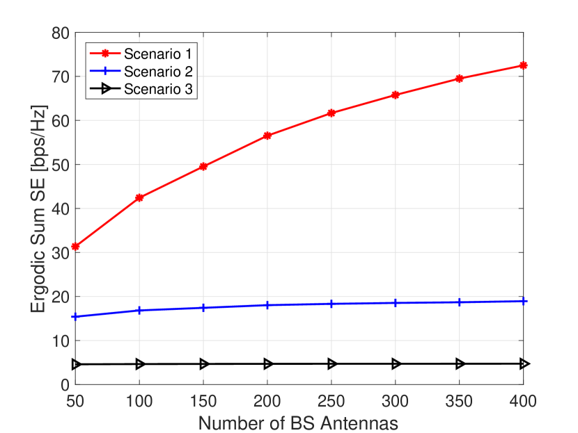
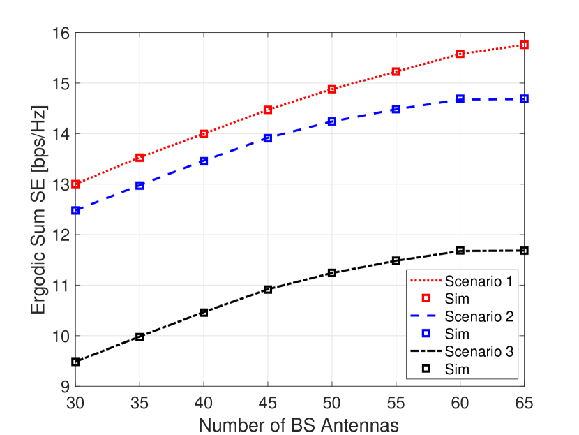
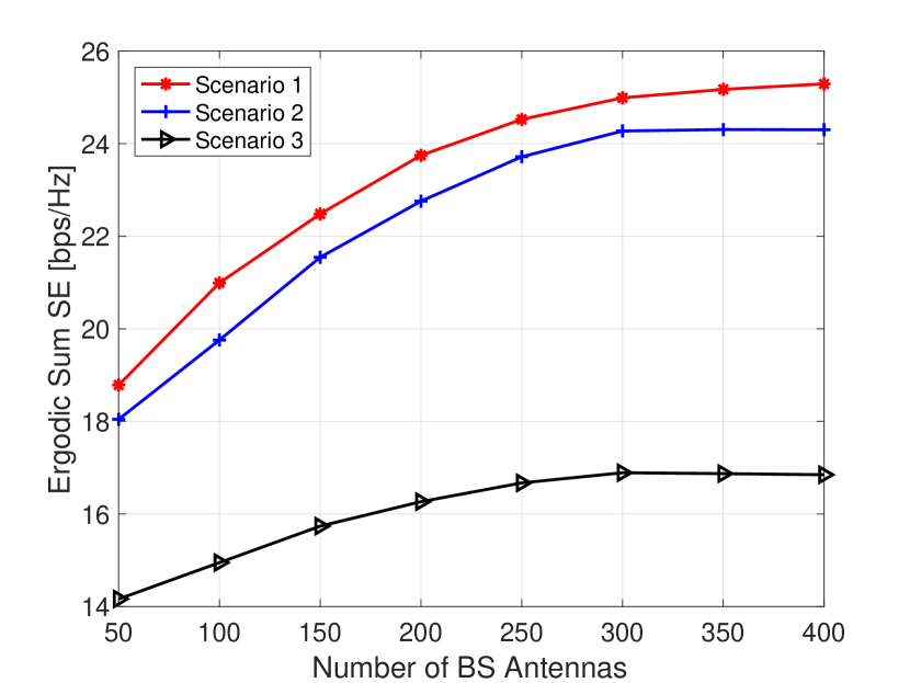
Figure 1: Ergodic UL sum SE for $8$ users and $2$ antennas/user: (a) validation of the closed-form expression, with square markers representing simulation data; (b) SE under jointly correlated Ricean fading; (c) SE under jointly correlated Rayleigh fading.

IV Numerical Results

In this section, we carry out Monte Carlo simulations to validate the closed-form SE expression derived in Section III. We further investigate the system performance under various propagation conditions. All simulation results are obtained for a $20$ MHz channel, a transmit SNR of 10 dB, and a coherence block of $\tau_{c}=500$ symbols. The Ricean factor $\kappa_{k}$ is drawn from $\mathcal{U}(2,4)$ [dB], which is a typical range of values in indoor deployments [17]. The LoS channel component $\bar{\mathbf{H}}_{k}$ is expressed as [18]

$$\bar{\mathbf{H}}_{k}=\sqrt{\frac{\kappa_{k}}{\kappa_{k}+1}}\ \mathbf{a}_{r}\left(\theta^{r}_{k}\right)\cdot\mathbf{a}_{t}\left(\theta^{t}_{k}\right)^{T}$$

where $\theta^{t}_{k}\sim\mathcal{U}(0,2\pi)$ is the angle-of-departure (AoD) of the LoS path, $\theta^{r}_{k}\sim\mathcal{U}(0,2\pi)$ is the angle-of-arrival (AoA), and $\mathbf{a}_{t}\left(\theta^{t}_{k}\right)$ and $\mathbf{a}_{r}\left(\theta^{r}_{k}\right)$ are the transmit and receive array response vectors, respectively. We consider a uniform linear array (ULA) with half-wavelength antenna spacing at both BS and user sides. The array response vectors are then given by

$$\mathbf{a}_{t}\left(\theta^{t}_{k}\right) \triangleq\left[1,e^{j\pi\sin\theta^{t}_{k}},\dots,e^{j\pi(N-1)\sin\theta^{t}_{k}}\right]^{T},$$

$$\mathbf{a}_{r}\left(\theta^{r}_{k}\right) \triangleq\left[1,e^{j\pi\sin\theta^{r}_{k}},\dots,e^{j\pi(M-1)\sin\theta^{r}_{k}}\right]^{T}.$$

IV-A UL Spectral Efficiency

We assess the sum SE of the system under three scenarios:
Scenario 1: $\bm{\Omega}_{k}=\frac{1}{\kappa_{k}+1}\mathbf{1}_{M\times N}$.
Scenario 2: $\bm{\Omega}_{k}=\begin{bmatrix}\frac{MN}{2(\kappa_{k}+1)}&a\mathbf{1}_{1\times(N-1)}\\ a&a\mathbf{1}_{(M-1)\times(N-1)}\end{bmatrix}$, where $a=\frac{MN}{2(\kappa_{k}+1)(MN-1)}$.
Scenario 3: $\bm{\Omega}_{k}=\frac{1}{\kappa_{k}+1}\bm{\lambda}_{k,r}\bm{\lambda}_{k,t}^{T}$, where $\bm{\lambda}_{k,r}$ and $\bm{\lambda}_{k,t}$ are calculated for the coupling matrix of Scenario 2 using the constraints introduced in Section II.
The first scenario represents a rich scattering environment where the NLoS channel components are treated as i.i.d. variables, i.e., uncorrelated Rayleigh fading. The second scenario represents a jointly correlated fading channel where there is an entry in each coupling matrix scaling as $\mathcal{O}(MN)$ [7]. The last scenario is the Kronecker version of the correlated channel considered in Scenario 2. We stress that $\text{tr}(\mathbf{R}_{k})=MN/(\kappa_{k}+1)$ holds in all the scenarios under investigation.

Figure 1(1(a)) shows the accuracy of the closed-form expression against simulation data for 10,000 channel realizations for jointly correlated Ricean fading. As we see, the Kronecker model yields lower SE than the one described by the Weichselberger model, since it neglects the joint correlation feature of the channel, which agrees with the findings in [5]. Next, by capitalizing on the closed-form expression, we plot the sum SE as a function of the number of BS antennas under LoS and NLoS propagation. From Fig. 1(1(b)), we observe that correlation becomes irrelevant in the very large antenna regime due to LoS propagation. Interestingly, due to the presence of LoS components, the SE gains from deploying a massive number of BS antennas are not substantial. Likewise, under NLoS propagation, Fig. 1(1(c)) shows that the SE does not grow without bound as the number of BS antennas increases when at least one entry in the coupling matrix scales as $\mathcal{O}(MN)$. Similar results were reported in [7], [19].

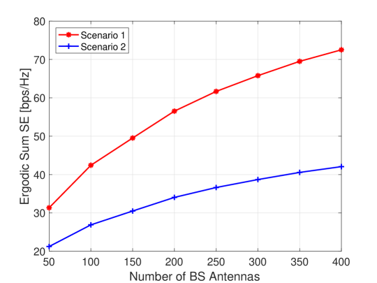
Figure 2: Ergodic UL sum SE for $8$ users and $2$ antennas/user with user precoding and jointly correlated Rayleigh fading.

To circumvent this barrier, we examine the case where users employ precoding. Specifically, we consider that users precode their data with their transmit covariance matrix, i.e., transmit the signal $\sqrt{\rho_{\text{ul}}}\mathbf{U}_{k,t}^{*}\mathbf{s}_{k}$. By doing so, they decorrelate their data streams, and the full correlation matrix takes a block-diagonal form. Figure 2 depicts the sum SE versus the number of BS antennas for NLoS and neglecting the Kronecker-type scenario. We observe that user precoding can enable the sum SE to scale with the number of BS antennas, even when the eigenmode coupling coefficients grow as $\mathcal{O}(MN)$. However, we point out that user precoding entails additional overhead since users have to learn their channel statistics. A similar approach was proposed in [10] for Kronecker-structured systems.

IV-B Multi-Antenna versus Single-Antenna Users

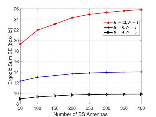
One fundamental question is when additional user antennas are beneficial. In the sequel, we investigate if it is better to serve a few multi-antenna users or many single-antenna users. We assess the sum SE under the correlation Scenario 2 and a total number of data streams $KN=12$. We further consider the options $(12,1),(6,2)$, and $(4,3)$ for the pair $(K,N)$.

Figure 3: Ergodic UL sum SE for different number of served users and user antennas.

From Fig. 3, we notice that having single-antenna users is better in terms of the sum SE compared to the multi-antenna case. We therefore conclude that serving users equipped with multiple antennas is not a good option if sum SE is our objective. However, if we aim at improving other objectives such as per-user SE or communication reliability, using multiple antennas at the users is a meaningful option.

V Conclusions

We analyzed the performance of massive MIMO with multi-antenna users under a generalized channel model. Specifically, we derived a closed-form expression for the UL SE, which is achievable using MR combining and MMSE estimation. Capitalizing on the closed-form expression, we pursued a rigorous study of the system performance. Our SE analysis employs the Weichselberger model, and hence can incorporate the popular Kronecker and virtual channel representation models as special cases. Simulation results suggest that UL SE does not grow always without bound as the number of BS antennas increases under jointly correlated fading, when at least one eigenmode coupling coefficient scales as $\mathcal{O}(MN)$. To circumvent this barrier, we proposed precoding at the users, which entails though additional overhead. In the case of omnidirectional UL transmissions, the detrimental effect of the joint correlation structure of the channel can be alleviated by serving single-antenna users.

Appendix: Proof of Theorem 1

The term $\mathbb{E}[\mathbf{w}_{ki}^{H}\mathbf{h}_{ki}]$ is written as

$$\mathbb{E}[\mathbf{w}_{ki}^{H}\mathbf{h}_{ki}]=\mathbb{E}[\hat{\mathbf{h}}_{ki}^{H}\mathbf{h}_{ki}]=\mathbb{E}[\hat{\mathbf{h}}_{ki}^{H}\hat{\mathbf{h}}_{ki}]+\mathbb{E}[\hat{\mathbf{h}}_{ki}^{H}\hat{\mathbf{e}}_{ki}]$$

$$\overset{(a)}{=}\mathbb{E}[\|\hat{\mathbf{h}}_{ki}\|^{2}]=\text{tr}(\mathbb{E}[\hat{\mathbf{h}}_{ki}\hat{\mathbf{h}}_{ki}^{H}])$$

$$=\text{tr}(\mathbf{\Phi}^{k}_{ii}+\bar{\mathbf{h}}_{ki}\bar{\mathbf{h}}_{ki}^{H})=\text{tr}(\mathbf{\Phi}^{k}_{ii})+\|\bar{\mathbf{h}}_{ki}\|^{2}$$

where $(a)$ is because $\mathbb{E}[\hat{\mathbf{h}}_{ki}^{H}\hat{\mathbf{e}}_{ki}]=0$ under MMSE estimation. We further have $\mathbb{E}[\|\mathbf{w}_{ki}\|^{2}]=\mathbb{E}[\|\hat{\mathbf{h}}_{ki}\|^{2}]=\mathbb{E}[\mathbf{w}_{ki}^{H}\mathbf{h}_{ki}]$, which completes the proof for $\xi_{ki}$.

The second moment $\mathbb{E}[|\mathbf{w}_{ki}^{H}\mathbf{h}_{mj}|^{2}]$ is written as

$$\mathbb{E}[|\mathbf{w}_{ki}^{H}\mathbf{h}_{mj}|^{2}] =\mathbb{E}[|\hat{\mathbf{h}}_{ki}^{H}\mathbf{h}_{mj}|^{2}]$$

$$=\mathbb{E}[|\hat{\mathbf{h}}_{ki}^{H}(\hat{\mathbf{h}}_{mj}+\mathbf{e}_{mj})|^{2}]$$

$$=\mathbb{E}[|\hat{\mathbf{h}}_{ki}^{H}\hat{\mathbf{h}}_{mj}|^{2}]+\mathbb{E}[|\hat{\mathbf{h}}_{ki}^{H}\mathbf{e}_{mj}|^{2}]$$ (15)

where (Appendix: Proof of Theorem 1) follows the fact that the estimation error $\mathbf{e}_{mj}$ has zero mean, and is statistically independent of the channel estimates $\hat{\mathbf{h}}_{ki}$ and $\hat{\mathbf{h}}_{mj}$. Based on this property, we have that

$$\mathbb{E}[|\hat{\mathbf{h}}_{ki}^{H}\mathbf{e}_{mj}|^{2}] =\mathbb{E}\left[\text{tr}\left(\hat{\mathbf{h}}_{ki}^{H}\mathbf{e}_{mj}\mathbf{e}_{mj}^{H}\hat{\mathbf{h}}_{ki}\right)\right]$$

$$=\text{tr}\left(\mathbb{E}\left[\hat{\mathbf{h}}_{ki}\hat{\mathbf{h}}_{ki}^{H}\mathbf{e}_{mj}\mathbf{e}_{mj}^{H}\right]\right)$$

$$=\text{tr}\left(\mathbb{E}\left[\hat{\mathbf{h}}_{ki}\hat{\mathbf{h}}_{ki}^{H}\right]\mathbb{E}\left[\mathbf{e}_{mj}\mathbf{e}_{mj}^{H}\right]\right)$$

$$=\text{tr}(\mathbf{\Phi}^{k}_{ii}\mathbf{C}^{m}_{jj})+\bar{\mathbf{h}}_{ki}^{H}\mathbf{C}^{m}_{jj}\bar{\mathbf{h}}_{ki}.$$ (16)

Combining (Appendix: Proof of Theorem 1) and (Appendix: Proof of Theorem 1) yields

$$\mathbb{E}[|\mathbf{w}_{ki}^{H}\mathbf{h}_{mj}|^{2}]=\mathbb{E}[|\hat{\mathbf{h}}_{ki}^{H}\hat{\mathbf{h}}_{mj}|^{2}]+\text{tr}(\mathbf{\Phi}^{k}_{ii}\mathbf{C}^{m}_{jj})+\bar{\mathbf{h}}_{ki}^{H}\mathbf{C}^{m}_{jj}\bar{\mathbf{h}}_{ki}.$$ (17)

In (17), the term $\mathbb{E}[|\hat{\mathbf{h}}_{ki}^{H}\hat{\mathbf{h}}_{mj}|^{2}]$ is evaluated explicitly for the following three cases:
Case $k\neq m$. The vectors $\hat{\mathbf{h}}_{ki}$ and $\hat{\mathbf{h}}_{mj}$ are statistically independent (i.e., channels of different users). Hence, algebraic manipulations akin to (Appendix: Proof of Theorem 1) yield

$$\begin{multlined}\mathbb{E}[|\hat{\mathbf{h}}_{ki}^{H}\hat{\mathbf{h}}_{mj}|^{2}]=\text{tr}(\mathbf{\Phi}^{k}_{ii}\mathbf{\Phi}^{m}_{jj})+\bar{\mathbf{h}}_{ki}^{H}\mathbf{\Phi}^{m}_{jj}\bar{\mathbf{h}}_{ki}\\ +\bar{\mathbf{h}}_{mj}^{H}\mathbf{\Phi}^{k}_{ii}\bar{\mathbf{h}}_{mj}+|\bar{\mathbf{h}}_{ki}^{H}\bar{\mathbf{h}}_{mj}|^{2}.\end{multlined}\mathbb{E}[|\hat{\mathbf{h}}_{ki}^{H}\hat{\mathbf{h}}_{mj}|^{2}]=\text{tr}(\mathbf{\Phi}^{k}_{ii}\mathbf{\Phi}^{m}_{jj})+\bar{\mathbf{h}}_{ki}^{H}\mathbf{\Phi}^{m}_{jj}\bar{\mathbf{h}}_{ki}\\ +\bar{\mathbf{h}}_{mj}^{H}\mathbf{\Phi}^{k}_{ii}\bar{\mathbf{h}}_{mj}+|\bar{\mathbf{h}}_{ki}^{H}\bar{\mathbf{h}}_{mj}|^{2}.$$ (18)

Combining (17), (18), and the identity $\mathbf{\Phi}^{m}_{jj}=\mathbf{R}^{m}_{jj}-\mathbf{C}^{m}_{jj}$, gives the desired result.
Case $k=m$ and $i=j$. For ease of notation, we drop the subscript $k$. This second moment is computed by writing $\hat{\mathbf{h}}_{i}$ as $\hat{\mathbf{h}}_{i}=\bm{\Phi}_{ii}^{1/2}\mathbf{x}+\bar{\mathbf{h}}_{i}$, where $\mathbf{x}\sim\mathcal{CN}(\mathbf{0},\mathbf{I})$. We then have

$$\mathbb{E} [|\hat{\mathbf{h}}_{i}^{H}\hat{\mathbf{h}}_{i}|^{2}]=\mathbb{E}\left[|(\bm{\Phi}_{ii}^{1/2}\mathbf{x}+\bar{\mathbf{h}}_{i})^{H}(\bm{\Phi}_{ii}^{1/2}\mathbf{x}+\bar{\mathbf{h}}_{i})|^{2}\right]$$

$$=\mathbb{E}\left[|\underbrace{\mathbf{x}^{H}\bm{\Phi}_{ii}\mathbf{x}}_{a}+\underbrace{\mathbf{x}^{H}\bm{\Phi}_{ii}^{1/2}\bar{\mathbf{h}}_{i}}_{b}+\underbrace{\bar{\mathbf{h}}_{i}^{H}\bm{\Phi}_{ii}^{1/2}\mathbf{x}}_{c}+\underbrace{\|\bar{\mathbf{h}}_{i}\|^{2}}_{d}|^{2}\right].$$ (19)

The individual terms are determined as follows. $\mathbb{E}[aa^{*}]=\mathbb{E}[|\mathbf{x}^{H}\mathbf{\Phi}_{ii}\mathbf{x}|^{2}]=|\text{tr}(\mathbf{\Phi}_{ii})|^{2}+\text{tr}(\mathbf{\Phi}_{ii}^{2})$, which is a standard matrix identity [12]; $\mathbb{E}[ab^{*}]=\mathbb{E}[ba^{*}]=0$ because it involves odd order of moments (i.e., multivariate Gaussian distribution); likewise $\mathbb{E}[ac^{*}]=\mathbb{E}[ca^{*}]=0$; $\mathbb{E}[ad^{*}]=\mathbb{E}[da^{*}]=\text{tr}(\mathbf{\Phi}_{ii})\|\bar{\mathbf{h}}_{i}\|$; $\mathbb{E}[bb^{*}]=\bar{\mathbf{h}}_{i}^{H}\mathbf{\Phi}_{ii}\bar{\mathbf{h}}_{i}$; $\mathbb{E}[bc^{*}]=\mathbb{E}[cb^{*}]=0$ due to the circular symmetry of $\mathbf{x}$, i.e., $\mathbb{E}[\mathbf{x}\mathbf{x}^{T}]=0$; $\mathbb{E}[bd^{*}]=\mathbb{E}[db^{*}]=\mathbb{E}[cd^{*}]=\mathbb{E}[dc^{*}]=0$ because $\mathbf{x}$ has zero mean; $\mathbb{E}[cc^{*}]=\bar{\mathbf{h}}_{i}^{H}\mathbf{\Phi}_{ii}\bar{\mathbf{h}}_{i}$; and $\mathbb{E}[dd^{*}]=\|\bar{\mathbf{h}}_{i}\|^{4}$. Thus,

$$\mathbb{E}[|\hat{\mathbf{h}}_{i}^{H}\hat{\mathbf{h}}_{i}|^{2}] =|\text{tr}(\mathbf{\Phi}_{ii})|^{2}+\text{tr}(\mathbf{\Phi}_{ii}^{2})+2\bar{\mathbf{h}}_{i}^{H}\mathbf{\Phi}_{ii}\bar{\mathbf{h}}_{i}$$

$$+2\text{tr}(\mathbf{\Phi}_{ii})\|\bar{\mathbf{h}}_{i}\|+\|\bar{\mathbf{h}}_{i}\|^{4}.$$ (20)

Combining (17) and (Appendix: Proof of Theorem 1) completes the proof.
Case $k=m$ and $i\neq j$. For ease of notation, we drop the subscript $k$ hereafter. In this case, we cannot decompose the vectors $\hat{\mathbf{h}}_{i}$ and $\hat{\mathbf{h}}_{j}$ in terms of a single complex normal Gaussian vector, because the circular symmetry property will not be preserved. According to (5) and (6), we can express $\hat{\mathbf{h}}_{i}$ and $\hat{\mathbf{h}}_{j}$ into the equivalent form $\hat{\mathbf{h}}_{i}=\sum_{l=1}^{N}\tilde{\mathbf{\Phi}}_{il}\mathbf{x}_{l}+\bar{\mathbf{h}}_{i}$ and $\hat{\mathbf{h}}_{j}=\sum_{l=1}^{N}\tilde{\mathbf{\Phi}}_{jl}\mathbf{x}_{l}+\bar{\mathbf{h}}_{j}$, respectively, where $\mathbf{x}_{l}\sim\mathcal{CN}(\mathbf{0},\mathbf{I})$, and $\tilde{\mathbf{\Phi}}_{il}$ denotes the $(i,l$)-th submatrix of $\mathbf{\Phi}^{1/2}$; to see this write $\text{vec}(\hat{\mathbf{H}})=\mathbf{\Phi}^{1/2}[\mathbf{x}_{1}^{T},\dots,\mathbf{x}_{N}^{T}]^{T}+\text{vec}(\bar{\mathbf{H}})$. Also, the following two identities hold

$$\mathbf{\Phi}_{ii} =\sum_{l=1}^{N}\tilde{\mathbf{\Phi}}_{il}\tilde{\mathbf{\Phi}}_{il}^{H}=\sum_{l=1}^{N}\tilde{\mathbf{\Phi}}_{il}\tilde{\mathbf{\Phi}}_{li},$$ (21)

$$\mathbf{\Phi}_{ij} =\sum_{l=1}^{N}\tilde{\mathbf{\Phi}}_{il}\tilde{\mathbf{\Phi}}_{jl}^{H}=\sum_{l=1}^{N}\tilde{\mathbf{\Phi}}_{il}\tilde{\mathbf{\Phi}}_{lj}.$$ (22)

We now have

$$\mathbb{E} [|\hat{\mathbf{h}}_{i}^{H}\hat{\mathbf{h}}_{j}|^{2}]=$$

$$\mathbb{E}\left[\left|\left(\sum_{l_{1}=1}^{N}\tilde{\bm{\Phi}}_{il_{1}}\mathbf{x}_{l_{1}}+\bar{\mathbf{h}}_{i}\right)^{H}\left(\sum_{l_{2}=1}^{N}\tilde{\bm{\Phi}}_{jl_{2}}\mathbf{x}_{l_{2}}+\bar{\mathbf{h}}_{j}\right)\right|^{2}\right].$$

Expanding the product yields an expression akin to (Appendix: Proof of Theorem 1). Utilizing the identities in (21) and (22) and doing some algebra yields several terms similar to the case $i=j$, with the exception of $\mathbb{E}[ad^{*}]=\text{tr}(\mathbf{\Phi}_{ij})\bar{\mathbf{h}}_{i}^{H}\bar{\mathbf{h}}_{j}$, $\mathbb{E}[da^{*}]=(\mathbb{E}[ad^{*}])^{*}$, and $\mathbb{E}[dd^{*}]=|\bar{\mathbf{h}}^{H}_{i}\bar{\mathbf{h}}_{j}|^{2}$. The only term remaining unknown is

$$\mathbb{E}[aa^{*}]=$$

$$\mathbb{E}\left[\left(\sum_{(l_{1},l_{2})}\mathbf{x}_{l_{1}}^{H}\tilde{\bm{\Phi}}_{l_{1}i}\tilde{\bm{\Phi}}_{jl_{2}}\mathbf{x}_{l_{2}}\right)\left(\sum_{(l_{3},l_{4})}\mathbf{x}_{l_{3}}^{H}\tilde{\bm{\Phi}}_{l_{3}i}\tilde{\bm{\Phi}}_{jl_{4}}\mathbf{x}_{l_{4}}\right)^{*}\right].$$

Due to lack of space, we only sketch the proof of that term. If $l_{1}=l_{2}=l_{3}=l_{4}$, we get the standard identity from [12], that is $\sum_{l}\mathbb{E}[|\mathbf{x}_{l}^{H}\tilde{\mathbf{\Phi}}_{li}\tilde{\mathbf{\Phi}}_{jl}\mathbf{x}_{l}|^{2}]=\sum_{l}|\text{tr}(\tilde{\mathbf{\Phi}}_{li}\tilde{\mathbf{\Phi}}_{jl})|^{2}+\|\tilde{\mathbf{\Phi}}_{li}\tilde{\mathbf{\Phi}}_{jl}\|^{2}_{\textsc{f}}$. If at least one of the $l_{i},i=1,\dots,4$, is different from the others, then we have $\mathbb{E}[aa^{*}]=0$ due to the circular symmetry property and the mean value of the individual Guassian vectors. If $l_{1}=l_{2}$ and $l_{3}=l_{4}$, $\mathbb{E}[aa^{*}]=\sum_{l_{1},l_{3}}\text{tr}(\tilde{\mathbf{\Phi}}_{l_{1}i}\tilde{\mathbf{\Phi}}_{jl_{1}})\text{tr}(\tilde{\mathbf{\Phi}}_{il_{3}}\tilde{\mathbf{\Phi}}_{l_{3}j})$. If $l_{1}=l_{3}$ and $l_{2}=l_{4}$, $\mathbb{E}[aa^{*}]=\sum_{l_{1},l_{2}}\|\mathbf{\tilde{\Phi}}_{l_{1}i}\tilde{\mathbf{\Phi}}_{jl_{3}}\|^{2}_{\textsc{f}}$. Finally, if $l_{1}=l_{4}$ and $l_{2}=l_{3}$, $\mathbb{E}[aa^{*}]=0$ due to the circular symmetry property. Putting all the individual terms together completes the proof.

References

• [1] T. L. Marzetta, “Noncooperative cellular wireless with unlimited numbers of base station antennas,” IEEE Trans. Wireless Commun., vol. 9, no. 1, pp. 3590–3600, Nov. 2010.
• [2] H. Q. Ngo, E. G. Larsson, and T. L. Marzetta, “Energy and spectral efficiency of very large multiuser MIMO systems,” IEEE Trans. Commun., vol. 61, no. 4, pp. 1436–1449, Apr. 2013.
• [3] J. P. Kermoal, et al., “A stochastic MIMO radio channel model with experimental validation,” IEEE J. Sel. Areas Commun., vol. 20, no. 6, pp. 1211–1226, Aug. 2002.
• [4] H. Özcelik, M. Herdin, W. Weichselberger, J. Wallace, and E. Bonek, “Deficiencies of the ‘Kronecker’ MIMO radio channel model,” Electron. Lett., vol. 39, no. 16, pp. 1209–1210, Aug. 2003.
• [5] W. Weichselberger, M. Herdin, H. Özcelik, and E. Bonek, “A stochastic MIMO channel model with joint correlation at both link ends,” IEEE Trans. Wireless Commun., vol. 5, no. 1. pp. 90–100, Jan. 2006.
• [6] G. N. Kamga, M. Xia, and S. Aïssa, “Spectral-efficiency analysis of massive MIMO systems in centralized and distributed schemes,” IEEE Trans. Commun. vol. 64, no. 5, pp. 1930–1941, May 2016.
• [7] M. Matthaiou, et al., “Massive MIMO with a generalized channel model: Fundamental aspects,” in Proc. IEEE SPAWC, July 2019.
• [8] Ö. Özdogan, E. Björnson, and E. G. Larsson, “Massive MIMO with spatially correlated Rician fading channels,” IEEE Trans. Commun, vol. 67, no. 5, pp. 3234–3250, May 2019.
• [9] I. Boukhedimi, A. Kammoun, and M. S. Alouini, “Multi-cell MMSE combining over correlated Rician channels in massive MIMO systems,” IEEE Wireless Commun. Let., vol. 9, no. 1, pp. 12–16, Jan. 2020.
• [10] X. Li, E. Björnson, S. Zhou, and J. Wang, “Massive MIMO with multi-antenna users: When are additional user antennas beneficial?” Proc. IEEE ICT, pp. 1–6, May 2016.
• [11] A. M. Sayeed, “Deconstructing multi-antenna fading channels,” IEEE Trans. Signal Process., vol. 50, no. 10, pp. 2563–2579, Oct. 2002.
• [12] E. Björnson, J. Hoydis, and L. Sanguinetti, Massive MIMO Networks: Spectral, Energy, and Hardware Efficiency, Foundations and Trends in Signal Processing: vol. 11, no. 3–4, pp. 154–655, 2017.
• [13] C.-K. Wen, S. Jin, and K.-K. Wong, “On the sum-rate of multiuser MIMO uplink channels with jointly-correlated Rician fading,” IEEE Trans. Commun., vol. 59, no. 10, pp. 2883–2895, Oct. 2011.
• [14] B. Hassibi and B. M. Hochwald, “How much training is needed in multiple-antenna wireless links?,” IEEE Trans. Inf. Theory, vol. 49, no. 4, pp. 951–963, Apr. 2003.
• [15] E. Björnson and B. Ottersten, “A framework for training-based estimation in arbitrarily correlated Rician MIMO channels with Rician disturbance,” IEEE Trans. Signal Process., vol. 58, no. 3, pp. 1807–1820, Mar. 2010.
• [16] T. Yoo and A. Goldsmith, “Capacity and power allocation for fading MIMO channels with channel estimation error,” IEEE Trans. Inf. Theory, vol. 52, no. 5, pp. 2203–2214, May. 2006.
• [17] 3GPP Technical Report 38.802, “Study on new radio access technology; physical layer aspects (Release 14),” Mar. 2017.
• [18] A. G. Burr, “Capacity bounds and estimates for the finite scatterers MIMO wireless channel,” IEEE J. Sel. Areas Commun., vol. 21, no. 5, pp. 812–818, Jun. 2003.
• [19] M. Matthaiou, P. J. Smith, H. Q. Ngo, and H. Tataria, “Does massive MIMO fail in Ricean channels?,” IEEE Wireless Commun. Let., vol. 8, no. 1, pp. 61–64, Feb. 2019.