A fitted finite volume method for stochastic optimal control Problems

Abstract

In this article, we provide a numerical method based on fitted finite volume method to approximate the Hamilton-Jacobi-Bellman (HJB) equation coming from stochastic optimal control problems. The computational challenge is due to the nature of the HJB equation, which may be a second-order degenerated partial differential equation coupled with optimization. In the work, we discretize the HJB equation using the fitted finite volume method and show that matrix resulting from spatial discretization is an M-matrix. The optimization problem is solved at every time step using iterative method. Numerical results are presented to show the robustness of the fitted finite volume numerical method comparing to the standard finite difference method.

1 Introduction

We consider the numerical approximation of the following controlled Stochastic Differential Equation (SDE) defined in $\mathbb{R}^{n}$ ($n\geq 1$) by

$$dx_{t}=b(t,x_{t},\alpha_{t})dt+\sigma(t,x_{t},\alpha_{t})d\omega_{t},\,\,x(0)=x_{0}$$ (1)

where

$$b :[0,T]\times\mathbb{R}^{n}\times\mathcal{A}\rightarrow\mathbb{R}^{n}$$

$$(t,x_{t},\alpha_{t}))\rightarrow b(t,x_{t},\alpha_{t})$$ (2)

is the drift term and

$$\sigma :[0,T]\times\mathbb{R}^{n}\times\mathcal{A}\rightarrow\mathbb{R}^{n\times d}$$

$$(t,x_{t},\alpha_{t}))\rightarrow\sigma(t,x_{t},\alpha_{t})$$ (3)

the d-dimensional diffusion coefficients. Note that $\omega_{t}$ are d-dimensional independent Brownian motion on $\left(\Omega,\mathcal{F},(\mathcal{F}_{t})_{t\geq 0},\mathbb{P}\right)$, $\alpha=(\alpha_{t})_{t\geq 0}$ is an $\mathbb{F}$-adapted process, valued in $\mathcal{A}$ closed convex subset of $\mathbb{R}^{m}\,(m\geq 1)$ and satisfying some integrability conditions and/or state constraints. Precise assumptions on $b$ and $\sigma$ to ensure the existence of the unique solution $x_{t}$ of (1) can be found in [8].
Given a function $g$ from $\mathbb{R}^{n}$ into $\mathbb{R}$ and $f$ from $[0,T]\times\mathbb{R}^{n}\times\mathcal{A}$ into $\mathbb{R}$, the value function is defined by

$$v(t,x)=\underset{\alpha\in\mathcal{A}}{\sup}\,\mathbb{E}\,\left[\int_{t}^{T}f(s,x,\alpha)\,ds+g(x_{T})\right],\,\,\,x\in\mathbb{R}^{n},$$ (4)

and the resulting Hamilton Jacobi-Bellamn (HJB) equation (see [10])is given by

$$\begin{cases}v_{t}(t,x)+\underset{\alpha\in\mathcal{A}}{\sup}\left[L^{\alpha}v(t,x)+f(t,x,\alpha)\right]=0\quad\text{on}\ [0,T)\times\mathbb{R}^{n}\\ v(T,x)=g(x),\,\,\,\,x\,\in\mathbb{R}^{n}\end{cases}$$ (5)

where

$$L^{\alpha}v(t,x)=\sum_{i=1}^{n}(b(t,x,\alpha))_{i}\dfrac{\partial v(t,x)}{\partial x_{i}}+\sum_{i,j=1}^{n}(a(t,x,\alpha))_{i,j}\,\dfrac{\partial^{2}v(t,x)}{\partial x_{i}\,\partial x_{j}},$$ (6)

and $a(t,x,\alpha)=(\dfrac{1}{2}(\sigma(t,x,\alpha))(\sigma(t,x,\alpha))^{T})_{i,j}$.
The existence and uniqueness of the viscosity solution of the HJB equation (5) is well known and can be found in [8]. Equation (5) is a initial value problem. There are two unknown functions in this equation, the value function $v$ and the optimal control $\alpha$. In most practical situations, (5) is not analytically solvable therefore numerical approximations are the only tools appropriate to provide reasonable approximations. Numerical approximation of HJB-equation of type (5) is therefore an active research area and has attracted a lot of attentions [20, 18, 11, 10, 15, 14, 16, 13, 9]. While solving numerically HJB equation, the keys challenge are the low regularity of the solution of HJB equation and the lack of appropriate numerical methods to tackle the degeneracy of the differential operator in HJB equation. Indeed adding to the standard issue that we usually have when solving degenerated PDE, we need to couple with an optimization problem at every grid point and every time step. In terms of existing numerical methods, there are two basic threads of literature concerning controlled HJB equations. A standard approach is based on Markov chain approximation. In financial terms, this approach is equivalent to an explicit finite difference method. However, these methods are well-known to suffer from time step limitations due to stability issues [6]. A more recent approach is based on numerical methods such as finite difference method which ensure convergence to the viscosity solution of the HJB equation couple with an optimization problem at each time [12] .

For many stochastic optimal control problems such as Merton’s control problem, the linear operator is degenerated when the spatial variables approach the region near to zero. This degeneracy has an adverse impact on the accuracy when the finite difference method is used to solve the PDE (see [7], chapter 26). This degeneracy also has an adverse impact on the accuracy of our stochastic optimal control problems since its numerical resolution implies the resolution of PDE, coupled with optimization problem.

In this article, we propose a numerical scheme based on a finite volume method suitable to handle the degeneracy of the linear operator while solving numerically the HJB equation in dimension $1$ and $2$. The method is coupled with implicit time-stepping method for temporal discretization method and the iterative method presented in [9] for optimization problem at every time step. More precisely, this method is based on fitted finite volume technique proposed in [1] to solve the degenerated Black Sholes equations. Note that to the best of our knowledge, such method has not been used to solve the stochastic optimal control problem (5).

The merit of the method is that it is absolutely stable in time because of the implicit nature of the time discretisation and the corresponding matrix after spatial discretization is a positive-definite $M$-matrix.
Numerical simulations prove that our proposed method is more accurate that the standard method based on finite difference spatial discretization.

The rest of this article is organized as follows. In section 2, we present the finite volume method with the fitting technique for dimension 1 and 2. We will also show that the system matrix of the resulting discrete equations is an $M$-matrix. In section 3, we will present the temporal discretization and optimization problem in dimension 1 and 2. Numerical experiments using Matlab software will be performed in section 4 to demonstrate the accuracy of the proposed numerical method. We conclude the work at section 5 by summarizing our finding.

2 Spatial discretization

As we already know, the resolution of the HJB equation (5) involves a spatial discretisation, a temporal discretisation and an optimisation problem at every grid point and each time step. The goal of this section is to provide the spatial discretization of the HJB equation (5) solving our stochastic optimal control problem (4). Details in this section can be found in [4], where such methods have been used to solve the degenerated Black Sholes equation for option pricing with constant coefficients.

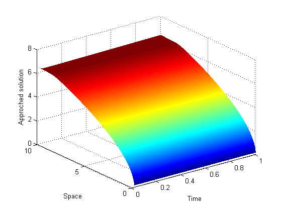
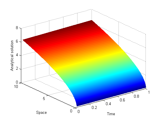
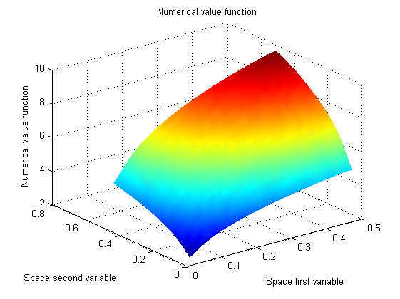
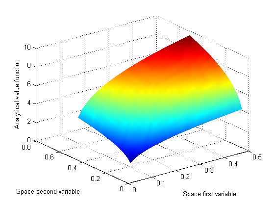
2.1 Spatial discretization based on fitted finite volume method in dimension 1

Consider the more generalized HJB equation (5) in dimension 1 ($n=1$) which can be written in the form.

$$\dfrac{\partial v(x,t)}{\partial t}+\sup_{\alpha\in\mathcal{A}}\left[\dfrac{\partial}{\partial x}\left(a(x,t,\alpha)\,x^{2}\dfrac{\partial v(x,t)}{\partial x}+b(x,t,\alpha)\,x\,v(x,t)\right)+c(x,t,\alpha)\,v(x,t)\right]=0,$$ (7)

where $a(t,x,\alpha)>0$, $\alpha=\alpha(x,t)$ and bounded. As usual, we truncate the problem in the finite interval $I=[0,x_{\text{max}}]$. Let the interval $I=[0,x_{\text{max}}]$ be divided into $N_{1}$ sub-intervals $I_{i}:=(x_{i},x_{i+1}),\,\,\,\,\,i=0\cdots N_{1}-1$ with $0=x_{0}<x_{1}<\cdots\cdots<x_{N_{1}}=x_{\text{max}}$. We also set $x_{i+1/2}=\dfrac{x_{i}+x_{i+1}}{2}$ and $x_{i-1/2}=\dfrac{x_{i-1}+x_{i}}{2}$ for each $i=1\cdots N_{1}-1$ . If we define $x_{-1/2}=x_{0}$ and $x_{N_{1}+1/2}=x_{\text{max}}$ integrating both size of (7) over $J_{i}=\left(x_{i-1/2},\,x_{i+1/2}\right)$ and taking $\alpha_{i}=\alpha(x_{i},t)$, we have

$$\int_{x_{i-1/2}}^{x_{i+1/2}}\dfrac{\partial v}{\partial t}dx+\int_{x_{i-1/2}}^{x_{i+1/2}}\sup_{\alpha_{i}\in\mathcal{A}}\left[\dfrac{\partial}{\partial x}x\left(a(x,t,\alpha_{i})\,x\dfrac{\partial v}{\partial x}+b(x,t,\alpha_{i})\,v\right)+c(x,t,\alpha_{i})\,v\right]dx=0$$ (8)

Applying the mid-points quadrature rule to the first and the last point terms, we obtain the above

$$\dfrac{dv}{dt}l_{i}+\sup_{\alpha_{i}\in\mathcal{A}}\left[\left[x_{i+1/2}\rho(v)\left|{}_{x_{i+1/2}}-x_{i-1/2}\rho(v)\right|_{x_{i-1/2}}\right]+c(x_{i},t,\alpha_{i})\,v_{i}\,l_{i}\right]=0,$$ (9)

for $i=1,2,\cdots N_{1}-1$, where $l_{i}=x_{i+1/2}-x_{i-1/2}$ is the length of $J_{i}$. $v_{i}$ denotes the nodal approximation to $v(\tau,x_{i})$ and $\rho(v)$ is the flux associated with $v$ defined by

$$\rho(v):=a(x,t,\alpha_{i})\,x\,\dfrac{\partial v}{\partial x}+b(x,t,\alpha_{i})\,v.$$ (10)

Clearly, we now need to derive approximation of the flux defined above at the mid-point $x_{i+1/2}$, of the interval $I_{i}$ for $i=2,\cdots N_{1}-1.$ This discussion is divided into two cases for $i\geq 1$ and $I_{0}=(0,x_{1})$.
Case I: Approximation of $\rho$ at $x_{i+1/2}$ for $i\geq 2$.
The term $\left(a(x,t,\alpha_{i})\,x\dfrac{\partial v}{\partial x}+b(x,t,\alpha_{i})\,v\right)$ is approximated by solving the boundary value problem

$$\left(a(x,t,\alpha_{i})\,x\dfrac{\partial v}{\partial x}+b(x_{i+1/2},t,\alpha_{i}),v,\right)^{\prime}=0,\,\,\,\,x\in I_{i}$$ (11)

$$v(x_{i})=v_{i}(t),\,\,v(x_{i+1})=v_{i+1}(t).$$ (12)

Integrating (11) yields the first-order linear equations

$$\rho_{i}(v)(t)=a(x,t,\alpha_{i})\,x\dfrac{\partial v}{\partial x}+b(x_{i+1/2},t,\alpha_{i})\,v=C_{1}$$ (13)

where $C_{1}$ denotes an additive constant. As in [4], the solution is given by

$$v(t)=\dfrac{C_{1}}{b(x_{i+1/2},t,\alpha_{i})}+C_{2}\,x^{-\dfrac{b(x_{i+1/2},t,\alpha_{i})}{a(x_{i+1/2},t,\alpha_{i})}}.$$ (14)

Note that in this deduction we have assumed that $b(x_{i+1/2},t,\alpha_{i})\neq 0$. By setting $\beta_{i}(t)=\dfrac{b(x_{i+1/2},t,\alpha_{i})}{a(x_{i+1/2},t,\alpha_{i})}$, using the boundary conditions in (11) yields

$$v_{i}(t)=\dfrac{C_{1}}{b(x_{i+1/2},t,\alpha_{i})}+C_{2}\,x_{i}^{-\beta_{i}(t)}\,\,\,\text{and}\,\,\,v_{i+1}(t)=\dfrac{C_{1}}{b(x_{i+1/2},t,\alpha_{i})}+C_{2}\,x_{i+1}^{-\beta_{i}(t)}$$ (15)

Solving the following linear system with respect to $C_{1}$ and $C_{2}$ yields

$$\begin{cases}v_{i}(t)=\dfrac{C_{1}}{b(x_{i+1/2},t,\alpha_{i})}+C_{2}\,x_{i}^{-\beta_{i}(t)}\\ v_{i+1}(t)=\dfrac{C_{1}}{b(x_{i+1/2},t,\alpha_{i})}+C_{2}\,x_{i+1}^{-\beta_{i}(t)}\end{cases}$$ (16)

yields

$$\rho_{i}(v)(t)=C_{1}=\dfrac{b(x_{i+1/2},t,\alpha_{i})\,\left(x_{i+1}^{\beta_{i}(t)}v_{i+1}(t)-x_{i}^{\beta_{i}(t)}v_{i}(t)\right)}{x_{i+1}^{\beta_{i}(t)}-x_{i}^{\beta_{i}(t)}}$$ (17)

$\rho_{i}(v)(t)$ provides an approximation to the $\rho(v)(t)$ at $x_{i+1/2}$.
Case II: This is the degenerated zone. The aims here is to approximate $\rho$ at $x_{1/2}$ in the sub-interval $I_{0}$. In this case, the following problem is considered

$$(a(x_{1/2},t,\alpha_{1})\,x\dfrac{\partial v}{\partial x}+b(x_{1/2},t,\alpha_{1})\,v)^{\prime}=C_{2}\,\,\,\textbf{in}\,\,[0,x_{1}]$$ (18)

$$v(0)=v_{0}(t),\,\,\,v(x_{1})=v_{1}(t)$$

where $C_{2}$ is an unknown constant to be determined. Following [4], integrating (18) yields

$$\rho_{0}(v)|_{1/2}(t)=a(x_{1/2},t,\alpha_{i})\,x_{1/2}\dfrac{\partial v}{\partial x}+b(x_{1/2},t,\alpha_{1})\,v=b(x_{1/2},t,\alpha_{1})\,v_{0}(t)+C_{2}\,x_{1/2}.$$ (19)

Since $x_{1/2}=\dfrac{x_{1}+x_{0}}{2}$ with $x_{0}=0$, we have $C_{2}\,x_{1}=(a(x_{1/2},t,\alpha_{1})+b(x_{1/2},t,\alpha_{1}))(v_{1}(t)-v_{0}(t))$. Therefore we have

$$\rho_{0}(v)|_{1/2}(t)=\dfrac{1}{2}\left[(a(x_{1/2},t,\alpha_{1})+b(x_{1/2},t,\alpha_{1}))v_{1}(t)-(a(x_{1/2},t,\alpha_{1})-b(x_{1/2},t,\alpha_{1}))v_{0}(t)\right].$$ (20)

By replacing $\rho$ by its approximated value, (9) becomes for $i=0,1,\cdots,N_{1}-1$

$$\dfrac{dv_{i}(t)}{dt}+\sup_{\alpha_{i}\in\mathcal{A}}\dfrac{1}{l_{i}}\,\left[x_{i+1/2}\dfrac{b(x_{i+1/2},t,\alpha_{i})\,\left(x_{i+1}^{\beta_{i}(t)}v_{i+1}(t)-x_{i}^{\beta_{i}(t)}v_{i}(t)\right)}{x_{i+1}^{\beta_{i}(t)}-x_{i}^{\beta_{i}(t)}}\right.$$ (21)

$$\left.-x_{i-1/2}\dfrac{b(x_{i-1/2},t,\alpha_{i})\,\left(x_{i}^{\beta_{i-1}(t)}v_{i}(t)-x_{i-1}^{\beta_{i-1}(t)}v_{i-1}(t)\right)}{x_{i}^{\beta_{i-1}(t)}-x_{i-1}^{\beta_{i-1}(t)}}+c_{i}(t,\alpha_{i})\,v_{i}(t)\,l_{i}\right]=0$$

By setting $\tau=T-t$ and including the boundary conditions, we have the following system of Ordinary Differential Equation (ODE) coupled with optimisation problem.

$$\begin{cases}-v_{\tau}(\tau)+\underset{\alpha\in\mathcal{A}^{N_{1}-1}}{\sup}\left[A(\alpha,\tau)\,v(\tau)+G(\alpha,\tau)\right]=0\\ v(0)\;\;\text{given},\end{cases}$$ (22)

which can be rewritten as

$$\begin{cases}v_{\tau}(\tau)+\underset{\alpha\in\mathcal{A}^{N_{1}-1}}{\inf}\left[E(\alpha,\tau)\,v(\tau)+F(\alpha,\tau)\right]=0\\ v(0)\;\;\text{given},\end{cases}$$ (23)

where $v(\tau)=(v_{1}(\tau),\cdots,v_{N_{1}-1}(\tau))$ and $F(\alpha,\tau)=(F_{1}(\alpha_{1},\tau),\cdots,F_{N_{1}-1}(\alpha_{N_{1}-1},\tau))$ includes all Dirichlet boundary and final conditions, $A(\alpha,\tau)=-E(\alpha,\tau)$ and $G(\alpha,\tau)=-F(\alpha,\tau)$ are defined as for $i=1,\cdots,N_{1}-1$

$$E_{i,i+1}(\alpha_{i},\tau) =-x_{i+1/2}\dfrac{b_{i+1/2}(\tau,\alpha_{i})\,x_{i+1}^{\beta_{i}(\tau)}}{l_{i}\,(x_{i+1}^{\beta_{i}(\tau)}-x_{i}^{\beta_{i}(\tau)})},$$ (24)

$$E_{i,i}(\alpha_{i},\tau) =\left(x_{i+1/2}\dfrac{b_{i+1/2}(\tau,\alpha_{i})\,x_{i}^{\beta_{i}(\tau)}}{l_{i}\,(x_{i+1}^{\beta_{i}(\tau)}-x_{i}^{\beta_{i}(\tau)})}+x_{i-1/2}\dfrac{b_{i-1/2}(\tau,\alpha_{i})\,x_{i}^{\beta_{i-1}(\tau)}}{l_{i}\,(x_{i}^{\beta_{i-1}(\tau)}-x_{i-1}^{\beta_{i-1}(\tau)})}-c_{i}(\tau,\alpha_{i})\right),$$ (25)

$$E_{i,i-1}(\alpha_{i},\tau) =-x_{i-1/2}\dfrac{b_{i-1/2}(\tau,\alpha_{i})\,x_{i-1}^{\beta_{i-1}(\tau)}}{l_{i}\,(x_{i}^{\beta_{i-1}(\tau)}-x_{i-1}^{\beta_{i-1}(\tau)})},$$ (26)

$$E_{1,1}(\alpha_{1},\tau) =x_{1+1/2}\dfrac{b_{1+1/2}(\tau,\alpha_{1})\,x_{1}^{\beta_{1}(\tau)}}{l_{1}\,(x_{2}^{\beta_{1}(\tau)}-x_{1}^{\beta_{1}(\tau)})}+\dfrac{1}{4\,l_{1}}x_{1}(a_{1/2}(\tau,\alpha_{1})+b_{1/2(\tau,\alpha_{1})})-c_{1}(\tau,\alpha_{1})$$ (27)

$$E_{1,2}(\alpha_{1},\tau) =-x_{1+1/2}\dfrac{b_{1+1/2}(\tau,\alpha_{1})\,x_{2}^{\beta}}{l_{1}\,(x_{2}^{\beta_{1}(\tau)}-x_{1}^{\beta_{1}(\tau)})}$$ (28)

$G(\alpha,\tau)=\left[\begin{array}[]{c}-\dfrac{1}{4\,l_{1}}\,x_{1}(a_{1/2}(\tau,\alpha_{1})-b_{1/2}(\tau,\alpha_{1}))\,v_{0}\\ 0\\ \vdots\\ 0\\ -x_{N_{1}-1/2}\dfrac{b_{N_{1}-1/2}(\tau,\alpha_{N_{1}-1})\,x_{N_{1}}^{\beta_{i}(\tau)}}{l_{N_{1}-1}\,(x_{N_{1}}^{\beta_{N_{1}-1}(\tau)}-x_{N_{1}-1}^{\beta_{N_{1}-1}(\tau)})}v_{N_{1}}\end{array}\right].$

Theorem 2.1

Assume that $c_{i}(\tau,\alpha)<0$, $i=1,\cdots,N_{1}-1$, let $h=\underset{1\leq i\leq N_{1}}{\max}l_{i}$. If $h$ is relatively small then the matrix $E(\alpha,\tau)$ in the system (61) is an M-matrix for any $\alpha\,\in\,\mathcal{A}$.

Proof. Let us show that $E(\alpha,\tau)$ has positive diagonal, non-positive off diagonal, and is diagonally dominant. We first note that

$$\dfrac{b_{i+1/2}(\tau,\alpha)}{x_{i+1}^{\beta_{i}(\tau)}-x_{i}^{\beta_{i}(\tau)}}=\dfrac{a_{i+1/2}(\tau,\alpha)\,\beta_{i}(\tau)}{x_{i+1}^{\beta_{i}(\tau)}-x_{i}^{\beta_{i}(\tau)}}>0,$$ (29)

for $i=1,\cdots,N_{1}-1$, and all $b_{i+1/2}(\tau,\alpha)\neq 0,$ $b_{i-1/2}(\tau,\alpha)\neq 0,$   with $a_{i+1/2}(\tau,\alpha)>0$ and $a_{i-1/2}(\tau,\alpha)>0$.

This also holds when $b_{i+1/2}(\tau,\alpha)\rightarrow 0$ and $b_{i-1/2}(\tau,\alpha)\rightarrow 0$, that is

$$\lim_{b_{i+1/2}(\tau,\alpha)\rightarrow 0}\dfrac{b_{i+1/2}(\tau,\alpha)}{x_{i+1}^{\beta_{i}(\tau)}-x_{i}^{\beta_{i}(\tau)}}=\dfrac{b_{i+1/2}(\tau,\alpha)}{e^{\beta_{i}(\tau)\ln(x_{i+1})}-e^{\beta_{i}(\tau)\ln(x_{i})}}=\dfrac{b_{i+1/2}(\tau,\alpha)}{\beta_{i}(\tau)\ln(x_{i+1})-\beta_{i}(\tau)\ln(x_{i})}$$ (30)

$$=a_{i+1/2}(\tau,\alpha)\left(\ln\dfrac{x_{i+1}}{x_{i}}\right)^{-1}>0,$$

$$\,\lim_{b_{i-1/2}(\tau,\alpha)\rightarrow 0}\dfrac{b_{i-1/2}(\tau)}{x_{i}^{\beta_{i-1}(\tau)}-x_{i-1}^{\beta_{i-1}(\tau)}}=\dfrac{b_{i-1/2}(\tau,\alpha)}{e^{\beta_{i-1}(\tau)\ln(x_{i})}-e^{\beta_{i-1}(\tau)\ln(x_{i-1})}}=\dfrac{b_{i-1/2}(\tau,\alpha)}{\beta_{i-1}(\tau)\ln(x_{i})-\beta_{i-1}(\tau)\ln(x_{i-1})}$$

$$=a_{i-1/2}(\tau,\alpha)\left(\ln\dfrac{x_{i}}{x_{i-1}}\right)^{-1}>0$$

. Using the definition of $E(\alpha,\tau)$ given above, we see that

$$E_{i,i}\geqslant 0,\,\,\,E_{i,i+1}\leqslant 0,\,\,\,E_{i,i-1}\leqslant 0\;\;\;i=2,\cdots,N_{1}-1,$$

$$\left|E_{i,i}\right| \geq\left|E_{i,i-1}\right|+\left|E_{i,i+1}\right|$$

because $x_{i+1}^{\beta_{i}(\tau)}\approx x_{i}^{\beta_{i}(\tau)}+x_{i}^{\beta_{i}(\tau)-1}\,{\beta_{i}(\tau)}\,h$,   $x_{i-1}^{\beta_{i-1}(\tau)}\approx x_{i}^{\beta_{i-1}(\tau)}-x_{i}^{\beta_{i-1}(\tau)-1}\,{\beta_{i-1}(\tau)}\,h$   and

$$\left|E_{i,i}\right|-\left|E_{i,i+1}\right|-\left|E_{i,i-1}\right|$$

$$=-\underset{\rightarrow 0}{\underbrace{\underset{>0}{\underbrace{\left(\dfrac{b_{i+1/2}(\tau)}{x_{i+1}^{\beta_{i}(\tau)}-x_{i}^{\beta_{i}(\tau)}}\right)}}\underset{\rightarrow 0}{\underbrace{\left(h^{\beta_{i}}\,\beta_{i}\,x_{i}^{\beta_{i}-1}\right)}}}}+\underset{\rightarrow 0}{\underbrace{\underset{>0}{\underbrace{\left(\dfrac{b_{i-1/2}(\tau,\alpha)}{x_{i}^{\beta_{i-1}(\tau)}-x_{i-1}^{\beta_{i-1}(\tau)}}\right)}}\underset{\rightarrow 0}{\underbrace{\left(h^{\beta_{i-1}}\,\beta_{i-1}\,x_{i}^{\beta_{i-1}-1}\right)}}}}-c_{i}(\tau,\alpha).$$

Note that for $i=1$, we have $E_{1,1}\geq 0$  if  ${a_{1/2}(\tau,\alpha)}+b_{1/2}(\tau,\alpha)$,  are nonnegative and $c_{1}(\tau,\alpha)<0$. So $E(\alpha,\tau)$ is diagonally dominant and is therefore an M-matrix.  

2.2 Spatial discretization based on fitted finite volume method in dimension 2

Here we consider the following two dimensional problem

$$\dfrac{\partial v(x,y,t)}{\partial t}+\sup_{\alpha\in\mathcal{A}}\left[\nabla\cdot\left(k(x,y,t,\alpha)\right)+c(x,y,t,\alpha)\,v(x,y,t)\right]=0,$$ (31)

where $k(x,y,t,\alpha)=A(x,y,t,\alpha)\cdot\nabla v(x,y,t)+b\,v(x,y,t)$ is the flux,

$b=(x\,b_{1}(x,y,t,\alpha),y\,b_{2}(x,y,t,\alpha))^{T}$ and

$$A=\left(\begin{array}[]{cc}a_{11}&a_{12}\\ a_{21}&a_{22}\end{array}\right),$$

We will assume that $a_{21}=a_{12}$. We also also define the following coefficients, which will help us to build our scheme smoothly $a_{11}(x,y,t,\alpha)=a(x,y,t,\alpha)\,x^{2},a_{22}(x,y,t,\alpha)=\overline{a}(x,y,t,\alpha)y^{2}$ and $a_{12}=a_{21}=d_{1}(x,y,t,\alpha)xy$.

As usual the two dimensional domain is truncated to $I_{x}\times I_{y}$, where $I_{x}=[0,x_{\text{max}}]$ and $I_{y}=[0,y_{\text{max}}]$ be divided into $N_{1}$ and $N_{2}$ sub-intervals:

$$I_{x_{i}}:=(x_{i},x_{i+1}),\,\,I_{y_{j}}:=(y_{j},y_{j+1}),\,\,\,\,i=0,\cdots,N_{1}-1,\,\,j=0,\cdots,N_{2}-1$$

with $0=x_{0}<x_{1}<\cdots\cdots<x_{N_{1}}=x_{\text{max}}$ and $0=y_{0}<y_{1}<\cdots\cdots<y_{N_{2}}=y_{\text{max}}$. This defines a mesh on $I_{x}\times I_{y}$ with all the mesh lines perpendicular to one of the axes.
We also set

$$x_{i+1/2}=\dfrac{x_{i}+x_{i+1}}{2},\,x_{i-1/2}=\dfrac{x_{i-1}+x_{i}}{2},\,y_{j+1/2}=\dfrac{y_{j}+y_{j+1}}{2},\,\;y_{j-1/2}=\dfrac{y_{j-1}+y_{j}}{2},$$

for each $i=1,\cdots,N_{1}-1$ and each $j=1,\cdots,N_{2}-1$. We denote $N=(N_{1}-1)\times(N_{2}-1)$. These mid-points form a second partition of $I_{x}\times I_{y}$ if we define $x_{-1/2}=x_{0}$, $x_{N_{1}+1/2}=x_{\text{max}}$,  $y_{-1/2}=y_{0}$ and $y_{N_{2}+1/2}=y_{\text{max}}$. For each $i=0,1,\cdots,N_{1}$ and $j=0,1,\cdots,N_{2}$, we set $h_{x_{i}}=x_{i+1/2}-x_{i-1/2}$ and $h_{y_{j}}=y_{j+1/2}-y_{j-1/2}$.
We now discuss the finite volume method for (31). Integrating both size of (31) over $\mathcal{R}_{i,j}=\left[x_{i-1/2},x_{i+1/2}\right]\times\left[y_{j-1/2},y_{j+1/2}\right]$, we have

$$\int_{x_{i-1/2}}^{x_{i+1/2}}\int_{y_{j-1/2}}^{y_{j+1/2}}\dfrac{\partial v}{\partial t}\,dx\,dy+\int_{x_{i-1/2}}^{x_{i+1/2}}\int_{y_{j-1/2}}^{y_{j+1/2}}\sup_{\alpha\in\mathcal{A}}\left[\nabla\cdot\left(k(v(x,y,t,\alpha))\right)+c(x,y,t,\alpha)\,v(x,y,t)\right]\,dx\,dy=0,$$ (32)

for $i=1,2,\cdots,N_{1}-1$,  $j=1,2,\cdots,N_{2}-1$. Applying the mid-points quadrature rule to the first and the last point terms, we obtain the above

$$\dfrac{dv_{i,j}(t)}{dt}\,l_{i,j}+\sup_{\alpha_{i,j}\in\mathcal{A}}\left[\int_{\partial\mathcal{R}_{i,j}}\nabla\cdot\left(k(v(x,y,t,\alpha_{i,j})\right)\,dx\,dy+c_{i,j}(t,\alpha_{i,j})\,v_{i,j}(t)\,l_{i,j}\right]=0$$ (33)

for $i=1,2,\cdots N_{1}-1$,  $j=1,2,\cdots N_{2}-1$ where $l_{i,j}=\left(x_{i+1/2}-x_{i-1/2}\right)\times\left(y_{j+1/2}-y_{j-1/2}\right)$ is the length of $\mathcal{R}_{i,j}$, and $v_{i,j}(t)$ denotes the nodal approximation to $v(x_{i},y_{j},t)$. We now consider the approximation of the middle term in (33). Let $\bf n$ denote the unit vector outward-normal to $\partial\mathcal{R}_{i,j}$. By Ostrogradski Theorem, integrating by parts and using the definition of flux $k$, we have

$$\int_{\mathcal{R}_{i,j}}\nabla\cdot\left(k(v)\right) =\int_{\partial\mathcal{R}_{i,j}}k(v(x,y,t,\alpha_{i,j}))\cdot\bf n\,ds$$

$$=\int_{\left(x_{i+1/2},y_{j-1/2}\right)}^{\left(x_{i+1/2},y_{j+1/2}\right)}\left(a_{11}\,\dfrac{\partial v}{\partial x}+a_{12}\,\dfrac{\partial v}{\partial y}+x\,b_{1}\,v\right)dy$$ (34)

$$-\int_{\left(x_{i-1/2},y_{j-1/2}\right)}^{\left(x_{i-1/2},y_{j+1/2}\right)}\left(a_{11}\,\dfrac{\partial v}{\partial x}+a_{12}\,\dfrac{\partial v}{\partial y}+xb_{1}\,v\right)dy$$

$$+\int_{\left(x_{i-1/2},y_{j+1/2}\right)}^{\left(x_{i+1/2},y_{j+1/2}\right)}\left(a_{21}\,\dfrac{\partial v}{\partial x}+a_{22}\,\dfrac{\partial v}{\partial y}+y\,b_{2}\,v\right)dx$$

$$-\int_{\left(x_{i-1/2},y_{j-1/2}\right)}^{\left(x_{i+1/2},y_{j-1/2}\right)}\left(a_{21}\,\dfrac{\partial v}{\partial x}+a_{22}\,\dfrac{\partial v}{\partial y}+y\,b_{2}\,v\right)dx.$$

We shall look at (2.2) term by term. For the first term we want to approximate the integral by a constant as

$$\int_{\left(x_{i+1/2},y_{j-1/2}\right)}^{\left(x_{i+1/2},y_{j+1/2}\right)}\left(a_{11}\,\dfrac{\partial v}{\partial x}+a_{12}\,\dfrac{\partial v}{\partial y}+x\,b_{1}\,v\right)dy$$ (35)

$$\approx\left(a_{11}\,\dfrac{\partial v}{\partial x}+a_{12}\,\dfrac{\partial v}{\partial y}+x\,b_{1}\,v\right)|_{\left(x_{i+1/2},y_{j}\right)}\cdot h_{y_{j}}.$$

To achieve this, it is clear that we now need to derive approximations of the $k(v(x,y,t,\alpha_{i,j}))\cdot\bf n$ defined above at the mid-point $\left(x_{i+1/2},y_{j}\right)$, of the interval $I_{x_{i}}$ for $i=0,1,\cdots N_{1}-1$. This discussion is divided into two cases for $i\geq 1$ and $i\,\in I_{0}=(0,x_{1})$. This is really an extension of the one dimensional fitted finite volume presented in the previous section.

Case I: For $i\geq 2$.

Remember that $a_{11}(x,y,t,\alpha)=a(x,y,t,\alpha)\,x^{2}$, we approximate the term $\left(a_{11}\dfrac{\partial v}{\partial x}+x\,b_{1}\,v\right)$ by solving the following two points boundary value problem

$$\left({a}(x_{i+1/2},y_{j},t,\alpha_{i,j})\,x_{i+1/2}\dfrac{\partial v}{\partial x}+b_{1}(x_{i+1/2},y_{j},t,\alpha_{i,j})\,v\right)^{\prime}=0$$ (36)

$$\hskip 71.13188ptv(x_{i},y_{j},t)=v_{i,j}(t),\,\,\,\,v(x_{i+1},y_{j},t)=v_{i+1,j}(t).$$

Integrating (36) yields the first-order linear equations

$${a}(x_{i+1/2},y_{j},t,\alpha_{i,j})\,x_{i+1/2}\dfrac{\partial v}{\partial x}+b_{1}(x_{i+1/2},y_{j},t,\alpha_{i,j})\,v=C_{1}$$ (37)

where $C_{1}$ denotes an additive constant. Following the one dimensional fitted finite volume presented in the previous section, we have

$$C_{1}=\dfrac{{b_{1}}_{i+1/2,j}(t,\alpha_{i,j})\,\left(x_{i+1}^{\beta_{i,j}(t)}\,v_{i+1,j}-x_{i}^{\beta_{i,j}(t)}v_{i,j}\right)}{x_{i+1}^{\beta_{i,j}(t)}-x_{i}^{\beta_{i,j}(t)}}.$$ (38)

Therefore,

$$a_{11}\,\dfrac{\partial v}{\partial x}+a_{12}\,\dfrac{\partial v}{\partial y}+x\,b_{1}\,v\approx x_{i+1/2}\left(\dfrac{{b_{1}}_{i+1/2,j}(t,\alpha_{i,j})\,\left(x_{i+1}^{\beta_{i,j}(t)}v_{i+1,j}-x_{i}^{\beta_{i,j}(t)}\,v_{i,j}\right)}{x_{i+1}^{\beta_{i,j}(t)}-x_{i}^{\beta_{i,j}(t)}}+d_{1}\,y\,\,\dfrac{\partial v}{\partial y}\right),$$ (39)

where $\beta_{i,j}(t)=\dfrac{{b_{1}}_{i+1/2,j}(t,\alpha_{i,j})}{{a}_{i+1/2,j}(t,\alpha_{i,j})}$ and $a_{12}=a_{21}=d_{1}(x,y,t,\alpha)\,x\,y$. Finally, we use the forward difference,

$$\dfrac{\partial v}{\partial y}\approx\dfrac{v_{i,j+1}-v_{i,j}}{h_{y_{j}}}$$

Finally,

$$\left[a_{11}\,\dfrac{\partial v}{\partial x}+a_{12}\,\dfrac{\partial v}{\partial y}+x\,b_{1}\,v\right]_{\left(x_{i+1/2},y_{j}\right)}\cdot h_{y_{j}}$$

$$\approx x_{i+1/2}\left(\dfrac{{b_{1}}_{i+1/2,j}(t,\alpha_{i,j})\,\left(x_{i+1}^{\beta_{i,j}(t)}v_{i+1,j}-x_{i}^{\beta_{i,j}(t)}\,v_{i,j}\right)}{x_{i+1}^{\beta_{i,j}(t)}-x_{i}^{\beta_{i,j}(t)}}+{d_{1}}_{i,j}(t,\alpha_{i,j})\,y_{j}\,\dfrac{v_{i,j+1}-v_{i,j}}{h_{y_{j}}}\right)\cdot h_{y_{j}}.$$ (40)

Simillary, the second term in (2.2) can be approximated by

$$\left[a_{11}\,\dfrac{\partial v}{\partial x}+a_{12}\,\dfrac{\partial v}{\partial y}+x\,b_{1}\,v\right]_{\left(x_{i-1/2},{y_{j}}\right)}\cdot h_{y_{j}}$$

$$\approx x_{i-1/2}\left(\dfrac{{b_{1}}_{i-1/2,j}(t,\alpha_{i,j})\,\left(x_{i}^{\beta_{i-1,j}(t)}v_{i,j}-x_{i-1}^{\beta_{i-1,j}(t)}v_{i-1,j}\right)}{x_{i}^{\beta_{i-1,j}(t)}-x_{i-1}^{\beta_{i-1,j}(t)}}+{d_{1}}_{i,j}(t,\alpha_{i,j})\,y_{j}\,\dfrac{v_{i,j+1}-v_{i,j}}{h_{{y_{j}}}}\right)\cdot h_{y_{j}}.$$ (41)

Case II: For $j\geq 2$.

For the third term we want to approximate the integral by a constant, that is

$$\int_{\left(x_{i-1/2},y_{j+1/2}\right)}^{\left(x_{i+1/2},y_{j+1/2}\right)}\left(a_{21}\,\dfrac{\partial v}{\partial x}+a_{22}\,\dfrac{\partial v}{\partial y}+y\,b_{2}\,v\right)dx$$ (42)

$$\approx\left(a_{21}\,\dfrac{\partial v}{\partial x}+a_{22}\,\dfrac{\partial v}{\partial y}+y\,b_{2}\,v\right)|_{\left({y_{j+1/2}},x_{i}\right)}\cdot h_{x_{i}}.$$

Following the first case of this section, we have

$$\left[a_{21}\,\dfrac{\partial v}{\partial x}+a_{22}\,\dfrac{\partial v}{\partial x_{2}}+y\,b_{2}\,v\right]_{\left(x_{i},{y_{j+1/2}}\right)}\cdot h_{x_{i}}$$

$$\approx y_{j+1/2}\left(\dfrac{{b_{2}}_{i,j+1/2}(t,\alpha_{i,j})\,\left({y_{j+1}}^{\bar{\beta}_{i,j}(t)}v_{i,j+1}-{y_{j}}^{\bar{\beta}_{i,j}(t)}\,v_{i,j}\right)}{{y_{j+1}}^{\bar{\beta}_{i,j}(t)}-{y_{j}}^{\bar{\beta}_{i,j}(t)}}+{d_{1}}_{i,j}(t,\alpha_{i,j})\,x_{i}\,\dfrac{v_{i+1,j}-v_{i,j}}{h_{x_{i}}}\right)\cdot h_{x_{i}}.$$ (43)

Similary, the fourth term in (2.2) can be approximated by

$$\left[a_{21}\,\dfrac{\partial v}{\partial x}+a_{22}\,\dfrac{\partial v}{\partial y}+y\,b_{2}\,v\right]_{\left(x_{i},y_{j-1/2}\right)}\cdot h_{x_{i}}\approx$$

$$y_{j-1/2}\left(\dfrac{{b_{2}}_{i,j-1/2}(t,\alpha_{i,j})\,\left(y_{j}^{\bar{\beta}_{i,j-1}(t)}\,v_{i,j}-y_{j-1}^{\bar{\beta}_{i,j-1}(t)}\,v_{i,j-1}\right)}{y_{j}^{\bar{\beta}_{i,j-1}(t)}-y_{j-1}^{\bar{\beta}_{i,j-1}(t)}}+{d_{1}}_{i,j}(t,\alpha_{i,j})\,x_{i}\,\dfrac{v_{i+1,j}-v_{i,j}}{h_{x_{i}}}\right)\cdot h_{x_{i}},$$ (44)

for $j=2,\cdots,N_{2}-1$, where $\bar{\beta}_{i,j}(t)=\dfrac{{b_{2}}_{i,j+1/2}(t,\alpha_{i,j})}{\bar{a}_{i,j+1/2}(t,\alpha_{i,j})}$ with $a_{22}(x,y,t,\alpha)=\bar{a}(x,y,t,\alpha)\,y^{2}$.

Case III: Approximation of the flux at $I_{0}$. Note that the analysis in case I does not apply to the approximation of the flux on $[0,x_{1}]$ because (36) is degenerated. Therefore, we reconsider the following form

$$(a(x_{1/2},y_{j},t,\alpha_{1,j})\,x_{1/2}\dfrac{\partial v}{\partial x}+{b_{1}}(x_{1/2},y,t,\alpha_{1,j})\,v)^{\prime}\equiv C_{2}\,\,\,\textbf{in}\,\,[0,x_{1}]$$ (45)

$$v(x_{0},y_{j})=v_{0,j},\,\,\,\,v(x_{1},{y_{j}})=v_{1,j},$$

where $C_{2}$ is an unknown constant to be determined. Integrating (45), we can deduce that

$$\left[a_{11}\,\dfrac{\partial v}{\partial x}+a_{12}\,\dfrac{\partial v}{\partial y}+x\,b_{1}\,v\right]_{\left(x_{1/2},{y_{j}}\right)}\cdot h_{y_{j}}$$

$$\approx x_{1/2}\left(\dfrac{1}{2}\left[(a_{x_{1/2},j}(t,\alpha_{1,j})+{b_{1}}_{x_{1/2},j}(t,\alpha))\,v_{1,j}-(a_{x_{1/2},j}(t,\alpha_{1,j})-{b_{1}}_{x_{1/2},j}(t,\alpha_{1,j}))\,v_{0,j}\right]\right.$$ (46)

$$\left.+{d_{1}}_{1,j}(t,\alpha_{1,j})\,y_{j}\,\dfrac{v_{1,j+1}-v_{1,j}}{h_{y_{j}}}\right)\cdot h_{y_{j}}.$$

Case IV: Approximation of the flux at $J_{0}$.

Using the same procedure for the approximation of the flux at $I_{0}$, we deduce that

$$\left[a_{21}\,\dfrac{\partial v}{\partial x}+a_{22}\,\dfrac{\partial v}{\partial y}+y\,b_{2}\,v\right]_{\left(x_{i},{y_{1/2}}\right)}\cdot h_{x_{i}}\approx$$

$$y_{1/2}\left(\dfrac{1}{2}\left[(\bar{a}_{i,y_{1/2}}(t,\alpha_{i,1})+{b_{2}}_{i,y_{1/2}}(t,\alpha))\,v_{i,1}-(\bar{a}_{i,y_{1/2}}(t,\alpha_{i,1})-{b_{2}}_{i,y_{1/2}}(t,\alpha_{i,1}))\,v_{i,0}\right]\right.$$ (47)

$$\left.+{d_{1}}_{i,1}(t,\alpha_{i,1})\,x_{i}\,\dfrac{v_{i+1,1}-v_{i,1}}{h_{x_{i}}}\right)\cdot h_{x_{i}}.$$

By replacing the flux by his value for $i=1,\cdots,N_{1}-1$ and $j=1,\cdots,N_{2}-1$, equation (33) becomes

$$\dfrac{dv_{i,j}}{dt}$$ (48)

$$+\sup_{\alpha_{i,j}\in\mathcal{A}}\dfrac{1}{l_{i,j}}\,\left[x_{{i+1/2}}\left(\dfrac{{b_{1}}_{i+1/2,j}(t,\alpha)\,\left(x_{{i+1}}^{\beta_{i,j}(t)}\,v_{i+1,j}-x_{{i}}^{\beta_{i,j}(t)}\,v_{i,j}\right)}{x_{{i+1}}^{\beta_{i,j}(t)}-x_{{i}}^{\beta_{i,j}(t)}}+{d_{1}}_{i,j}(t,\alpha_{i,j})\,y_{j}\,\dfrac{v_{i,j+1}-v_{i,j}}{h_{y_{j}}}\right)\cdot h_{y_{j}}\right.$$

$$\left.-x_{{i-1/2}}\left(\dfrac{{b_{1}}_{i-1/2,j}(t,\alpha_{i,j})\,\left(x_{i}^{\beta_{i-1,j}}\,v_{i,j}-x_{{i-1}}^{\beta_{i-1,j}(t)}\,v_{i-1,j}\right)}{x_{{i}}^{\beta_{i-1,j}(t)}-x_{{i-1}}^{\beta_{i-1,j}(t)}}+{d_{1}}_{i,j}(t,\alpha_{i,j})\,y_{j}\,\dfrac{v_{i,j+1}-v_{i,j}}{h_{{y_{j}}}}\right)\cdot h_{{y_{j}}}\right.$$

$$\left.+{y_{j+1/2}}\left(\dfrac{{b_{2}}_{i,j+1/2}(t,\alpha_{i,j})\,\left({y_{j+1}}^{\bar{\beta}_{i,j}(t)}\,v_{i,j+1}-{y_{j}}^{\bar{\beta}_{i,j}(t)}v_{i,j}\right)}{{y_{j+1}}^{\bar{\beta}_{i,j}(t)}-{y_{j}}^{\bar{\beta}_{i,j}(t)}}+{d_{1}}_{i,j}(t,\alpha_{i,j})\,x_{i}\,\dfrac{v_{i+1,j}-v_{i,j}}{h_{x_{i}}}\right)\cdot h_{x_{i}}\right.$$

$$\left.-{y_{j-1/2}}\left(\dfrac{{b_{2}}_{i,j-1/2}(t,\alpha_{i,j})\,\left({y_{j}}^{\bar{\beta}_{i,j-1}(t)}v_{i,j}-{y_{j-1}}^{\bar{\beta}_{i,j-1}(t)}\,v_{i,j-1}\right)}{{y_{j}}^{\bar{\beta}_{i,j-1}(t)}-{y_{j-1}}^{\bar{\beta}_{i,j-1}(t)}}\right.\right.$$

$$\left.\left.+{d_{1}}_{i,j}(t,\alpha_{i,j})\,x_{i}\,\dfrac{v_{i+1,j}-v_{i,j}}{h_{x_{i}}}\right)\cdot h_{x_{i}}+c_{i,j}(t,\alpha_{i,j})\,v_{i,j}\,l_{i,j}\right]=0$$

By setting $\tau=T-t$ and including the boundary conditions, we have the following system

$$\begin{cases}&\underset{\alpha\in\mathcal{A}^{N}}{\sup}\,\left[e_{i-1,j}^{i,j}(\tau,\alpha)\,v_{i-1,j}+e_{i,j}^{i,j}(\tau,\alpha)\,v_{i,j}+e_{i+1,j}^{i,j}(\tau,\alpha)\,v_{i+1,j}+e_{i,j-1}^{i,j}(\tau,\alpha)v_{i,j-1}+e_{i,j+1}^{i,j}(\tau,\alpha)v_{i,j+1}\right]\\ &-\dfrac{dv_{i,j}}{d\tau}=0,\,\,\mbox{with}~{}~{}\,\,\,\,v(0)\,\,\,\text{given},\end{cases}$$ (49)

where for $i=1,\cdots,N_{1}-1$, $j=1,\cdots,N_{2}-1$ and $N=(N_{1}-1)\times(N_{2}-1)$, we have

$$e_{0,j}^{1,j} =-\dfrac{1}{4\,l_{1,j}}h_{{y_{j}}}\,x_{1}(a_{x_{1/2},j}(\tau,\alpha_{1,j})-{b_{1}}_{x_{1/2},j}(\tau,\alpha_{1,j}))\,v_{0,j}$$ (50)

$$e_{1,j}^{1,j} =\dfrac{1}{4\,l_{1,j}}h_{{y_{j}}}\,x_{1}(a_{x_{1/2},j}(\tau,\alpha_{1,j})+{b_{1}}_{x_{1/2},j}(\tau,\alpha_{1,j}))-\dfrac{1}{2}\,c_{1,j}(\tau,\alpha_{1,j})+{d_{1}}_{1,j}(\tau,\alpha_{1,j})\,x_{i}\dfrac{h_{{y_{j}}}}{l_{1,j}}$$

$$+x_{{1+1/2}}h_{{y_{j}}}\dfrac{{b_{1}}_{1+1/2,j}(\tau,\alpha_{1,j})\,x_{{1}}^{\beta_{1,j}(\tau)}}{l_{1,j}\left(x_{{2}}^{\beta_{1,j}(\tau)}-x_{{1}}^{\beta_{1,j}(\tau)}\right)}$$ (51)

$$e_{2,j}^{1,j} =-{d_{1}}_{1,j}(\tau,\alpha_{1,j})\,x_{i}\,\dfrac{h_{{y_{j}}}}{l_{1,j}}-x_{{1+1/2}}h_{{y_{j}}}\dfrac{{b_{1}}_{1+1/2,j}(\tau,\alpha_{1,j})\,x_{{2}}^{\beta_{1,j}(\tau)}}{l_{1,j}\left(x_{{2}}^{\beta_{1,j}(\tau)}-x_{{1}}^{\beta_{1,j}(\tau)}\right)}$$ (52)

$$e_{i,0}^{i,1} =-\dfrac{1}{4\,l_{i,1}}h_{x_{i}}\,y_{1}(\bar{a}_{i,y_{1/2}}(\tau,\alpha_{i,1})-{b_{2}}_{i,y_{1/2}}(\tau,\alpha_{i,1}))\,v_{i,0}$$ (53)

$$e_{i,1}^{i,1} =\dfrac{1}{4\,l_{i,1}}h_{x_{i}}\,y_{1}(\bar{a}_{i,y_{1/2}}(\tau,\alpha_{i,1})+{b_{2}}_{i,y_{1/2}}(\tau,\alpha_{i,1})-\dfrac{1}{2}\,c_{i,1}(\tau,\alpha_{i,1})+{d_{1}}_{i,1}(\tau,\alpha_{i,1})\,y_{j}\,\dfrac{h_{x_{i}}}{l_{i,1}}$$

$$+y_{{1+1/2}}h_{x_{i}}\dfrac{{b_{2}}_{i,1+1/2}(\tau,\alpha_{i,1})\,y_{{1}}^{\bar{\beta}_{i,1}(\tau)}}{l_{i,1}\left(y_{{2}}^{\bar{\beta}_{i,1}(\tau)}-y_{{1}}^{\bar{\beta}_{i,1}(\tau)}\right)}$$ (54)

$$e_{i,2}^{i,1} =-{d_{1}}_{i,1}(\tau,\alpha_{i,1})\,y_{j}\,\dfrac{h_{x_{i}}}{l_{i,1}}-{y_{1+1/2}}h_{x_{i}}\dfrac{{b_{2}}_{i,1+1/2}(\tau,\alpha_{i,1})\,{y_{2}}^{\bar{\beta}_{i,1}(\tau)}}{l_{i,1}\left({y_{2}}^{\bar{\beta}_{i,1}(\tau)}-{y_{1}}^{\bar{\beta}_{i,1}(\tau)}\right)}$$ (55)

$$e_{i+1,j}^{i,j} =-{d_{1}}_{i,j}(\tau,\alpha_{i,j}))\,\dfrac{h_{{y_{j}}}}{l_{i,j}}-x_{{i+1/2}}h_{{y_{j}}}\dfrac{{b_{1}}_{i+1/2}(\tau,\alpha_{i,j})\,x_{{i+1}}^{\beta_{i,j}(\tau)}}{l_{i,j}\left(x_{{i+1}}^{\beta_{i,j}(\tau)}-x_{{i}}^{\beta_{i,j}(\tau)}\right)}$$ (56)

$$e_{i-1,j}^{i,j} =-x_{{i-1/2}}h_{{y_{j}}}\dfrac{{b_{1}}_{{i-1/2,j}}(\tau,\alpha_{i,j}))\,x_{{i-1}}^{\beta_{i-1,j}(\tau)}}{l_{i,j}\left(x_{{i}}^{\beta_{i-1,j}(\tau)}-x_{{i-1}}^{\beta_{i-1,j}(\tau)}\right)}$$ (57)

$$e_{i,j}^{i,j} ={d_{1}}_{i,j}(\tau,\alpha_{i,j}))\,x_{i}\,\dfrac{h_{{y_{j}}}}{l_{i,j}}+x_{{i+1/2}}h_{{y_{j}}}\dfrac{{b_{1}}_{{i+1/2,j}}(\tau,\alpha_{i,j}))\,x_{{i}}^{\beta_{i,j}(\tau)}}{l_{i,j}\left(x_{{i+1}}^{\beta_{i,j}(\tau)}-x_{{i}}^{\beta_{i,j}(\tau)}\right)}$$ (58)

$$+x_{{i-1/2}}h_{{y_{j}}}\dfrac{{b_{1}}_{{i-1/2,j}}(\tau,\alpha_{i,j}))\,x_{{i}}^{\beta_{i-1,j}(\tau)}}{l_{i,j}\left(x_{{i}}^{\beta_{i-1,j}(\tau)}-x_{{i-1}}^{\beta_{i-1,j}(\tau)}\right)}-c_{i,j}(\tau,\alpha_{i,j}))$$

$${d_{1}}_{i,j}(\tau,\alpha_{i,j}))\,y_{j}\,\dfrac{h_{x_{i}}}{l_{i,j}}+{y_{j+1/2}}h_{x_{i}}\dfrac{{b_{2}}_{i,j+1/2}(\tau,\alpha_{i,j}))\,{y_{j}}^{\bar{\beta}_{i,j}(\tau)}}{l_{i,j}\left({y_{j+1}}^{\bar{\beta}_{i,j}(\tau)}-{y_{j}}^{\bar{\beta}_{i,j}(\tau)}\right)}$$

$$+{y_{j-1/2}}h_{x_{i}}\dfrac{{b_{2}}_{i,j-1/2}(\tau,\alpha_{i,j}))\,{y_{j}}^{{\beta}_{i,j-1}(\tau)}}{l_{i,j}\left({y_{j}}^{\bar{\beta}_{i,j-1}(\tau)}-{y_{j-1}}^{\bar{\beta}_{i,j-1}(\tau)}\right)}$$

$$e_{i,j+1}^{i,j} =-{d_{1}}_{i,j}(\tau,\alpha_{i,j}))\,y_{j}\,\dfrac{h_{x_{i}}}{l_{i,j}}-y_{{j+1/2}}h_{x_{i}}\dfrac{{b_{2}}_{{i,j+1/2}}(\tau,\alpha_{i,j}))\,{y_{j+1}}^{\bar{\beta}_{i,j}(\tau)}}{l_{i,j}\left({y_{j+1}}^{\bar{\beta}_{i,j}(\tau)}-{y_{j}}^{\bar{\beta}_{i,j}(\tau)}\right)}$$ (59)

$$e_{i,j-1}^{i,j} =-{y_{j-1/2}}h_{x_{i}}\dfrac{{b_{2}}_{i,j-1/2}(\tau,\alpha_{i,j}))\,{y_{j-1}}^{\bar{\beta}_{i,j-1}(\tau)}}{l_{i,j}\left({y_{j}}^{\bar{\beta}_{i,j-1}(\tau)}-{y_{j-1}}^{\bar{\beta}_{i,j-1}(\tau)}\right)}.$$ (60)

As for one dimension case, (49) can be rewritten as the Ordinary Differential Equation (ODE) coupled with optimization problem

$$\begin{cases}\dfrac{d\textbf{v}(\tau)}{d\tau}+\underset{\alpha\in\mathcal{A}^{N}}{\inf}\,\left[E(\tau,\alpha)\,\textbf{v}(\tau)+F(\tau,,\alpha)\right]=0,\\ ~{}~{}~{}\mbox{with}~{}~{}\,\,\,\,\textbf{v}(0)\,\,\,\text{given},\end{cases}$$ (61)

or

$$\begin{cases}\dfrac{d\textbf{v}(\tau)}{d\tau}=\underset{\alpha\in\mathcal{A}^{N}}{\sup}\,\left[A(\tau,\alpha)\,\textbf{v}(\tau)+G(\tau,\alpha)\right]\\ ~{}~{}~{}\mbox{with}~{}~{}\,\,\,\,\textbf{v}(0)\,\,\,\text{given},\end{cases}$$ (62)

where $A(\tau,\alpha)=-E(\tau,\alpha)$, $\textbf{v}=\left({v}_{1,1},\cdots,{v}_{1,N_{2}-1},\cdots,{v}_{N_{1}-1,1},\cdots,{v}_{N_{1}-1,N_{2}-1}\right)$ and $G(\tau,\alpha)=-F(\tau,\alpha)$ includes boundary condition.

Theorem 2.2

Assumme that $c_{i,j}(\tau,\alpha)<0$,    ${d_{1}}_{i,j}(\tau,\alpha)>0,\;i=1,\cdots,N_{1}-1$,   $j=1,\cdots,N_{2}-1$, and let $h=\underset{\underset{1\leq j\leq N_{2}}{1\leq i\leq N_{1}}}{\max}l_{i,j}$. If $h$ is reatively small then the matrix $E(\tau,\alpha)=\left(e_{i,j}^{i,j}\right)_{\underset{j=1,\cdots,N_{2}-1,}{i=1,\cdots,N_{1}-1}}$ in (61) is an M-matrix for any $\alpha\,\,\in\,\mathcal{A}^{N}$.

Proof. The Proof follows the same lines of that of Theorem 2.2.  

3 Temporal discretization and optimization

This section is devoted to the numerical time discretization method for the spatially discretized optimization problem using the fitted finite volume method. We will present it in one and two dimensional. Let us re-consider the differential equation coupled with optimization problem given in (22) or (62) by

$$\textbf{v}_{\tau}(\tau)=\sup_{\alpha\in\mathcal{A}^{N}}\left[A(\tau,\alpha)\textbf{v}(\tau)+G(\tau,\alpha)\right]$$ (63)

$$~{}~{}\,\,\,\textbf{v}(0)\,\,\,\text{given},$$

For temporal discretization, we use a constant time step $\Delta t>0$, of course variable time steps can be used. The temporal grid points given by  $\Delta t=\tau_{n+1}-\tau_{n}$  for   $n=1,2,\ldots m-1$. We denote $\textbf{v}(\tau_{n})\approx\textbf{v}^{n}$, $A^{n}(\alpha)=A(\tau_{n},\alpha)$ and $G^{n}(\alpha)=G(\tau_{n},\alpha).$

For $\theta\,\in\left[\dfrac{1}{2},1\right]$, following [9], the $\theta$-Method approximation of (63) in time is given by

$$\textbf{v}^{n+1}-\textbf{v}^{n}=\Delta t\,\sup_{\alpha\in\mathcal{A}^{N}}\left(\theta\,[A^{n+1}(\alpha)\,\textbf{v}^{n+1}+G^{n+1}(\alpha)]\right.$$ (64)

$$\left.+(1-\theta)\,[A^{n}(\alpha)\,\textbf{v}^{n}+G^{n}(\alpha)]\right).$$

As we can notice, to find the unknown $\textbf{v}^{n+1}$ we need also to solve an optimization. Let

$$\alpha^{n+1}\in\left(\underset{\alpha\in\mathcal{A}^{N}}{arg\sup}\left\{\theta\,\Delta t\left[A^{n+1}(\alpha)\,\textbf{v}^{n+1}+G^{n+1}(\alpha)\right]+(1-\theta)\,\Delta t\left[A^{n}(\alpha)\,\textbf{v}^{n}+G^{n}(\alpha)\right]\right\}\right).$$ (65)

Then, the unknown $\textbf{v}^{n+1}$ is solution of the following equation

$$[I-\theta\,\Delta t\,A^{n+1}(\alpha^{n+1})]\,\textbf{v}^{n+1}=[I+(1-\theta)\,\Delta t\,A^{n}(\alpha^{n+1})]\,\textbf{v}^{n}$$ (66)

$$+[\theta\,\Delta t\,G^{n+1}(\alpha^{n+1})+(1-\theta)\Delta t\,G^{n}(\alpha^{n+1})],$$

Note that, for $\theta=\dfrac{1}{2}$, we have the Crank Nickolson scheme and for $\theta=1$ we have the Implicit scheme. Unfortunately (64)-(65) are nonlinear and coupled and we need to iterate at every time step. The following iterative scheme close to the one in [9] is used.

1. Let $\left(\textbf{v}^{n+1}\right)^{0}=\textbf{v}^{n}$,

2. Let $\hat{\textbf{v}}^{k}=\left(\textbf{v}^{n+1}\right)^{k}$,

3. For $k=0,1,2\cdots$ until convergence ($\|\hat{\textbf{v}}^{k+1}-\hat{\textbf{v}}^{k}\|\leq\epsilon$, given tolerance) solve

   $$\alpha^{k}_{i}\in\left(\underset{\alpha\in\mathcal{A}^{N}}{arg\sup}\left\{\theta\,\Delta t\left[A^{n+1}(\alpha)\,\hat{\textbf{v}}^{k}+G^{n+1}(\alpha)\right]_{i}+(1-\theta)\,\Delta t\,\left[A^{n}(\alpha)\,\textbf{v}^{n}+G^{n}(\alpha)\right]_{i}\right\}\right)$$ (67)

   $$\alpha^{k}=(\alpha^{k})_{i}$$ (68)

   $$[I-\theta\,\Delta t\,A^{n+1}(\alpha^{k})]\,\hat{\textbf{v}}^{k+1}=[I+(1-\theta)\,\Delta t\,A^{n}(\alpha^{k})]\textbf{v}^{n}$$ (69)

   $$+[\theta\,\Delta t\,G^{n+1}(\alpha^{k})+(1-\theta)\Delta t\,G^{n}(\alpha^{k})],$$

4. Let $k_{l}$ being the last iteration in step 3, set $\textbf{v}^{n+1}:=\hat{\textbf{v}}^{k_{l}}$,   $\alpha^{n+1}:=\alpha^{k_{l}}$.

4 Numerical experiments

The goal of this section is carried out on test problems in both 1 and 2 space dimensions to validate the numerical scheme presented in the previous section. All computations were performed in Matlab 2013 using the estimate parameters coming from [17] and [9]. We will present two problems with exact solution and one problem without exact solution modelling cash management in finance.

Problem 4.1

Consider the following Merton’s stochastic control problem such that $\alpha=\alpha(t,x)$ is a feedback control belongs in $(0,1)$

$$\begin{cases}v(x,t)=\underset{\alpha\in\,(0,1)}{\max}\mathbb{E}\left\{\dfrac{1}{p}\,x^{p}(T)\right\}.\\ dx_{t}=b^{\alpha_{t}}(t,x_{t})\,dt+\sigma^{\alpha_{t}}(t,x_{t})\,d\omega_{t}\\ \end{cases}$$ (70)

where $b^{\alpha_{t}}(t,x_{t})=x_{t}\,\left[r+\alpha_{t}\,(\mu-r)\right]$, $\sigma^{\alpha_{t}}(t,x_{t})=x_{t}\,\alpha_{t}\,\sigma$, $0<p<1$ is coefficient of risk aversion, $r$, $\mu$, $\sigma$ are constants, $x_{t}\,\in\,\mathbb{R}$ and $\omega_{t}$ Brownian motion. We assume $\mu>r$. For this problem, the corresponding HJB equation is given by

$$\begin{cases}v_{t}(t,x)+\underset{\alpha\in(0,1)}{\sup}\left[L^{\alpha}v(t,x)\right]=0\quad\text{on}\ [0,T)\times\mathbb{R}\\ v(T,x)=\dfrac{x^{p}}{p},\,\,\,x\,\in\mathbb{R}\end{cases}$$ (71)

where

$$L^{\alpha}v(t,x)=(b^{\alpha}(t,x))\dfrac{\partial v(t,x)}{\partial x}+(a^{\alpha}(t,x))\,\dfrac{\partial^{2}v(t,x)}{\partial x^{2}},$$ (72)

and $a^{\alpha}(t,x)=\dfrac{1}{2}(\sigma^{\alpha}(t,x))^{2}$.

The divergence form of the HJB (71) is given by

$$\dfrac{\partial v(t,x)}{\partial t}+\sup_{\alpha\in\,(0,1)}\left[\dfrac{\partial}{\partial x}\left(a(t,x,\alpha)\,x^{2}\dfrac{\partial v(t,x)}{\partial x}+b(t,x,\alpha)\,x\,v(t,x)\right)+c(t,x,\alpha)\,v(t,x)\right]=0,$$ (73)

where

$$a(t,x,\alpha) =\dfrac{1}{2}\sigma^{2}\alpha^{2}$$

$$b(t,x,\alpha) =r+(\mu-r)\,\alpha-\sigma^{2}\alpha^{2}$$

$$c(t,x,\alpha) =-(r+\alpha\,(\mu-r)-\sigma^{2}\,\alpha^{2}).$$

The Domain where we compare the solution is $\Omega=\left[0,x_{{max}}\right]$, where Dirichlet Boundary conditions is used at the boundaries. Of course the value of the boundary conditions are taken to be equal to the exact solution. The exact solution given in [8] is given at every $(x_{i},\tau^{n})$ by

$$v\left(\tau^{n},x_{i}\right) = e^{p\times(n\times\Delta t-T)\times\rho}\times\dfrac{(x_{i})^{p}}{p},$$ (74)

$$\rho = \left(r+\dfrac{(\mu-r)^{2}}{\sigma^{2}\,(1-p)}+\dfrac{1}{2}(p-1)\,\sigma^{2}\,\left(\dfrac{(\mu-r)}{\sigma^{2}\,(1-p)}\right)^{2}\right),\,\,\,\,0<p<1$$ (75)

We use the following $L^{2}(\Omega\times[0,T])$ norm of the absolute error

$$\ \left\|v^{m}-v\right\|_{L^{2}[\Omega\times[0,T]]}=\left(\sum_{n=0}^{m-1}\sum_{i=1}^{N_{1}-1}(\tau_{n+1}-\tau_{n})\times l_{i}\times(v_{i}^{n}-v\left(\tau^{n},x_{i},\right))^{2}\right)^{1/2},$$ (76)

where $v^{m}$ is the numerical approximation of $v$ computed from our numerical scheme.

The 3 D graphs of the Implicit Fitted Finite Volume ( $\theta=1$) with its corresponding exact solution is given at Figure 2 and Figure 2. For our computation, we have $[0,10]$ for computational domain with $N=1500$, $r=0.0449$, $\mu=0.0657$, $\sigma=0.2537$, $p=0.5255$ and $T=1$.

Figure 1: Implicit Fitted Finite Volume.

Figure 2: Ansatz Analytical solution

We compare the fitted finite volume method and the finite difference method in Table 1

Time subdivision	$200$	$150$	$100$	$50$
Error of Implicit Fitted Finite Volume method	3.34 E-01	6.81 E-01	1.01 E-00	1.33 E-00
Error of Implicit Finite difference method	3.37 E-01	6.89 E-01	1.02 E-00	1.34 E-00

Table 1: Comparison of the implicit fitted finite volume method and implicit finite difference method.

From Table 1, we can observe the accuracy of the implicit fitted finite volume comparing to the implicit finite difference method.

Problem 4.2

Consider the following two dimensional Merton’s stochastic control model such that $\alpha_{1}=\alpha_{1}(t,x)$ and $\alpha_{2}=\alpha_{2}(t,y)$ are a feedback control in $(0,1)$

$$v(t,x,y)=\underset{(\alpha_{1},\alpha_{2})\in\,(0,1)\times(0,1)}{\max}\mathbb{E}\left\{\dfrac{1}{p}\,x^{p}(T)\times\dfrac{1}{p}\,y^{p}(T)\right\},$$ (77)

$$\mbox{subject}\,\,\text{ to}\,\,\begin{cases}dx_{t}={b_{1}}^{{\alpha_{1}}_{t}}(t,x_{t})\,dt+\sigma^{{\alpha_{2}}_{t}}(t,x_{t})\,d{\omega_{1}}_{t}\\ dy_{t}={b_{2}}^{{\alpha_{2}}_{t}}(t,y_{t})\,dt+\sigma^{{\alpha_{2}}_{t}}(t,y_{t})\,d{\omega_{2}}_{t}\\ \end{cases}$$ (78)

where

$${b_{1}}^{{\alpha_{1}}_{t}}(t,x_{t})=x_{t}\,\left[r_{1}+{\alpha_{1}}_{t}\,(\mu_{1}-r_{1})\right],$$

$${b_{2}}^{{\alpha_{2}}_{t}}(t,y_{t})=y_{t}\,\left[r_{2}+{\alpha_{2}}_{t}\,(\mu_{2}-r_{2})\right],$$

$$\sigma^{{\alpha_{1}}_{t}}(t,x_{t})=x_{t}\,{\alpha_{1}}_{t}\,\sigma,\,\quad\quad\sigma^{{\alpha_{2}}_{t}}(t,y_{t})=y_{t}\,{\alpha_{2}}_{t}\,\sigma,$$

$0<p<1$ is coefficient of risk aversion, $r_{1}$, $\mu_{1}$, $r_{2}$, $\mu_{2}$ $\sigma$ are constants, $x_{t}\,y_{t}\,\in\,\mathbb{R}$ and $\rho$ the correlation of the two Brownian motion. We assume that $\mu_{1}>r_{1}$ and $\mu_{2}>r_{2}$. For this problem, the corresponding HJB equation is given by

$$\begin{cases}v_{t}(t,x,y)+\underset{(\alpha_{1},\alpha_{2})\in(0,1)\times(0,1)}{\sup}\left[L^{\alpha_{1},\alpha_{2}}v(t,x,y)\right]=0\quad\text{on}\ [0,T)\times\mathbb{R}\times\mathbb{R}\\ v(T,x,y)=\dfrac{x^{p}}{p}\times\dfrac{y^{p}}{p},\,\,\,x,\,\,y\,\in\mathbb{R}\end{cases}$$ (79)

where

$$L^{\alpha}v(t,x,y)=({b_{1}}^{\alpha_{1}}(t,x))\dfrac{\partial v(t,x,y)}{\partial x}+({b_{2}}^{\alpha_{2}}(t,y))\dfrac{\partial v(t,x,y)}{\partial y}+\dfrac{1}{2}(\sigma^{\alpha_{1}}(t,x))^{2}\,\dfrac{\partial^{2}v(t,x,y)}{\partial x^{2}}$$

$$+\dfrac{1}{2}(\sigma^{\alpha_{2}}(t,y))^{2}\,\dfrac{\partial^{2}v(t,x,y)}{\partial y^{2}}+(\sigma^{\alpha_{1}}(t,x))\,(\sigma^{\alpha_{2}}(t,y))\,\dfrac{\partial^{2}v(t,x,y)}{\partial x^{2}},$$

and the two dimensional divergence form is given by

$$\dfrac{\partial v(t,x,y)}{\partial t}+\sup_{\alpha\in\,(0,1)\times(0,1)}\left[\nabla\cdot\left(k(t,x,y,\alpha)\right)+c(t,x,y,\alpha)\,v(t,x,y)\right]=0,$$ (80)

where    $k(t,x,y,\alpha)=A(t,x,y,\alpha)\cdot\nabla v(t,x,y)+b(t,x,y,\alpha)\cdot v(t,x,y)$

$$A=\left(\begin{array}[]{cc}a_{11}&a_{12}\\ a_{21}&a_{22}\end{array}\right),$$

$$a_{11}(t,x,y,\alpha)=\dfrac{1}{2}\sigma^{2}\,\alpha_{1}^{2}\,x^{2},~{}a_{22}(t,x,y,\alpha)=\dfrac{1}{2}\,\sigma^{2}\,\alpha_{2}^{2}\,y^{2},~{}a_{12}(t,x,y,\alpha)=a_{21}(x,y,t,\alpha)=\dfrac{1}{2}\sigma^{2}\,\alpha_{1}\,\alpha_{2}\,x\,y.$$

By identification,

$$a(t,x,y,\alpha) = \dfrac{1}{2}\sigma^{2}\,\alpha_{1}^{2}$$

$$\bar{a}(t,x,y,\alpha) = \dfrac{1}{2}\,\sigma^{2}\,\alpha_{2}^{2}$$

$$b_{1}(t,x,y,\alpha) = r_{1}+\alpha_{1}\,(\mu_{1}-r_{1})-\dfrac{1}{2}\sigma^{2}\,\alpha_{1}\,\alpha_{2}-\sigma^{2}\,\alpha_{1}^{2},$$

$$b_{2}(t,x,y,\alpha) = r_{2}+\alpha_{2}\,(\mu_{2}-r_{2})-\dfrac{1}{2}\sigma^{2}\,\alpha_{1}\,\alpha_{2}-\sigma^{2}\,\alpha_{2}^{2},$$

$$c(t,x,y,\alpha) = -\left[r_{1}+(\mu_{1}-r_{1})\,\alpha_{1}\right]-\left[r_{2}+(\mu_{2}-r_{2})\,\alpha_{2}\right]+\sigma^{2}\left(\alpha_{1}^{2}+\alpha_{2}^{2}+\alpha_{1}\,\alpha_{2}\right),$$

$$d_{1}(t,x,y,\alpha) = \dfrac{1}{2}\sigma^{2}\,\alpha_{1}\alpha_{2}.$$

The two dimensional Antsaz exact solution [8] at $\left(\tau^{n},x_{i},y_{j}\right)$ is given by

$$v\left(\tau^{n},x_{i},y_{j}\right)=e^{p\times(n\times\Delta t-T)\times\rho}\times\dfrac{(x_{i})^{p}}{p}\times\dfrac{(y_{j})^{p}}{p},$$

$$\rho=\underset{\alpha_{1},\alpha_{2}\,\in(0,1)\times(0,1)}{\sup}\left[r_{1}+r_{2}+(\mu_{1}-r_{1})\,\alpha_{1}+(\mu_{2}-r_{2})\,\alpha_{2}+\dfrac{1}{2}\sigma^{2}\,\alpha_{1}^{2}\,(p-1)+\dfrac{1}{2}\sigma^{2}\,\alpha_{2}^{2}\,(p-1)+\sigma^{2}\,\alpha_{1}\,\alpha_{2}\,p\right],$$

$$0<p<1/2.$$

We use the following $L^{2}(\Omega\times[0,T]),\,\,\Omega=[0,x_{{\text{max}}}]\times[0,y_{{\text{max}}}]$ norm of the absolute error

$$\ \left\|v^{m}-v\right\|_{L^{2}[\Omega\times[0,T]]}=\left(\sum_{n=0}^{m-1}\sum_{i=1}^{N_{1}-1}\sum_{j=1}^{N_{2}-1}(\tau_{n+1}-\tau_{n})\times hx_{i}\times hy_{j}\times(v_{i,j}^{n}-v\left(\tau^{n},x_{i},x_{j},\right))^{2}\right)^{1/2},$$ (81)

where $v^{m}$ is the numerical approximation of $v$ computed from our numerical scheme. The 3 D graphs of the Implicit Fitted Finite Volume ( $\theta=1$ at the final time $T=1$) with its corresponding exact solution is given at Figure 4 and Figure 2, with $N_{1}=50$, $N_{2}=45$, $r_{1}=0.0449/2$, $\mu_{1}=0.0657/2$, $r_{2}=0.044/2$, $\mu_{2}=0.065/2$, $\sigma=0.2537/2$ and $p=0.5255/2$.

Figure 3: Implicit Fitted Finite Volume ($\theta=1$) at finite time $T=1$.

Figure 4: Ansatz Analytical solution at finite time $T=1$

We compare the fitted finite volume method and the finite difference method in Table 2. Again, we can observe the accuracy of the fitted scheme comparing to the finite difference scheme.

Time subdivision	$200$	$150$	$100$	$50$
Error of Fitted Finite Volume method	4.08 E-02	7.84 E-02	1.14 E-01	1.47 E-01
Error of Finite difference method	4.23 E-02	7.93 E-02	1.16 E-01	1.48 E-01

Table 2: Errors table for fitted finite volume method and finite difference method in dimension 2.

Problem 4.3

We consider a optimal Cash Management under a stochastic volatility Model problem coming from [21]. We assume that the firm invests its cash in a bank account and a stock in a portfolio of value $w_{t}$ at time $t$, and the proportion of wealth invested in the stock at time $t$ is $u_{t}$. The interest rate earned in the bank account is $r_{1}$, the return from the stock at time $t$ has two components, the cash dividend rate $r_{2}$, the capital gain rate $R_{t}$. The dynamic of the capital gain rate $R_{t}$ is assumed to be governed by the stochastic process

$$dR_{t} =[\beta_{1}\,R_{t}+f]\,dt+\sigma_{t}\,d{W_{1}}_{t},$$ (82)

and the volatility $\sigma_{t}$ with modeled by

$$d\sigma_{t} =\alpha\,\sigma_{t}\,dt+\beta\,\sigma_{t}\,d{W_{2}}_{t}.$$ (83)

Suppose that the firm has a demand rate $d_{t}$ for cash at time $t$, and that the demand rate $d(t)$ is normally distributed with mean $0$ and variance $0.2$. We assume that $u_{t}\,\in\,[0,1]$ and the wealth dynamics for this cash management problem is given by

$$dw_{t} =w_{t}\,u_{t}\,r_{2}\,dt+w_{t}\,(1-u_{t})\,r_{1}\,dt+w_{t}\,R_{t}\,dt-d(t)\,w_{t}\,dt.$$ (84)

The objective of the firm is to maximize the expectation of the total holdings at the terminal time $T$. The portfolio optimization problem is given by

$$J(w,R,\sigma,T)=\underset{u\in[0,1]}{\max}\mathbb{E}\left\{w_{T}\right\}.$$ (85)

$$\mbox{subject}\,\,\text{ to}\,\,\begin{cases}dw_{t}&=w_{t}\,u_{t}\,r_{2}\,dt+w_{t}\,(1-u_{t})\,r_{1}\,dt+w_{t}\,R_{t}\,dt-d(t)\,w_{t}\,dt,\\ dR_{t}&=[\beta_{1}\,R_{t}+f]\,dt+\sigma_{t}\,d{W_{1}}_{t}\\ d\sigma_{t}&=\alpha\,\sigma_{t}\,dt+\beta\,\sigma_{t}\,d{W_{2}}_{t}\end{cases}$$

We assume that the two Brownian motions are correlated, that is $d{W_{1}}_{t}\,d{W_{2}}_{t}=\rho\,dt$. For this problem of optimal Cash Management the analytical solution is not available, so our numerical scheme will to provide approximated solution. The corresponding HJB equation for this optimal cash management problem (85) is given by

$$J_{t}+\underset{u\in[0,1]}{\max}\left\{(f+\beta_{1}\,R)\,J_{R}+w\,(u\,r_{2}+(1-u)\,r_{1}+u\,R-d(t))\,J_{w}+\right.$$ (86)

$$\left.1/2\,\left(\sigma^{2}\,J_{RR}+\beta^{2}\,\sigma^{2}\,J_{\sigma\sigma}+2\,\rho\,\beta\,\sigma^{2}\,J_{\sigma\,R}\right)+\alpha\,\sigma\,J_{\sigma}\right\}=0,$$

with terminal condition $J(\cdot,T)=w_{T}.$ To simplify the problem, we assume that

$$J(w,R,\sigma,t)=wH(R,\sigma,t).$$

Therefore (86) is equivalent to

$$H_{t}+\underset{u\in[0,1]}{\max}\left\{(f+\beta_{1}\,R)\,H_{R}+(u\,r_{2}+(1-u)\,r_{1}+u\,R-d(t))\,H+\right.$$ (87)

$$\left.1/2\,\left(\sigma^{2}\,J_{RR}+\beta^{2}\,\sigma^{2}\,H_{\sigma\sigma}+2\,\rho\,\beta\,\sigma^{2}\,H_{\sigma\,R}\right)+(\alpha\,\sigma)\,H_{\sigma}\right\}=0$$

with terminal condition $H(R,\sigma,T)=1$. The HJB equation (87) is a problem with two state variables $R$ and $\sigma$. The divergence form of the problem (87) is then given by

$$\dfrac{\partial H(R,\sigma,t)}{\partial t}+\sup_{u\,\in\,[0,1]}\left[\nabla\cdot\left(k(R,\sigma,t,u)\right)+c(R,\sigma,t,u)\,H(R,\sigma,t)\right]=0,$$ (88)

where    $k(R,\sigma,t,u)=A(R,\sigma,t,u)\cdot\nabla H(R,\sigma,t)+b(R,\sigma,t,u)\cdot H(R,\sigma,t)$

$$A=\left(\begin{array}[]{cc}a_{11}&a_{12}\\ a_{21}&a_{22}\end{array}\right),$$

$$a_{11}=\dfrac{1}{2}\sigma^{2},~{}a_{22}=\dfrac{1}{2}\,\beta^{2}\,\,\sigma^{2},~{}a_{12}=a_{21}=\dfrac{1}{2}\,\sigma\,\rho\,\beta.$$

By identification,

$$a(R,\sigma,t) =\dfrac{\sigma^{2}}{2\,R^{2}},\,\,\,\bar{a}(R,\sigma,t)=\dfrac{\beta^{2}}{2}$$

$$b_{1}(R,\sigma,t) =\dfrac{f}{R}+\beta_{1}-\dfrac{\rho\,\beta}{2\,R},\,\,\,\,b_{2}(R,\sigma,t)=\alpha-\beta^{2}$$

$$c(R,\sigma,t,u) =u\,r_{2}+(1-u)\,r_{1}+u\,R-d(t)-\beta_{1}-\alpha+\beta^{2}.$$

Because we have a stochastic volatility model, to solve the PDE equation, we have considered the following boundary conditions of Heston model

$$H(0,\sigma,t)=0,$$ (89)

$$H(R,\sigma_{\text{max}},t)=R,$$ (90)

$$\dfrac{\partial H}{\partial R}(R_{\text{max}},\sigma,t)=1.$$ (91)

Because the PDE has two second derivatives in the two spatial directions, four boundary conditions are needed. This comes from the fact that the two second order derivatives give rise to two unknown integration constants. To meet this requirement, at the boundary $\sigma=0$ it is considered inserting $\sigma=0$ into the PDE to complete the set of four boundary conditions:

$$H_{t}(R,0,t)+\underset{u\in[0,1]}{\max}\left\{(f+\beta_{1}\,R)\,H_{R}(R,0,t)+(u\,r_{2}+(1-u)\,r_{1}+u\,R-d)\,H(R,0,t)\right\}=0$$ (92)

The HJB equation is solved using some parameters values in [21] given in the following tabular

$f$	$\beta_{1}$	$\beta$	$\alpha$	$r_{1}$	$r_{2}$	$\rho$
$0.12$	$0.96$	$0.3$	$-0.85$	$0.024$	$0.01$	$0.5$

Figure 5: A fitted finite volume sample solution of the wealth rate $H$ at the point $1/2,1/2$

.

Figure 5 shows a sample of fitted finite volume solution of the wealth rate $H$ at the point $(1/2,1/2)$ from $t=1$ to $t=10$ with $N_{1}=10$, $N_{2}=10$, $R_{\text{max}}=1/2$, $\sigma_{\text{max}}=1/2$. We can estimate the mean and moment of $H$ using Monte Carlo Method by generating many samples of $H$.

5 Conclusion

We presented a fitted finite volume method to solve the HJB equation from stochastic optimal control problems coupled with implicit temporal discretization. The optimization problem is solved at every time step using iterative method. It was shown that the corresponding system matrix is an M-matrix, so the maximum principle is preserved for the discrete system. Numerical experiments in 1 and 2 dimensions are performed to prove the accuracy of the fitted finite volume method comparing to the standard finite difference methods.

References