ivmodel: An R Package for Inference and Sensitivity Analysis of Instrumental Variables Models with One Endogenous Variable

Abstract

We present a comprehensive R software ivmodel for analyzing instrumental variables with one endogenous variable. The package implements a general class of estimators called $k$-class estimators and two confidence intervals that are fully robust to weak instruments. The package also provides power formulas for various test statistics in instrumental variables. Finally, the package contains methods for sensitivity analysis to examine the sensitivity of the inference to instrumental variables assumptions. We demonstrate the software on the data set from Card (1995), looking at the causal effect of levels of education on log earnings where the instrument is proximity to a four-year college.

Keywords: Econometrics, Instrumental Variables, Power, Sensitivity Analysis, Weak Instruments

1 Introduction

The instrumental variables (IV) method is a popular method to estimate the casual effect of a treatment, exposure, or policy on an outcome when there is concern about unmeasured confounding (Angrist and Krueger, 2001; Hernán and Robins, 2006; Baiocchi et al., 2014). IV methods have been widely used in statistics (Angrist et al., 1996), economics (Angrist and Krueger, 2001), genomics and epidemiology (Davey Smith and Ebrahim, 2003), sociology Bollen (2012), psychology (Gennetian et al., 2008), political science (Sovey and Green, 2011), and countless other fields. We also note that instrumental variables have been used to correct for measurement errors; see Fuller (2006) for a full treatment on measurement errors.

Informally speaking, IV methods rely on having variables called instruments which are related to the exposure and are exogenous. An instrument is exogenous if it only affects the outcome through the pathway of affecting the exposure (i.e. the instrument has no direct effect on the outcome) and is independent of unmeasured confounders; see Section 2.3 for details. Typically, instruments either come from (i) natural experiments whereby the instruments are naturally assigned to individuals at random or (ii) an actual randomized experiment whereby the treatment randomization is used as an instrument. For example, in Mendelian randomization, natural genetic variations that occur at conception have been used as instruments to answer causal questions in epidemiology; usually the instruments are single nucleotide polymorphisms (SNPs) at a specific location in the human genome (Davey Smith and Ebrahim, 2003, 2004; Lawlor et al., 2008). In Sexton and Hebel (1984) and Permutt and Hebel (1989), the authors studied the effect of maternal smoking on birth weight by randomly assigning the healthcare provider of pregnant mothers to two different group, the first group where the provider was asked by the investigators to encourage mothers to stop smoking and the second group where the provider did not receive this request from the investigators. Table 1 illustrates other examples of instrumental variables; for more examples, see Angrist and Krueger (2001) and Baiocchi et al. (2014).

Outcome	Exposure	Instruments	Reference
Natural experiments / Mendelian randomization
Earnings	Years of schooling	Proximity to college when growing up	Card (1995)
Earnings	Years of schooling	Quarter of birth	Angrist and Krueger (1991)
Metabolic phenotypes	C-reactive protein (CRP)	SNPs rs1800947, rs1130864, rs1205	Timpson et al. (2005)
Blood pressure	Alcohol intake	Alcohol dehydrogenase (ALDH2) genotype	Chen et al. (2008)
Randomized experiments / Encouragement designs
Birth weight	Mother’s smoking	Randomized encouragement to stop smoking	Sexton and Hebel (1984) and Permutt and Hebel (1989)
Test scores	Class size	Randomized assignment to different class sizes	Krueger (1999)

Table 1: Application of instrumental variables methods based on source of instruments. Natural experiments/Mendelian randomization refer to instrumental variables studies where the instruments come from natural sources, such as genes or calendar years. Randomized experiments/encouragement designs refer to instrumental variables studies where the instruments are based on actual randomization mechanisms.

Software for running instrumental variables methods varies widely depending on the programming language. For example, in STATA, there are comprehensive and unified programs to handle the most popular instrumental variables methods, most notably ivreg2 (Baum et al., 2003, 2007) and ivregress. In R, different types of instrumental variables methods are implemented in different packages, for instance AER by Kleiber and Zeileis (2008), sem by Fox et al. (2014), and lfe by Gaure (2013). Unfortunately, these packages do not include (i) modern instrumental variables methods, especially confidence interval procedures, that are robust to weak instruments, (ii) power calculations for IV analysis, and (iii) sensitivity analysis methods that examine sensitivity of inference to violations of IV assumptions.

The goal of the paper is to present an R package ivmodel that conducts a comprehensive instrumental variables analysis when there is one exposure/endogenous variable. These functions include a general class of estimators known as $k$-class estimators; see Section 3 for details. The functions also include two methods for confidence intervals that are fully robust to weak instruments (Stock et al., 2002), the Anderson and Rubin confidence interval (Anderson and Rubin, 1949) and the conditional likelihood ratio confidence interval (Moreira, 2003). The package includes functions to calculate power of tests. Finally, the package includes methods to conduct sensitivity analysis in order to examine the sensitivity of the IV analysis to violations of IV assumptions.

2 Instrumental variables model for one endogenous variable

2.1 Notation

Let there be $n$ individuals indexed by $i=1,\ldots,n$. For each individual $i$, we observe outcome $Y_{i}\in\mathbb{R}$, exposure $D_{i}\in\mathbb{R}$, $L$ instruments $Z_{i\cdot}\in\mathbb{R}^{L}$, and $p$ covariates $X_{i\cdot}\in\mathbb{R}^{p}$. Let $Y=(Y_{1},\ldots,Y_{n})\in\mathbb{R}^{n}$ denote the vector of outcomes, $D=(D_{1},\ldots,D_{n})\in\mathbb{R}^{n}$ denote the vector of exposures, $Z\in\mathbb{R}^{n\times L}$ denote the matrix of instruments where the $i$th row corresponds to $Z_{i\cdot}$, and $X\in\mathbb{R}^{n\times p}$ denote the matrix of covariates where the $i$th row corresponds to $X_{i\cdot}$. Let $W=[Z:X]$ where $W$ is an $n$ by $L+p$ matrix that concatenates the matrices $Z$ and $X$.

For any matrix $M$, denote its transpose as $M^{\intercal}$. Also, for any matrix $M$, let $P_{M}=M(M^{\intercal}M)^{-1}M^{\intercal}$ be the orthogonal projection matrix onto the column space of $M$ and $R_{M}$ be the residual projection matrix so that $R_{M}+P_{M}=I$ and $I$ is an $n$ by $n$ identity matrix. We assume that $(M^{T}M)^{-1}$ is well-defined and has a proper inverse. Finally, for any vector $v\in\mathbb{R}^{n}$, let ${\rm diag}(v)$ be the $n$ by $n$ diagonal matrix whose diagonal elements consist of $v_{1},\ldots,v_{n}$.

2.2 Model

We assume the following linear structural model between the observed quantities, $Y_{i},D_{i},Z_{i\cdot}$, and $X_{i\cdot}$

$$Y_{i}=D_{i}\beta+X_{i\cdot}^{T}\kappa+\epsilon_{i},\quad{}\mathsf{E}(\epsilon_{i}|Z_{i\cdot},X_{i\cdot})=0,\mathsf{VAR}(\epsilon_{i}|Z_{i\cdot},X_{i\cdot})=\sigma^{2}$$ (1)

This is the standard, single equation homoskedastic linear structural model in econometrics (Wooldridge, 2010); Section 3.3 discusses the heteroskedastic and clustered variance models where $\sigma^{2}$ may vary for each individual. Model (1) is not the usual regression model because $D_{i}$ is potentially correlated with $\epsilon_{i}$. The parameter of interest is $\beta$, which can be interpreted as the causal effect of the exposure $D_{i}$ on the outcome $Y_{i}$; see next paragraph for more details. The parameter $\kappa$ relates the $p$ covariates to the outcome. We remark that $X_{i\cdot}$ can contain a value of $1$ to represent the intercept.

The parameters in model (1) can be given a causal interpretation by using the potential outcomes notation (Rubin, 1974) and the additive, linear constant effects (ALICE) model (Holland, 1988). Let $Y_{i}^{(d,z)}$ be the potential outcome if individual $i$ were to have exposure $d$, a scalar value, and $L$ instruments $z$. Let $D_{i}^{(z)}$ be the potential exposure if individual $i$ had $L$ instruments $z$. For each individual, only one realization of $Y_{i}^{(d,z)}$ and $D_{i}^{(z)}$ is observed, denoted as $Y_{i}$ and $D_{i}$, respectively, based on individual $i$’s observed instrument values $Z_{i\cdot}$ and exposure $D_{i}$. Then, for two possible values of the exposure $d^{\prime},d$ and instruments $z^{\prime},z$, we assume the following potential outcomes model

$$Y_{i}^{(d^{\prime},z^{\prime})}-Y_{i}^{(d,z)}=(d^{\prime}-d)\beta,\quad{}\mathsf{E}(Y_{i}^{(0,0)}\mid Z_{i\cdot},X_{i\cdot})=X_{i\cdot}^{T}\kappa$$ (2)

In model (2), $\beta$ represents the causal effect (divided by $d^{\prime}-d$) of changing the exposure from $d^{\prime}$ to $d$ on the outcome. The parameter $\kappa$ represents the impact of covariates on the baseline potential outcome $Y_{i}^{(0,0)}$. If we further define $\epsilon_{i}=Y_{i}^{(0,0)}-\mathsf{E}(Y_{i}^{(0,0)}\mid Z_{i\cdot},X_{i\cdot})$, we obtain the observed data model in (1), thus providing the parameters in the observed model in (1) a causal interpretation.

We’ll also introduce a model for the relationship between the endogenous variable $D_{i}$, the instruments $Z_{i\cdot}$, and the covariates $X_{i\cdot}$

$$D_{i}=Z_{i\cdot}^{T}\gamma+X_{i\cdot}^{T}\tilde{\kappa}+\eta_{i},\quad{}\mathsf{E}(\eta_{i}|Z_{i\cdot},X_{i\cdot})=0,\mathsf{VAR}(\eta_{i}|Z_{i\cdot},X_{i\cdot})=\omega^{2}$$ (3)

This “first stage” model in (3) is not necessary for all our methods in the ivmodel package. In particular, the $k$-class estimators in Section 3 and the confidence interval for the Anderson and Rubin test in Section 4 are valid without the first stage modeling assumption in (3). However, other methods presented in the paper require this model. Also, it’s common in econometrics to assume a linear relationship between $D$, $Z$ and $X$ (Wooldridge, 2010).

We conclude by simplifying the models in equations (1) and (3) by projecting out the covariates $X$ using the Frisch-Waugh-Lovell Theorem (Davidson and MacKinnon, 1993). Specifically, models (1) and (3) are equivalent to

$$Y_{i}^{*}=D_{i}^{*}\beta+\epsilon_{i}^{*}$$ (4)

$$D_{i}^{*}=Z_{i\cdot}^{*}\gamma+\eta_{i}^{*}$$ (5)

where

$$Y^{*}=R_{X}Y,\quad{}D^{*}=R_{X}D,\quad{}Z^{*}=R_{X}Z,\quad{}\epsilon^{*}=R_{X}\epsilon,\quad{}\eta^{*}=R_{X}\eta$$

The superscripts $Y^{*},D^{*},Z^{*}$ represent the outcome, the exposure, and the instruments after controlling for the covariates $X$ using the residual orthogonal projection $R_{X}$ defined in Section 2.1. The equivalent models (4) and (5) allow us to concentrate on the target parameter of interest, $\beta$, and simplify the expressions of the instrumental variables methods presented in the paper.

2.3 Assumption of instrumental variables

Under the model in (1), we make the standard assumptions in the instrumental variables literature below (Wooldridge, 2010).

• $\mathsf{E}(W^{T}W)$ is full rank.

• Conditional on the covariates $X$, the instruments $Z$ are associated with the exposure $D$, $\mathsf{E}(Z^{T}R_{X}D)\neq 0$

• $W$ is exogenous, $\mathsf{E}(W^{T}\epsilon)=0$

Assumption (A1) is a standard moment condition on the matrix of exogenous variables that include covariates and instruments. Assumption (A2) states that conditional on the covariates $X$, the instruments are associated with the exposure. There are many ways to test this assumption in practice, the most popular being the F statistic. Specifically, we would test whether the regression coefficients associated with $Z$ is zero in the regression of $D$ on $X$ and $Z$. Instruments with $F$ statistics greater than $10$ are considered to be strong instruments while instruments with $F$ statistics below $10$ are considered to be weak instruments (Stock et al., 2002). Assumption (A3) is satisfied in the ALICE model if $Z$ has no direct on $D$ and $Z$ is independent of unmeasured confounders. Assumption (A3) is generally untestable in that it’s impossible to check whether the exogenous variables $Z$ and $X$ are uncorrelated with the structural error $\epsilon_{i}$, which is never observed. However, if there are more than one instruments, methods exist to partially test this assumption, the most popular being the Sargan’s test (Sargan, 1958). Under all three assumptions (A1)-(A3), standard econometric arguments show that the the model parameters in (1) are identified; see Section 5.2 of Wooldridge (2010).

Typically, practitioners assume that instruments satisfy (A1)-(A3) and proceed with estimating the target parameter $\beta$ (Angrist and Krueger, 2001). However, violations of these assumptions occur, especially (A2) and (A3). If (A2) is weakly satisfied such that instruments $\mathsf{E}(Z^{T}R_{X}D)\approx 0$, also known as the weak instrument problem, the most commonly used instrumental variables estimation method, two stage least squares (TSLS), produces biased estimates of $\beta$ (Nelson and Startz, 1990; Staiger and Stock, 1997; Stock et al., 2002). Thankfully, many robust methods exist with weak instruments and we discuss them in Section 4. Violation of (A3), known as the invalid instrument problem (Murray, 2006), has received far less attention than the weak instrument problem, but some progress has been made in this area (Kolesár et al., 2015; Kang et al., 2016; Wang et al., 2018). This paper presents one way to deal with violations of (A3) via a sensitivity analysis in Section 5.2.

3 $k$-class estimation and inference

3.1 Definitions and general properties

A class of estimators for $\beta$, called the $k$-class estimators and denoted as $\widehat{\beta}_{k}$, is defined as follows.

$$\widehat{\beta}_{k}=({D^{*}}^{T}(I-kR_{Z^{*}})D^{*})^{-1}{D^{*}}^{T}(I-kR_{Z^{*}})Y^{*}$$ (6)

Table 2 lists some estimators that are $k$-class estimators, including ordinary least squares (OLS), two-stage least squares (TSLS), limited information maximum likelihood (LIML), and Fuller’s estimator (FULL). For example, the LIML estimator uses a $k_{LIML}$ which is the minimum value of $k$ that satisfies the following equation

$$det\begin{pmatrix}{Y^{*}}^{T}(I-kR_{Z^{*}})Y^{*}&{Y^{*}}^{T}(I-kR_{Z^{*}})D^{*}\\ {D^{*}}^{T}(I-kR_{Z^{*}})Y^{*}&{D^{*}}^{T}(I-kR_{Z^{*}})D^{*}\end{pmatrix}=0$$ (7)

$k$	Name
$k=0$	Ordinary least squares (OLS)
$k=1$	Two-stage least squares (TSLS)
$k=k_{LIML}$	Limited information maximum likelihood (LIML)
$k=k_{LIML}-\frac{b}{n-L-p},b>0$	Fuller’s estimator (FULL)

Table 2: Different types of $k$-class estimator

Each $k$ yields an estimator with unique finite-sample properties, which will be discussed in detail in Section 3.2. But, asymptotically, all $k$-class estimators are consistent for $\beta$ when $k\to 1$ as $n\to\infty$(Davidson and MacKinnon, 1993). In addition, when $\sqrt{n}(k-1)\to 0$ as $n\to\infty$, the $k$-class estimator has an asymptotic Normal distribution (Amemiya, 1985)

$$\frac{\widehat{\beta}_{k}-\beta}{\sqrt{\widehat{\mathsf{VAR}}(\widehat{\beta}_{k})}}\to N(0,1)$$ (8)

where

$$\widehat{\mathsf{VAR}}(\widehat{\beta}_{k})=\widehat{\sigma}^{2}({D^{*}}^{T}(I-kR_{Z^{*}}){D^{*}})^{-1},\quad{}\widehat{\sigma}^{2}=\frac{(Y^{*}-D^{*}\widehat{\beta}_{k})^{T}(Y^{*}-D^{*}\widehat{\beta}_{k})}{n-p-1}$$ (9)

The asymptotic distribution in (8) allows us to test hypotheses

$$H_{0}:\beta=\beta_{0},\quad{}H_{a}:\beta\neq\beta_{0}$$ (10)

by comparing the standardized deviate in (8) to a standard Normal, or a $t$ distribution with degrees of freedom $n-L-p$. We can also create a $1-\alpha$ confidence interval for $\beta$ with $\widehat{\beta}_{k}$, i.e.

$$\left(\widehat{\beta}_{k}-z_{1-\alpha/2}\sqrt{\widehat{\mathsf{VAR}}(\widehat{\beta}_{k})},\quad{}\widehat{\beta}_{k}+z_{1-\alpha/2}\sqrt{\widehat{\mathsf{VAR}}(\widehat{\beta}_{k})}\right)$$

where $z_{1-\alpha/2}$ is the $1-\alpha/2$ quantile of the standard Normal distribution. We can alternatively use the $1-\alpha/2$ quantile of the $t$ distribution with $n-L-p$ degrees of freedom.

3.2 Some Examples of $k$-class Estimators

The most well-known $k$-class estimator in instrumental variables is two-stage least squares (TSLS) where $k=1$, i.e.

$$\widehat{\beta}_{1}=({D^{*}}^{T}P_{Z^{*}}D^{*})^{-1}{D^{*}}^{T}P_{Z^{*}}Y^{*}$$

In addition to being consistent and having an asymptotic Normal distribution, TSLS is efficient among all IV estimators using linear combination of instruments $Z$ (Theorem 5.3 in Wooldridge (2010)). In fact, under the asymptotics rates of $\sqrt{n}(k-1)\to 0$ discussed in the prior section, all $k$-class estimators have the same asymptotic Normal distribution as TSLS. Also, when $L=1$, TSLS and LIML produce identical estimates of $\beta$ (Davidson and MacKinnon, 1993).

Despite having the same asymptotic distribution, each $k$-class estimators behave differently in finite-samples. With weak instruments, TSLS tends to be biased towards OLS in finite sample and the bias may persist even with large samples (Bound et al., 1995). In contrast, LIML and FULL are more robust to violations of (A2) than TSLS (Stock et al., 2002). However, LIML has no finite moments while TSLS has up to $L-1$ moments. FULL corrects LIML’s lack of moments by having moments if the sample is large enough (Davidson and MacKinnon, 1993).

Other types of $k$-class estimators exist beyond those listed in Table 2 and no single $k$-class estimator uniformly dominates another in all settings (Davidson and MacKinnon, 1993). In practice, the most popular estimators are TSLS and LIML, with LIML being more robust to weak instruments (Stock et al., 2002; Mariano, 2003; Chao and Swanson, 2005)

3.3 Heteroskedasticity and Clustering when $k=1$

When model (1) has heteroskedastic variance or cluster-level variance, a $k$-class estimator with $k=1$ can be modified to obtain correct standard errors for the estimate $\widehat{\beta}_{1}$. Specifically, under heteroskedasticity where $\mathsf{VAR}(\epsilon_{i}\mid Z_{i\cdot},X_{i\cdot})=\sigma_{i}^{2}$, we would replace the estimator of $\widehat{\mathsf{VAR}}(\widehat{\beta}_{k})$ in equation (9) with the heteroskedastic-consistent estimator of variance proposed in White (1980).

$$\widehat{\mathsf{VAR}}_{HC}(\widehat{\beta}_{1})={D^{*}}^{\intercal}R_{Z^{*}}{\rm diag}(Y^{*}-D^{*}\widehat{\beta}_{1})R_{Z^{*}}{D^{*}}({D^{*}}^{\intercal}R_{Z^{*}}{D^{*}})^{-2}$$ (11)

Under clustering where we have $C$ clusters, $\mathsf{VAR}(\epsilon_{i}\mid Z_{i\cdot},X_{i\cdot})=\sigma_{j}^{2}$ for each cluster $j\in\{1,\ldots,C\}$, and $\mathsf{COV}(\epsilon_{i},\epsilon_{i^{\prime}}\mid Z_{i\cdot},X_{i\cdot})=0$, we can use the same variance estimator in equation (11) (Cameron and Miller, 2015).

4 Dealing with weak instruments: Robust confidence intervals

In this section, we discuss the case when the instruments may nearly violate (A2) and discuss two inferential procedures that are fully robust to violations of (A2).

Let $M$ be an $n$ by $2$ matrix where the first column contains $Y^{*}$ and the second column contains $D^{*}$. Let $a_{0}=(\beta_{0},1)$ and $b_{0}=(1,-\beta_{0})$ to be two-dimensional vectors and $\widehat{\Sigma}=M^{T}R_{Z^{*}}M/(n-L-p)$. Let $\widehat{S}$ and $\widehat{T}$ be two-dimensional vectors defined as follows.

$$\widehat{S}=\frac{({Z^{*}}^{T}Z^{*})^{-1/2}{Z^{*}}^{T}Mb_{0}}{\sqrt{b_{0}^{T}\hat{\Sigma}b_{0}}},\quad{}\widehat{T}=\frac{({Z^{*}}^{T}Z^{*})^{-1/2}{Z^{*}}^{T}M\widehat{\Sigma}^{-1}a_{0}}{\sqrt{a_{0}^{T}\widehat{\Sigma}^{-1}a_{0}}}$$

We also define the following scalar values, $\widehat{Q}_{1},\widehat{Q}_{2}$, and $\widehat{Q}_{3}$.

$$\widehat{Q}_{1}=\widehat{S}^{T}\widehat{S},\quad{}\widehat{Q}_{2}=\widehat{S}^{T}\widehat{T},\quad{}\widehat{Q}_{3}=\widehat{T}^{T}\widehat{T}$$

Based on $\widehat{Q}_{1}$, $\widehat{Q}_{2}$, and $\widehat{Q}_{3}$, we define two tests for testing $H_{0}:\beta=\beta_{0}$ that are fully robust to violations of (A2), the Anderson-Rubin test (Anderson and Rubin, 1949), and the conditional likelihood test (Moreira, 2003).

$$AR(\beta_{0}) =\frac{\widehat{Q}_{1}}{L}$$ (12)

$$CLR(\beta_{0}) =\frac{1}{2}(\widehat{Q}_{1}-\widehat{Q}_{3})+\frac{1}{2}\sqrt{(\widehat{Q}_{1}+\widehat{Q}_{3})^{2}-4(\widehat{Q}_{1}\widehat{Q}_{3}-\widehat{Q}_{2}^{2})}$$ (13)

Many works have shown that these two tests are fully robust to weak instruments in that even if the instrument strength is near zero, the two tests still maintain Type I error control (Staiger and Stock, 1997; Stock et al., 2002; Moreira, 2003; Dufour, 2003; Andrews et al., 2006). Between the two tests, there is no uniformly most powerful test under weak instruments, but Andrews et al. (2006) and Mikusheva (2010) suggest using (13) due to its generally favorable power compared to (12) in most scenarios. However, the Anderson-Rubin test is the simplest of the two tests in that under a Normal error assumption, it can be written as a standard F-test in regression where the outcome is $R_{Z^{*}}(Y-D\beta_{0})$, the regressors are $Z^{*}$, and we are testing whether the coefficients associated with the regressors $Z^{*}$ are zero or not using an F-test. Also, the Anderson-Rubin test in (12) does not require the first stage model in (3) (Dufour, 2003) whereas the conditional likelihood ratio test does.

We can invert both tests in equation (12) and (13) to obtain $1-\alpha$ confidence intervals that are fully robust to weak instruments, i.e. $\{\beta:AR(\beta_{0})\leq F_{L,n-L-p,1-\alpha}\}$ for the Anderson-Rubin confidence interval and $\{\beta:CLR(\beta_{0})\leq q_{1-\alpha}\}$ for the conditional likelihood ratio test. Here, $F_{L,n-L-p,1-\alpha}$ is the $1-\alpha$ quantile of the $F$ distribution with $L$ and $n-L-p$ degrees of freedom. The term $q_{1-\alpha}$ is the $1-\alpha$ quantile of the the conditional likelihood ratio test. The $F$ distribution for the Anderson-Rubin test is based on the aforementioned assumption about Normal errors in model (1) and our package ivmodel currently uses the $F$ distribution. However, one can also use the $\chi^{2}$ distribution as an asymptotic approximation if Normal errors are grossly unreasonable in data. As for the null distribution for the conditional likelihood ratio test and the associated quantile value $q_{1-\alpha}$, see Andrews et al. (2007).

5 Dealing with invalid instruments

5.1 IV diagnostic

Morgan and Winship (2007) showed that assumption (A3) cannot be completely verified. However, there is often concern that a putative IV is invalid in applications. To assess the potential bias due to non-exogeneity of the instruments, our ivmodel package implements a graphical diagnosis of IV analysis proposed in Zhao and Small (2018). By assuming a single binary IV and the control potential outcome depends linearly on only one covariate $X_{ij}$,

$$\mathsf{E}(Y_{i}^{(0,0)}\mid Z_{i},X_{i\cdot})=\kappa_{j}X_{ij},$$ (14)

Brookhart and Schneeweiss (2007) derived the following bias formulas for TSLS and OLS that do not adjust for any covariate.

$$\text{bias}(\hat{\beta}_{\text{TSLS}}) =\kappa_{j}\cdot\frac{\mathsf{E}[X_{ij}\mid Z_{i}=1]-\mathsf{E}[X_{ij}\mid Z_{i}=0]}{\mathsf{E}[D_{i}\mid Z_{i}=1]-\mathsf{E}[D_{i}\mid Z_{i}=0]},$$ (15)

$$\text{bias}(\hat{\beta}_{\text{OLS}}) =\kappa_{j}\cdot\big{(}\mathsf{E}[X_{ij}\mid D_{i}=1]-\mathsf{E}[X_{ij}\mid D_{i}=0]\big{)}.$$ (16)

Jackson and Swanson (2015) proposed to report a table of the ratios between (15) and (16) to assess the potential advantage of an IV analysis over a standard regression analysis. Zhao and Small (2018) further pointed out that a large bias ratio might be misleading when the covariate is irrelevant ($\kappa_{j}\approx 0$) and suggested to use a diagnostic barplot to compare (15) with (16). Broadly speaking, if the bias from an IV analysis is smaller than the bias from a standard regression analysis (i.e. the ratio of biases is between $-1$ and $1$ or the difference between the two biases is large) and the aforementioned assumptions underlying the bias calculations are plausible, it suggests that an IV analysis is more helpful in reducing confounding bias than a standard regression analysis. In contrast, if the bias from an IV analysis is larger than the bias from a standard regression analysis (i.e. the ratio of biases is larger than $1$ or smaller than $-1$), a standard regression analysis may reduce more confounding than an IV analysis; see our data example in Section 7.3 for an example interpretation of confounding and bias reduction. When $Z$ or $D$ is not binary, we may replace the difference in conditional expectations in (15) and (16) by the corresponding OLS slope coefficient.

We remark that the graphical diagnosis does not give a test the validity of assumption (A3), as the simplifying assumption (14) is different from (2) that is used to define the residual $\epsilon_{i}$. Furthermore, the bias formulas (15) and (16) only apply to the vanilla TSLS and OLS estimators that do not adjust for any covariate. Thus, they do not equal the true bias of the TSLS and OLS estimators that adjust for the covariates $X_{i\cdot}$ (due to not controlling for other unmeasured confounders). Nevertheless, the diagnostic plot provides a way to check if the IV is independent of any measured covariate and if not, how much bias that dependence might incur. Alternatively, by leveraging additional assumptions, some statistical tests have been developed to falsify the validity of an IV (that is, to test assumption (A3)); see Glymour et al. (2012), Yang et al. (2014) and Keele et al. (2019).

5.2 Sensitivity analysis

Another way to deal with invalid instruments is through a sensitivity analysis which examines the sensitivity of statistical tests for $H_{0}:\beta=\beta_{0}$ to violations of (A3); see DiPrete and Gangl (2004), Small (2007), Kolesár et al. (2015) and Conley et al. (2012) for some examples. These papers all use test statistics which are based on the TSLS estimator having an approximately normal distribution, which breaks down in the presence of weak instruments (Nelson and Startz, 1990). In this section, we explore a sensitivity analysis based on the Anderson-Rubin test which is robust to weak instruments and focus on the case where there is only one instrument.

Formally, we revise the model in Section 2.2 to allow for an invalid instrument by adding another term $\delta\sigma(z^{\prime}-z)$ to equation (2).

$$Y_{i}^{(d^{\prime},z^{\prime})}-Y_{i}^{(d,z)}=(d^{\prime}-d)\beta+\delta\sigma(z^{\prime}-z),\quad\mathsf{E}(Y_{i}^{(0,0,0)}\mid Z_{i\cdot},X_{i\cdot})=X_{i\cdot}^{T}\kappa$$ (17)

Here $\sigma$ is the standard variation of $\epsilon_{i}=Y_{i}^{(0,0,0)}-\mathsf{E}(Y_{i}^{(0,0,0)}\mid Z_{i\cdot},X_{i\cdot})$ and serves as a scaling parameter. $\delta$ measures how much the instrument violates (A3) and lies within a range $\delta\in(\underline{\delta},\bar{\delta})$ specified by the investigator. Then, the observed model for sensitivity analysis becomes:

$$Y_{i}=D_{i}\beta+X_{i\cdot}^{T}\kappa+\delta\sigma Z_{i\cdot}+\epsilon_{i},\quad{}\mathsf{E}(\epsilon_{i}|Z_{i\cdot},X_{i\cdot})=0,\quad{}\mathsf{VAR}(\epsilon_{i}|Z_{i\cdot},X_{i\cdot})=\sigma^{2},\quad{}\delta\in(\underline{\delta},\bar{\delta})$$ (18)

If the error term has a normal distribution $\epsilon_{i}\sim N(0,\sigma^{2})$, then hypothesis (10) can be tested by using the AR test statistic $AR(\beta_{0})$ in equation (12). Under $H_{0}$, $AR(\beta_{0})$ has a non-central $F$ distribution :

$$AR(\beta_{0})\sim F_{1,n-p-1,\delta^{2}{Z^{*}}^{T}Z^{*}}$$ (19)

Although $\delta$ is unknown and consequently we don’t known exact null distribution of $AR(\beta_{0})$ under $H_{0}$, we can look at the worst-case null distribution by setting $\delta$ to $\Delta=\max(|\underline{\delta}|,|\bar{\delta}|)$ and constructing a $1-\alpha$ sensitivity interval

$$CI_{1-\alpha}=\{\beta:AR(\beta_{0})<F_{1,n-p-1,\Delta^{2}{Z^{*}}^{T}Z^{*};1-\alpha}\}$$ (20)

More details about the above sensitivity analysis can be found in Wang et al. (2018).

6 Power

A power analysis concerns the probability of rejecting the null hypothesis $H_{0}:\beta=\beta_{0}$ when the true exposure effect is under the alternative $\beta-\beta_{0}=\lambda\neq 0$. Often, power analysis is used to decide the number of samples to detect an effect size with certain probability. Freeman et al. (2013) presents a power formula for the TSLS estimator when used as a hypothesis test. Wang et al. (2018) provides a power formula for the Anderson-Rubin test as well as a power formula for the sensitivity interval in Section 5.2. In this section, we discuss these power formulas and the underlying assumptions that each make.

Freeman et al. (2013)’s power formula assumes only a single IV($L=1$) without any covariates $X$($p=0$); this setup is akin to model (1) with $\kappa=0$. Under this setup, the TSLS estimator asymptotically follows a Normal distribution:

$$\widehat{\beta}_{TSLS}\sim N\left(\beta,\quad{}\frac{\sigma^{2}}{n\cdot\mathsf{VAR}(D)\cdot\rho_{ZD}}\right)$$ (21)

If the true exposure effect is $\beta-\beta_{0}=\lambda$, then the power of testing hypothesis (10) is:

$$\mbox{Power}=1+\Phi\left(-z_{\alpha/2}-\frac{\lambda\rho_{ZD}\sqrt{n\cdot\mathsf{VAR}(D)}}{\sigma}\right)-\Phi\left(z_{\alpha/2}-\frac{\lambda\rho_{ZD}\sqrt{n\cdot\mathsf{VAR}(D)}}{\sigma}\right)$$ (22)

where $\alpha$ is the significance level (usually 0.05), $\Phi$ is the cumulative distribution function of the standard Normal distribution, $z_{\alpha}$ is the upper $\alpha$ quantile of the standard Normal distribution, i.e. $\Phi(-z_{\alpha})=\alpha$, and $\rho_{ZD}$ is the correlation between $Z$ and $D$.

The power formula for the Anderson-Rubin test is based on the original model (1), the first-stage model (3), and bivariate normality of the errors $(\epsilon_{i},\eta_{i})$, which we summarize below.

$$\begin{aligned} Y^{*}&=D^{*}\beta+\epsilon^{*}\\ D^{*}&=Z^{*}\gamma+\eta^{*}\\ Y^{*}&=R_{X}Y,~{}~{}D^{*}=R_{X}D,~{}~{}Z^{*}=R_{X}Z,~{}~{}\epsilon^{*}=R_{X}\epsilon,~{}~{}\eta^{*}=R_{X}\eta\\ (\epsilon,\eta)&\perp Z,~{}~{}~{}(\epsilon_{i},\eta_{i})^{T}\sim N\left(\mathbf{0},\Sigma\right),~{}~{}~{}\Sigma=\begin{pmatrix}\sigma^{2}&\rho\sigma\omega\\ \rho\sigma\omega&\omega^{2}\end{pmatrix},~{}~{}~{}\mbox{rank}(X)=p\end{aligned}$$ (23)

If the true exposure effect is $\beta-\beta_{0}=\lambda$, the power of testing hypothesis (10) using the Anderson-Rubin test is:

$$\mbox{Power}=1-\Psi_{1,n-p-L,\frac{(\gamma^{T}{Z^{*}}^{T}Z^{*}\gamma)\lambda^{2}}{\sigma^{2}+2\rho\sigma\omega\lambda+\omega^{2}\lambda^{2}}}(F_{1,n-p-L;1-\alpha})$$ (24)

where $F_{a,b;1-\alpha}$ is the $1-\alpha$ quantile of the $F$ distribution with degrees of freedom $a$ and $b$. $\Psi_{a,b,k}(\cdot)$ is the cumulative distribution function of the non-central F distribution with degrees of freedom $a,b$ and non-central parameter $k$.

Finally, the power of the sensitivity analysis introduced in Section 5.2 relies on model (18), the first stage model in (3) and the bivariate Normality assumption of the errors $(\epsilon_{i},\eta_{i})$, which we summarize below

$$\begin{aligned} Y^{*}&=D^{*}\beta+\delta\sigma Z^{*}+\epsilon^{*}\\ D^{*}&=Z^{*}\gamma+\eta^{*}\\ Y^{*}&=R_{X}Y,~{}~{}D^{*}=R_{X}D,~{}~{}Z^{*}=R_{X}Z,~{}~{}\epsilon^{*}=R_{X}\epsilon,~{}~{}\eta^{*}=R_{X}\eta\\ (\epsilon,\eta)&\perp Z,~{}~{}~{}(\epsilon_{i},\eta_{i})^{T}\sim N\left(\mathbf{0},\Sigma\right),~{}~{}~{}\Sigma=\begin{pmatrix}\sigma^{2}&\rho\sigma\omega\\ \rho\sigma\omega&\omega^{2}\end{pmatrix},~{}~{}~{}\mbox{rank}(X)=p\end{aligned}$$ (25)

Suppose we are in the alternative where the true exposure effect is $\beta-\beta_{0}=\lambda$ and the instrument is valid ($\delta=0$). But, under the null hypothesis, we want to allow for the possibility that the instrument is invalid in the range $\delta\in(-\Delta,\Delta)$; this is referred to as the favorable situation in Rosenbaum (2010). Then, the power of being able to reject the null hypothesis in favor of this favorable alternative for all $\delta\in(-\Delta,\Delta)$ is:

$$\mbox{Power}=1-\Psi_{1,n-p-1,\frac{\lambda^{2}\gamma^{2}{Z^{*}}^{T}Z^{*}}{\sigma^{2}+2\rho\sigma\omega\lambda+\omega^{2}\lambda^{2}}}(F_{1,n-p-1,\Delta^{2}{Z^{*}}^{T}Z^{*};1-\alpha})$$ (26)

where $F_{a,b,c;1-\alpha}$ is the $1-\alpha$ quantile of the non-central $F$ distribution with degrees of freedom $a,b$ and non-central parameter $c$. Generally speaking, when the instrument is weak and/or the sample size is small to moderate, the power formula for the TSLS test statistic may be biased and instead, Wang et al. (2018) recommends using the AR test and its associated power formula (24). Also, Wang et al. (2018) shows that the AR test may have no power if $\Delta$ is large.

All three power formulas are implemented in ivmodel. ivmodel also provides functions to compute the minimum sample size needed to achieve a specific power at a specific $\beta$.

7 Application

In this section, we illustrate an application of ivmodel with the data set from Card (1995). The data is from the National Longitudinal Survey of Young Men (NLSYM), which has $n=3010$ individuals. Like Card (1995), we want to estimate the causal effect of education on log earnings by using a binary instrumental variable indicating whether the individual grew up in a place with a nearby 4-year college. The study also collected some exogenous variables for each study unit.

7.1 Basic usage

As discussed above, the outcome $Y$ is log earnings (lwage), the exposure $D$ is (educ), the instrument $Z$ is (nearc4). Other exogenous variables $X$ include subject’s years of labor force experience (exper) and its square (expersq), whether the subject is black (black), whether the subject lived in the South (south), and whether the subject is in a metropolitan area (smsa). While we are concerned that exper and expsq are endogeneous due them being derived variables from educ and age, surprisingly, Card (1995)’s analysis treated exper as an exogenous variable (page 13 of Card (1995)). He also found that treating exper as either endogenous or exogenous led to the same conclusions about education’s return on earnings (Table 3 of Card (1995)). More generally, treating experience as exogenous is common in labor economics; see Heckman et al. (2006) for a review. Overall, to focus on the software aspect of the paper, we recreate Card (1995), but alert the readers about this caveat.

We then use the function ivmodelFormula, which takes in formulas of the style from Zeileis and Croissant (2010) and that is also used in the package AER, and generate an ivmodel class object

R> cardfit = ivmodelFormula(lwage ~ educ + exper + expersq + black + south + smsa |
R+                 nearc4 + exper + expersq + black + south + smsa, data=card.data)

ivmodel can also take non-formula environments as inputs by using the function ivmodel.

R> Y = card.data[,"lwage"]
R> D = card.data[,"educ"]
R> Z = card.data[, "nearc4"]
R> Xname = c("exper", "expersq", "black", "south","smsa")
R> X = card.data[, Xname]
R> cardfit = ivmodel(Y=Y, D=D, Z=Z, X=X)

After a ivmodel class object is generated, we can call summary on the object to display all the relevant tests discussed above.

R> summary(cardfit)

Call:
ivmodel(Y = Y, D = D, Z = Z, X = X)
sample size: 3010
_ _ _ _ _ _ _ _ _ _ _ _ _ _ _ _ _ _ _ _ _ _ _ _ _ _ _ _ _ _

First Stage Regression Result:

F=16.71759, df1=1, df2=3003, p-value is 4.4515e-05
R-squared=0.005536144,   Adjusted R-squared=0.005204987
Residual standard error: 1.942531 on 3004 degrees of freedom
_ _ _ _ _ _ _ _ _ _ _ _ _ _ _ _ _ _ _ _ _ _ _ _ _ _ _ _ _ _

Coefficients of k-Class Estimators:

              k Estimate Std. Error t value Pr(>|t|)
OLS    0.000000 0.074009   0.003505  21.113  < 2e-16 ***
Fuller 0.999667 0.128981   0.047601   2.710  0.00677 **
TSLS   1.000000 0.132289   0.049233   2.687  0.00725 **
LIML   1.000000 0.132289   0.049233   2.687  0.00725 **
---
Signif. codes:  0 ‘***’ 0.001 ‘**’ 0.01 ‘*’ 0.05 ‘.’ 0.1 ‘ ’ 1
_ _ _ _ _ _ _ _ _ _ _ _ _ _ _ _ _ _ _ _ _ _ _ _ _ _ _ _ _ _

Alternative tests for the treatment effect under H_0: beta=0.

Anderson-Rubin test (under F distribution):
F=6.881108, df1=1, df2=3003, p-value is 0.0087552
95 percent confidence interval:
 [0.0383986007667666, 0.261183653633852]

Conditional Likelihood Ratio test (under Normal approximation):
Test Stat=6.881108, p-value is 0.0087552
95 percent confidence interval:
 [0.0383985832976054, 0.261183686557055]

There are three main sections in the summary. The first section summarizes the first stage regression between the IV and the exposure. For example, in this data, the F statistic is 16.71759, which is greater than 10, indicating that the IV is not weak and TSLS estimator should be reasonable. The second section lists the results for several k-class estimators. The default $k$’s are $k=0$ (OLS), $k=1$ (TSLS), and $k$’s associated with LIML and Fuller. Here we only have one IV, so TSLS and LIML are the same. The estimated causal effect for TSLS is 0.132289, with a p-value around $7.25*10^{-3}$. This means that when increasing education by 1 year, ceteris paribus, log earnings will, on average, increase by $0.132289$. The last section provides AR and CLR confidence intervals, which are robust when weak instruments are present.

The function confint calculates the confidence interval for various IV methods introduced above. Similarly, we also provide common functions such as coef, fitted, residuals, vcov, and model.matrix. coef extracts the coefficient of $\beta$. fitted provides fitted values of $Y$. residuals generates residuals $Y^{*}-D^{*}\widehat{\beta}_{k}$. vcov computes the standard errors for each $\widehat{\beta}_{k}$. model.matrix extracts the design matrix used to fit the instrumental variables model.

R> confint(cardfit)

             2.5%      97.5%
OLS    0.06713570 0.08088229
Fuller 0.03564754 0.22231476
TSLS   0.03575456 0.22882312
LIML   0.03575456 0.22882312
AR     0.03839860 0.26118365
CLR    0.03839858 0.26118369

7.2 Power and sample size

Suppose the true causal effect of earnings is $\beta=0.1$ and we want to compute the power of tests to reject the null hypothesis of no effect in favor of this alternative. ivmodel contains the function IVpower, which computes powers for the TSLS test statistic, the AR test, and the sensitivity analysis test, with the default being the TSLS test statistic. In the example below, the power of the TSLS test statistic is 0.6864 and the power of the AR test is 0.8437.

R> IVpower(cardfit,beta=0.1); IVpower(cardfit, type="AR",beta=0.1)

[1] 0.5286761
[1] 0.5461072

When there is only one instrument and the errors are Normally distributed with a known covariance matrix, the AR test is the uniformly most powerful test (Andrews et al., 2006), hence the large power. We can also compare the power under different sample sizes by plotting a figure of power as a function of sample size. Figure 1 is a graphical output of power functions for the TSLS test statistic and the AR test as a function of sample size.

R> ngrid = (1:100)*20
R> plot(IVpower(cardfit, beta=0.1,n=ngrid)~ngrid,
        type="l", lty=1, ylab="power",xlab="sample size")
R> points(IVpower(cardfit, beta = 0.1,n=ngrid, type="AR")~ngrid,
        type="l", lty=2)
R> legend("bottomright", legend=c("TSLS", "AR"), lty=c(1, 2))

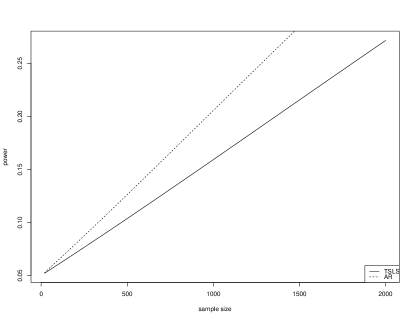
Figure 1: Power curves for the TSLS test statistic and the AR test under different sample sizes (x-axis). The alternative is fixed to be $\beta=0.1$.

Finally, IVsize calculates the minimum sample size needed for achieving a certain power threshold. In the example below, we need a sample size of 3950 for the TSLS test statistic and 2679 for the AR test in order to reject the null in favor of the alternative $\beta=0.1$ with 80% probability.

R> IVsize(cardfit, beta=0.1,power=0.8)
R> IVsize(cardfit, beta=0.1,power=0.8, type="AR")

[1] 5723
[1] 5482

7.3 Diagnostic

Often in an IV analysis, there is concern that the instrument may be invalid. For example, in our dataset, there may be concern that geographic or social features affect both the existence of a nearby 4-year college and earnings of an individual, but not through education. This issue can be seen from the diagnostic plot generated by iv.diagnosis.

R> output <- iv.diagnosis(Y = Y, D = D, Z = Z, X = X)
R> iv.diagnosis.plot(output)

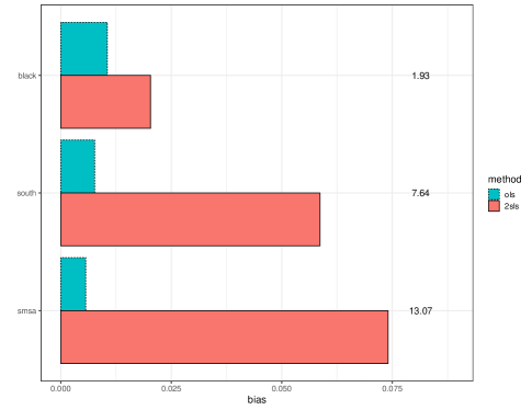
Figure 2: Diagnostic plot for the IV analysis. Each bar in each row represents the magnitude of the bias from not adjusting for a covariate. The number to the right represents the ratio of the biases.

The results are shown in Figure 2. The red and blue bars in Figure 2 are estimated biases using (15) and (16) and the numbers on the right are the ratios between the two biases. The most striking observation from Figure 2 is that the vanilla TSLS estimator would have more than 13 times larger bias than the vanilla OLS estimator if the control potential outcome depends linearly according to (14) on smsa, and the absolute bias would be as large as $0.07$. The bias ratios with respect to south and black are also larger than $1$. We note that these interpretations of Figure 2 depend on the assumptions made in Section 5.1. Specifically, the simplifying assumption (14) that the control potential outcome depends linearly on only one covariate is rather strong, so the diagnostic plot should be interpreted with caveat in mind.

Nevertheless, the diagnostic plot indicates that, without controlling for any covariates, the instrument—proximity to college—is correlated with geographic features such as south and smsa that may also affect the earnings. In particular, if we examine the correlation matrix of the variables below, we see that the geographic features (south and smsa) have much stronger correlation with both the instrument and the outcome than labor force experience (exper and expersq).

R> round(cor(cbind(Z, D, X, Y)), 2)

            Z     D exper expersq black south  smsa     Y
Z        1.00  0.14 -0.06   -0.06 -0.08 -0.22  0.35  0.16
D        0.14  1.00 -0.65   -0.63 -0.27 -0.20  0.19  0.31
exper   -0.06 -0.65  1.00    0.97  0.14  0.11 -0.14  0.01
expersq -0.06 -0.63  0.97    1.00  0.13  0.12 -0.14 -0.02
black   -0.08 -0.27  0.14    0.13  1.00  0.34 -0.04 -0.30
south   -0.22 -0.20  0.11    0.12  0.34  1.00 -0.18 -0.28
smsa     0.35  0.19 -0.14   -0.14 -0.04 -0.18  1.00  0.23
Y        0.16  0.31  0.01   -0.02 -0.30 -0.28  0.23  1.00

Overall, although we can use a TSLS estimator to adjust for these observed covariates like south and smsa, there may well be residual confounding that positively biases the IV analysis. This means the true causal effect of education on earning might not be as large as the estimate from TSLS.

To further illustrate this point, Table 3 compares the OLS and TSLS estimates obtained using ivmodel when different covariates are adjusted for. When only adjusting for exper, expersq, black but not any geographic features, the TSLS estimate is 0.255. This estimate becomes closer to the OLS estimate as the geographic features are included, eventually dropping to 0.132. Both south and smsa are coarse measurements of the geography of survey participants. Had we obtained finer geographic features, the TSLS estimate might be even smaller.

Table 3: A comparison of OLS and TSLS estimates adjusted for different sets of covariates.

	OLS		TSLS
Adjusted covariates	Estimate	Std. error	Estimate	Std. error
None	0.052	0.003	0.188	0.026
exper, expersq, black	0.082	0.004	0.255	0.038
exper, expersq, black, south	0.078	0.004	0.221	0.041
exper, expersq, black, smsa	0.076	0.004	0.177	0.046
exper, expersq, black, south, smsa	0.074	0.004	0.132	0.049

7.4 Sensitivity analysis

We can also perform a sensitivity analysis to assess the sensitivity of our analysis to invalid IV. The user needs to specify the likely range of departure from assumption (A3), captured by the parameter $\delta$ in (18). Roughly speaking, the parameter $\delta\sigma$ captures how much a unit change in the invalid instrument near4c will change the outcome lwage the regression model (18), either through a direct causal effect of near4c on lwage or through correlation of near4c with unincluded determinants of lwage like south.

One way to gauge how large $\delta$ might be is to first fit a standard regression model for the outcome conditional on the education and exogenous covariates.

R> summary(lm(lwage ~ educ + exper + expersq + black + south + smsa,
              data = card.data))

Call:
lm(formula = lwage ~ educ + exper + expersq + black + south +
    smsa, data = card.data)

Residuals:
     Min       1Q   Median       3Q      Max
-1.59297 -0.22315  0.01893  0.24223  1.33190

Coefficients:
              Estimate Std. Error t value Pr(>|t|)
(Intercept)  4.7336643  0.0676026  70.022  < 2e-16 ***
educ         0.0740090  0.0035054  21.113  < 2e-16 ***
exper        0.0835958  0.0066478  12.575  < 2e-16 ***
expersq     -0.0022409  0.0003178  -7.050 2.21e-12 ***
black       -0.1896315  0.0176266 -10.758  < 2e-16 ***
south       -0.1248615  0.0151182  -8.259  < 2e-16 ***
smsa         0.1614230  0.0155733  10.365  < 2e-16 ***
---
Signif. codes:  0 ‘***’ 0.001 ‘**’ 0.01 ‘*’ 0.05 ‘.’ 0.1 ‘ ’ 1

Residual standard error: 0.3742 on 3003 degrees of freedom
Multiple R-squared:  0.2905,    Adjusted R-squared:  0.2891
F-statistic: 204.9 on 6 and 3003 DF,  p-value: < 2.2e-16

Imagine a unmeasured confounder $U$ similar to south, in the sense that $U$ has the same effect on the instrument and the outcome as south. Further, suppose $U$ is independent of the other measured covariates (this is slightly different from south which is weakly correlated with the other covariates). Then we expect the $\delta$ corresponding to such $U$ is about $0.22$ (correlation of south with nearc4) $\times~{}0.12$ (coefficient of south in the regression for lwage) $/~{}0.3742$ (estimated $\sigma$ in the regression for lwage) $\approx 0.07$. Thus, we might assume the range for the sensitivity parameter is $\delta\in(-0.07,0.07)$ to reflect having a covariate like south.

To perform a sensitivity analysis, we can call the function ivmodel specifying the range of the sensitivity parameter.

 R> cardfit.sens =ivmodel(Y=Y, D=D, Z=Z, X=X, deltarange=c(-0.07, 0.07))
 R> summary(cardfit.sens)
  

Anderson-Rubin test:
Sensitivity analysis with deltarange [ -0.07 ,  0.07 ]:
non-central F=6.881108, df1=1, df2=3003, ncp=2.71656, p-value is 0.16499
95 percent confidence interval:
 [ -0.0538384077784691 , 0.53548242970625 ]
  

We see that if there is an unmeasured confounder $U$ that exhibits similar behavior as the variable south, we would retain the null hypothesis of no effect when we use the Anderson-Rubin test statistic. The p-value from the sensitivity analysis is about $0.16$, suggesting that education does not have aa significant positive effect towards earnings if the instrument is invalid due to an unmeasured confounder $U$ with $\Delta$ around 0.07.

We also performed a “synthetic” sensitivity analysis where we intentionally drop the variable south and see if the sensitivity interval in the IV model without south matches the confidence interval in the IV model with south.

R> XwoSouth = X[,c("exper", "expersq", "black","smsa")]
R> cardfit2=ivmodel(Y=Y, D=D, Z=Z, X=XwoSouth, deltarange=c(-0.07, 0.07))
R> summary(cardfit2)

Anderson-Rubin test:
Sensitivity analysis with deltarange [ -0.07 ,  0.07 ]:
non-central F=16.05672, df1=1, df2=3004, ncp=2.785717, p-value is 0.0097825
95 percent confidence interval:
 [ 0.0379720391935471 , 0.513984691572249 ]

Notice that the lower end of this sensitivity interval is nearly identical to the confidence interval for the Anderson-Rubin test that used all the covariates in Section 7.1.

Finally, we can compute the power to detect the favorable alternative under the null hypothesis of no effect, but with a potentially invalid IV. For example, suppose the true effect is $\beta^{*}=0.25$. Then, the power to reject the null of no effect in favor of this alternative with a $\delta\in(-0.07,0.07)$ is 22.7% and we need at least 23,230 samples to increase this power to 80%.

R> IVpower(cardfit.sens, beta=0.25, type="ARsens")
R> IVsize(cardfit3, beta=0.25, power=0.8, type="ARsens")

[1] 0.2265288
[1] 23230

8 Summary

The package ivmodel provides a unified implementation of instrumental variables methods in the case of one endogenous variable. The package contains a general class of estimators, $k$-class estimators, to estimate the parameter $\beta$. The package also contains methods that can deal with violations of instrumental variables assumptions, (A2) and (A3). First, for violations of (A2), the package contains two confidence intervals that are fully robust to weak instruments. For (A3), the package contains methods for sensitivity analysis for the range of violation. Additionally, the package contains power formulas to guide designs of future instrumental variables studies. As our data example in Section 7 demonstrated, our package provides an easy and unified way of conducting a comprehensive instrumental variables analysis with a given data by providing both ways to estimate the parameter of interests, ways to assess the sensitivity of our estimates to violations of IV assumptions, and ways to plan for future IV studies in the form of a power analysis.

Acknowledgments

The research of Hyunseung Kang was supported in part by NSF Grant DMS 1811414.

References

- Amemiya (1985) Takeshi Amemiya. Advanced Econometrics. Harvard University Press, Cambridge, MA, 1985.
- Anderson and Rubin (1949) T. W. Anderson and H. Rubin. Estimation of the parameters of a single equation in a complete system of stochastic equations. The Annals of Mathematical Statistics, 20:46–63, 1949.
- Andrews et al. (2007) D. W. K. Andrews, Marcelo J. Moreira, and James H. Stock. Performance of conditional wald tests in iv regression with weak instruments. Journal of Econometrics, 139(1):116–132, 2007.
- Andrews et al. (2006) Donald W. K. Andrews, Marcelo J. Moreira, and James H. Stock. Optimal two-sided invariant similar tests for instrumental variables regression. Econometrica, 74(3):715–752, 2006.
- Angrist and Krueger (1991) Joshua D. Angrist and Alan B. Krueger. Does compulsory school attendance affect schooling and earnings? The Quarterly Journal of Economics, 106(4):979–1014, 1991.
- Angrist and Krueger (2001) Joshua D. Angrist and Alan B. Krueger. Instrumental variables and the search for identification: From supply and demand to natural experiments. Journal of Economic Perspectives, 15(4):69–85, 2001.
- Angrist et al. (1996) Joshua D. Angrist, Guido W. Imbens, and Donald B. Rubin. Identification of causal effects using instrumental variables. Journal of the American Statistical Association, 91(434):444–455, 1996.
- Baiocchi et al. (2014) Mike Baiocchi, Jing Cheng, and Dylan S. Small. Instrumental variable methods for causal inference. Statistics in Medicine, 33(13):2297–2340, 2014.
- Baum et al. (2003) C. F. Baum, M. E. Schaffer, and S. Stillman. Instrumental variables and gmm: Estimation and testing. Stata Journal, 3(1):1–31, 2003.
- Baum et al. (2007) C. F. Baum, M. E. Schaffer, and S. Stillman. Enhanced routines for instrumental variables/generalized method of moments estimation and testing. Stata Journal, 7(4):465–506, 2007.
- Bollen (2012) Kenneth A. Bollen. Instrumental variables in sociology and the social sciences. Annual Review of Sociology, 38:37–72, 2012.
- Bound et al. (1995) J. Bound, D. A. Jaeger, and R. M. Baker. Problems with instrumental variables estimation when the correlation between instruments and the endogenous variable is weak. Journal of the American Statistical Association, 90:443–450, 1995.