On Conditional Versus Marginal Bias in Multi-Armed Bandits

Abstract

The bias of the sample means of the arms in multi-armed bandits is an important issue in adaptive data analysis that has recently received considerable attention in the literature. Existing results relate in precise ways the sign and magnitude of the bias to various sources of data adaptivity, but do not apply to the conditional inference setting in which the sample means are computed only if some specific conditions are satisfied. In this paper, we characterize the sign of the conditional bias of monotone functions of the rewards, including the sample mean. Our results hold for arbitrary conditioning events and leverage natural monotonicity properties of the data collection policy. We further demonstrate, through several examples from sequential testing and best arm identification, that the sign of the conditional and marginal bias of the sample mean of an arm can be different, depending on the conditioning event. Our analysis offers new and interesting perspectives on the subtleties of assessing the bias in data adaptive settings.

1 Introduction

In modern data analysis, it is often the case that both the data collection and the selection of the target for statistical inference are determined adaptively, i.e. in a manner that depends on the realization of the data observed so far. In these fairly common data-adaptive scenarios, the validity of traditional procedures for statistical inference (that were designed to work in nonadaptive or in i.i.d. settings) can be severely affected.

This issue is perhaps best exemplified within the stochastic multi-armed bandit (MAB) framework (Robbins, 1952). The data are collected sequentially in stages, during which the analyst draws a sample from one among finitely many unknown distributions or arms. At each stage, the determination of whether no more samples are to be acquired (adaptive stopping), the choice of the arm to draw from (adaptive sampling) and the selection of the target arm to analyze once the experiment has terminated (adaptive choosing) are all made based on previously observed data.

The combined effect of these sources of data adaptivity will impact the correctness of standard, nonadaptive statistical procedures in ways that are generally difficult to discern and to quantify. The recent literature on adaptive data analysis in MAB settings has focused primarily on the fundamental problem of mean estimation (Xu et al., 2013; Villar et al., 2015; Bowden & Trippa, 2017; Nie et al., 2018; Shin et al., 2019a). It is now known that the sample mean of an arm is a biased estimator of the true mean and that the sign and magnitude of the bias can be related to adaptive sampling, stopping and choosing in precise ways.

The current theoretical understanding of the bias in MAB experiments is, however limited in two aspects. First, virtually all results concern the bias in mean estimation and do not cover other functionals of the arms. Secondly, and perhaps more interestingly, the existing guarantees cover only the marginal bias of the sample mean, i.e., the bias obtained by accounting for all possible outcomes of the MAB experiment. However, in practice, one is often interested in the sample means of the arms only when certain outcomes have occurred. For instance, the analyst may wish to evaluate the sample mean of a given arm only when that arm was identified as the best arm or, in a sequential framework corresponding to a MAB experiment with only one arm, when the null hypothesis has been rejected or when the random criterion for determining whether enough samples have been collected has been met. In all these cases, it is of interest to compute the conditional bias, i.e., the bias of the sample mean given a certain conditioning event, such as that the arm of interest turned out to be the best arm. A priori, it is not at all clear how the sign of the conditional bias is affected by the choice of the conditioning event and by other sources of data adaptivity (e.g., sampling and stopping), or whether the signs of the marginal and conditional bias should match. See Figure 1 for illustrations of marginal and conditional biases.

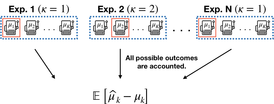
(a) Marginal bias

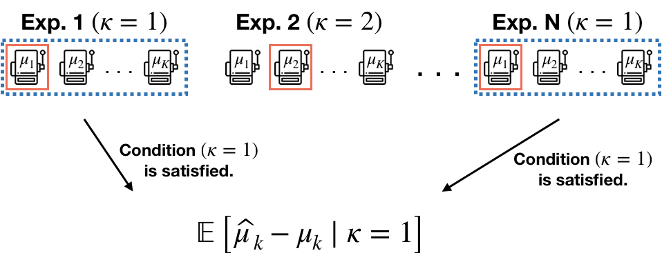
(b) Conditional bias

Figure 1: Illustrations of marginal and conditional biases in the $K$ prototypes example. (a) Marginal bias is obtained by accounting for all possible outcomes. (b) Conditional bias is obtained by accounting for outcomes related to a conditioning event.

As a concrete example, suppose we have $K$ prototypes of an online service and wish to test whether the potential average revenue of each prototype (i.e., arm), $\mu_{k}$, would be larger than a pre-specified threshold $\mu_{0}>0$ based on a stream of test user samples. The usual sequential testing approach will be based on an appropriate upper stopping boundary and will reject each null $\mu_{k}\leq\mu_{0}$ if the corresponding sample mean has crossed such boundary during the testing period. If the null is rejected, then we conclude the prototype as a promising one. If not, we disregard it. It is well known (see, e.g., Starr & Woodroofe, 1968; Shin et al., 2019a) that for each prototype, the sample mean based on data collected through this sequential testing procedure is positively biased: that is, for each $k\in[K]:=\{1,\ldots,K\}$, $\mathbb{E}\left[\widehat{\mu}_{k}\right]\geq\mu_{k}$ regardless of whether the true mean $\mu_{k}$ is larger or smaller than the threshold $\mu_{0}$. This positive bias result can provide a useful warning signal about possible overestimation of the true revenues. At the same time, however, without careful consideration of the conditioning effect, we may end up with a false sense of comfort with low sample mean estimates from “disregarded” prototypes. Indeed, we can naively expect the true revenues of the disregarded prototypes should be even lower than the observed estimates based on the positive bias result $\mathbb{E}\left[\widehat{\mu}_{k}\right]\geq\mu_{k}$. In fact, this would be a wrong conclusion: conditioned on the disregarding event $C$, the sample mean is negatively biased and we have $\mathbb{E}\left[\widehat{\mu}_{k}\mid C\right]\leq\mu_{k}$, as demonstrated in Section 4.1.

In this paper, we make the following contributions:

• We derive in Theorem 2 sufficient conditions for determining the sign of the conditional bias that hold under arbitrary conditioning events and rely on certain natural, highly interpretable monotonicity properties of the rules used for adaptive sampling, stopping and selecting. Our analysis captures in a rigorous and intuitive way the interaction between adaptivity arising from the data collection stage (sampling and stopping) with adaptivity in the choice of the target for inference.

• We characterize the sign of the conditional bias of monotone functions of the rewards of each arm, which includes the sample mean as a special case.

• In Section 4, we demonstrate with several examples in best arm identification and sequential testing problems how the marginal and conditional bias of the sample means of the arms can have opposite signs. These are, we believe, instances of a general, important phenomenon of theoretical and practical relevance.

Overall, our results advance our ability to assess the impact of the bias in adaptive data analysis problems and offer several new and interesting insights on this important issue.

The rest of this paper is organized as follows. In Section 2, we briefly formalize the three notions of adaptivity by introducing a stochastic MAB framework. Section 3 derives results on when the bias can be positive or negative. In Section 4, we demonstrate the correctness of our theoretical predictions through simulations in a variety of practical situations. We end with a brief summary in Section 5, and for reasons of space, we defer all proofs to the Appendix.

2 The Stochastic Multi-Armed Bandit Model

In this section we formally describe the MAB experiment setting, detailing the sources of data adaptivity. Let $P_{1},\dots,P_{K}$ be $K$ distributions of $K$ arms with finite means $\mu_{k}=\int x\mathrm{d}P_{k}(x)$. If it is clear from context, every inequality and equality between two random variables is understood in the almost sure sense.

2.1 Three Sources of Adaptivity in MABs

A general stochastic MAB algorithm consists of the following sampling, stopping, and choosing rules:

• Sampling: For each time $t\geq 1$, choose a possibly randomized index of arm $A_{t}$ from a multinomial distribution $\mathrm{Multi}(1,\nu_{t})\in\{0,1,\dots,K\}$. Then, we draw a sample (also called a reward) $Y_{t}$ from the chosen arm $P_{A_{t}}$. Here, $\nu_{t}\in[0,1]^{K}$ refers to conditional probabilities of sampling each arm defined by

  $$\nu_{t}(k):=\nu_{t}(k\mid\mbox{$\mathcal{D}$}_{t-1})\in[0,1]~{}~{}\forall k\in[K],$$

  with the constraint $\sum_{k=1}^{K}\nu_{t}(k)=1$, and $\mbox{$\mathcal{D}$}_{t-1}$ refers to observed data up to time $t-1$ including all external randomness. If each $\nu_{t}$ does not depend on the previous data $\mbox{$\mathcal{D}$}_{t-1}$, we call it a nonadaptive sampling rule.

  With a proper choice of $\nu_{t}$, this sampling rule captures a broad class of existing methods including fixed design, random allocation, $\epsilon$-greedy (Sutton & Barto, 1998), upper confidence bound (UCB) algorithms (Auer et al., 2002; Audibert & Bubeck, 2009; Garivier & Cappé, 2011; Kalyanakrishnan et al., 2012; Jamieson et al., 2014) and Thompson sampling (Thompson, 1933; Agrawal & Goyal, 2012; Kaufmann et al., 2012).

• Stopping: Given a sampling rule, let $\{\mathcal{F}_{t}\}$ be a filtration such that each $A_{t}$ is $\mbox{$\mathcal{F}$}_{t-1}$-measurable and each $Y_{t}$ and $\mbox{$\mathcal{D}$}_{t}$ are $\mbox{$\mathcal{F}$}_{t}$-measurable. Let $\mathcal{T}$ be a stopping time with respect to the filtration $\{\mathcal{F}_{t}\}$. Then, for each time $t$, the stopping event $\{\mathcal{T}=t\}$ is $\mbox{$\mathcal{F}$}_{t}$-measurable which can be used to characterize a stopping rule of a MAB algorithm.

  For example, the following stopping time corresponds to the stopping rule in which we stop whenever the absolute difference between sample means for arm $1$ and arm $2$ exceeding a fixed threshold $\delta>0$:

  $$\mathcal{T}:=\inf\left\{t\geq 1:\left|\widehat{\mu}_{1}(t)-\widehat{\mu}_{2}(t)\right|>\delta\right\}.$$

  Here, we refer $\widehat{\mu}_{k}(t)$ to the sample mean for arm $k$ defined as

  $$\widehat{\mu}_{k}(t):=\frac{S_{k}(t)}{N_{k}(t)},$$

  where $S_{k}(t)$ and $N_{k}(t)$ are the running sum and number of draws for arm $k$ defined respectively $S_{k}(t):=\sum_{s=1}^{t}\mathbbm{1}(A_{s}=k)Y_{s}$ and $N_{k}(t):=\sum_{s=1}^{t}\mathbbm{1}(A_{s}=k)$ for each $k\in[K]$ and $t\geq 1$. Note that, by the construction, $S_{k}(t)$, $\widehat{\mu}_{k}(t)$ are $\mbox{$\mathcal{F}$}_{t}$-measurable and $N_{k}(t)$ is $\mbox{$\mathcal{F}$}_{t-1}$-measurable for each $k\in[K]$ and $t\geq 1$.

  If a stopping rule is nonadaptive, that is, if the corresponding stopping time is $\mbox{$\mathcal{F}$}_{0}$-measurable, we use $T$ instead of $\mathcal{T}$ to refer the stopping time which includes all fixed time and, more generally, all data-independent stopping rules.

• Choosing: After stopping, let $\mbox{$\mathcal{D}$}_{\mathcal{T}}$ denote collected data up to the stopping time $\mathcal{T}$. Based on $\mbox{$\mathcal{D}$}_{\mathcal{T}}$ with possible randomization, we choose a data-dependent arm based on a choosing rule $\kappa:\mathcal{D}_{\mathcal{T}}\mapsto[K]$. In this paper, we denote the index of chosen arm $\kappa(\mathcal{D}_{\mathcal{T}})$ by $\kappa$ for simplicity.

  For example, in the best arm identification, we often choose the best arm as the arm with the largest sample mean at the stopping time $\mathcal{T}$. In this case, the choosing rule is given as $\kappa=\operatorname*{arg\,max}_{k\in[K]}\widehat{\mu}_{k}(\mathcal{T})$. If $\kappa$ does not depend on the observed data, we call it a nonadaptive choosing rule.

2.2 The Tabular Model of Stochastic MABs

To analyze the theoretical properties of a MAB experiment, it is convenient to express it using an infinite tabular representation of the arm rewards ( Section 2.2 of Shin et al. (2019a), Lattimore & Szepesvári (2019, Section 4.6)).

In the tabular model, we assume that each observation $Y_{t}$ comes from an imaginary $\mathbb{N}\times K$ table or stacks of samples $\{X_{i,k}^{*}\}_{i\in\mathbb{N},k\in[K]}:=X_{\infty}^{*}$ where each $X_{i,k}^{*}$ is an independent draw from $P_{k}$, and the observation $Y_{t}$ is equal to $X_{i,k}^{*}$ if $N_{k}(t)=i$ and $A_{t}=k$ .

Now, given a MAB algorithm, let $W_{t}$ be a random variable which accounts for all possible external randomness of the algorithm for each time $t$. Next, we define $\mbox{$\mathcal{D}$}^{*}_{\infty}=X^{*}_{\infty}\cup\{W_{t}\}_{t=0}^{\infty}$ as the collection of all possible arm rewards and external randomness. Then, given $\mbox{$\mathcal{D}$}_{\infty}^{*}$, every property and outcome of a MAB experiment becomes a deterministic function of $\mbox{$\mathcal{D}$}_{\infty}^{*}$. In particular $\mathcal{T}$, $\kappa$ and $N_{k}(t)$, for each $t$ and $k$, can be expressed as deterministic functions of $\mbox{$\mathcal{D}$}_{\infty}^{*}$. See Section 2.2 in Shin et al. (2019a) for details.

3 Monotonicity Property and Signs of Biases

In a recent work by Shin et al. (2019a), a notion of monotonicity of the data collecting was introduced to characterize the marginal bias of a chosen sample mean at a stopping time. In this section, we summarize the previous result with some minor modifications in notations.

Definition 1.

For each $k\in[K]$, we say a MAB algorithm satisfies the “monotonic increasing (or decreasing) property for arm $k$” if for any $i\in\mathbb{N}$, the function $\mbox{$\mathcal{D}$}^{*}_{\infty}\mapsto\mathbbm{1}\left(\kappa=k\right)/N_{k}(\mathcal{T})$, is an increasing (or decreasing) function of $X_{i,k}^{*}$ while keeping all other entries in $\mbox{$\mathcal{D}$}^{*}_{\infty}$ fixed. Further, we say that

• A sampling rule is optimistic for arm $k$ if the function $\mbox{$\mathcal{D}$}^{*}_{\infty}\mapsto N_{k}(t)$ is an increasing function of $X_{i,k}^{*}$ while keeping all other entries in $\mbox{$\mathcal{D}$}^{*}_{\infty}$ fixed for any fixed $i\in\mathbb{N}$ and $t\geq 1$;

• A stopping rule is optimistic for arm $k$ if the function $\mbox{$\mathcal{D}$}^{*}_{\infty}\mapsto\mathcal{T}$ is a decreasing function of $X_{i,k}^{*}$ while keeping all other entries in $\mbox{$\mathcal{D}$}^{*}_{\infty}$ fixed for any fixed $i\in\mathbb{N}$;

• A choosing rule is optimistic for arm $k$ if the function $\mbox{$\mathcal{D}$}^{*}_{\infty}\mapsto\mathbbm{1}(\kappa=k)$ is an increasing function of $X_{i,k}^{*}$ while keeping all other entries in $\mbox{$\mathcal{D}$}^{*}_{\infty}$ fixed for any fixed $i\in\mathbb{N}$.

It can be shown that many MAB algorithms, including $\epsilon$-greedy, UCB, and Thompson sampling algorithms, have optimistic sampling rules. As for optimistic stopping, a sequential testing procedure with an upper stopping boundary yields a typical example of an optimistic stopping rule based on the stopping time $\mathcal{T}:=\inf\left\{t:\widehat{\mu}(t)>U(t)\right\}$ where $t\mapsto U(t)$ is a deterministic function characterizing the upper stopping boundary. Finally, the index of the arm with the largest sample mean, $\kappa=\operatorname*{arg\,max}_{k\in[K]}\widehat{\mu}_{k}(\mathcal{T})$ can be viewed as a typical optimistic choosing rule.

3.1 The Sign of the Marginal Bias

Shin et al. (2019a) demonstrated how certain natural monotonicity properties of the MAB experiment can be exploited to determine the sign of the marginal bias and of the conditional bias given conditioning events corresponding to adaptive choosing of arms. For completeness, we recall this result next.

Proposition 1 (Theorem 7 in Shin et al. (2019a)).

Given a MAB algorithm, suppose we have $\mathbb{E}\left[N_{k}(\mathcal{T})\right]<\infty$ and $N_{k}(\mathcal{T})\geq 1$ for all $k$ with $\mathbb{P}\left(\kappa=k\right)>0$. If the MAB algorithm satisfies the monotonic decreasing property for each arm $k$ with $\mathbb{P}\left(\kappa=k\right)>0$ then we have

$$\mbox{$\mathbb{E}$}\left[\widehat{\mu}_{k}(\mathcal{T})\mid\kappa=k\right]\leq\mu_{k},$$ (1)

which also also implies that

$$\mbox{$\mathbb{E}$}\left[\widehat{\mu}_{\kappa}(\mathcal{T})-\mu_{\kappa}\right]\leq 0.$$ (2)

Similarly if the MAB algorithm satisfies the monotonic increasing property for each arm $k$ with $\mathbb{P}\left(\kappa=k\right)>0$ then we have

$$\mbox{$\mathbb{E}$}\left[\widehat{\mu}_{k}(\mathcal{T})\mid\kappa=k\right]\geq\mu_{k},$$ (3)

which also implies that

$$\mbox{$\mathbb{E}$}\left[\widehat{\mu}_{\kappa}(\mathcal{T})-\mu_{\kappa}\right]\geq 0.$$ (4)

If each arm has a bounded distribution then the condition $\mathbb{E}\left[N_{k}(\mathcal{T})\right]<\infty$ can be dropped.

Note that if a MAB algorithm consists of an optimistic sampling but nonadaptive stopping and choosing rules, then the algorithm satisfies the monotonic decreasing property. This is the reason why $\epsilon$-greedy, UCB, and Thompson sampling algorithms yield a negatively biased sample mean for each arm, marginally.

Also, if a MAB algorithm consists of an optimistic stopping but nonadaptive sampling and choosing, the algorithm satisfies the monotonic increasing property, which explains why sequential testing procedures (corresponding to one-arm MBA experiments) with an upper stopping boundary produces a positively biased sample mean.

3.2 The Sign of the Conditional Bias

In this section, we generalize Proposition 1 and derive sufficient conditions for the sign of the conditional bias under arbitrary conditioning events of monotone functions of the arms rewards.

We first introduce some notation. For each arm $k$, let $F_{k}$ denote the corresponding cumulative distribution function (CDF): $y\in\mathbb{R}\mapsto F_{k}(y)=\mathbb{P}(X\leq y),$ where $X\sim P_{k}$. Let $\widehat{F}_{k,t}$ be the empirical CDF for arm $k$ based on samples up to time $t$; that is, $\widehat{F}_{k,t}$ is a random function on $\mathbb{R}$ and taking values in $[0,1]$ given by

$$y\in\mathbb{R}\mapsto\widehat{F}_{k,t}(y):=\frac{1}{N_{k}(t)}\sum_{s=1}^{t}\mathbbm{1}\left(A_{s}=k,Y_{s}\leq y\right),$$ (5)

which returns the fractions of samples from arm $k$ whose values are no larger than $y$. For a stopping time $\mathcal{T}$ with respect to the MAB filtration $\{\mathcal{F}_{t}\}$, we then define $\widehat{F}_{k,\mathcal{T}}$ to be the empirical CDF of the rewards of arm $k$ up to time $\mathcal{T}$; that is, for each $y\in\mathbb{R}$,

$$\widehat{F}_{k,\mathcal{T}}(y):=\lim_{t\to\infty}\widehat{F}_{k,\mathcal{T}\wedge t}(y).$$

The use of the limit in the above definition is a necessary technicality in order to allow for the possibility that $\mathcal{T}=\infty$. Note that, on the event $\{N_{k}(\mathcal{T})=\infty\}=\{\lim_{t\to\infty}N_{k}(\mathcal{T}\wedge t)=\infty\}$, we have that, for each $y\in\mathbb{R}$, $\widehat{F}_{k}(y)=F_{k}(y)$ almost surely, based on the strong law of large numbers; see Theorem 2.1 in Gut (2009).

Next, for any function $f:\mathbb{R}\to\mathbb{R}$ integrable with respect to $P_{k}$, let $E_{k}f=\int f(x)\mathrm{d}P_{k}(x)$ be the corresponding expectation. Similarly, we let

$$\widehat{E}_{k,t}f=\frac{1}{N_{k}(t)}\sum_{s=1}^{t}f(Y_{s})\mathbbm{1}\left(A_{s}=k\right)$$

to be the expectation of $f$ under the empirical measure of the $k$-th arm at time $t$. Clearly, $\widehat{E}_{k,t}f$ is a random variable. If $f$ is the identity function, then it is immediate to see that $E_{k}f=\mu_{k}$ and $\widehat{E}_{k,t}f=\widehat{\mu}_{k}(t)$. Also, for any $y\in\mathbb{R}$, setting $f$ to be the indicator function $x\mapsto f(x)=\mathbbm{1}(x\leq y)$ yields that $E_{k}f=F_{k}(y)$ and $\widehat{E}_{k,t}f=\widehat{F}_{k,t}(y)$. Finally, for a (possibly infinite) stopping time $\mathcal{T}$ with respect to the filtration $\{\mathcal{F}_{t}\}$, we set

$$\widehat{E}_{k,\mathcal{T}}f=\lim_{t\rightarrow\infty}\widehat{E}_{k,\mathcal{T}\wedge t}f.$$

We are now ready to present the main result of this paper. The proof is given in Section A.1. For any event $C$, we let $\mathbb{E}[\cdot|C]$ denote the conditional expectation given $C$.

Theorem 2.

Let $\mathcal{T}$ be a stopping time with respect to the MAB experiment natural filtration $\{\mathcal{F}_{t}\}$. For a fixed $k\in[K]$, suppose $N_{k}(\mathcal{T})\geq 1$. Let $C\in\mathcal{F}_{\mathcal{T}}$ be any event at stopping time $\mathcal{T}$ with $\mathbb{P}(C)>0$. Assume that, for each $i$, the function $\mbox{$\mathcal{D}$}^{*}_{\infty}\mapsto\mathbbm{1}\left(C\right)/N_{k}(\mathcal{T})$ is a decreasing function of $X_{i,k}^{*}$ while keeping all other entries in $\mbox{$\mathcal{D}$}^{*}_{\infty}$ fixed. Then, for each $y\in\mathbb{R}$,

$$\inf_{y\in\mathbb{R}}\left(\mbox{$\mathbb{E}$}\left[\widehat{F}_{k,\mathcal{T}}(y)\mid C\right]-F_{k}(y)\right)\geq 0,$$ (6)

or, equivalently, for any non-decreasing function $f:\mathbb{R}\to\mathbb{R}$ with $\mbox{$\mathbb{E}$}\left[\widehat{E}_{k,\mathcal{T}}|f|\mid C\right]<\infty$ and $E_{k,\mathcal{T}}|f|<\infty$,

$$\mbox{$\mathbb{E}$}\left[\widehat{E}_{k,\mathcal{T}}f\mid C\right]\leq E_{k}f.$$ (7)

Similarly, if, for each $i$, the function $\mbox{$\mathcal{D}$}^{*}_{\infty}\mapsto\mathbbm{1}\left(C\right)/N_{k}(\mathcal{T})$ is an increasing function of $X_{i,k}^{*}$ while keeping all other entries in $\mbox{$\mathcal{D}$}^{*}_{\infty}$ fixed, then we have

$$\sup_{y\in\mathbb{R}}\left(\mbox{$\mathbb{E}$}\left[\widehat{F}_{k,\mathcal{T}}(y)\mid C\right]-F_{k}(y)\right)\leq 0,$$ (8)

or, equivalently,

$$\mbox{$\mathbb{E}$}\left[\widehat{E}_{k,\mathcal{T}}f\mid C\right]\geq E_{k}f,$$ (9)

for any non-decreasing function $f:\mathbb{R}\to\mathbb{R}$ satisfying $\mbox{$\mathbb{E}$}\left[\widehat{E}_{k,\mathcal{T}}|f|\mid C\right]<\infty$ and $E_{k,\mathcal{T}}|f|<\infty$.

The important conclusion from the above theorem is that the conditional expected value of the empirical CDF of the rewards of any given arm can be stochastically smaller or greater than the true CDF of the corresponding arm. And furthermore, the sign of the bias can be determined in the basis of natural and often verifiable (as shown below) monotonicity conditions that depend on (i) the specific sampling and stopping rules deployed in the MAB experiment and (ii) the choice of the conditioning event $C$.

Note that if in the theorem we choose $C$ as the conditioning event $\{\kappa=k\}$ and the function $f$ as the identity function, Theorem 2 yields Proposition 1 of Shin et al. (2019a) as a special case (indeed the statements about the marginal bias in that result follows from those on the conditional bias given the conditioning event $\{\kappa=k\}$). We emphasize that Theorem 2 is a generalization of Proposition 1 of Shin et al. (2019a) in at least two ways: (i) it provides a more general guarantee about the conditional bias of monotone functions of the empirical CDF of the arms as opposed to just the sample mean and (ii) it allows for virtually any conditioning event that depends on the outcome of the MAB experiment (formally, that is measurable with respect to $\mathcal{F}_{\mathcal{T}})$.

The monotonicity assumption in Theorem 2 captures in a mathematically concise yet intuitive manner how adaptivity in the data collection process combines with adaptivity in the selective data analysis, exemplified by the conditioning event, to affect the sign of the bias. The interaction between these two sources of adaptivity is, at least to us, not at all apparent and, in fact, rather subtle. To illustrate this phenomenon, in the next section, we apply Theorem 2 in several, fairly routine, situations in adaptive data analysis to demonstrates how marginal and conditional biases may very well have opposite signs.

4 Applications

In this section, we discuss several practical examples of the conditional bias results in Theorem 2.

4.1 Conditional Versus Marginal Bias of a Stopped Sequential Test

Suppose we have a stream of samples from a single arm with a finite mean $\mu$. For each $t$, let $\widehat{\mu}(t)$ be the sample mean of the rewards observed up to time $t$.

To test whether $\mu$ is larger than a reference value $\mu_{0}$, we may construct an upper boundary $t\mapsto U(t)$ and conclude that $\mu\geq\mu_{0}$ if the sample mean ever crosses the upper boundary.

Let $\mathcal{T}$ be the first time the sample mean crosses the boundary, i.e. $\mathcal{T}:=\inf\left\{t\geq 1:\widehat{\mu}(t)\geq U(t)\right\}$. The stopping time $\mathcal{T}$ is an example of an optimistic stopping and, from Proposition 1, we can check that the stopped sample mean $\widehat{\mu}(\mathcal{T})$ is always positively biased (Shin et al., 2019a).

However, the stopping time $\mathcal{T}$ can be large or even infinite with non-zero probability. Thus, in practice, we may want to allow for the possibility of stopping the sequential test before reaching the stopping time. Let $M$ be any fixed predefined time at which we stop the testing procedure (if still ongoing), and let $\mathcal{T}_{M}:=\min\left\{\mathcal{T},M\right\}$ be the corresponding stopping time which takes account the early stopping option. Again, by Proposition 1, we know that the stopped sample mean $\widehat{\mu}(\mathcal{T}_{M})$ is still positively biased, i.e. $\mathbb{E}\left[\widehat{\mu}(\mathcal{T}_{M})\right]\geq\mu,$ since the function $\mbox{$\mathcal{D}$}_{\infty}^{*}\mapsto 1/\mathcal{T}_{M}$ is an increasing function of $X_{i}^{*}$ while keeping all other entries in $\mbox{$\mathcal{D}$}_{\infty}^{*}$ fixed. From Theorem 2, we can also check that the expected empirical CDF at stopping time $\mathcal{T}_{M}$ is negatively biased:

$$\sup_{y\in\mathbb{R}}\left(\mbox{$\mathbb{E}$}\left[\widehat{F}_{k,\mathcal{T}_{M}}(y)\right]-F_{k}(y)\right)\leq 0.$$ (10)

Conditioned on the early stopping event $\{M<\mathcal{T}\}$, however, Theorem 2 shows that the early stopped sample mean and the empirical CDF are negatively and positively biased, respectively, since the function $\mbox{$\mathcal{D}$}_{\infty}^{*}\mapsto\frac{\mathbbm{1}(M<\mathcal{T})}{\mathcal{T}_{M}}=\frac{\mathbbm{1}(M<\mathcal{T})}{M}$ is an decreasing function of $X_{i}^{*}$ while keeping all other entries in $\mbox{$\mathcal{D}$}_{\infty}^{*}$ fixed. That is,

$$\mathbb{E}\left[\widehat{\mu}(M)\mid M<\mathcal{T}\right] \leq\mu,$$ (11)

$$\inf_{y\in\mathbb{R}}\left(\mbox{$\mathbb{E}$}\left[\widehat{F}_{k,M}(y)\mid M<\mathcal{T}\right]-F_{k}(y)\right) \geq 0.$$ (12)

However, we can also check that the function $\mbox{$\mathcal{D}$}_{\infty}^{*}\mapsto\frac{\mathbbm{1}(M\geq\mathcal{T})}{\mathcal{T}_{M}}=\frac{\mathbbm{1}(M\geq\mathcal{T})}{\mathcal{T}}$ is an increasing function of $X_{i}^{*}$, which implies that, on the line-crossing event $\left\{M\geq\mathcal{T}\right\}$, the sample mean and empirical CDF are positively and negatively biased, respectively. Thus, depending on the conditioning event, the conditional bias can be positive or negative. Also note that, without the early stopping condition, $\widehat{\mu}(M)$ is an unbiased estimator of $\mu$.

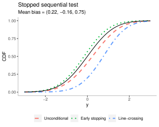
Figure 2: Average of marginal (red dashed line) and conditional empirical CDFs (green dotted and blue dot-dashed lines) from repeated stopped sequential test in Section 4.1. The black solid line refers to the true CDF of the underlying arm

Experiment: We verify these facts with simulations, where we repeat a stopped sequential test $10^{5}$ times. In each test, the arm corresponds to a standard normal distribution, and the upper boundary is constructed by the point-wise upper confidence bounds $t\mapsto U(t)=\frac{z_{\alpha}}{\sqrt{t}}$, where $z_{\alpha}$ is the $\alpha$-upper quantile of the standard normal distribution. Note that this upper boundary does not yield a valid testing procedure since it inflates the type 1 error. However, we choose this boundary with unusual parameters $\alpha=0.2$ and $M=10$ to manifest the difference between marginal and conditional biases.

Figure 2 shows the point-wise averages of the observed marginal and conditional CDFs from the simulated $10^{5}$ stopped sequential tests. The black solid line refers to the true CDF of the underlying arm. The red dashed line corresponds to the marginal CDF, which lies below the true CDF, as expected, and thus the corresponding mean bias is positive. The green dotted and blue dot-dashed lines correspond to the averages of empirical CDFs conditioned on the early stopping and line-crossing events, respectively. As predicted, conditioned on the early stopping event, the empirical CDF and the sample mean are positively and negatively biased, respectively. In contrast, conditioned on the line-crossing event, the empirical CDF and the sample mean are negatively and positively biased, respectively.

4.2 Sequential Test for Two Arms: Conditional Biases from Upper and Lower Stopping Boundaries

Suppose we have two independent arms with unknown means $\mu_{1}$ and $\mu_{2}$. In this subsection, we consider the following testing problem:

$$H_{0}:\mu_{1}\leq\mu_{2}~{}~{}\text{vs}~{}~{}H_{1}:\mu_{1}>\mu_{2}.$$ (13)

To test this hypothesis, we draw a sample from arm $1$ for every odd time and from arm $2$ for every even time. Then, at each even time $t$, we check whether the difference between the sample means $\widehat{\mu}_{1}(t)$, $\widehat{\mu}_{2}(t)$ from the two arms crosses predefined upper and lower stopping boundaries, $t\mapsto U(t)$ and $t\mapsto L(t)$.

To be specific, define stopping times $\mathcal{T}^{U}$ and $\mathcal{T}^{L}$ as follows:

$$\mathcal{T}^{U} :=\inf\left\{t\in\mathbb{N}_{\mathrm{even}}:\widehat{\mu}_{1}(t)-\widehat{\mu}_{2}(t)\geq U(t)\right\},$$ (14)

$$\mathcal{T}^{L} :=\inf\left\{t\in\mathbb{N}_{\mathrm{even}}:\widehat{\mu}_{1}(t)-\widehat{\mu}_{2}(t)\leq L(t)\right\}.$$ (15)

Let $M>0$ be a predetermined maximum time budget. Based on $\mathcal{T}^{U},\mathcal{T}^{L}$ and $M$, we stop sampling whenever $\widehat{\mu}_{1}(t)-\widehat{\mu}_{2}(t)$ crosses one of the boundaries or the maximum time budget $M$ is met. Define the corresponding stopping time as $\mathcal{T}_{M}:=\min\left\{\mathcal{T}^{U},\mathcal{T}^{L},M\right\}$. At time $\mathcal{T}_{M}$, we accept $H_{1}$ if $\mathcal{T}_{M}=\mathcal{T}^{U}$ (upper-crossing event), and accept $H_{0}$ if $\mathcal{T}_{M}=\mathcal{T}^{L}$ (lower-crossing event). Otherwise, we declare that we do not have enough evidence to accept either one of two hypotheses.

In this case, we cannot apply Proposition 1 to determine the sign of the marginal bias since the stopping rule is neither optimistic nor pessimistic, marginally. However, we can determine the sign of the conditional bias based on Theorem 2 since the the function $\mbox{$\mathcal{D}$}_{\infty}^{*}\mapsto\frac{\mathbbm{1}(\mathcal{T}^{U}\leq\min\left\{\mathcal{T}^{L},M\right\})}{\mathcal{T}^{U}}$ is an increasing (resp. decreasing) function of $X_{i,1}^{*}$ (resp. $X_{i,2}^{*}$) for each $i$, keeping all other entries in $\mbox{$\mathcal{D}$}_{\infty}^{*}$ fixed.

In detail, conditioned on the event of accepting $H_{0}$, the sample mean and empirical CDF for arm $1$ are negatively and positively biased, respectively. That is,

$$\mathbb{E}\left[\widehat{\mu}_{1}(\mathcal{T}_{M})\mid\mathcal{T}_{M}=\mathcal{T}^{L}\right]$$

$$=\mathbb{E}\left[\widehat{\mu}_{1}(\mathcal{T}^{L})\mid\mathcal{T}^{L}\leq\min\left\{\mathcal{T}^{U},M\right\}\right]\leq\mu_{1},$$ (16)

$$\inf_{y\in\mathbb{R}}\left(\mbox{$\mathbb{E}$}\left[\widehat{F}_{k,\mathcal{T}_{M}}(y)\mid\mathcal{T}_{M}=\mathcal{T}^{L}\right]-F_{k}(y)\right)$$

$$=\inf_{y\in\mathbb{R}}\left(\mbox{$\mathbb{E}$}\left[\widehat{F}_{k,\mathcal{T}^{L}}(y)\mid\mathcal{T}^{L}\leq\min\left\{\mathcal{T}^{U},M\right\}\right]-F_{k}(y)\right)$$

$$\geq 0.$$ (17)

Similarly, for arm 2, we have opposite signs of the sample mean and empirical CDF.

By the same reasoning, the signs of the conditional biases conditioned on the event of accepting $H_{1}$ are reversed:

$$\mathbb{E}\left[\widehat{\mu}_{1}(\mathcal{T}_{M})\mid\mathcal{T}_{M}=\mathcal{T}^{U}\right]$$

$$=\mathbb{E}\left[\widehat{\mu}_{1}(\mathcal{T}^{U})\mid\mathcal{T}^{U}\leq\min\left\{\mathcal{T}^{L},M\right\}\right]\geq\mu_{1},$$ (18)

$$\sup_{y\in\mathbb{R}}\left(\mbox{$\mathbb{E}$}\left[\widehat{F}_{k,\mathcal{T}_{M}}(y)\mid\mathcal{T}_{M}=\mathcal{T}^{U}\right]-F_{k}(y)\right)$$

$$=\sup_{y\in\mathbb{R}}\left(\mbox{$\mathbb{E}$}\left[\widehat{F}_{k,\mathcal{T}^{U}}(y)\mid\mathcal{T}^{U}\leq\min\left\{\mathcal{T}^{L},M\right\}\right]-F_{k}(y)\right)$$

$$\leq 0.$$ (19)

Thus, we conclude that, in all cases, the expected difference between the sample means are exaggerated toward “the direction of decision”.

Remark 3.

These results hold regardless of whether the underlying distribution is under the null or alternative.

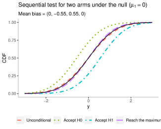
Figure 3: Average of marginal and conditional empirical CDFs of arm 1 from repeated sequential tests for two arms in Section 4.2. The black solid line refers to the true CDF of the underlying arm.

Experiment: To demonstrate the conditional bias result, we set two standard normal arms with same means $\mu_{1}=\mu_{2}=0$. In this experiment, we use upper and lower stopping boundaries based on naive point-wise confidence intervals:

$$U(t):=z_{\alpha/2}\sqrt{\frac{2}{t}},\quad\text{and}\quad L(t)=-U(t),$$ (20)

where $\alpha$ is set to $0.2$ to show the bias better. Figure 3 show the marginal and conditional biases of the empirical CDFs and sample means for arm $1$ based on $10^{5}$ repetitions of the experiment. The black solid line corresponds to the true underlying CDF. The red dashed line refers to the average of the marginal CDFs, and the purple long-dashed line corresponds to the average of the empirical CDFs conditioned on reaching the maximal time. Note that for these two cases, the empirical CDFs are neither positively nor negatively biased across all $y\in\mathbb{R}$.

However, for the cases corresponding to accepting $H_{0}$ (green dotted line) and accepting $H_{1}$ (blue dot-dashed line), the empirical CDFs are positively and negatively biased, respectively: see inequalities (17) and  (19). The conditional bias of the sample mean is also negative conditioning on the event of accepting $H_{0}$ and positive conditioning on the event of accepting $H_{1}$: see inequalities (16) and  (18).

4.3 Best-Arm Identification: (i) lil’UCB Algorithm

Suppose we have $K>2$ sub-Gaussian arms with a common and known parameter $\sigma^{2}$. In many applications, we may want to identify which of the $K$ arms has the largest mean parameter by using as few samples as possible.

In the previous subsection, we observed that, in the two-armed bandit setting, if we use a boundary-crossing compatible with a best-arm identification style algorithm with deterministic sampling, then the optimal arm has positive bias and the sub-optimal arm has a negative bias.

Shin et al. (2019a) showed that the same phenomenon happens for the best arm as chosen by the lil’UCB algorithm, which consists of the following sampling, stopping and choosing rules (Jamieson et al., 2014):

• Sampling: For $t=1,\dots K$, draw a sample from each arm. For $t>K$, draw a sample from arm $k$ if

  $$k=\operatorname*{arg\,max}_{j\in[K]}\widehat{\mu}_{j}(t-1)+u^{\text{lil}}\left(N_{j}(t-1)\right),$$

  where $\beta,\epsilon,\lambda>0$ and $\delta>0$ are algorithm parameters and

  $$u^{\text{lil}}\left(n\right):= (1+\beta)(1+\sqrt{\epsilon})$$

  $$\times\sqrt{2\sigma^{2}(1+\epsilon)\log\left(\log((1+\epsilon)n)/\delta\right)/n}.$$

• Stopping: the stopping time $\mathcal{T}$ is defined as the first time at which the following inequality holds for some $k\in[K]$:

  $$N_{k}(t)\geq 1+\lambda\sum_{j\neq k}N_{j}(t),$$

  where $\lambda>0$ is an algorithm parameter.

• Choosing: $\kappa=\operatorname*{arg\,max}_{k\in[K]}N_{k}(\mathcal{T})$.

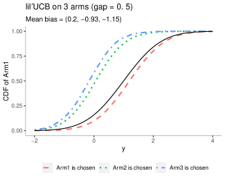
Figure 4: Average of conditional empirical CDFs of arm 1 from $10^{5}$ lil’UCB algorithm runs on three unit-variance normal arms with $\mu_{1}=1,\mu_{2}=0.5$ and $\mu_{3}=0$, as described in Section 4.3. The black solid line refers to the true CDF of arm 1.

Proposition 4 (Corollary 8 in Shin et al. (2019a)).

In the settings of the lil’UCB algorithm, for each $k$ with $\mathbb{P}(\kappa=k)>0$, we have that

$$\mathbb{E}\left[\widehat{\mu}_{k}(\mathcal{T})\mid\kappa=k\right]\geq\mu_{k}.$$ (21)

The following corollary to Theorem 2 shows a complementary result—the sample mean and the empirical CDF of a given arm are negatively and positively biased, respectively, conditioned on the event that the arm is not selected as the best arm. In contrast, on the same conditioning event, the empirical distribution of the selected arm is negatively biased.

Corollary 5.

In the settings of the lil’UCB algorithm, for each $k$ with $\mathbb{P}(\kappa\neq k)>0$, we have that

$$\mathbb{E}\left[\widehat{\mu}_{k}(\mathcal{T})\mid\kappa\neq k\right] \leq\mu_{k},$$ (22)

$$\inf_{y\in\mathbb{R}}\left(\mbox{$\mathbb{E}$}\left[\widehat{F}_{k,\mathcal{T}}(y)\mid\kappa\neq k\right]-F_{k}(y)\right) \geq 0.$$ (23)

Also, for each $k$ with $\mathbb{P}(\kappa=k)>0$,

$$\mathbb{E}\left[\widehat{\mu}_{k}(\mathcal{T})\mid\kappa=k\right] \geq\mu_{k},$$ (24)

$$\sup_{y\in\mathbb{R}}\left(\mbox{$\mathbb{E}$}\left[\widehat{F}_{k,\mathcal{T}}(y)\mid\kappa=k\right]-F_{k}(y)\right) \leq 0.$$ (25)

The proof of Corollary 5 can be found in Section A.2.

Remark 6.

Corollary 5 remains true for any other choice of $u^{\text{lil}}$ if the function $n\mapsto u^{\text{lil}}(n)$ is decreasing.

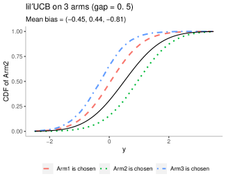
Figure 5: Average of conditional empirical CDFs of arm 2 from $10^{5}$ lil’UCB algorithm runs on three unit-variance normal arms with $\mu_{1}=1,\mu_{2}=0.5$ and $\mu_{3}=0$, as described in Section 4.3. The black solid line refers to the true CDF of arm 2.

Experiment: To verify the previous claims, we conducted $10^{5}$ trials of the lil’UCB algorithm on three unit-variance normal arms with $\mu_{1}=1,\mu_{2}=0.5$ and $\mu_{3}=0$. It is important to note that the signs of the biases do not depend on the choice of parameters or of the underlying distributions, but the magnitudes of the biases do. To best illustrates the bias results, we use an unusual set of algorithm parameters as $\delta=0.2$, $\epsilon=0.1$, $\beta=0.5$ and $\lambda=1$ in this experiment.

Figure 4 shows the averages of the empirical CDFs of arm 1 (the arm with the larges mean) conditioned on each arm being chosen as the best arm. The black solid line corresponds to the true underlying CDF. The red dashed line, which lies below the true CDF, indicates that the empirical CDF of arm 1 conditioned on the event that the arm 1 is chosen as the best arm (i.e., $\kappa=1$) is negatively biased; this then implies that the sample mean of the chosen arm is positively biased. In contrast, the green dotted and blue dot-dashed lines, lying above the true CDF, show that conditioned on the event the arm 1 is not chosen as the best arm (i.e., $\kappa\neq 1$), the empirical CDF is positively biased and the sample mean is negatively biased.

Figure 5 displays the averages of the empirical CDFs of arm 2. Though arm 2 is not the best arm, we can check that the signs of the conditional biases follow the same pattern as arm 1. Conditioned on the event that arm 2 is chosen as the best arm ($\kappa=2$), the empirical CDF is negatively biased (green dotted line), but conditioned on the event that arm 2 is not chosen as the best arm ($\kappa\neq 2)$, the corresponding CDFs are now positively biased (red dashed and blue dot-dashed lines), as expected.

4.4 Best-Arm Identification: (ii) Sequential Halving

The action elimination (Paulson et al., 1964; Even-Dar et al., 2002, 2006; Karnin et al., 2013) is another class of best arm identification algorithms in which each arm in an active set is sampled a fixed number of times and some of arms are eliminated from the active set at each round. In this subsection, we focus on the sequential halving algorithm (Karnin et al., 2013), which is designed to identify the best arm with high probability and based on a fixed number of samples. To be specific, the sequential halving algorithm for a given time budget $T$ is defined as follows :

• Initialize the set of active arms $\mbox{$\mathcal{A}$}_{1}=[K]$.

• In each round $r=1,\dots,\lceil\log_{2}K\rceil$, for each arm $k$ in $\mbox{$\mathcal{A}$}_{r}$, draw

  $$m_{r}:=\left\lfloor\frac{T}{|\mbox{$\mathcal{A}$}_{r}|\lceil\log_{2}K\rceil}\right\rfloor$$

  i.i.d. samples from it, and let $\widehat{\mu}_{k}^{(r)}$ be the average of the observed samples in the round.

• Let $\mathcal{A}_{r+1}$ be the set of $\left\lceil|\mbox{$\mathcal{A}$}_{r}/2|\right\rceil$ arms in $\mbox{$\mathcal{A}$}_{r}$ with the largest average based on data collected in round $r$.

• Choose the unique arm in $\mbox{$\mathcal{A}$}_{\lceil\log_{2}K\rceil+1}$ as the best one.

Let $\kappa$ be the (random) index of the chosen arm at the final time $T$, and for each $k\in[K]$, let $\widehat{\mu}_{k}(T)$ be the sample mean of arm $k$ at time $T$ based on all previously collected $N_{k}(T)$ samples from that arm.

The following two corollaries show that under the sequential halving algorithm, the sample mean and empirical CDF of each arm is negatively and positively biased, respectively, marginally and conditionally on the event that the arm is not selected as the best one ($\kappa\neq k$). On the other hand, conditionally on the event that the arm is selected as the best one ($\kappa=k$), the sample mean and empirical CDF of each arm is positively and negatively biased, respectively.

Corollary 7.

Suppose that data are collected by the sequential halving algorithm with a time budget $T$. Then, for each $k\in[K]$ and for each $t\leq T$, we have that

$$\mathbb{E}\left[\widehat{\mu}_{k}(t)\right] \leq\mu_{k},$$ (26)

$$\inf_{y\in\mathbb{R}}\left(\mbox{$\mathbb{E}$}\left[\widehat{F}_{k,t}(y)\right]-F_{k}(y)\right) \geq 0.$$ (27)

Corollary 8.

In the settings of the sequential halving algorithm with a time budget $T$, for each $k$ with $\mathbb{P}(\kappa\neq k)>0$, we have that

$$\mathbb{E}\left[\widehat{\mu}_{k}(T)\mid\kappa\neq k\right] \leq\mu_{k},$$ (28)

$$\inf_{y\in\mathbb{R}}\left(\mbox{$\mathbb{E}$}\left[\widehat{F}_{k,T}(y)\mid\kappa\neq k\right]-F_{k}(y)\right) \geq 0.$$ (29)

Also, for each $k$ with $\mathbb{P}(\kappa=k)>0$,

$$\mathbb{E}\left[\widehat{\mu}_{k}(T)\mid\kappa=k\right] \geq\mu_{k},$$ (30)

$$\sup_{y\in\mathbb{R}}\left(\mbox{$\mathbb{E}$}\left[\widehat{F}_{k,T}(y)\mid\kappa=k\right]-F_{k}(y)\right) \leq 0.$$ (31)

The proofs of Corollary 7 and 8 can be found in Section A.3. Due to limited space, an experiment about the bias of the sequential halving algorithm is presented in Section B.2.

5 Summary

In this paper, we have investigated the sign of the conditional bias of monotone functions of the rewards in the MAB framework under an arbitrary conditioning event, generalizing the results in Shin et al. (2019a), and complementing the results on the magnitude of the bias (Shin et al., 2019b). In our analysis, we have exploited certain natural monotonicity properties of MAB experiments and have characterized the impact on the bias of both adaptivity in the data acquisition process and in the selection of the target for inference.

Several interesting extensions of our results are worth pursuing. We emphasize two important ones:

• It is still an open problem how to characterize the bias (marginal or conditional) of other important functionals that are not necessarily monotone or linear, such as the sample variance and sample quantiles.

• Several debiasing methods have been proposed in the MAB literature: see, e.g., Xu et al. (2013); Deshpande et al. (2018); Neel & Roth (2018); Nie et al. (2018); Hadad et al. (2019). However, the existing approaches typically only adjust for adaptive sampling but ignore the other sources of adaptivity. Current debiasing methods do not offer theoretical guarantees at stopping times, and also do not account for natural conditioning events in MABs, like selection of a promising arm. Furthermore, they are typically not interested in characterizing the sign of the bias, and thus have complementary aims. It is of interest to investigate how our results and techniques can be used in order to design more general debiased estimators.

SUPPLEMENTARY MATERIAL

Appendix A Proofs

A.1 Proof of Theorem 2

The proof of Theorem 2 is closely related to the proof of Proposition 1 in Shin et al. (2019a). However, in this proof, we decouple the bias part from the integrability condition which makes the proof significantly simpler than the one in Shin et al. (2019a).

Under the condition in Theorem 2, we first prove that if the function $\mbox{$\mathcal{D}$}^{*}_{\infty}\mapsto\mathbbm{1}\left(C\right)/N_{k}(\mathcal{T})$ is an decreasing function of $X_{i,k}^{*}$ while keeping all other entries in $\mbox{$\mathcal{D}$}^{*}_{\infty}$ fixed for each $i$ then, for any $t\in\mathbb{N}$ and $y\in\mathbb{R}$, the following inequality holds.

$$\mathbb{E}\left[\frac{\mathbbm{1}(C)}{N_{k}(\mathcal{T})}\mathbbm{1}(N_{k}(\mathcal{T})<\infty)\mathbbm{1}\left(A_{t}=k\right)\left[\mathbbm{1}(Y_{t}\leq y)-F_{k}(y)\right]\right]\geq 0$$ (32)

Proof of inequality (32).

First note that if $\mbox{$\mathcal{D}$}^{*}_{\infty}\mapsto\mathbbm{1}\left(C\right)/N_{k}(\mathcal{T})$ is a decreasing function of $X_{i,k}^{*}$ then the following function is also a decreasing function of $X_{i,k}^{*}$:

$$D^{*}_{\infty}\mapsto\frac{\mathbbm{1}\left(C\right)}{N_{k}(\mathcal{T})}\mathbbm{1}(N_{k}(\mathcal{T})<\infty):=h(\mbox{$\mathcal{D}$}^{*}_{\infty})$$ (33)

Then, by the tabular representation of MAB, we can rewrite the LHS of inequality (32) as follows:

$$\mathbb{E}\left[\frac{\mathbbm{1}(C)}{N_{k}(\mathcal{T})}\mathbbm{1}(N_{k}(\mathcal{T})<\infty)\mathbbm{1}\left(A_{t}=k\right)\left[\mathbbm{1}(Y_{t}\leq y)-F_{k}(y)\right]\right]$$

$$=\mathbb{E}\left[h(\mbox{$\mathcal{D}$}_{\infty}^{*})\mathbbm{1}\left(A_{t}=k\right)\left[\mathbbm{1}(X_{N_{k}(t),k}^{*}\leq y)-F_{k}(y)\right]\right]$$

$$=\mathbb{E}\sum_{i=1}^{t}\left[h(\mbox{$\mathcal{D}$}_{\infty}^{*})\mathbbm{1}\left(A_{t}=k,N_{k}(t)=i\right)\left[\mathbbm{1}(X_{i,k}^{*}\leq y)-F_{k}(y)\right]\right]$$

$$=\sum_{i=1}^{t}\mathbb{E}\left[h(\mbox{$\mathcal{D}$}_{\infty}^{*})\mathbbm{1}\left(A_{t}=k,N_{k}(t)=i\right)\left[\mathbbm{1}(X_{i,k}^{*}\leq y)-F_{k}(y)\right]\right],$$

where the third equality comes from the fact $N_{k}(t)\in\{1,\dots,t\}$. Therefore, to prove the inequality (32), it is enough to show the following inequality:

$$\mathbb{E}\left[\mathbbm{1}\left(A_{t}=k,N_{k}(t)=i\right)h(\mbox{$\mathcal{D}$}_{\infty}^{*})\left[\mathbbm{1}(X_{i,k}^{*}\leq y)-F_{k}(y)\right]\right]\geq 0.$$ (34)

Note that the term $\mathbbm{1}\left(A_{t}=k,N_{k}(t)=i\right)$ does not depend on $X_{i,k}^{*}$ by the definition of $A_{t}$ and $N_{k}(t)$.

Now, let $\mbox{$\mathcal{D}$}_{\infty}^{*^{\prime}}$ be an other the tabular representation which is identical to $\mbox{$\mathcal{D}$}_{\infty}^{*}$ except the $(i,k)$-th entry of $X_{\infty}^{*}$ in $\mbox{$\mathcal{D}$}_{\infty}^{*}$ being replaced with an independent copy $X_{i,k}^{*^{\prime}}$ from the same distribution $P_{k}$.

Since the function $h$ is a decreasing function of $X_{i,k}^{*}$ while keeping all other entries in $\mbox{$\mathcal{D}$}^{*}_{\infty}$ fixed, we have that

$$\left[h(\mbox{$\mathcal{D}$}_{\infty}^{*})-h(\mbox{$\mathcal{D}$}_{\infty}^{*^{\prime}})\right]\left[\mathbbm{1}(X_{i,k}^{*}\leq y)-\mathbbm{1}(X_{i,k}^{*^{\prime}}\leq y)\right]\geq 0,$$ (35)

which implies that

$$h(\mbox{$\mathcal{D}$}_{\infty}^{*})\left[\mathbbm{1}(X_{i,k}^{*}\leq y)-F_{k}(y)\right]+h(\mbox{$\mathcal{D}$}_{\infty}^{*^{\prime}})\left[\mathbbm{1}(X_{i,k}^{*^{\prime}}\leq y)-F_{k}(y)\right]+$$ (36)

$$\geq h(\mbox{$\mathcal{D}$}_{\infty}^{*^{\prime}})\left[\mathbbm{1}(X_{i,k}^{*}\leq y)-F_{k}(y)\right]+h(\mbox{$\mathcal{D}$}_{\infty}^{*})\left[\mathbbm{1}(X_{i,k}^{*^{\prime}}\leq y)-F_{k}(y)\right].$$

By multiplying $\mathbbm{1}\left(A_{t}=k,N_{k}(t)=i\right)$ and taking expectations on both sides, we can show the inequality (32) hold as follows:

$$2\mathbb{E}\left[\mathbbm{1}\left(A_{t}=k,N_{k}(t)=i\right)h(\mbox{$\mathcal{D}$}_{\infty}^{*})\left[\mathbbm{1}(X_{i,k}^{*}\leq y)-F_{k}(y)\right]\right]$$ (37)

$$\geq 2\mathbb{E}\left[\mathbbm{1}\left(A_{t}=k,N_{k}(t)=i\right)h(\mbox{$\mathcal{D}$}_{\infty}^{*})\left[\mathbbm{1}(X_{i,k}^{*^{\prime}}\leq y)-F_{k}(y)\right]\right]$$ (38)

$$=2\mathbb{E}\left[\mathbbm{1}\left(A_{t}=k,N_{k}(t)=i\right)h(\mbox{$\mathcal{D}$}_{\infty}^{*})\right]\mathbb{E}\left[\mathbbm{1}(X_{i,k}^{*^{\prime}}\leq y)-F_{k}(y)\right]$$ (39)

$$\geq 0,$$ (40)

where the first equality comes from the independence between $\mathbbm{1}\left(A_{t}=k,N_{k}(t)=i\right)h(\mbox{$\mathcal{D}$}_{\infty}^{*})$ and $X_{i,k}^{*^{\prime}}$, and the second inequality holds since $\mathbb{E}\left[\mathbbm{1}(X_{i,k}^{*^{\prime}}\leq y)\right]=F_{k}(y)$. ∎

Based on the inequality (32), we are ready to prove Theorem 2.

Proof of Theorem 2.

First, suppose the function $\mbox{$\mathcal{D}$}^{*}_{\infty}\mapsto\mathbbm{1}\left(C\right)/N_{k}(\mathcal{T})$ is an decreasing function of $X_{i,k}^{*}$ while keeping all other entries in $\mbox{$\mathcal{D}$}^{*}_{\infty}$ fixed for each $i$. Let $\{L_{t}\}_{t\in\mathbb{N}}$ be a sequence of random variables defined as follows:

$$L_{t}:=\sum_{s=1}^{t}\frac{\mathbbm{1}(C)}{N_{k}(\mathcal{T})}\mathbbm{1}(N_{k}(\mathcal{T})<\infty)\mathbbm{1}\left(A_{s}=k\right)\left[\mathbbm{1}(Y_{s}\leq y)-F_{k}(y)\right],~{}~{}\forall t\in\mathbb{N}.$$ (41)

From the inequality (32), we have

$$\mathbb{E}\left[L_{t}\right]=\sum_{s=1}^{t}\mathbb{E}\left[\frac{\mathbbm{1}(C)}{N_{k}(\mathcal{T})}\mathbbm{1}\left(A_{s}=k\right)\mathbbm{1}(N_{k}(\mathcal{T})<\infty)\left[\mathbbm{1}(Y_{s}\leq y)-F_{k}(y)\right]\right]\geq 0,~{}~{}\forall t\in\mathbb{N}.$$ (42)

Note that $N_{k}(\mathcal{T}):=\sum_{t=1}^{\mathcal{T}}\mathbbm{1}(A_{t}=k)=\sum_{t=1}^{\infty}\mathbbm{1}(A_{t}=k)$ since it is understood that for $t>\mathcal{T}$, $\mathbbm{1}(A_{t}=k)=0$. Therefore, we know that, for each $y\in\mathbb{R}$, the sequence of random variables $\{L_{t}\}_{t\in\mathbb{N}}$ converges to $\left[\widehat{F}_{k,\mathcal{T}}(y)-F_{k}(y)\right]\mathbbm{1}(C)\mathbbm{1}(N_{k}(\mathcal{T})<\infty)$ almost surely. Also, it can be easily checked for each $t\in\mathbb{N}$, $|L_{t}|$ is upper bounded by $2$. Hence, from the dominated convergence theorem and the inequality (42), we have

$$0\leq\lim_{t\to\infty}\mathbb{E}[L_{t}] =\mathbb{E}\left[\left[\widehat{F}_{k,\mathcal{T}}(y)-F_{k}(y)\right]\mathbbm{1}(C)\mathbbm{1}(N_{k}(\mathcal{T})<\infty)\right]$$ (43)

$$=\mathbb{E}\left[\widehat{F}_{k,\mathcal{T}}(y)\mathbbm{1}(C)\mathbbm{1}(N_{k}(\mathcal{T})<\infty)\right]-F_{k}(y)\mathbb{P}(C\cap\{N_{k}(\mathcal{T})<\infty\}).$$ (44)

Since $\widehat{F}_{k,\mathcal{T}}(y)\mathbbm{1}(N_{k}(\mathcal{T})=\infty)=F_{k}(y)\mathbbm{1}(N_{k}(\mathcal{T})=\infty)$ almost surely, the last inequality also implies that

$$F_{k}(y)\mathbb{P}(C)\leq\mathbb{E}\left[\widehat{F}_{k,\mathcal{T}}(y)\mathbbm{1}(C)\right]$$ (45)

Since we assumed $\mathbb{P}(C)>0$, by multiplying $1/\mathbb{P}(C)$ on both sides, we have

$$F_{k}(y)\leq\mathbb{E}\left[\widehat{F}_{k,\mathcal{T}}(y)\mid C\right],$$ (46)

as desired. The inequality (46) shows that the underlying distribution of arm $k$ stochastically dominates the empirical distribution of arm $k$ in the conditional expectation. In this case, it is well-known that for any non-decreasing integrable function $f$, the following inequality holds

$$E_{k}f\geq\mathbb{E}\left[\widehat{E}_{k,\mathcal{T}}f\mid C\right].$$ (47)

For the completeness of the proof, we formally prove the inequality (47). Since $f$ is integrable, without loss of generality, we may assume $f\geq 0$. For any $x\in\mathbb{R}$, define $f^{-1}(x):=\inf\{y:f(y)>x\}$. Since $f$ is non-decreasing, for any probability measure $P$, the following equality holds

$$P\left(\left\{y:f(y)>x\right\}\right)=P\left(\left\{y:y>f^{-1}(x)\right\}\right),$$

for all but at most countably many $x\in\mathbb{R}$ which implies that

$$E_{k}f =\int_{0}^{\infty}P_{k}\left(\left\{y:f(y)>x\right\}\right)\mathrm{d}x$$ (48)

$$=\int_{0}^{\infty}1-F_{k}\left(f^{-1}(x)\right)\mathrm{d}x$$ (49)

$$\geq\int_{0}^{\infty}1-\mathbb{E}\left[\widehat{F}_{k,\mathcal{T}}\left(f^{-1}(x)\right)\mid C\right]\mathrm{d}x$$ (50)

$$=\int_{0}^{\infty}\mathbb{E}\left[\widehat{P}_{k,\mathcal{T}}\left(\left\{y:f(y)>x\right\}\right)\mid C\right]\mathrm{d}x$$ (51)

$$=\mathbb{E}\left[\widehat{E}_{k,\mathcal{T}}f\mid C\right],$$ (52)

where the first and last equalities come from the Fubini’s theorem with the integrability condition on $f$, and the first inequality comes from the inequality (46).

From the same argument with reversed inequalities, it can be shown that if the function $\mbox{$\mathcal{D}$}^{*}_{\infty}\mapsto\mathbbm{1}\left(C\right)/N_{k}(\mathcal{T})$ is an increasing function of $X_{i,k}^{*}$ while keeping all other entries in $\mbox{$\mathcal{D}$}^{*}_{\infty}$ fixed for each $i$, we have

$$F_{k}(y)\geq\mathbb{E}\left[\widehat{F}_{k,\mathcal{T}}(y)\mid C\right],~{}~{}\forall y\in\mathbb{R}.$$ (53)

Equivalently, for any non-decreasing integrable function $f$, we have

$$E_{k}f\leq\mathbb{E}\left[\widehat{E}_{k}f\mid C\right],$$ (54)

which completes the proof of Theorem 2. ∎

A.2 Proof of Corollary 5

Before proving Corollary 5 formally, we first provide an intuition as to why, for any reasonable and efficient algorithm for the best-arm identification problem, the sample mean and empirical CDF of an arm are negative and positive biases, respectively, conditionally on the event that the arm is not chosen as the best arm.

For any $k\in[K]$ and $i\in\mathbb{N}$, let $\mbox{$\mathcal{D}$}_{\infty}^{*}$ and $\mbox{$\mathcal{D}$}_{\infty}^{*^{\prime}}$ be two collections of all possible arm rewards and external randomness that agree with each other except $X_{i,k}^{*}\geq X_{i,k}^{*^{\prime}}$. Since we have a smaller reward from arm $k$ in the second scenario $\mbox{$\mathcal{D}$}_{\infty}^{*^{\prime}}$, if $\kappa\neq k$ under the first scenario $\mbox{$\mathcal{D}$}_{\infty}^{*}$, any reasonable algorithm also would not pick the arm $k$ as the best arm under the more unfavorable scenario $\mbox{$\mathcal{D}$}_{\infty}^{*^{\prime}}$. In this case, we know that $\kappa\neq k$ implies $\kappa^{\prime}\neq k$. Also note that any efficient algorithm should be able to exploit the more unfavorable scenario $D_{\infty}^{*^{\prime}}$ to easily identify arm $k$ as a suboptimal arm and choose another arm as the best one by using less samples from arm $k$. Therefore, we would have $N_{k}(\mathcal{T})\geq N_{k}^{\prime}(\mathcal{T}^{\prime})$. As a result, we can expect that, from any reasonable and efficient algorithm, we would have $\frac{\mathbbm{1}(\kappa\neq k)}{N_{k}(\mathcal{T})}\leq\frac{\mathbbm{1}(\kappa^{\prime}\neq k)}{N_{k}^{\prime}(\mathcal{T}^{\prime})}$ which implies that for each $i$, the function $\mbox{$\mathcal{D}$}^{*}_{\infty}\mapsto\mathbbm{1}\left(C\right)/N_{k}(\mathcal{T})$ is a decreasing function of $X_{i,k}^{*}$ while keeping all other entries in $\mbox{$\mathcal{D}$}^{*}_{\infty}$ fixed. Then, from Theorem 2, we have that the sample mean and empirical CDF of arm $k$ are negatively and positively biased conditionally on the event $\kappa\neq k$, respectively. Below, we formally verify that this intuition works for the lil’UCB algorithm. The proof is based on the following two facts about the lil’UCB algorithm:

• Fact 1. The lil’UCB algorithm has an optimistic sampling rule. That is, for any fixed , $i,t\in\mathbb{N}$ and $k\in[K]$, the function $\mbox{$\mathcal{D}$}^{*}_{\infty}\mapsto N_{k}(t)$ is an increasing function of $X_{i,k}^{*}$ while keeping all other entries in $\mbox{$\mathcal{D}$}^{*}_{\infty}$ fixed (see Fact 3 in Shin et al., 2019a).

• Fact 2. Let $\mbox{$\mathcal{D}$}_{\infty}^{*}$ and $\mbox{$\mathcal{D}$}_{\infty}^{*^{\prime}}$ be two collections of all possible arm rewards and external randomness that agree with each other except in their $k$-th column of stacks of rewards $X_{\infty}^{*}$ and $X_{\infty}^{*^{\prime}}$. For $j\in[K]$, let $N_{j}(t)$ and $N_{j}^{\prime}(t)$ be the numbers of draws from arm $j$ under $\mbox{$\mathcal{D}$}_{\infty}^{*}$ and $\mbox{$\mathcal{D}$}_{\infty}^{*^{\prime}}$ respectively. Then for each $t\in\mathbb{N}$, the following implications hold for lil’UCB algorithm (see Fact 3 and Lemma 9 in Shin et al., 2019a):

  $$N_{k}(t)\leq N_{k}^{\prime}(t)\Rightarrow N_{j}(t)\geq N_{j}^{\prime}(t),\quad\text{ for all }j\neq k,$$

  $$N_{k}(t)\geq N_{k}^{\prime}(t)\Rightarrow N_{j}(t)\leq N_{j}^{\prime}(t),\quad\text{ for all }j\neq k,$$

  which also implies that

  $$N_{k}(t)=N_{k}^{\prime}(t)\Rightarrow N_{j}(t)=N_{j}^{\prime}(t),\quad\text{ for all }j\neq k.$$

Proof of Corollary 5.

For any given $i\in\mathbb{N}$ and $k\in[K]$, let $\mbox{$\mathcal{D}$}_{\infty}^{*}$ and $\mbox{$\mathcal{D}$}_{\infty}^{*^{\prime}}$ be two collections of all possible arm rewards and external randomness that agree with each other except $(i,k)$-th entries, $X_{i,k}^{*}$ and $X_{i,k}^{*^{\prime}}$ of their stacks of rewards. Let $(N_{k}(t),N_{k}^{\prime}(t))$ denote the numbers of draws from arm $k$ up to time $t$. Let $(\mathcal{T},\mathcal{T}^{\prime})$ be the stopping times and $(\kappa,\kappa^{\prime})$ be choosing functions of the lil’UCB algorithm under $\mbox{$\mathcal{D}$}_{\infty}^{*}$ and $\mbox{$\mathcal{D}$}_{\infty}^{*^{\prime}}$ respectively.

Suppose $X_{i,k}^{*}\geq X_{i,k}^{*^{\prime}}$. To prove the claimed bias result, it is enough to show that the function $\mbox{$\mathcal{D}$}^{*}_{\infty}\mapsto\mathbbm{1}\left(C\right)/N_{k}(\mathcal{T})$ is a decreasing function of $X_{i,k}^{*}$ while keeping all other entries in $\mbox{$\mathcal{D}$}^{*}_{\infty}$ fixed which corresponds to prove the following inequality holds:

$$\frac{\mathbbm{1}(\kappa\neq k)}{N_{k}(\mathcal{T})}\leq\frac{\mathbbm{1}(\kappa^{\prime}\neq k)}{N_{k}^{\prime}(\mathcal{T}^{\prime})}.$$ (55)

Note that if $\kappa=k$ or $N_{k}(\mathcal{T})=\infty$, the inequality (55) holds trivially. Therefore, for the rest of the proof, we assume $\kappa\neq k$ and $N_{k}(\mathcal{T})<\infty$.

We will first prove the inequality $N_{k}(\mathcal{T})\geq N_{k}^{\prime}(\mathcal{T}^{\prime})$ holds. From Fact 1 and the assumption $X_{i,k}^{*}\geq X_{i,k}^{*^{\prime}}$, we have $N_{k}(t)~{}\geq~{}N_{k}^{\prime}(t)$ for any fixed $t>0$. Then, by Fact 2, we also have $N_{j}(t)~{}\leq~{}N_{j}^{\prime}(t)$ for any $j\neq k$. Since $\sum_{i\neq j}N_{i}(t)=t-N_{j}(t)$ for all $t$, we can rewrite the lil’UCB stopping rule as stopping whenever there exists $j\in[K]$ such that the inequality $N_{j}(t)\geq\frac{1+\lambda t}{1+\lambda}$ holds. Therefore, from the definition of the stopping rule with the fact $N_{j}(t)~{}\leq~{}N_{j}^{\prime}(t)$ for any $t\geq 1$ and $j\neq k$, at the stopping time $\mathcal{T}$, we have

$$\frac{1+\lambda\mathcal{T}}{1+\lambda}\leq N_{j}(\mathcal{T})\leq N_{j}^{\prime}(\mathcal{T}),$$ (56)

for some $j\neq k$ which also implies that the stopping condition is also satisfied for arm $j$ at time $\mathcal{T}$ under $\mbox{$\mathcal{D}$}_{\infty}^{*^{\prime}}$ which implies that the stopping time under $\mbox{$\mathcal{D}$}_{\infty}^{*^{\prime}}$ must be at most $\mathcal{T}$. Therefore we have $\mathcal{T}^{\prime}\leq\mathcal{T}$. Now, since the inequality $N_{k}(t)~{}\geq~{}N_{k}^{\prime}(t)$ holds for any $t\geq 1$, we have $N_{k}(\mathcal{T})~{}\geq~{}N_{k}^{\prime}(\mathcal{T})$. Finally, since $t\mapsto N_{k}^{\prime}(t)$ is a non-decreasing function, we can conclude $N_{k}(\mathcal{T})\geq N_{k}^{\prime}(\mathcal{T})\geq N_{k}^{\prime}(\mathcal{T}^{\prime})$.

Since we proved $N_{k}(\mathcal{T})\geq N_{k}^{\prime}(\mathcal{T}^{\prime})$, to complete the proof of Corollary 5, it is enough to show that $\kappa\neq k$ implies $\kappa^{\prime}\neq k$. We prove this statement by the proof by contradiction. Suppose $\kappa\neq k$ but $\kappa^{\prime}=k$. Then, there exists $j\neq k$ such that $\kappa=j$. By the definition of $\mathcal{T}$ and $\kappa$, we know that

$$N_{j}(\mathcal{T})>N_{k}(\mathcal{T}).$$ (57)

Similarly, we can show that

$$N_{j}^{\prime}(\mathcal{T}^{\prime})<N_{k}^{\prime}(\mathcal{T}^{\prime}).$$ (58)

It is important to note that these inequalities are strict. Note that since we draw a singe sample at each time, if $N_{j}(\mathcal{T})=N_{k}(\mathcal{T})$ then at the time $\mathcal{T}-1$, either arm $j$ or $k$ should satisfy the stopping rule which contradicts to the definition of $\mathcal{T}$.

Recall that, in Equation 56, we showed that if $\kappa=j$, at stopping time $\mathcal{T}$, we have

$$\frac{1+\lambda\mathcal{T}}{1+\lambda}\leq N_{j}(\mathcal{T})\leq N_{j}^{\prime}(\mathcal{T}),$$

which implies $\mathcal{T}^{\prime}\leq\mathcal{T}$. By the same argument, at the stopping time $\mathcal{T}^{\prime}$ with the assumption $\kappa^{\prime}=k$, we have

$$\frac{1+\lambda\mathcal{T}^{\prime}}{1+\lambda}\leq N_{k}^{\prime}(\mathcal{T}^{\prime})\leq N_{k}(\mathcal{T}^{\prime}),$$

which also implies $\mathcal{T}\leq\mathcal{T}^{\prime}$. From these two inequalities on stopping times, we have $\mathcal{T}^{\prime}=\mathcal{T}$. Finally, by combining inequalities between pairs of $N_{k},N_{k}^{\prime},N_{j},N_{j}^{\prime}$ with the observation $\mathcal{T}^{\prime}=\mathcal{T}$, we have

$$N_{j}^{\prime}(\mathcal{T}^{\prime})<N_{k}^{\prime}(\mathcal{T}^{\prime})\leq N_{k}(\mathcal{T}^{\prime})=N_{k}(\mathcal{T})<N_{j}(\mathcal{T})\leq N_{j}^{\prime}(\mathcal{T})=N_{j}^{\prime}(\mathcal{T}^{\prime})$$

where the first inequality comes from the inequality (58). The second inequality come from $N_{k}^{\prime}\leq N_{k}$. The first equality comes from $\mathcal{T}^{\prime}=\mathcal{T}$ and the third inequality comes from the inequality (57). The last inequality comes from $N_{j}\leq N_{j}^{\prime}$ and the final equality comes from $\mathcal{T}=\mathcal{T}^{\prime}$.

This is a contradiction, and, therefore, $\kappa\neq k$ implies that $\kappa^{\prime}\neq k$. This proves that for each $i$, the function $\mbox{$\mathcal{D}$}^{*}_{\infty}\mapsto\mathbbm{1}\left(C\right)/N_{k}(\mathcal{T})$ is a decreasing function of $X_{i,k}^{*}$ while keeping all other entries in $\mbox{$\mathcal{D}$}^{*}_{\infty}$ fixed and, from Theorem 2, we can conclude that the sample mean and empirical CDF of arm $k$ from the lil’UCB algorithm are negatively and positive biased conditionally on the event the arm $k$ is not chosen as the best arm, respectively. ∎

A.3 Proofs of Corollary 7 and 8

For any given $i\in\mathbb{N}$ and $k\in[K]$, let $\mbox{$\mathcal{D}$}_{\infty}^{*}$ and $\mbox{$\mathcal{D}$}_{\infty}^{*^{\prime}}$ be two infinite collections of arm rewards and external randomness that agree with each other except on the $(i,k)$-th entries, $X_{i,k}^{*}$ and $X_{i,k}^{*^{\prime}}$ of their stacks of rewards. Without loss of generality, we assume $X_{i,k}^{*}\leq X_{i,k}^{*^{\prime}}$. Finally, let $(N_{k}(t),N_{k}^{\prime}(t))$ denote the numbers of draws from arm $k$ up to time $t\leq T$.

We first prove that the following inequality holds:

$$N_{k}(t)\leq N_{k}^{\prime}(t),~{}~{}\forall t\leq T.$$ (59)

From Theorem 2, the above inequality implies that the sample mean and empirical CDF of each arm at a fixed time are negatively and positively biased, respectively as claimed in Corollary 7.

Proof of inequality (59).

For each $t\leq T$, let $R_{k}(t)$ and $R_{k}^{\prime}(t)$ be numbers of rounds in which arm $k$ is in the active set up to time $t$ under $\mbox{$\mathcal{D}$}_{\infty}^{*}$ and $\mbox{$\mathcal{D}$}_{\infty}^{*^{\prime}}$, respectively. Since $N_{k}(t)=\sum_{r=1}^{R_{k}(t)}m_{r}$ and $N_{k}^{\prime}(t)=\sum_{r=1}^{R_{k}^{\prime}(t)}m_{r}$, it is enough to show $R_{k}(t)\leq R_{k}^{\prime}(t)$. Now, for the sake of contradiction, suppose $R_{k}(t)>R_{k}^{\prime}(t)$. Since arm $k$ is active at rounds $r=1,\dots,R_{k}^{\prime}(t)$ under both $\mbox{$\mathcal{D}$}_{\infty}^{*}$ and $\mbox{$\mathcal{D}$}_{\infty}^{*^{\prime}}$, we must have that $\widehat{\mu}_{k}^{(r)}\leq\widehat{\mu}_{k}^{{}^{\prime}(r)}$ for each $r=1,\dots,R_{k}^{\prime}(t)$, where $\widehat{\mu}_{k}^{(r)}$ and $\widehat{\mu}_{k}^{{}^{\prime}(r)}$ are averages of the observed samples from arm $k$ at each round $r$ under $\mbox{$\mathcal{D}$}_{\infty}^{*}$ and $\mbox{$\mathcal{D}$}_{\infty}^{*^{\prime}}$, respectively. By the same logic, we have that $\mbox{$\mathcal{A}$}_{r}=\mbox{$\mathcal{A}$}_{r}^{\prime}$ for each $r=1,\dots,R_{k}^{\prime}(t)$, where $\mbox{$\mathcal{A}$}_{r}$ and $\mbox{$\mathcal{A}$}_{r}^{\prime}$ are the sets of active arms under $\mbox{$\mathcal{D}$}_{\infty}^{*}$ and $\mbox{$\mathcal{D}$}_{\infty}^{*^{\prime}}$, respectively. In particular, at the $R_{k}^{\prime}(t)$-th round, under both scenarios $\mbox{$\mathcal{D}$}_{\infty}^{*}$ and $\mbox{$\mathcal{D}$}_{\infty}^{*^{\prime}}$, we have the exactly same active sets and the same sample averages of all the active arms except for arm $k$, for which it hols that $\widehat{\mu}_{k}^{(R_{k}^{\prime}(t))}\leq\widehat{\mu}_{k}^{{}^{\prime}(R_{k}^{\prime}(t))}$. However, it cannot be the case that arm $k$ is eliminated from the active set after the $R_{k}^{\prime}(t)$-th round under $\mbox{$\mathcal{D}$}_{\infty}^{*^{\prime}}$ but the same arm still remains active after the same round under the scenario $\mbox{$\mathcal{D}$}_{\infty}^{*}$ in which the arm $k$ has even a smaller sample average. This proves $R_{k}(t)\leq R_{k}^{\prime}(t)$, which implies the claimed inequality (59) as desired. ∎

For the proof of Corollary 8, let $\kappa$ and $\kappa^{\prime}$ be indices of the chosen arm under $\mbox{$\mathcal{D}$}_{\infty}^{*}$ and $\mbox{$\mathcal{D}$}_{\infty}^{*^{\prime}}$, respectively. To prove the first two inequalities, we need to to show that

$$\frac{\mathbbm{1}(\kappa\neq k)}{N_{k}(T)}\geq\frac{\mathbbm{1}(\kappa^{\prime}\neq k)}{N_{k}^{\prime}(T)}.$$ (60)

From Equation 59, we have that $N_{k}(T)\leq N_{k}^{\prime}(T)$. Therefore, it is enough to show that $\mathbbm{1}(\kappa\neq k)\geq\mathbbm{1}(\kappa^{\prime}\neq k)$ which is equivalent to showing that

$$\mathbbm{1}(\kappa=k)\leq\mathbbm{1}(\kappa^{\prime}=k).$$ (61)

For the sake of contradiction, suppose $\kappa=k$ but $\kappa^{\prime}\neq k$. Recall that $R_{k}(T)$ and $R_{k}^{\prime}(T)$ are the number of rounds in which arm $k$ is in the active set up to time $T$ under $\mbox{$\mathcal{D}$}_{\infty}^{*}$ and $\mbox{$\mathcal{D}$}_{\infty}^{*^{\prime}}$ respectively. Since $\kappa=k$ but $\kappa^{\prime}\neq k$, we have $\lceil\log_{2}K\rceil=R_{k}(T)>R_{k}^{\prime}(T)$. However this contradicts the fact $N_{k}(T)\leq N_{k}^{\prime}(T)$, since $N_{k}(T)=\sum_{r=1}^{R_{k}(T)}m_{r}$ and $N_{k}^{\prime}(T)=\sum_{r=1}^{R_{k}^{\prime}(T)}m_{r}$. Hence, inequality (61) is true. By Theorem 2 this implies the first two inequalities in Corollary 8.

Similarly, to prove the last two inequalities in Corollary 8, we need to to show that

$$\frac{\mathbbm{1}(\kappa=k)}{N_{k}(T)}\leq\frac{\mathbbm{1}(\kappa^{\prime}=k)}{N_{k}^{\prime}(T)}.$$ (62)

If $\kappa\neq k$, the above inequality holds trivially. Hence, we can assume $\kappa=k$ and, from the inequality (61), we also have $\kappa^{\prime}=k$. Since arm $k$ is chosen as the best one under both $\mbox{$\mathcal{D}$}_{\infty}^{*}$ and $\mbox{$\mathcal{D}$}_{\infty}^{*^{\prime}}$, we have that $N_{k}(T)=N_{k}^{\prime}(T)=\sum_{r=1}^{\lceil\log_{2}K\rceil}m_{r}$ which proves inequality (62). The result again follows from Theorem 2.

Appendix B Additional Simulation Results

In this section, we present additional simulation results for Section 4 and 5 which are omitted from the main part due to the page limit.

B.1 Conditional Bias Under Alternative Hypothesis in Section 4.2

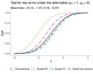
Figure 6: Average of conditional empirical CDFs of arm 1 from repeated sequential tests for two arms under the alternative hypothesis ($\mu_{1}=1,\mu_{2}=0$). See Section 4.2 for the detailed explanation about the sequential test.

As we conducted in Section 4.2, we have two standard normal arms with means $\mu_{1}$ and $\mu_{2}$. Then, we use the following upper and lower stopping boundaries to test whether $\mu_{1}\leq\mu_{2}$ or not:

$$U(t):=z_{\alpha/2}\sqrt{\frac{2}{t}},\quad\text{and}\quad L(t)=-U(t),$$ (63)

where $\alpha$ is set to $0.2$ to show the bias better. In contrast to the experiment in Section 4.2 in which the true means are equal to each other, in this experiment, we set $\mu_{1}=1$ and $\mu_{2}=0$ to make the alternative hypothesis is true.

Figure 6 show the marginal and conditional biases of the empirical CDFs and sample means for arm $1$ based on $10^{5}$ repetitions of the experiment. The black solid line corresponds to the true underlying CDF. The red dashed line refers to the average of the marginal CDFs, and the purple long-dashed line corresponds to the average of the empirical CDFs conditionally on reaching the maximal time. For these two cases, although the marginal CDF is negatively and the conditional CDF is positively biased, these are not general phenomena and the sign of bias can be changed as we change mean parameters.

However, for the cases corresponding to accepting $H_{1}$ (blue dot-dashed line) and accepting $H_{0}$ (green dotted line), we can check that signs of biases of CDFs and sample means are consistent with what Theorem 2 and corresponding inequalities (18) to (17) described. Also note that the bias results do not depend on whether the arms are under the null or alternative hypotheses.

B.2 Experiment About the Bias of the Sequential Halving Algorithm in Section 4.4

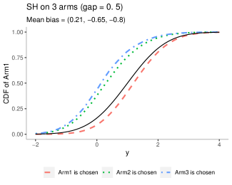
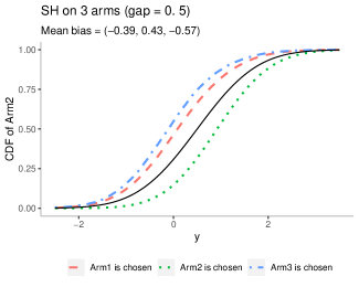
Figure 7: Average of conditional empirical CDFs of arm 1 (left) and arm 2 (right) from $10^{5}$ the sequential halving algorithm runs on three unit-variance normal arms with $\mu_{1}=1,\mu_{2}=0.5$ and $\mu_{3}=0$, as described in Section B.2. Black solid lines refer to the true CDF of arm 1 and arm 2.

To verify the conditional bias results in Corollary 7 and 8, we conducted $10^{5}$ trials of the sequential halving algorithm on three unit-variance normal arms with $\mu_{1}=1,\mu_{2}=0.5$ and $\mu_{3}=0$ as we did for the lil’UCB algorithm in Section 4.3. Again, it is important to note that the signs of the biases do not depend on the choice of parameters or of the underlying distributions, but the magnitudes of the biases do. To best illustrates the bias results, we use an unusually small time budget $T=10$ in this experiment.

The left side of Figure 7 shows the averages of the empirical CDFs of arm 1 (the arm with the largest mean) conditionally on each arm being chosen as the best arm. The thick black line corresponds to the true underlying CDF. The red dashed line, which lies below the true CDF, indicates that the empirical CDF of arm 1 conditionally on the event that arm 1 is chosen as the best arm (i.e., $\kappa=1$) is negatively biased; this then implies that the sample mean of the chosen arm is positively biased. In contrast, the green dotted and blue dot-dashed lines, lying above the true CDF, show that conditionally on the event that arm 1 is not chosen as the best arm (i.e., $\kappa\neq 1$), the empirical CDF is positively biased and the sample mean is negatively biased.

The right side of Figure 7 displays the averages of the empirical CDFs of arm 2. Though arm 2 is not the best arm, we can check that the signs of the conditional biases follow the same pattern as arm 1. Conditionally on the event that arm 2 is chosen as the best arm ($\kappa=2$), the empirical CDF is negatively biased (green dotted line), but conditionally on the event that arm 2 is not chosen as the best arm ($\kappa\neq 2)$, the corresponding CDFs are now positively biased (red dashed and blue dot-dashed lines), as expected.

B.3 Experiments on Conditional Biases of Sample Variance and Median in MABs

As stated in Section 5, characterizing the bias of other important functionals such as sample variance and sample quantiles is an important open problem. In this subsection, we present a simulation study on the bias of sample variance and median.

For a given $n\geq 2$ i.i.d. samples $X_{1},\dots,X_{n}$ from a distribution $P$, the sample variance $\widehat{\sigma}^{2}$ and median $\widehat{m}$ are defined by

$$\widehat{\sigma}^{2} =\frac{1}{n-1}\sum_{i=1}^{n}(X_{i}-\bar{X}_{n})^{2}$$ (64)

$$\widehat{m} =\begin{cases}\frac{1}{2}\left(X_{(n/2)}+X_{(n/2+1)}\right)&\mbox{if $n$ is even},\\ X_{(\frac{n+1}{2})}&\mbox{if $n$ is odd},\end{cases}$$ (65)

where $\bar{X}_{n}$ corresponds to the sample mean and $X_{(i)}$ refers to the $i$-th smallest sample.

It is well-known that for any distribution $P$ with finite variance $\sigma^{2}$, the sample variance $\widehat{\sigma}^{2}$ is an unbiased estimator of $\sigma^{2}$. Also, though the sample median is not necessarily unbiased, for any symmetric distribution $P$ including the normal distribution as a special case, the sample median is unbiased. However, for adaptively collected data from a MAB experiment, it is unclear whether the sample variance and median are unbiased or not. Furthermore, it is an open question how to characterize the bias of sample variance and median estimators if they are biased estimators.

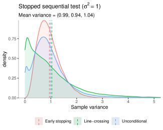
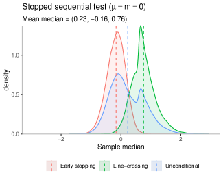
Figure 8: Left: Densities of observed sample variances from repeated stopped sequential test as described in Section 4.1. Right: Densities of observed sample median from the same repeated stopped sequential test. For both figures, vertical dashed lines correspond to averages of sample variances and medians on each conditions.

As an initial step, we conduct the repeated sequential experiments described in Section 4.1 and empirically investigate the biases of the sample variance and median estimators. Figure 8 describes a simulation study on the bias of the sample variance in the sequential testing setting of Section 4.1. Recall that, in this experiment, we have a stream of samples from a standard normal distribution. Each test terminates once either the number of samples reaches a fixed early stopping time $M=10$ or the sample mean crosses the upper boundary $t\mapsto\frac{z_{\alpha}}{\sqrt{t}}$ with $\alpha=0.2$.

Figure 8 shows the marginal and conditional distributions of the sample variance and median from $10^{5}$ stopped sequential tests. Vertical lines correspond to averages of the sample variances and medians over repetitions of the experiment and under different conditions. For the sample variance, the simulation shows that the sample variance is negatively biased marginally and conditionally on the early stopping event. On the other hand, conditionally on the line-crossing event, the sample variance has a heavy right tail and is positively biased. For the sample median, we can check that, marginally and conditionally on the line-crossing event, the sample median is positively biased. In contrast, the sample median is negatively biased conditionally on the early stopping event. Note that, for the sample median, sizes of biases of the sample median are similar to ones from the sample means which were equal to $(0.22,-0.16,0.75)$.

References

- Agrawal & Goyal (2012) Agrawal, S. and Goyal, N. Analysis of thompson sampling for the multi-armed bandit problem. In Conference on Learning Theory, pp. 39–1, 2012.
- Audibert & Bubeck (2009) Audibert, J.-Y. and Bubeck, S. Minimax policies for adversarial and stochastic bandits. In COLT, pp. 217–226, 2009.
- Auer et al. (2002) Auer, P., Cesa-Bianchi, N., and Fischer, P. Finite-time analysis of the multiarmed bandit problem. Machine learning, 47(2-3):235–256, 2002.
- Bowden & Trippa (2017) Bowden, J. and Trippa, L. Unbiased estimation for response adaptive clinical trials. Statistical methods in medical research, 26(5):2376–2388, 2017.
- Deshpande et al. (2018) Deshpande, Y., Mackey, L., Syrgkanis, V., and Taddy, M. Accurate inference for adaptive linear models. In Proceedings of the 35th International Conference on Machine Learning, 2018.
- Even-Dar et al. (2002) Even-Dar, E., Mannor, S., and Mansour, Y. Pac bounds for multi-armed bandit and markov decision processes. In International Conference on Computational Learning Theory, pp. 255–270. Springer, 2002.
- Even-Dar et al. (2006) Even-Dar, E., Mannor, S., and Mansour, Y. Action elimination and stopping conditions for the multi-armed bandit and reinforcement learning problems. Journal of machine learning research, 7(Jun):1079–1105, 2006.
- Garivier & Cappé (2011) Garivier, A. and Cappé, O. The KL-UCB algorithm for bounded stochastic bandits and beyond. In Proceedings of the 24th Annual Conference On Learning Theory, pp. 359–376, 2011.
- Gut (2009) Gut, A. Stopped random walks. Springer, 2009.
- Hadad et al. (2019) Hadad, V., Hirshberg, D. A., Zhan, R., Wager, S., and Athey, S. Confidence intervals for policy evaluation in adaptive experiments. arXiv preprint arXiv:1911.02768, 2019.
- Jamieson et al. (2014) Jamieson, K., Malloy, M., Nowak, R., and Bubeck, S. lil’ UCB: An Optimal Exploration Algorithm for Multi-Armed Bandits. In Proceedings of The 27th Conference on Learning Theory, volume 35 of Proceedings of Machine Learning Research, pp. 423–439, 2014.
- Kalyanakrishnan et al. (2012) Kalyanakrishnan, S., Tewari, A., Auer, P., and Stone, P. Pac subset selection in stochastic multi-armed bandits. In ICML, volume 12, pp. 655–662, 2012.
- Karnin et al. (2013) Karnin, Z., Koren, T., and Somekh, O. Almost optimal exploration in multi-armed bandits. In International Conference on Machine Learning, pp. 1238–1246, 2013.
- Kaufmann et al. (2012) Kaufmann, E., Korda, N., and Munos, R. Thompson sampling: An asymptotically optimal finite-time analysis. In International Conference on Algorithmic Learning Theory, pp. 199–213. Springer, 2012.
- Lattimore & Szepesvári (2019) Lattimore, T. and Szepesvári, C. Bandit algorithms. Cambridge University Press, 2019.
- Neel & Roth (2018) Neel, S. and Roth, A. Mitigating bias in adaptive data gathering via differential privacy. In International Conference on Machine Learning, pp. 3717–3726, 2018.
- Nie et al. (2018) Nie, X., Tian, X., Taylor, J., and Zou, J. Why adaptively collected data have negative bias and how to correct for it. In International Conference on Artificial Intelligence and Statistics, pp. 1261–1269, 2018.
- Paulson et al. (1964) Paulson, E. et al. A sequential procedure for selecting the population with the largest mean from normal populations. The Annals of Mathematical Statistics, 35(1):174–180, 1964.
- Robbins (1952) Robbins, H. Some aspects of the sequential design of experiments. Bulletin of the American Mathematical Society, 58(5):527–535, 1952.
- Shin et al. (2019a) Shin, J., Ramdas, A., and Rinaldo, A. Are sample means in multi-armed bandits positively or negatively biased? In Advances in Neural Information Processing Systems, pp. 7100–7109, 2019a.
- Shin et al. (2019b) Shin, J., Ramdas, A., and Rinaldo, A. On the bias, risk and consistency of sample means in multi-armed bandits. arXiv preprint arXiv:1902.00746, 2019b.
- Starr & Woodroofe (1968) Starr, N. and Woodroofe, M. B. Remarks on a stopping time. Proceedings of the National Academy of Sciences of the United States of America, 61(4):1215, 1968.
- Sutton & Barto (1998) Sutton, R. S. and Barto, A. G. Introduction to reinforcement learning. MIT press Cambridge, 1998.
- Thompson (1933) Thompson, W. R. On the likelihood that one unknown probability exceeds another in view of the evidence of two samples. Biometrika, 25(3/4):285–294, 1933.
- Villar et al. (2015) Villar, S. S., Bowden, J., and Wason, J. Multi-armed bandit models for the optimal design of clinical trials: benefits and challenges. Statistical science: a review journal of the Institute of Mathematical Statistics, 30(2):199, 2015.
- Xu et al. (2013) Xu, M., Qin, T., and Liu, T.-Y. Estimation bias in multi-armed bandit algorithms for search advertising. In Advances in Neural Information Processing Systems, pp. 2400–2408, 2013.