APOGEE Net: Improving the derived spectral parameters for young stars through deep learning

Abstract

Machine learning allows efficient extraction of physical properties from stellar spectra that have been obtained by large surveys. The viability of ML approaches has been demonstrated for spectra covering a variety of wavelengths and spectral resolutions, but most often for main sequence or evolved stars, where reliable synthetic spectra provide labels and data for training. Spectral models of young stellar objects (YSOs) and low mass main sequence (MS) stars are less well-matched to their empirical counterparts, however, posing barriers to previous approaches to classify spectra of such stars. In this work we generate labels for YSOs and low mass MS stars through their photometry. We then use these labels to train a deep convolutional neural network to predict $\log g$, $T_{eff}$ and Fe/H for stars with APOGEE spectra in the DR14 dataset. This “APOGEE Net” has produced reliable predictions of $\log g$ for YSOs, with uncertainties of within 0.1 dex and a good agreement with the structure indicated by pre-main sequence evolutionary tracks, . These values will be useful for studying pre-main sequence stellar populations to accurately diagnose membership and ages.

1 Introduction

Spectroscopy is a powerful technique for measuring stellar properties, and in recent years, large surveys such as SDSS APOGEE (Abolfathi et al., 2018), RAVE (Kunder et al., 2017), and GALAH (Buder et al., 2018) have observed 10^5-6 stars each. This necessitates an effective method to uniformly and efficiently process these spectra to extract the stellar properties (e.g., effective temperature ($T_{eff}$), surface gravity ($\log g$), and metallicity (Fe/H).

A common approach to spectral analysis rely on comparisons between the target spectrum and a grid of spectral standards (that may be difficult to come by for specific source types or wavelength range) or synthetic templates (that may systematically differ from the real data). Synthetic templates typically offer more regular coverage of parameter space, enabling individual targets’ parameters to be inferred precisely by using a higher order function to interpolate the goodness of fit parameters between the points for which the grid is defined. Many surveys adopt this approach in constructing their stellar parameter pipelines (e.g., García Pérez et al., 2016), but the process is computationally intensive, particularly when fitting multiple parameters simultaneously, as well as determining the corresponding uncertainties.

Computational efficiency aside, the reliability of parameters determined via direct model fitting can also vary strongly as a function of target type, with young stellar objects (YSOs) representing a particularly challenging target class (e.g., Doppmann et al., 2005). Spectral fits can return reasonably accurate estimates of $T_{eff}$ for YSOs, but $\log g$ has proven more difficult to accurately constrain. This parameter is particularly valuable for YSOs, as it serves as a proxy for stellar age, and is therefore of great value for calibrating pre-main sequence evolutionary models or inferring star formation histories within a given star forming complex. The APOGEE survey has conducted extensive surveys of several nearby star forming regions, providing a valuable opportunity to infer $\log g$ and age constraints for large samples of YSOs, but those constraints have been difficult to achieve in practice. For APOGEE data in particular, obtaining reliable $\log g$ values for dwarf or pre-main sequence stars have been challenging: neither APOGEE’s primary stellar parameter pipeline, ASPCAP (Holtzman et al., 2015; García Pérez et al., 2016), nor the community-provided Payne model-fitting framework (Ting et al., 2019) released $\log g$ estimates for dwarf stars, due to the presence of clear systematic errors in uncalibrated values and the lack of a densely sample comparison sample for deriving calibration relations. The IN-SYNC pipeline (Cottaar et al., 2014; Kounkel et al., 2018), developed and optimized for YSO spectra, provided $\log g$ values whose age dependence agrees well with physical models , but the precise values also show unphysical systematics, likely due to mismatches between the empirical and theoretical spectra.

Data driven analysis pipelines eliminate errors due to model mismatches, by training prediction systems with empirical spectra for stars with well determined stellar parameters. One data-driven method that has demonstrated considerable success in assigning labels to APOGEE spectra is The Cannon (Ness et al., 2015), which uses a reference sample of APOGEE spectra to train a that can then be used to infer stellar parameters for any object with an APOGEE spectrum. Using the full wavelength information within the spectrum, and training on empirical standards that eliminate the potential for model-data mis-fitting, the Cannon is able to provide parameters of comparable quality to ASPCAP’s for APOGEE spectra with SNR $\geq$ 25. As informed by a set of 60 dwarf calibrators in the Hyades, the 2015 Cannon results also included realistic $\log g$ values for the upper main sequence, but became incomplete for dwarfs with T${}_{eff}<$ 4500 K, similar to the limit reached by the Payne results. While data driven models offer important performance and calibration advantages, they are unable to overcome the limits of their training sets.

Neural networks offer a promising data driven method for inferring accurate stellar parameters from spectra, and with a potentially greater flexibility in inference methods than offered by the polynomial formalism adopted in the Cannon. Neural networks are a common machine learning model, in which multiple non-linear transformations of the input features are performed before assigning an output classification. A number of studies have demonstrated the ability of neural networks to classify stellar spectra , e.g., Bailer-Jones et al. (1997); Bailer-Jones (2000); Bazarghan & Gupta (2008); Fabbro et al. (2018); Sharma et al. (2019); Leung & Bovy (2019). Neural networks also offer important efficiencies for processing large datasets. Direct fitting can only consider a single spectrum at a time, redoing the same operation regardless of how similar two target spectra may be. On the other hand, neural networks can process in excess of $10^{6}$ observations in under an hour. As with all data-driven methods, however, the network must be trained on a reliable reference sample whose parameters span the full range of interest, making the construction of a label-set as important as the construction of the network itself.

In this paper we aim to train a deep neural network to accurately classify APOGEE DR14 spectra of dwarfs, giants, and pre-main sequence stars. To realize this goal, we first supplement the stellar labels provided by the Payne with a set of labels inferred from Gaia, 2MASS and Pan-STARRS photometry and astrometry for YSOs and M dwarfs with APOGEE spectra. In Section 2 we describe the data and the procedure used to generate the labels. In Section 3 we then construct a convolutional neural network (CNN) that predicts parameters from the APOGEE spectra, which we refer to as the APOGEE Net. In Section 4 we highlight some analysis that could be derived from these spectral properties. Finally, we summarize our results and discuss the implications in Section 5.

2 Data

2.1 APOGEE

Apache Point Observatory Galactic Evolution Experiment (APOGEE) is a high resolution (R$\sim$22,500) near infrared (1.511.7 $\mu$m spectrograph mounted on a Sloan Foundation 2.5m telescope (Gunn et al., 2006; Wilson et al., 2010; Blanton et al., 2017; Majewski et al., 2017). APOGEE is capable of observing up to 300 targets in a field of view 1.5^∘. Over the years, the survey and its targeting priorities has evolved. The primary objective of both APOGEE-1 and APOGEE-2 has been to observe red giants to trace the dynamical and the chemical patterns of the Galaxy (e.g., Hayden et al., 2015; Bovy et al., 2016; Anders et al., 2017; Zasowski et al., 2017). However, it has also observed a number of star-forming regions, including Orion Complex (Da Rio et al., 2016, 2017; Kounkel et al., 2018), NGC 1333 (Foster et al., 2015), IC 348 (Cottaar et al., 2015), NGC 2264, as well as several more evolved clusters, and some of the nearby main sequence stars.

As of the public Data Release 14 (Abolfathi et al., 2018), over 263,000 stars in the bulge, disk, and halo have been observed. We restrict the current analysis only to these sources.

The sources in the catalog typically have been observed for multiple epochs. Therefore, the data are stored in two formats: ‘apVisit’, which contains the raw spectrum at a particular epoch, and ‘apStar’, in which the Doppler shift has been removed from the epochs, placing them all in a common rest frame with identical wavelength solution across all sources, and multiple visits for the same source are combined into one, increasing the resulting signal-to-noise (Nidever et al., 2015).

2.2 Payne Labels

Ting et al. (2019) used their newly developed spectral interpolator, along with a new grid of Kurucz spectral models calculated with an improved line list (Cargile et al., 2019), to identify best-fit models & infer revised stellar parameters for 222,707 spectra within the APOGEE DR14 dataset. The labels inferred from this interpolator, dubbed ‘The Payne’ in honor of Cecilia Payne-Gaposchkin’s seminal work in physically-based stellar models, are comparable to the calibrated parameters provided in DR14 for stars along the Red Giant Branch. Moreover, the Payne provides realistic $T_{eff}$ and $\log g$ labels for warmer ($T_{eff}$$>4250$ K) main sequence stars, for which calibrated parameters are not available in the DR14 dataset. Typical uncertainties, both random and systematic, are $\sim$100 K in T_eff, $\sim$0.1 dex in $\log g$, and $\sim$0.03 dex in abundance space (Ting et al., 2019).

However, the Payne has non-physical correlations between $\log g$ and Fe/H towards cooler dwarfs. Indeed, these systematics dominated the information content of the Payne labels to such a degree that dwarfs stars with $T_{eff}$$<$ 4000 K were intentionally removed from the Payne outputs, to avoid potential mis-interpretation of the spurious correlation between the inferred log g and [Fe/H] values.

In training APOGEE Net, we adopt labels from the Payne’s outputs for stars with $T_{eff}$$>$ 4000 K or $\log g$$<$ 3.5 we to generate new labels for 4,480 low mass main sequence stars and 2446 YSOs .

2.3 Deriving Alternate Labels for pre-main sequence & low mass main sequence stars

2.3.1 MS stars

We begin by identifying bona fide lower main sequence stars with potentially erroneous Payne labels, using 2MASS & Gaia DR2 photometry, as well as Gaia’s parallax measurements. We selected low mass MS stars by requiring 2MASS photometry of 0.7$<J-K<$1.05, 3.37$<g-K<$8.46, and 5$<M_{K}<$10. To ensure accurate $M_{K}$, we further restricted the sample to only those sources in which the Gaia DR2 measured $\pi/\sigma_{\pi}>3$; this removed any giants with erroneous M_K values due to spurious, low-quality parallaxes. Since the empirical relations used in this section were calibrated for main sequence stars, we flag all spectra within APOGEE fields covering known star-forming regions and young clusters – namely the Orion Complex, Perseus clusters, NGC 2264, and the Pleiades – for a separate label generation procedure, which is described in the next section.

We infer metallicities for these stars using the relation by Hejazi et al. (2015)

$$[Fe/H]=A_{1}+A_{2}(g-K)+A_{3}(J-K)+A_{4}(g-K)^{2}+\\ A_{5}(J-K)^{2}+A_{6}(g-K)(J-K)$$ (1)

in which

$$A=[-14.259,0.0519,29.5926,$$

$$-0.0529,-17.6762,0.7032]$$

This calibration is applicable for stars between K6 and M6.5, with $-0.73\leq[Fe/H]\leq+0.3$ dex, $3.3\leq g-K\leq 8.46$ and $0.71\leq J-K\leq 1.01$. By design, these limits nearly exactly match the color-mag cuts used to select candidates for our alternate, pre-main sequence focused label generation procedure. We do allow a modestly broader range of $g-K$ colors, by a few hundredths of a magnitude in each direction, as the extrapolated metallicities will nontheless likely be more accurate than the Payne parameters, which clearly suffer from systematic errors in this space.

To estimate $T_{eff}$, we use the relation from Mann et al. (2015)

$$T_{eff}=B_{0}+B_{1}(r-J)+B_{2}(r-J)^{2}+B_{3}(r-J)^{3}+\\ B_{4}(r-J)^{4}+B_{5}(J-H)+B_{6}(J-H)^{2}$$ (2)

with

$$B=[2.151,-1.092,0.3767,-0.06292,$$

$$0.003950,0.1697,-0.03106]$$

which hold for $4.6<M_{K}<9.8$, 2700$<$$T_{eff}$$<$4100 K, and -0.6 $<$[Fe/H]$<$ 0.5.

Finally, to estimate $\log g$  we use the relation from Veyette et al. (2017)

$$\log g=7.912-0.1880\times[Fe/H]-1.334\times 10^{-3}\times T_{eff}+\\ 1.313\times 10^{-7}\times T_{eff}^{2}$$ (3)

which hold for 3200$<$$T_{eff}$$<$4100 K and -0.7 $<$ [Fe/H] $<$ 0.3.

2.4 YSOs

Figure 1:

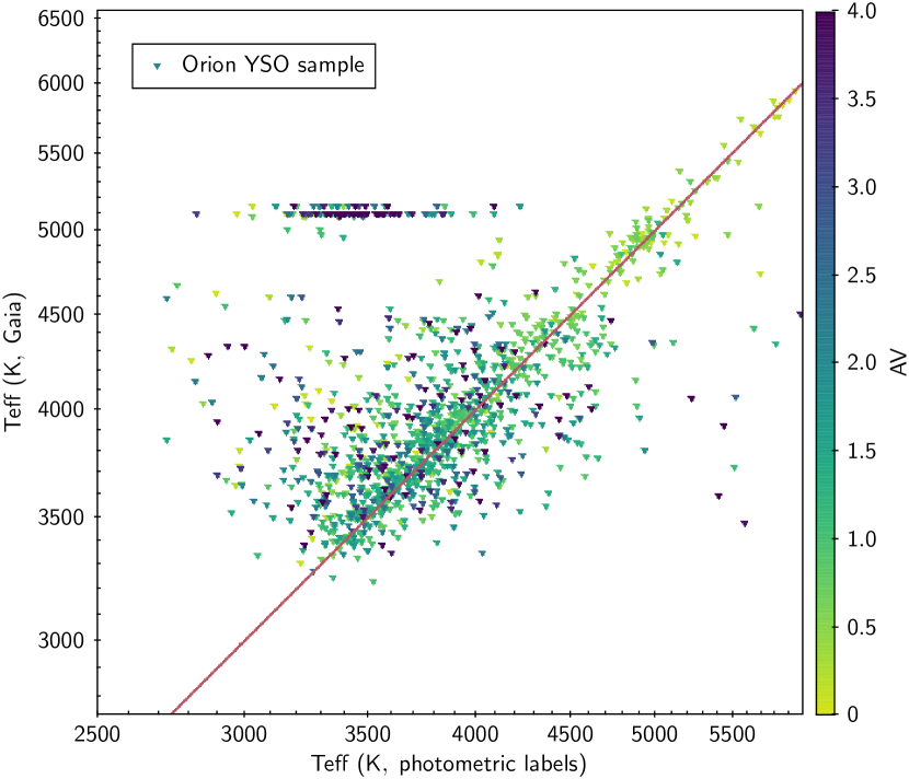
Figure 2: Comparison of the $T_{eff}$ derived from the photometric CNN versus $T_{eff}$ from Gaia Collaboration et al. (2018) for the YSOs.

The APOGEE fields designed to target star-forming regions nonetheless include sources other than YSOs. To calculate parameters for a pure YSO sample, we restricted the sample to likely cluster members tabulated by Kounkel et al. (2019), with spectra publicly released in DR14 (Abolfathi et al., 2018).

We attempted multiple approaches to interpolate each YSO’s photometry onto a grid of isochrones to $T_{eff}$ and $\log g$ . We considered various isochrones for this purpose, including those from Baraffe et al. (2015), PARSEC (Marigo et al., 2017), and MIST (Choi et al., 2016). We assessed combinations of various photometric bands from 2MASS, WISE, and Gaia, and explored the ability to assign reliable stellar labels using standard isochrone fits (as implemented via the ’isochrones’ python package, developed by Timothy Morton).

As an alternative , we constructed a CNN with three convolutional layers using max pooling and two fully connected layers. This network was trained on parameters from synthetic stars drawn from the PARSEC isochrones . The synthetic stars were generated using a uniform distribution of stellar masses from 0.08 to 3 M_⊙, ages from 1 to 100 Myr, extinction from 0 to 20 $A_{V}$, and distance from 50 to 1000 pc. Fe/H =0 were used, which is consistent with the nearby star-forming regions (e.g., D’Orazi et al., 2009, 2011). The empirical parameters the network used to evaluate the labels included 9 photometric bands, stellar radii $r_{*}$, stellar luminosities $\log L$, and the distance. In cases where the photometry in a particular band was too faint to be reliably detected in the real data, it was set to the limiting magnitude ($G<19$, $G_{BP}<20.5$, $G_{RP}<17.5$, $J<17$, $H<16$, $K<16$, $W1<16$, $W2<16$, $W3<13.5$), with only $G$ band being required. The additional two parameters $r_{*}$ and $\log L$, were drawn from the isochrone but modeled after those reported by Gaia DR2, in that they were only reported if $r_{*}>0.5r_{\odot}$, $\log L$$>-1.54$, and $M_{G}<10$. Similarly with the photometric bands they were set to the limiting cases if they were not detectable. No scatter due to uncertainties was applied to the synthetic parameters.

The CNN was trained on $\sim$42,000 synthetic stars to predict ages, masses, $A_{V}$, $T_{eff}$, and $\log g$ based on these input parameters. Applied on a separate synthetic sample that was generated similarly to the one on which it has been trained, not accounting for any uncertainties or systematic offsets, the neural network could recover $\log g$ with a precision of 0.01 dex, and $\log$ $T_{eff}$ with a precision of 0.003 dex.

When applied to the real data, the CNN produced $\log g$ that are consistent with the isochrones corresponding to the typically accepted ages of the individual clusters covered by APOGEE (Section 4). Additionally, it could generally recover $T_{eff}$ estimated by Gaia DR2 (Figure 2).

3 APOGEE Net

The APOGEE Net was designed to take in the raw spectra, and to return the predictions on $T_{eff}$, $\log g$, and Fe/H. The sources, labels of which were determined in Section 2, were split into three different subsets: a training set on which the model is trained, a held out development set which is used to evaluate the model’s generalization performance during training and to tune hyperparameters, and finally a held out test set which is used to evaluate the model’s performance once it has completed training. For the Payne catalog, the split between the train, dev, and test sets was 80/10/10%. Due to a smaller number of sources in other categories, to have a sufficient number of sources in the test set, M dwarf and YSO catalogs were split 60-20-20%.

3.1 Feature and Target Preprocessing

While we experimented with using various lossless normalization techniques for the input flux (i.e., not altering the underlying shape of the spectrum, merely scaling it) these standardized fluxes failed to converge in training, and we found training on the raw flux from the ‘apStar’ readily converged to good results. We did not investigate the performance of the ‘apStar’ spectrum normalized in a way that removes the underlying shape of the SED, as, depending on the spectral type, such normalization may be uncertain and result in the additional noise in the line profile. The main benefit of the normalization would be removal of the extinction signature from the spectrum, however, it should be possible for a neural network to learn to ignore reddening from the raw flux as well. Nonetheless, comparison in the performance between normalized and raw spectra could be a fruitful avenue for further investigation.

In contrast, in order to predict $T_{eff}$, $\log g$, and Fe/H simultaneously, it was necessary to normalize these target values; normalizing the targets put the losses (and gradients during training) onto a comparable scale. To normalize, we calculated the mean ($\mu$) and standard deviation ($\sigma$) of each target variable using the training set and then standardized all prediction targets across all sources and all sets (train, development, and test). Specifically, we normalized as follows:

$$\frac{x_{i}-\mu_{x}}{\sigma_{x}},$$ (4)

where $x$ denotes a target variables ($T_{eff}$, $\log g$ or Fe/H) and $i$ denotes a specific datapoint. Normalization values can be found in Table 1.

For evaluation purposes, the model’s predictions are converted back to their physical units using the inverse relations from the above.

$\mu_{logg}$	2.88
$\sigma_{logg}$	1.16
$\mu_{Teff}$	4716.92
$\sigma_{Teff}$	733.01
$\mu_{Fe/H}$	-0.22
$\sigma_{Fe/H}$	0.30

Table 1: Normalization values for $T_{eff}$, $\log g$ and Fe/H

3.2 Convolutional Spectral Model

Our model is a one-dimensional CNN, inspired by the VGG16 CNN architecture (Simonyan & Zisserman, 2014). It consists of 12 convolutional layers separated every two layers by a max-pooling layer, followed by 2 fully connected layers (See Appendix A for term definitions and details). The model was implemented in PyTorch (Paszke et al., 2017). The architecture of the network is defined precisely in Appendix B.

3.3 Training and Tuning

We trained the APOGEE Net using stochastic gradient descent to minimize mean squared error (MSE) loss. To improve the model’s ability to generalize to new data, we employed early stopping; i.e., we stopped training when performance on the development set begins to decrease, which is indicative of overfitting to the training set at the expense of generalizability. After each full pass through the training data, the model’s performance is evaluated on the development set. If the development set performance has improved, as measured by a decrease in loss, then the model is saved. If, however, the loss on the development set does not improve after five consecutive evaluations, training is stopped. If the loss improves before the fifth evaluation, the model is saved, the counter resets and training resumes.

After a modest amount of hyperparameter tuning, we settled upon the following hyperparameter configuration: learning rate of 0.001, dropout rate of 0.1, and a training batch size of 128.

3.4 Model Adaptation

In order to obtain high model performance on our set of interest (YSOs and M-Stars), we explored various strategies for adapting a model trained on a larger set of data to our smaller set of YSOs and M-Stars. Another strategy was to first train on all stars, and then further train exclusively on the subset of interest. Unfortunately, this approach proved suboptimal: while the model performance did improve significantly for M-Stars and YSO stars, it resulted in a dramatic degradation in performance for the red giants in the Payne catalog.

Instead, After initially training APOGEE Net to convergence on the entire dataset, we continued training on the YSO and M-Star samples plus a random 5% of the Payne catalog. Each time the model stopped from early stopping, the last best performing model was be reloaded and another random 5% of the Payne catalog was selected to train on. Through this method, we were able to focus training on the M-Star and YSO data without losing performance on the broader Payne data set. This process continued until the performance on M dwarfs and YSOs did not show continuing improvement. Final normalized MSE loss performances for training, development and test after tuning are reported in Table 2, and the resulting performance for each parameters in the native units is shown it Table 3.

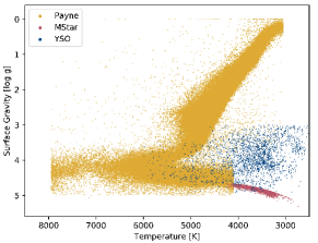
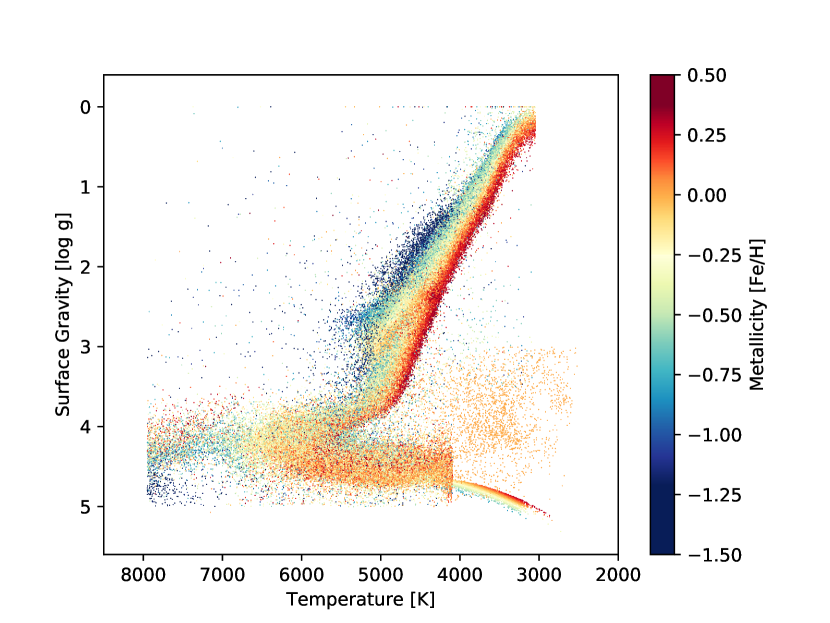
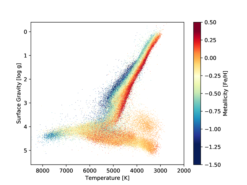
Figure 3: $T_{eff}$ and $\log g$ distribution of the sample. Top: Categorization of the input parameters based on the origin of the measurements. Middle: The input parameters used in training. Bottom: The resulting predictions from the APOGEE Net.

3.5 Uncertainties

Fundamentally, the predictions of a CNN are deterministic: after a model is trained, passing the same set of inputs always results in the same outputs. As is, the CNN is unable to realize the uncertainties in either the original data, or in its predictions (other than through a difference relative to the input labels).

However, given that the data themselves are uncertain, it is possible to vary inputs within the errors and retain the same underlying information. Each one of the realizations of the same spectrum would be perceived by the CNN as a distinct input, and would produce a slightly different prediction from the original. Measuring the scatter in these predictions can give an estimate of the uncertainties on the per source basis, akin to a Markov chain Monte Carlo. Although, unlike MCMC, this analysis is not particularly costly in terms of the computational time.

APOGEE has measured per pixel errors in flux. Therefore, at every pixel we generated a random value drawn from a normal distribution, multiplied it by the corresponding uncertainties, and added this noise profile to the flux. Some pixels (such as those near the chip gaps, or those that correspond to the telluric lines) had abnormally high uncertainties, to prevent them from skewing the model, we capped the maximum allowed error at 5 times the mean in the spectrum.

This procedure was repeated to generate 100 different realizations for each spectrum, and all of them were passed through the APOGEE Net. The mean and standard deviation values were then measured for each parameter for each source.

3.6 Validation of the stellar parameters

	MSE loss
	Train	Dev.	Test
Full	0.044	0.049	0.063
MStar	0.08	0.098	0.196
YSO	0.153	0.168	0.217

Table 2: Combined Standardized MSE loss

	Train	Dev.	Test
		Full
log g	0.189	0.203	0.216
Teff [K]	144.82	158.72	183.74
Fe/H	0.0769	0.0792	0.0914
		MStar
log g	0.186	0.216	0.346
Teff [K]	129.69	167.15	273.7
Fe/H	0.129	0.137	0.18
		YSO
log g	0.366	0.364	0.4
Teff [K]	413.92	436.87	490.99
Fe/H	0.0616	0.0669	0.0879

Table 3: The typical scatter between the input labels and the predictions for each parameter in each group

Figure 4: Left: Comparison between the input labels and the predicted spectroscopic parameters. Right: Uncertainties as a function of SNR.

We report on the resulting predictions with the corresponding uncertainties in Table 4.

The typical agreement between the input labels and the resulting predictions is 100 K in $T_{eff}$, 0.15 dex in $\log g$, and 0.07 dex in Fe/H (Table 3, Figure 4, left). The scatter in $T_{eff}$ and $\log g$ is slightly higher for the YSOs, as it improved on some of the systematic issues the photometric labels had, which were originally derived somewhat crudely, fine-tuning them based on the overall grid. For the M-stars, comparison between the labels and the predictions for Fe/H is slightly offset from the line of unity, with predictions somewhat compressing the range of Fe/H offered by the labels, having fewer sources as metal rich, and fewer as metal poor, but showing a good linear agreement overall.

The typical reported uncertainties are 25 K in $T_{eff}$, 0.04 dex in $\log g$, and 0.015 dex in Fe/H, thus they underestimate the scatter between the labels and the predictions by approximately a factor of 4. In comparison to other pipelines, the uncertainties for the same sources are not strongly correlated, but they are generally comparable to the errors reported by the IN-SYNC pipeline, and approximately a factor of 2 smaller than those reported by ASPCAP pipeline. The reported uncertainties strongly depend on the SNR of the spectrum, as well as on the spectral parameters (Figure 4, right). As expected, the parameters of hotter or more metal poor stars would be more uncertain due to a fewer number of lines that can be used to determine stellar properties. Similarly, sources with higher $\log g$ would have shallower lines, resulting in more uncertain predictions. Although the APOGEE Net had no information on the uncertainties in the labels, and the errors were generated from slightly perturbing the input spectral fluxes and taking an rms of the resulted predictions, it was able to reproduce physically expected trends.

At low SNR ($<$10—20), the uncertainties in all parameters reach a ceiling of $\sim$200 K in $T_{eff}$, $\sim$0.2 dex in $\log g$, and $\sim$0.1 dex in Fe/H. This ceiling suggests that the uncertainties for these sources are underestimated, furthermore, that the CNN does not derive any meaningful information in the low SNR spectra. This brings into question the reliability of other parameters (e.g., $v\sin i$, radial velocity) derived by other means in these low SNR spectra.

A similar approach to determining spectroscopic parameters from the APOGEE spectra for the M-dwarfs was recently undertaken by Birky et al. (2020), based on the Cannon (Ness et al., 2015) data-driven spectral modeling code (Figure 5). While some YSOs are included in their sample, they tend to have higher $\chi^{2}$ for the fit compared to the rest of the sample. In particular, because their code did not train to distinguish between metallicity and $\log g$, it considered YSOs to be more metal rich than they are likely to be due to deeper spectral lines. In the M-dwarf sample, for the metallicity, there is a good agreement at $Fe/H<0$, but at $Fe/H>0$ they tend to systematically differ by a factor of 2; it is not clear why. The predicted $T_{eff}$ appears to be comparable between the two works, with a scatter of $\sim$100 K. However, because they have not included any sources hotter than $\sim$4,100 K, they tend to run into the edge effects at $\sim$4,000 K, with sources piling at the boundary. We note that a similar effect occurs in this work as well, at $T_{eff}$$\sim$8,000 K – any stars intrinsically hotter than are interpolated towards this value. This potentially explains the excess of metal poor stars in Figure 3. For this reason we do not include any stars hotter than 6,700 K in Table 4. In future, however, by generating more reliable labels for massive stars and including them in the training, it would be possible to minimize these edge effects.

Figure 5: Left and center: Comparison of Fe/H and $T_{eff}$ derived in this work compared to those in Birky et al. (2020). The sources in the Valid sample satisfy the quoted ranges of the parameter space from Birky+ over which their extra extrapolation is applicable, combined with having uncertainties in the predicted parameters in our work of $\sigma_{T_{eff}}<$100 K and $\sigma_{\log\ g}<0.1$ dex (typically corresponding to SNR$>20$), restricting the comparison to 5893 stars. The YSO sample is a subset of the Valid sample, with the overlapping sources from Kounkel et al. (2019). Right: Comparison of the derived $T_{eff}$in this work and $T_{eff}$ from Gaia DR2. Note the edge effect at $T_{eff}$$\sim$4,000 K for the sample from Birky et al., and 8,000 K for the sample in this work.

4 Results

4.1 Overall properties

Table 4: Results for combined evaluation

APOGEE ID	$\alpha$	$\delta$	$\log g$	$\log g$	$\sigma$ $\log g$	$T_{eff}$	$T_{eff}$	$\sigma$ $T_{eff}$	Fe/H	Fe/H	$\sigma$ Fe/H	SNR	Data	Data
	(J2000)	(J2000)	(label, dex)	(prediction, dex)	(dex)	(label, K)	(prediction, K)	(K)	(label, dex)	(prediction, dex)	(dex)		Set	Type
2M00003379+7940362	0.140803	79.676727	4.94	4.47	0.06	3307	3357	28		-0.05	0.01	137.0	train	Mstar
2M00013219+0016012	0.384140	0.267008	4.74	4.64	0.08	3997	3998	47		-0.25	0.02	57.2	train	Mstar
2M00024474+6158060	0.686431	61.968346	4.74	4.50	0.10	3787	4062	50		-0.15	0.02	57.7	train	Mstar
2M00025988+0148410	0.749506	1.811404	4.72	4.65	0.07	3959	3919	32		-0.19	0.02	82.1	train	Mstar
2M00030930+0110025	0.788757	1.167374	4.73	4.66	0.07	3947	3974	33		-0.24	0.02	88.1	train	Mstar

Figure 6: Distribution of $T_{eff}$ and $\log g$ values for the YSOs across the various regions. The compilation of the measurements from the IN-SYNC pipeline (top), photometrically derived input labels (middle), and the resulting output from the APOGEE Net (bottom) are shown. The grey lines show the isochrones at ages of 1, 2, 5, 10, 20, 50, 100, 200, and 300 Myr, and 8.5 dex, as well as the evolutionary tracks for 0.4, 0.5, 0.6, 0.7, 0.8, 0.9, and 1 M_⊙ stars from the PARSEC isochrones (Marigo et al., 2017).

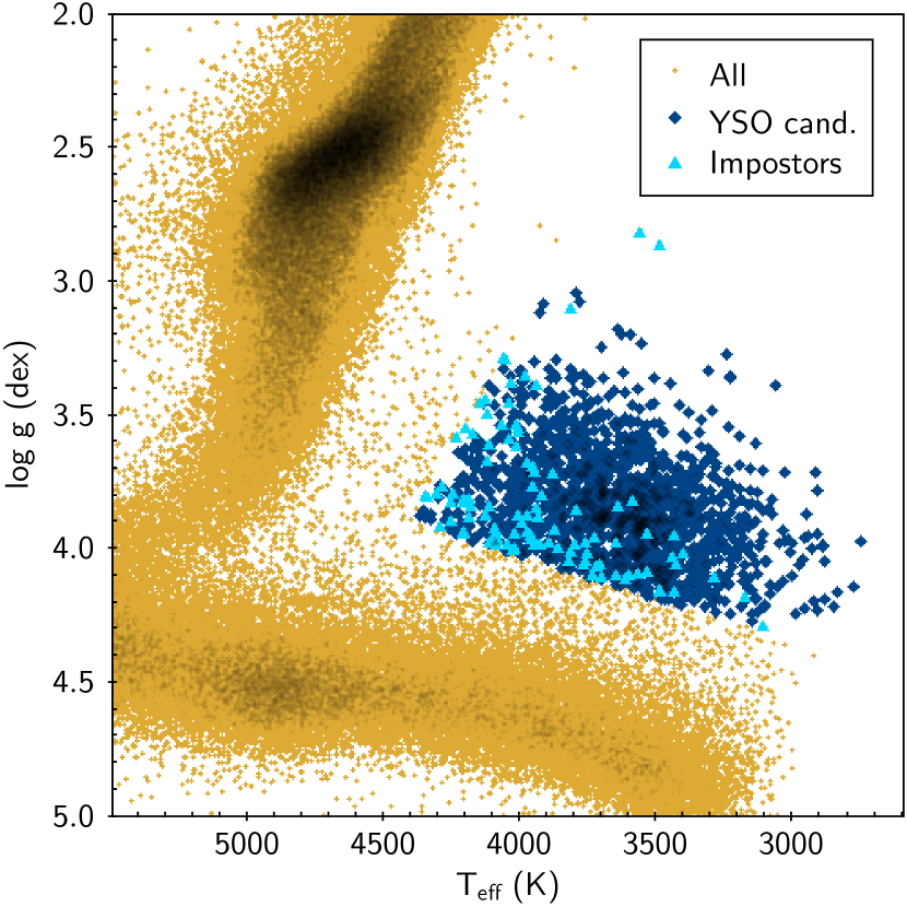
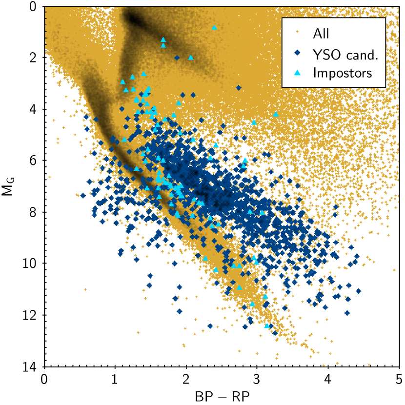
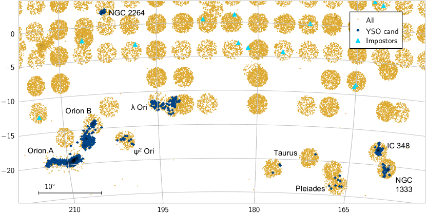
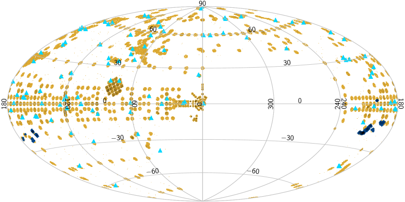
Figure 7: Top: Selection of the YSOs based on the predicted stellar parameters. Objects are considered YSO candidates if they fall into the parameter space bounded by ($T_{eff}$, $\log g$) of (2200,4.4) (4500,3.9), and (3200,1.7). Left panel shows the spectroscopic parameters, right panel shows the HR diagram constructed using Gaia photometry . Bottom: spatial distribution of the identified candidates in galactic coordinates. Sources that do not coincide with nearby star-forming regions are flagged as the potential impostors (6% of the sources in the selected area).

As can be seen in Figure 6, the quality of the derived $T_{eff}$ and $\log g$ for YSOs improves with each method for extracting them. The original parameters from the IN-SYNC pipeline are systematically offset from the isochrones, have an odd shape of the main sequence, and have various unphysical gaps, most notable of which is at $T_{eff}$=3,600 K. The labels derived from the photometry show similar agreement to the isochrones in the sequences of the ages of the individual regions, and it renormalizes the derived parameters to the appropriate range, but it does show a somewhat peculiar behavior especially at low $T_{eff}$ as it attempts to reconcile the differences between various bands and the isochrones.

Finally the APOGEE Net connects the derived parameters for the YSOs to those for the M dwarfs and the red giants, making it possible to interpret the resulting values, and removing all of the systematic gaps that persisted in the previous iterations. However, there may still be a weak systematic offset in the shape of the isochrones and the YSOs at $T_{eff}$$<3500$ K, as at a particular age, the isochrone tends result in somewhat lower $\log g$ at lower $T_{eff}$. On the other hand, $\log g$ traced by the individual stellar populations either remain flat throughout or slightly increase towards higher values at low $T_{eff}$, oriented in parallel to the main sequence. Considering that the photometric labels showed the opposite trend at lower $T_{eff}$, it is unclear how such a potential discrepancy could be better rectified in the future, or if the cause of the discrepancy is necessarily in the predicted parameters as opposed to the isochrones.

The spectroscopic parameter space that the low mass YSOs occupy can be rather cleanly separated from the other stellar objects, as they have $\log g$ typically lower than the main sequence stars, and $T_{eff}$ typically cooler than the red giants. Thus, by selecting the sources in this parameter space, we can robustly identify young stars in the catalog and look at their spatial distribution (Figure 7). With a simple cut, restricting the selection bound by ($T_{eff}$, $\log g$) of (2200,4.4) (4500,3.9), and (3200,1.7) it is possible to recover all of the star forming regions in the sample: the Orion Complex, Perseus clusters NGC 1333 and IC348, as well as NGC 2264. Some of the sources from Pleiades end up in this selection as well. Surprisingly, some fields (K2_C4_172-20 and K2_C4_177-21) also appear to include sources from the Taurus Molecular Clouds. While Taurus has been observed with APOGEE, the dedicated observations of young stars in this region have not begun until after the release of DR14. Thus, the sources we see have been observed serendipitously.

The aforementioned selection does not recover all of the young stars that have been observed, particularly those that are hotter or those that are somewhat more evolved. Additionally, approximately 6% of the sources from this simple selection are scattered all across the sky, many at high galactic latitudes, which do not appear to be associated with any particular star forming region, suggesting that they are impostors, i.e, contamination.

The distribution of the selected sources in the spectroscopic space is comparable to the distribution of sources in the HR diagram. Even the impostors appear to be bona fide sub-giants . Furthermore, this comparison demonstrates that it is possible to use the spectoscopically derived parameters to effectively derive stellar properties, even for sources that are located in regions of high extinction, those have very uncertain parallaxes, or no parallax measurements at all.

4.2 Ages

It is possible to use the derived $\log g$ values as a proxy for age. We have not explicitly interpolated the $T_{eff}$ and $\log g$ across the isochrones, however we divided the sample into 5 bins: $\log g$$<3.6$ dex ($\lesssim$1 Myr), $3.6<$$\log g$$<3.8$ dex (1$\sim$2 Myr), $3.8<$$\log g$$<4.0$ dex (2$\sim$3 Myr), $4.0<$$\log g$$<4.2$ dex (3$\sim$5 Myr), and $4.2<$$\log g$ dex ($\gtrsim$5 Myr). We then constructed a density map of sources in each bin (Figure 8). .

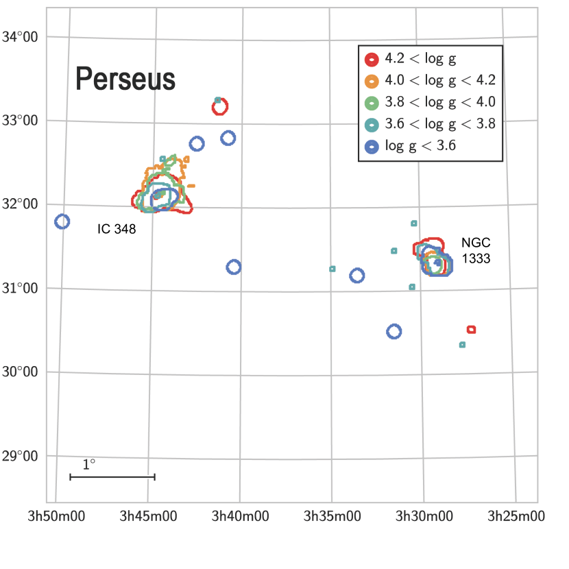
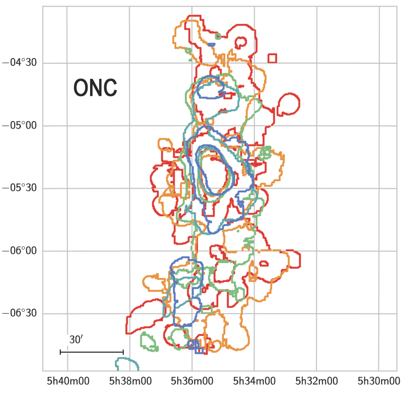
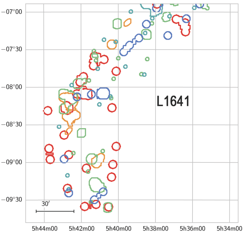
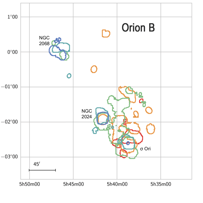
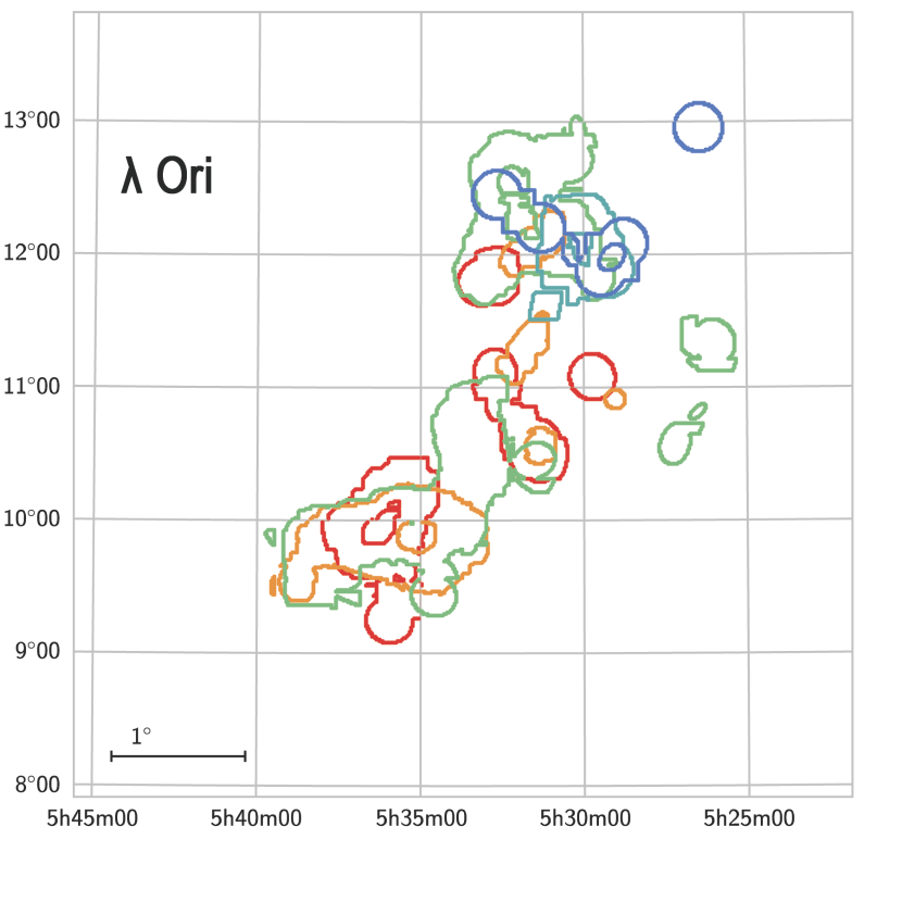
Figure 8: Contour plots showing the density distribution of sources with different $\log g$ values, as a proxy for age, color-coded from the youngest ($\lesssim$1 Myr, blue), to the oldest ($\gtrsim$5 Myr, red)

In Orion, the distribution of ages is largely consistent what has been previously measured for each individual region. For example, in $\lambda$ Ori, the central cluster is $\sim$5 Myr, and the outer shell that has been triggered by a supernova, consistent with what has been previously measured by Kounkel et al. (2018). In the vicinity Orion B, there is a clear separation between $\sim$1 Myr old clusters, NGC 2068 and NGC 2024, a somewhat older (2–3 Myr) cluster $\sigma$ Ori, and 3–5 Myr extended population associated with it. A similar agreement with previously measured ages can also be observed in $\psi^{2}$ Ori.

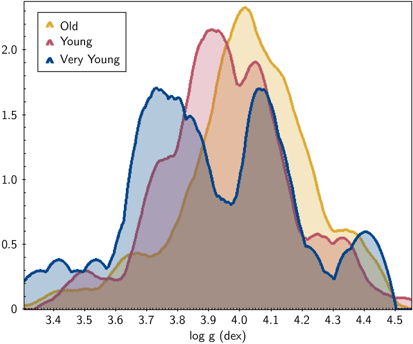
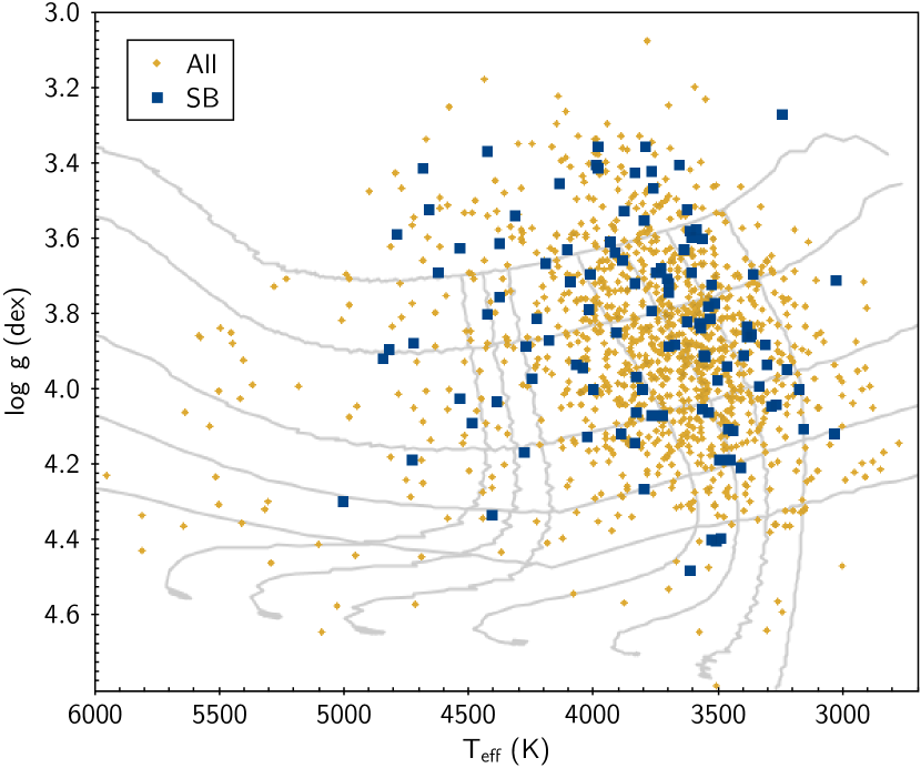
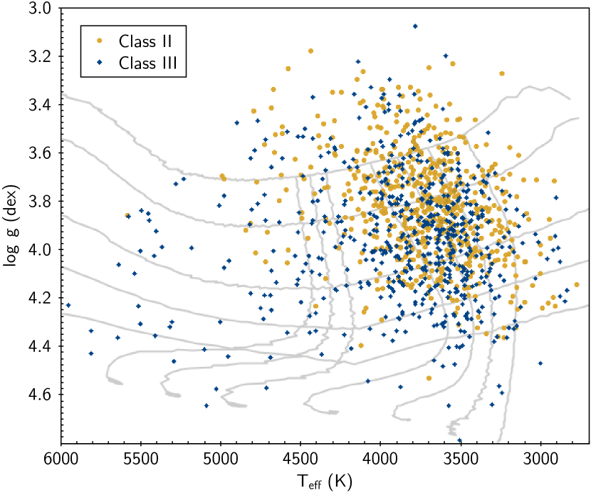
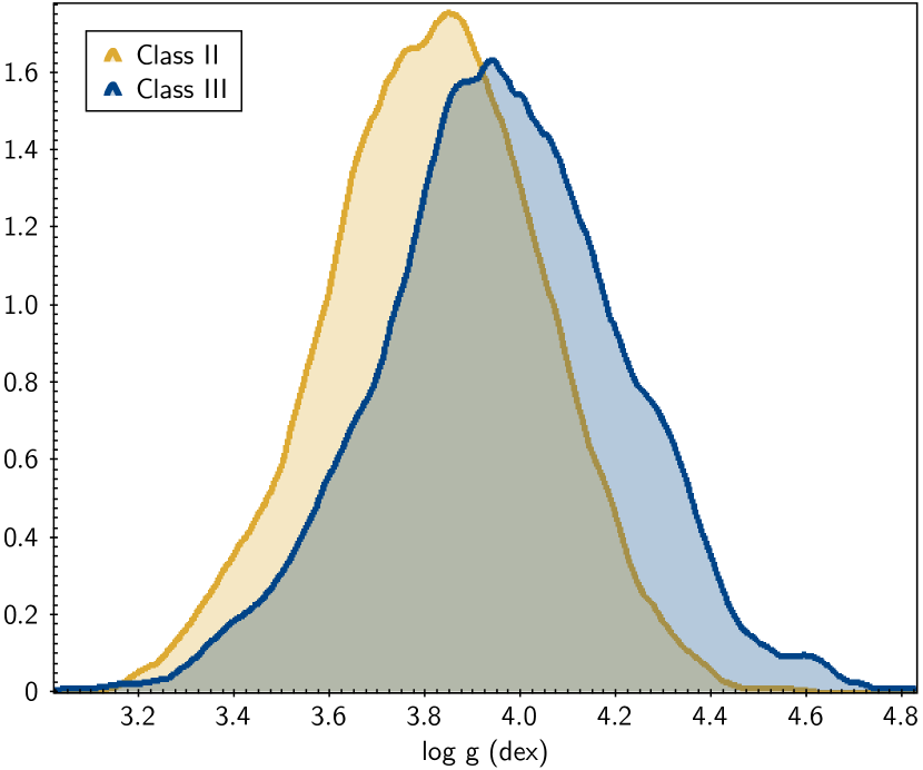
Figure 9: Left: distribution of $T_{eff}$ and $\log g$ for the sources in Orion A shown against 1, 2, 5, 10, and 20 Myr isochrones. Right: Kernel Density Estimation of the $\log g$ with the kernel size of 0.1 dex. Top panels show the three populations identified by Beccari et al. (2017). Middle panels highlight spectroscopic binaries from Kounkel et al. (2019). Bottom panels show the difference in the distribution of disk-bearing Class II YSOs, and diskless Class III photospheres.

In the ONC, Beccari et al. (2017) have observed three distinct populations with the mean ages of 1.2, 1.9 and 2.9 Myr, and that these populations, while overlapping, cover different volume in the sky, with the youngest one being the most centrally concentrated, and the oldest one being the most diffuse. However, they could not rule out that these populations are not due to an unresolved binary and tertiary sequences. Crossmatching against their catalog of sources does indeed show that the these populations are separated in the $\log g$ space, independently confirming different ages (Figure 9, top). While there is some crossover between the sources, the “Very Young” sources peak at $\log g$=3.7 dex, corresponding to $\sim 1$ Myr. The “Young” sources peak at $\log g$=3.9 dex, or at the age of $\sim 2$ Myr, and the “Old” sources peak at $\log g$=4 dex, or at $\sim 3$ Myr, consistent with the original age estimates.

It should be noted, though, that in the full spectroscopic sample, there do not appear to be distinct sequences, rather, the distribution appears to be more continuous. This does not appear to be explained by the smearing of the sequences from the uncertainties. But, examining the density of sources at a given age slices in Figure 8, similarly to Beccari et al. (2017), we do indeed find that the youngest sources are located primarily close to the center of the cluster, while the older stars are more distributed throughout the cluster. A similar trend can also be seen in Perseus, in IC348.

Along the L1641 there are curious chains of coeval stars running in parallel to the cloud. Hacar et al. (2018) have found a large network of gas fibers towards the ONC, any one of which is in process of forming stars along their length, and the stars that would form from the same gas fiber are approximately coeval. Hacar et al. (2016) have previously searched for chains of stars in the APOGEE data in Orion A that are comoving in the position-position-velocity diagram, although the stellar ages have not been considered. Only a few of such chains have been found in L1641, and they did not exhibit any preferential orientation relative to the cloud. It is unclear whether the chains we see in this work is just a chance alignment, or if their arrangement could be thought of as significant.

The derived parameters are not strongly confused by multiplicity - the spectroscopic binaries identified by Kounkel et al. (2019) do not appear to occupy a systematically different $T_{eff}$ or $\log g$ space from other single stars in their corresponding clusters (Figure 9, middle). The uncertainties in the parameters also do not appear to be affected. Metallicity is the only parameter where there might be a slight, barely significant systematic shift, with spectroscopic binaries being on average more metal poor by 0.02 dex.

However, there is a strong difference in $\log g$ as a function of whether a YSO has a protoplanetary disk or not (Figure 9, bottom), with the disk-bearing Class II sources having $\log g$ 0.2 dex lower than their diskless Class III counterparts, although there is much overlap between the two populations. In a given cluster, this effect translates to 1–2 Myr systematic difference in age. A similar separation in $\log g$ has previously been observed by Yao et al. (2018) using the values derived from the IN-SYNC pipeline. It is notable that despite the fact that the aforementioned pipeline does not produce reliable absolute calibration, it does discriminate between the effects of veiling from disks and other spectral parameters. Thus, it is likely that the systematic difference we observe is real and not due to Class II sources being deviating from the model produced by APOGEE Net.

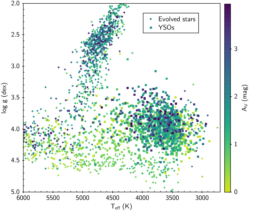
Figure 10:

4.3 Metallicity

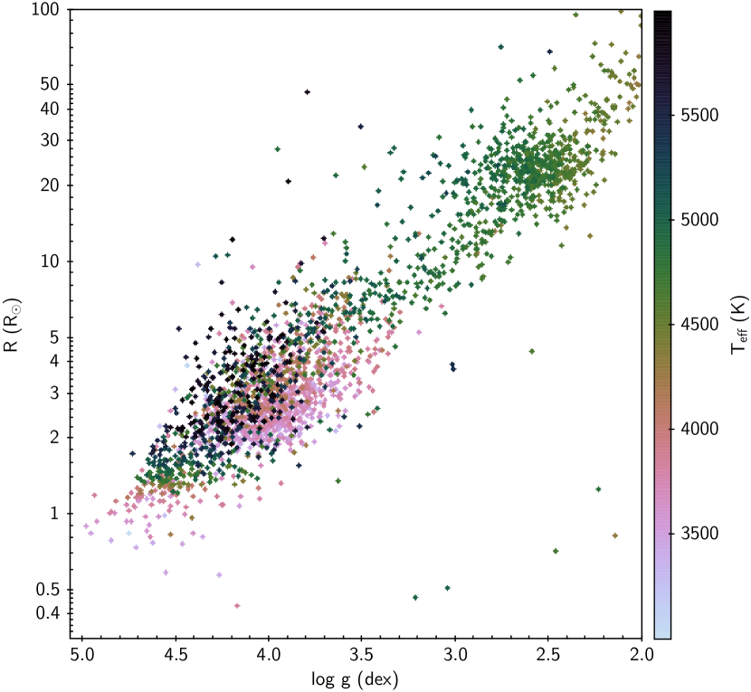
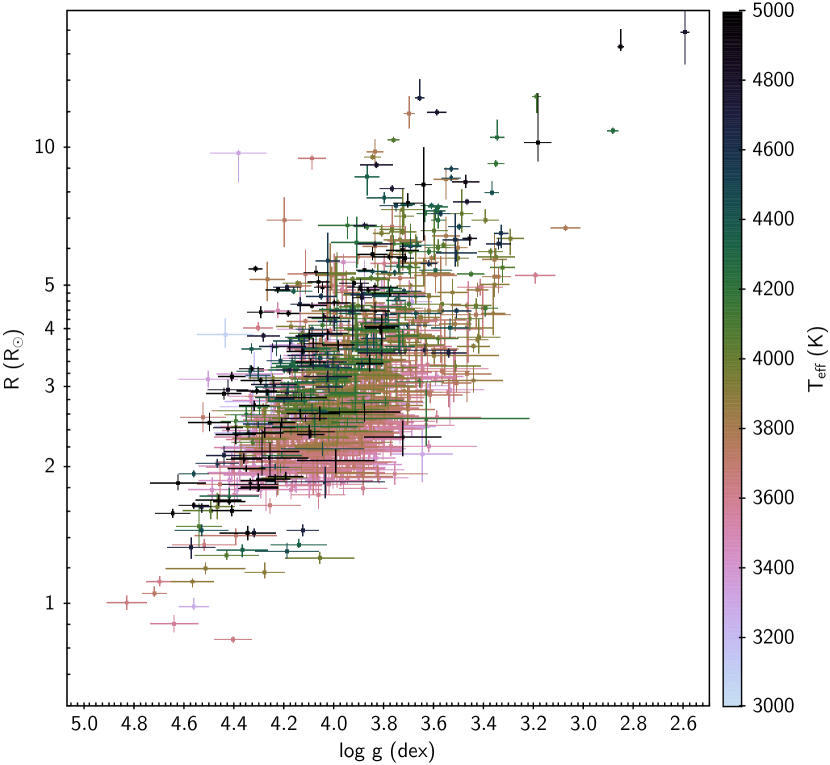
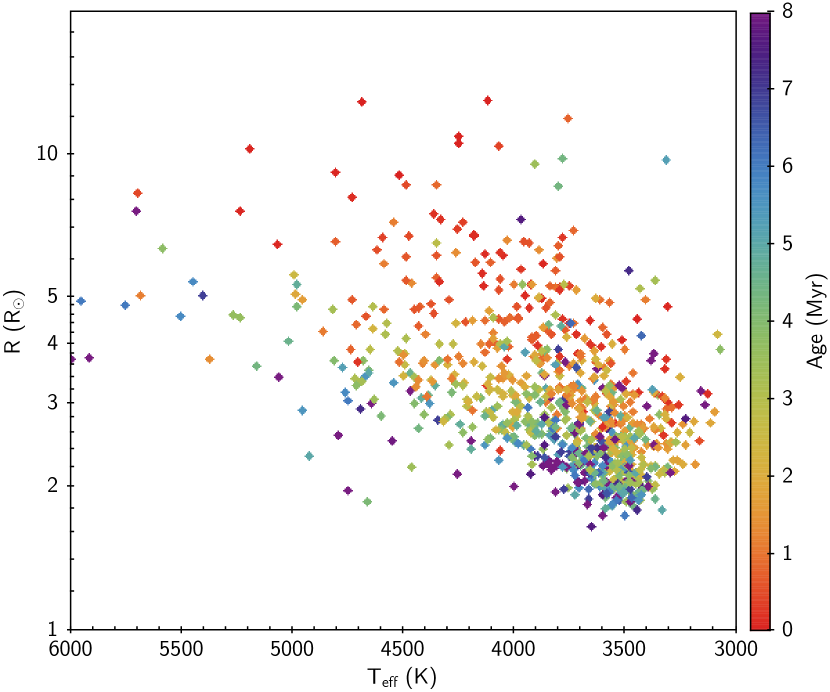
Figure 11:

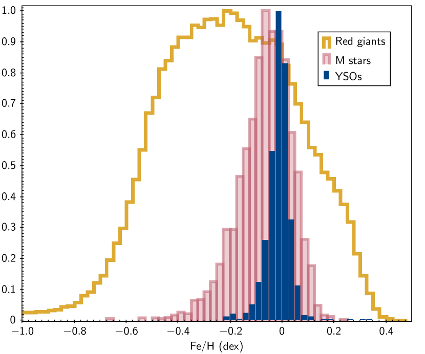
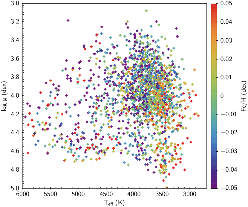
Figure 12:

5 Discussion

Machine learning is an effective approach for classifying stellar spectra, and for the first time we have applied it to spectra of young stars to derive meaningful $T_{eff}$ and $\log g$ that are interpolatable over the isochrones to determine ages. The performance of these parameters can rival the usage of photometric color-magnitude diagrams, offering two major advantages over them – spectroscopic parameters are unaffected by extinction, or by the binary sequence. Using both of these approaches in conjunction with one another could allow for a more detailed analysis of the star forming history inside young populations.

The main limiting factor for machine learning is the existence of reliable input labels over which it would be possible to generalize a particular parameter space. However, it is not necessary to derive those labels from scratch a-priori every single time. Instead, through incremental building on previous efforts, it is possible to improve on even coarse estimates. As the parameter space gets further explored, it may be possible to add other properties to the analysis (e.g., other abundance labels that may be more meaningful in analyzing the chemical content of star forming regions, such as $\alpha$/H), and extend the grid to other type of stars (e.g., with $T_{eff}$$>$8000 K), to produce a fully unified spectral model. Furthermore, if different large spectroscopic surveys with different instruments (having different resolution or different wavelength coverage) have observations of a few sources in common, it would be possible to cross-reference them relative to one another, allowing one to extract stellar parameters in a way that would have fewer systematic offsets.

Appendix A Deep Neural Network Background

Deep neural networks (DNNs) are parameterized functions that map from an input domain to an output domain, and the parameters of which are learned through a training process. While a DNN can be used for both regression and classification tasks, this work is principally concerned with its utility for performing regressions, as stellar parameters are continuous variables.

We are utilizing a particular architecture of DNN known as a convolutional neural network (CNN). The CNN is particularly well-suited for extracting local patterns in spatial data. It has been widely used to achieve state-of-the-art results in various image recognition tasks (Krizhevsky et al., 2012; He et al., 2016; Szegedy et al., 2015; Simonyan & Zisserman, 2014). A CNN typically consists of a sequence of convolutional and pooling layers, followed by a set of fully connected layers. A convolutional layer transforms a subsection of the input, a pooling layer downsamples the input, and a fully connected layer is a classic DNN or multilayer perceptron. Broadly speaking, the convolutional layers can be interpreted as a feature extractors, and the fully connected layers as the predictors. However, this is just an approximation, as the model prediction error is passed back across all its parameters through backpropagation.

A.1 Training via backpropagation

To train a DNN model through backpropagation, it is necessary to use an optimizer and evaluation criteria. In our case we will be using classic stochastic gradient descent for our optimizer. For our evaluation criterion we will be using mean squared error loss (MSE loss).

$$MSE=\frac{1}{N}\sum_{i=1}^{N}\sum_{j=1}^{A}{(Y_{ij}-\hat{Y}_{ij})^{2}}$$ (A1)

in which N is the number of training data points, A is the number of stellar parameters that are considered, Y is a target label, and $\hat{Y}$ is the corresponding model prediction. This loss is then propagated back through the model to produce gradients with respect to each model weight, which are used to update the weights to slightly reduce loss; after enough steps in the direction of the negative gradient, a local minimum is reached.

While the $MSE$ loss sums over all training data points, it is inefficient, and our case infeasible, to load all of the training data into memory at once. Instead, data is usually divided into minibatches, and at each iteration the $MSE$ loss is approximated by summing only over the datapoints in the minibatch. Using gradient descent with these approximate losses is known as stochastic minibatch gradient descent. A full pass through the training set is called an epoch. Typically, the training set is shuffled and after each epoch and re-partitioned into minibatches. In addition to the memory consideration, smaller minibatch sizes and shuffling the training set also have the added benefit of helping to improve model generalization; the randomness in the gradient helps to avoid settling into shallow local minima. However, the smaller the minibatch size is, the more often the parameter weights need to be updated, increasing computational expense.

A.2 Hyperparameters

Machine learning models typically have design parameters that cannot be learned by the network and must be chosen outside of the training process. These “hyperparameters” are typically adjusted by evaluating the model’s performance against the held out development data. The number of datapoints in a minibatch is one such hyperparameter.

Another hyperparameter is the learning rate (also known as step size), the coefficient scaling the gradient used in gradient descent. If the learning rate is too large, the model may fail to converge to a good local minimum. If it is too small, training can be prohibitively slow.

We also treat the dropout rate as a hyperparameter. Dropout is a technique that helps with model generalization by using a mask to zero out a random subset of hidden units during each gradient calculation. This forces the model to distribute the learned representation of the input across all of its hidden units, yielding a more robust internal representation. A dropout rate of 0.1 implies that on any given training pass, 10% of the hidden units on the fully connected layer are masked out: they cannot contribute to the prediction, and gradients will not propagate through them.

Appendix B APOGEE Net Model Code

⬇

class APOGEE_Net(nn.Module):

def __init__(self, num_layers, num_targets, drop_p=0.0):

super(Net, self).__init__()

# 3 input channels, 6 output channels, convolution

# kernel

self.conv1 = nn.Conv1d(num_layers, 8, 3, padding=1)

self.conv2 = nn.Conv1d(8, 8, 3, padding=1)

self.conv3 = nn.Conv1d(8, 16, 3, padding=1)

self.conv4 = nn.Conv1d(16, 16, 3, padding=1)

self.conv5 = nn.Conv1d(16, 16, 3, padding=1)

self.conv6 = nn.Conv1d(16, 16, 3, padding=1)

self.conv7 = nn.Conv1d(16, 32, 3, padding=1)

self.conv8 = nn.Conv1d(32, 32, 3, padding=1)

self.conv9 = nn.Conv1d(32, 32, 3, padding=1)

self.conv10 = nn.Conv1d(32, 32, 3, padding=1)

self.conv11 = nn.Conv1d(32, 64, 3, padding=1)

self.conv12 = nn.Conv1d(64, 64, 3, padding=1)

# an affine operation: y = Wx + b

self.fc1 = nn.Linear(64*133*1, 512)

self.fc1_dropout = nn.Dropout(p=drop_p)

self.fc2 = nn.Linear(512, 512)

self.fc3 = nn.Linear(512, num_targets)

def forward(self, x):

# Max pooling over a (2) window

x = F.max_pool1d(F.relu(self.conv2(F.relu(self.conv1(x)))), 2)

x = F.max_pool1d(F.relu(self.conv4(F.relu(self.conv3(x)))), 2)

x = F.max_pool1d(F.relu(self.conv6(F.relu(self.conv5(x)))), 2)

x = F.max_pool1d(F.relu(self.conv8(F.relu(self.conv7(x)))), 2)

x = F.max_pool1d(F.relu(self.conv10(F.relu(self.conv9(x)))), 2)

x = F.max_pool1d(F.relu(self.conv12(F.relu(self.conv11(x)))), 2)

x = x.view(-1, self.num_flat_features(x))

x = F.relu(self.fc1_dropout(self.fc1(x)))

x = F.relu(self.fc1_dropout(self.fc2(x)))

x = self.fc3(x)

return x

def num_flat_features(self, x):

size = x.size()[1:] # all dimensions except the batch dimension

num_features = 1

for s in size:

num_features *= s

return num_features

References

- Abolfathi et al. (2018) Abolfathi, B., Aguado, D. S., Aguilar, G., et al. 2018, ApJS, 235, 42, doi: 10.3847/1538-4365/aa9e8a
- Anders et al. (2017) Anders, F., Chiappini, C., Minchev, I., et al. 2017, A&A, 600, A70, doi: 10.1051/0004-6361/201629363
- Bailer-Jones (2000) Bailer-Jones, C. A. L. 2000, A&A, 357, 197. https://arxiv.org/abs/astro-ph/0003071
- Bailer-Jones et al. (1997) Bailer-Jones, C. A. L., Irwin, M., Gilmore, G., & von Hippel, T. 1997, MNRAS, 292, 157, doi: 10.1093/mnras/292.1.157
- Baraffe et al. (2015) Baraffe, I., Homeier, D., Allard, F., & Chabrier, G. 2015, A&A, 577, A42, doi: 10.1051/0004-6361/201425481
- Bazarghan & Gupta (2008) Bazarghan, M., & Gupta, R. 2008, Ap&SS, 315, 201, doi: 10.1007/s10509-008-9816-5
- Beccari et al. (2017) Beccari, G., Petr-Gotzens, M. G., Boffin, H. M. J., et al. 2017, A&A, 604, A22, doi: 10.1051/0004-6361/201730432
- Bell (2012) Bell, C. P. M. 2012, PhD thesis, University of Exeter
- Benedict et al. (2016) Benedict, G. F., Henry, T. J., Franz, O. G., et al. 2016, AJ, 152, 141, doi: 10.3847/0004-6256/152/5/141
- Birky et al. (2020) Birky, J., Hogg, D. W., Mann, A. W., & Burgasser, A. 2020, arXiv e-prints, arXiv:2001.04962. https://arxiv.org/abs/2001.04962
- Blanton et al. (2017) Blanton, M. R., Bershady, M. A., Abolfathi, B., et al. 2017, AJ, 154, 28, doi: 10.3847/1538-3881/aa7567
- Bovy et al. (2016) Bovy, J., Rix, H.-W., Schlafly, E. F., et al. 2016, ApJ, 823, 30, doi: 10.3847/0004-637X/823/1/30
- Buder et al. (2018) Buder, S., Asplund, M., Duong, L., et al. 2018, MNRAS, 478, 4513, doi: 10.1093/mnras/sty1281
- Cargile et al. (2019) Cargile, P. A., Conroy, C., Johnson, B. D., et al. 2019, arXiv e-prints, arXiv:1907.07690. https://arxiv.org/abs/1907.07690
- Choi et al. (2016) Choi, J., Dotter, A., Conroy, C., et al. 2016, ApJ, 823, 102, doi: 10.3847/0004-637X/823/2/102
- Cottaar et al. (2014) Cottaar, M., Covey, K. R., Meyer, M. R., et al. 2014, ApJ, 794, 125, doi: 10.1088/0004-637X/794/2/125
- Cottaar et al. (2015) Cottaar, M., Covey, K. R., Foster, J. B., et al. 2015, ApJ, 807, 27, doi: 10.1088/0004-637X/807/1/27
- Covey et al. (2016) Covey, K. R., Agüeros, M. A., Law, N. M., et al. 2016, ApJ, 822, 81, doi: 10.3847/0004-637X/822/2/81
- Da Rio et al. (2016) Da Rio, N., Tan, J. C., Covey, K. R., et al. 2016, ApJ, 818, 59, doi: 10.3847/0004-637X/818/1/59
- Da Rio et al. (2017) —. 2017, ApJ, 845, 105, doi: 10.3847/1538-4357/aa7a5b
- Doppmann et al. (2005) Doppmann, G. W., Greene, T. P., Covey, K. R., & Lada, C. J. 2005, AJ, 130, 1145, doi: 10.1086/431954
- D’Orazi et al. (2011) D’Orazi, V., Biazzo, K., & Randich, S. 2011, A&A, 526, A103, doi: 10.1051/0004-6361/201015616
- D’Orazi et al. (2009) D’Orazi, V., Randich, S., Flaccomio, E., et al. 2009, A&A, 501, 973, doi: 10.1051/0004-6361/200811241
- Fabbro et al. (2018) Fabbro, S., Venn, K. A., O’Briain, T., et al. 2018, MNRAS, 475, 2978, doi: 10.1093/mnras/stx3298
- Foster et al. (2015) Foster, J. B., Cottaar, M., Covey, K. R., et al. 2015, ApJ, 799, 136, doi: 10.1088/0004-637X/799/2/136
- Gaia Collaboration et al. (2018) Gaia Collaboration, Brown, A. G. A., Vallenari, A., et al. 2018, A&A, 616, A1, doi: 10.1051/0004-6361/201833051
- García Pérez et al. (2016) García Pérez, A. E., Allende Prieto, C., Holtzman, J. A., et al. 2016, AJ, 151, 144, doi: 10.3847/0004-6256/151/6/144
- Gunn et al. (2006) Gunn, J. E., Siegmund, W. A., Mannery, E. J., et al. 2006, AJ, 131, 2332, doi: 10.1086/500975
- Hacar et al. (2016) Hacar, A., Alves, J., Forbrich, J., et al. 2016, A&A, 589, A80, doi: 10.1051/0004-6361/201527805
- Hacar et al. (2018) Hacar, A., Tafalla, M., Forbrich, J., et al. 2018, A&A, 610, A77, doi: 10.1051/0004-6361/201731894
- Hayden et al. (2015) Hayden, M. R., Bovy, J., Holtzman, J. A., et al. 2015, ApJ, 808, 132, doi: 10.1088/0004-637X/808/2/132
- He et al. (2016) He, K., Zhang, X., Ren, S., & Sun, J. 2016, in Proceedings of the IEEE conference on computer vision and pattern recognition, 770–778
- Hejazi et al. (2015) Hejazi, N., De Robertis, M. M., & Dawson, P. C. 2015, AJ, 149, 140, doi: 10.1088/0004-6256/149/4/140
- Holtzman et al. (2015) Holtzman, J. A., Shetrone, M., Johnson, J. A., et al. 2015, AJ, 150, 148, doi: 10.1088/0004-6256/150/5/148
- Kounkel et al. (2018) Kounkel, M., Covey, K., Suárez, G., et al. 2018, AJ, 156, 84, doi: 10.3847/1538-3881/aad1f1
- Kounkel et al. (2019) Kounkel, M., Covey, K., Moe, M., et al. 2019, AJ, 157, 196, doi: 10.3847/1538-3881/ab13b1
- Krizhevsky et al. (2012) Krizhevsky, A., Sutskever, I., & Hinton, G. E. 2012, in Advances in neural information processing systems, 1097–1105
- Kunder et al. (2017) Kunder, A., Kordopatis, G., Steinmetz, M., et al. 2017, AJ, 153, 75, doi: 10.3847/1538-3881/153/2/75
- Leung & Bovy (2019) Leung, H. W., & Bovy, J. 2019, MNRAS, 483, 3255, doi: 10.1093/mnras/sty3217
- Majewski et al. (2017) Majewski, S. R., Schiavon, R. P., Frinchaboy, P. M., et al. 2017, AJ, 154, 94, doi: 10.3847/1538-3881/aa784d
- Mann et al. (2015) Mann, A. W., Feiden, G. A., Gaidos, E., Boyajian, T., & von Braun, K. 2015, ApJ, 804, 64, doi: 10.1088/0004-637X/804/1/64
- Marigo et al. (2017) Marigo, P., Girardi, L., Bressan, A., et al. 2017, ApJ, 835, 77, doi: 10.3847/1538-4357/835/1/77
- Ness et al. (2015) Ness, M., Hogg, D. W., Rix, H. W., Ho, A. Y. Q., & Zasowski, G. 2015, ApJ, 808, 16, doi: 10.1088/0004-637X/808/1/16
- Nidever et al. (2015) Nidever, D. L., Holtzman, J. A., Allende Prieto, C., et al. 2015, AJ, 150, 173, doi: 10.1088/0004-6256/150/6/173
- Paszke et al. (2017) Paszke, A., Gross, S., Chintala, S., et al. 2017, in NIPS-W
- Schlafly & Finkbeiner (2011) Schlafly, E. F., & Finkbeiner, D. P. 2011, ApJ, 737, 103, doi: 10.1088/0004-637X/737/2/103
- Sharma et al. (2019) Sharma, K., Kembhavi, A., Kembhavi, A., et al. 2019, arXiv e-prints, arXiv:1909.05459. https://arxiv.org/abs/1909.05459
- Simonyan & Zisserman (2014) Simonyan, K., & Zisserman, A. 2014, arXiv e-prints, arXiv:1409.1556. https://arxiv.org/abs/1409.1556
- Simonyan & Zisserman (2014) Simonyan, K., & Zisserman, A. 2014, Very Deep Convolutional Networks for Large-Scale Image Recognition. https://arxiv.org/abs/1409.1556
- Stassun et al. (2017) Stassun, K. G., Collins, K. A., & Gaudi, B. S. 2017, AJ, 153, 136, doi: 10.3847/1538-3881/aa5df3
- Stauffer et al. (1998) Stauffer, J. R., Schultz, G., & Kirkpatrick, J. D. 1998, ApJ, 499, L199, doi: 10.1086/311379
- Szegedy et al. (2015) Szegedy, C., Liu, W., Jia, Y., et al. 2015, in Proceedings of the IEEE conference on computer vision and pattern recognition, 1–9
- Ting et al. (2019) Ting, Y.-S., Conroy, C., Rix, H.-W., & Cargile, P. 2019, ApJ, 879, 69, doi: 10.3847/1538-4357/ab2331
- Veyette et al. (2017) Veyette, M. J., Muirhead, P. S., Mann, A. W., et al. 2017, ApJ, 851, 26, doi: 10.3847/1538-4357/aa96aa
- Wilson et al. (2010) Wilson, J. C., Hearty, F., Skrutskie, M. F., et al. 2010, in Proc. SPIE, Vol. 7735, Ground-based and Airborne Instrumentation for Astronomy III, 77351C, doi: 10.1117/12.856708
- Yao et al. (2018) Yao, Y., Meyer, M. R., Covey, K. R., Tan, J. C., & Da Rio, N. 2018, ApJ, 869, 72, doi: 10.3847/1538-4357/aaec7a
- Zasowski et al. (2017) Zasowski, G., Cohen, R. E., Chojnowski, S. D., et al. 2017, AJ, 154, 198, doi: 10.3847/1538-3881/aa8df9