KdV-charged black holes

Abstract

We construct black hole geometries in AdS₃ with non-trivial values of KdV charges. The black holes are holographically dual to quantum KdV Generalized Gibbs Ensemble in 2d CFT. They satisfy thermodynamic identity and thus are saddle point configurations of the Euclidean gravity path integral. We discuss holographic calculation of the KdV generalized partition function and show that for a certain value of chemical potentials new geometries, not the conventional BTZ ones, are the leading saddles.

1 Introduction

Thermalization and non-equilibrium dynamics in two-dimensional conformal field theory is a rich subject touching on many topics of contemporary interest, from cold atom experiments to chaos in quantum gravity calabrese2006time ; calabrese2007quantum ; Roberts:2014ifa . Dynamics of 2d CFTs is constrained by presence of an infinite tower of local conserved quantum KdV charges $\hat{Q}_{2k+1}$, which commute with each other and the CFT Hamiltonian $\hat{Q}_{1}=L_{0}-c/24$. The qKdV integrable structure of 2d CFTs has been actively studied in the past bazhanov1996integrable ; bazhanov1997integrable ; bazhanov1999integrable ; bazhanov97zero , as well as more recently maloney2018thermal ; Kotousov:2019nvt ; LeFloch:2019wlf .

Interest in quantum KdV charges was rekindled recently in the context of generalized thermalization of quantum integrable systems and Generalized Gibbs Ensemble, which is expected to emerge as a result of thermalization dynamics vidmar2016generalized . In particular, if the initial 2d CFT state carries non-trivial qKdV charges, local physics at late times was argued to be given by the KdV GGE state cardy2016quantum ,

$$\rho_{\rm GGE}=e^{-\sum_{k}\tilde{\mu}_{k}\hat{Q}_{2k+1}}/{\mathcal{Z}},$$ (1)

where

$${\mathcal{Z}}={\rm Tr}\,e^{-\sum_{k}\tilde{\mu}_{k}\hat{Q}_{2k+1}}$$ (2)

is the KdV generalized partition function. Thermodynamics and other basic properties of the KdV GGE are not well understood. In fact $\mathcal{Z}$ is not known explicitly even for simplest theories. This paper is paving the way for calculation of ${\mathcal{Z}}$ in the large $c$ limit. In the previous works on the subject, both on holographic and the CFT sides de2016remarks ; maloney2018generalized ; GGE ; GGE2 , it was implicitly assumed that the BTZ black holes, i.e. eigenstates of $\hat{Q}_{1}=L_{0}-c/24$ on the CFT side, are the leading saddle point configurations contributing to the KdV generalized partition function (2). Provided this is the case, $1/c$ corrections can be calculated by quantizing small fluctuations near the BTZ saddle, as was done on the CFT side in GGE2 . We show this is not always the case, namely there are novel black hole configurations, which correspond to complicated CFT states, not $\hat{Q}_{1}$ eigenstates, which are leading contributions to ${\mathcal{Z}}$, at least for the particular values of chemical potentials $\tilde{\mu}_{2k+1}$.

These KdV-charged black holes, which we construct explicitly, are gravity dual to the KdV GGE state (1). Conventional BTZ geometries emerge as a particular case, which is dual to the conventional Gibbs Ensemble, i.e. when all $\tilde{\mu}_{2k+1}=0$ except for $\tilde{\mu}_{1}=\beta$.

The mapping between a particular KdV-charged black hole and (1) is non-trivial. Namely, the averaged values of $\hat{Q}_{2k+1}$ in $\rho_{\rm GGE}$ should match those in the holographic configuration. Thus, at infinite $c$, corresponding classical black hole geometry analytically continued to Euclidean signature should be a leading saddle point configuration of the corresponding gravity path integral evaluating $\mathcal{Z}$. To support the validity of this prescription, we explicitly show for a particular simple KdV-charged configuration that for the certain values of $\tilde{\mu}_{2k+1}$ its contribution exceeds those of the BTZ black holes.

We provide a general proof that the KdV-charged black holes satisfy the first law of thermodynamics. This and other properties of the geometries follow from the integrable structure of the KdV equation and its relation to the co-adjoint orbit of Virasoro algebra. To make the presentation self-contained, we start with a succinct introduction of mathematical preliminaries in the next section. After that, in section 3, we explain how classical integrability of KdV equation gives rise to quantum KdV charges in 2d CFTs. The new geometrical solutions are constructed and analyzed in section 4, where we also prove the thermodynamic identity. Section 5 discusses dual field theory interpretation of the new geometries. In section 6 we calculate KdV generalized partition function $\mathcal{Z}$ on the gravity side in the case when only $\tilde{\mu}_{1}$, and $\tilde{\mu}_{3}$ are non-zero, and see that only thermal AdS and BTZ configurations contribute. Then in section 7 we turn on $\tilde{\mu}_{5}$ and see that new KdV-charged black hole configurations appear and may become leading for a particular range of parameters. We conclude with a discussion in section 8.

2 Mathematical preliminaries

In this section we provide mathematical preliminaries necessary for the general discussion of the consecutive sections. We aimed at a self-contained but concise presentation and many details and proofs were omitted. The reader is advised to consult the original papers by Witten, Novikov, and others Witten:1987ty ; novikov1974periodic ; lazutkin1975normal ; dubrovin1974periodicity ; novikov1984theory for a systematic presentation of the geometry of the co-adjoint orbits of Virasoro algebra, finite-zone solutions of the generalized KdV equations, and other related questions.

2.1 Co-adjoint orbit of Virasoro algebra

We start by introducing the group ${\rm diff}\,\mathbb{S}^{1}$ of diffeomorphisms of a circle. Elements of ${\rm diff}\,\mathbb{S}^{1}$ are monotonically increasing functions $\tilde{\varphi}=g(\varphi)$,

$$g(2\pi)=g(0)+2\pi,$$ (3)

such that $g$ is an invertible map of a circle into itself, $g(\varphi)=g(\varphi^{\prime})\Rightarrow\varphi=\varphi^{\prime}$. Corresponding Lie algebra is the Witt algebra of vector fields on a circle $f(\varphi)\partial_{\varphi}$.

Next we consider a periodic “potential” $u(\varphi)$, $u(\varphi+2\pi)=u(\varphi)$ and a “wave-function” $\psi(\varphi)$ satisfying “Schr$\ddot{\rm o}$dinger” equation (properly called Hill’s equation),

$$-\psi^{\prime\prime}+{u\over 4}\,\psi=0.$$ (4)

Diffeomorphisms $g\in{\rm diff}\,\mathbb{S}^{1}$ naturally act on $u$ and $\psi$,

$$g: \psi(\varphi)\rightarrow\tilde{\psi}(\tilde{\varphi}),$$ (5)

$$g: u(\varphi)\rightarrow\tilde{u}(\tilde{\varphi}),$$ (6)

such that the Hill’s equation continue being satisfied (the derivative is with respect to $\tilde{\varphi}$),

$$-\tilde{\psi}^{\prime\prime}+{\tilde{u}\over 4}\,\tilde{\psi}=0.$$ (7)

The new potential and the new wave-function are defined via

$$\tilde{\psi}(\tilde{\varphi}(\varphi)) = \psi(\varphi)\left({d\tilde{\varphi}\over d\varphi}\right)^{1/2},$$ (8)

$$\tilde{u}(\tilde{\varphi}(\varphi)) = \left({d\tilde{\varphi}\over d\varphi}\right)^{-2}\left[u(\varphi)+2\{\tilde{\varphi},\varphi\}\right].$$ (9)

Here for any $\theta(\varphi)$

$$\{\theta,\varphi\}\equiv{\theta^{\prime\prime\prime}\over\theta^{\prime}}-{3\over 2}\left({\theta^{\prime\prime}\over\theta^{\prime}}\right)^{2},$$ (10)

is the Schwarzian derivative.

An infinitesimal transformation

$$g(\varphi)=\varphi-\epsilon f(\varphi)$$ (11)

acts on the potential as follows,

$$\tilde{u}(\varphi)=u(\varphi)+\epsilon\,\mathcal{D}f,\qquad\mathcal{D}\equiv(\partial u)+2u\partial-2\,\partial^{3}.$$ (12)

As we will now see, this is the action of Virasoro algebra, central extension of Witt algebra, on its co-adjoint orbit.

Elements of Virasoro algebra are the pairs $(f,a)$ where $f$ is a vector field and $a$ is a $\mathbb{C}$-number with the following commutation relation

$$[(f_{1},a_{1}),(f_{2},a_{2})]=(f_{1}f_{2}^{\prime}-f_{1}^{\prime}f_{2},a),\qquad a=\int_{0}^{2\pi}d\varphi(f_{1}^{\prime\prime\prime}f_{2}-f_{1}f_{2}^{\prime\prime\prime}).$$ (13)

Co-adjoint space is the linear space dual to the algebra. Its elements are the pairs $[u,\hat{t}]$ where $u(\varphi)d\varphi^{2}$ is a “two-differential” and $[0,\hat{t}]$ is an element formally dual to $(0,1)$. We want $\hat{t}$ to be common for all elements, and therefore we can reduce the notations from $[u,\hat{t}]$ to simply $u$, such that the scalar product is

$$\langle(f,a),u\rangle=a+\int_{0}^{2\pi}d\varphi\,uf.$$ (14)

It is easy to see that $\langle(f,a),u\rangle$ is invariant under the action of a Virasoro algebra element $(v,b)$ provided,

$$\delta f=vf^{\prime}-v^{\prime}f,\quad\delta a=\int_{0}^{2\pi}d\varphi(v^{\prime\prime\prime}f-vf^{\prime\prime\prime}),\quad\delta u=\mathcal{D}v.$$ (15)

Action of ${{\rm diff}\,\mathbb{S}^{1}}$ (15) foliates the space of all $u(\varphi)$ into orbits – the co-adjoint orbits of Virasoro algebra. Starting with some potential $u$ one defines a sub-algebra of stabilizers $f$ of $u$ such that

$$\delta u=\mathcal{D}f=0.$$ (16)

In full generality there could be either one or three linearly independent stabilizers Witten:1987ty , which must be closed in the Lie algebra sense. Then the orbit is defined by the action of all possible diffeomorphisms $g(\varphi)$ on the given $u$, modulo the stabilizer subgroup. The simplest orbit is obtained starting from a constant $u(\varphi)=u_{0}$. In this case the stabilizer is unique, $f=1$, up to an overall rescaling, with an exception of the case when $u_{0}\neq-n^{2}$ for some integer $n$. These are the orbits ${\rm diff}\,\mathbb{S}^{1}/\mathbb{S}^{1}$ in the notations of Witten Witten:1987ty , or stable orbits in the notations of Lazutkin and Pankratova lazutkin1975normal . Quantization of such an orbit gives rise to Verma module.

When $u(\varphi)$ belongs to an orbit ${\rm diff}\,\mathbb{S}^{1}/\mathbb{S}^{1}$ the stabilizer vector field $f$ for each $u$ is unique and sign-definite. The converse is also correct and easy to see. Let us consider $f$, such that it is sign-definite and $\mathcal{D}f=0$. We first notice that

$$2\pi f_{0}^{-1}=\int_{0}^{2\pi}{d\varphi\over f},$$ (17)

is invariant under the diffeomorphism ${\rm diff}\,\mathbb{S}^{1}$, as follows straightforwardly from (13). Next, one can define the diffeomorphism $\varphi\rightarrow\tilde{\varphi}=g(\varphi)$,

$$d\tilde{\varphi}=f_{0}{d\varphi\over f},$$ (18)

which brings $f$ to a constant form $f_{0}$. This is the diffeomorphism which brings $u(\varphi)$ to a constant, as follows from applying (9),

$$\tilde{u}(\tilde{\varphi})=u_{0}={uf^{2}+f^{\prime 2}-2ff^{\prime\prime}\over f_{0}^{2}}.$$ (19)

That $u_{0}$ is a constant can be verified by differentiating it, $\tilde{u}^{\prime}=(f/f_{0})\partial_{\varphi}u_{0}=(f^{2}/f_{0}^{3})\mathcal{D}f=0$. An alternative way to obtain the same expression is to start with $\mathcal{D}f=0$ and solve it as an equation for $u$,

$$u(\varphi)={u_{0}f_{0}^{2}-f^{\prime 2}+2ff^{\prime\prime}\over f^{2}}.$$ (20)

Here $u_{0}f_{0}^{2}$ appears as an integration constant. It is straightforward to see that (20) is compatible with (15) only if $u_{0}f_{0}^{2}$ is invariant under the diffeomorphisms. Hence $u_{0}f_{0}^{2}$ is equal to $uf^{2}$ when $u(\varphi)$ is $\varphi$-independent and hence so is $f$. Finally, we note that $u_{0}$ is the only invariant characterizing the orbit, and its invariance under the diffeomorphisms follows straightforwardly from (19) and (13).

The space of all potentials is a Poisson manifold with the Poisson bracket magri1978simple ,

$${c\over 24}\{u(\varphi_{1}),u(\varphi_{2})\}=-2\pi\mathcal{D}\delta(\varphi_{1}-\varphi_{2}),$$ (21)

where $c$ is some numerical parameter. Written in terms of the Fourier series

$${c\over 24}(u(\varphi)+1)=\sum_{k}\ell_{k}e^{ik\varphi},$$ (22)

the Poisson brackets (21) reduce to Virasoro algebra

$$i\{\ell_{n},\ell_{m}\}=(n-m)\ell_{n+m}+{c(n^{3}-n)\over 12}\delta_{n+m}.$$ (23)

In particular for any functional ${\mathcal{H}}[u(\varphi)]$,

$${c\over 24}\{{\mathcal{H}},u(x)\}=\mathcal{D}f,\qquad f=2\pi{\delta{\mathcal{H}}\over\delta u(x)}.$$ (24)

Here $\mathcal{D}f$ is as the Hamiltonian vector field associated with $\mathcal{H}$ in the space of potentials $u(\varphi)$.

Since the Hamiltonian vector field (24) has the form of (15) with some appropriate $v=f$, Hamiltonian flow does not move $u(x)$ away from the orbit, hence on the space of all potentials the Poisson bracket is degenerate. Restricting it to a particular orbit removes this degeneracy, and (21) defines a symplectic form, such that each orbit is a symplectic manifold. This symplectic form is the Kirillov-Kostant form on the co-adjoint orbit of Virasoro algebra gervais1982dual , as is also evident from (23).

2.2 KdV hierarchy

We now go back to Hill’s equation (4) and extend it to a full Schr$\ddot{\rm o}$dinger eigenvalue problem (Sturm-Liouville equation),

$$-\psi^{\prime\prime}+{u\over 4}\psi=\lambda\,\psi.$$ (25)

The (non-degenerate) eigenvalues of periodic $\psi(2\pi)=\psi(0)$ and anti-periodic $\psi(2\pi)=-\psi(0)$ problems constitute the so-called spectral data of $u(\varphi)$. Different potentials may share the same spectral data. In fact there is an infinite family of infinitesimal deformations which are isospectral, i.e. preserve the spectral data. The isospectral deformations are generated by the Hamiltonian flow associated with the Poisson bracket (21),

$$\delta u={c\over 24}\{Q_{2k-1},u\},$$ (26)

where $Q_{2k-1}$ are the so-called KdV generators, which can be defined iteratively,

$$Q_{2k-1}={1\over 2\pi}\int_{0}^{2\pi}d\varphi\,R_{k},\qquad\partial R_{k+1}={k+1\over 2k+1}\mathcal{D}R_{k},\qquad R_{0}=1.$$ (27)

The Gelfand-Dikii polynomials $R_{k}$ gel1975asymptotic satisfy various relations, in particular

$${c\over 24}\{Q_{2k-1},u\}=(2k-1)\partial R_{k}.$$ (28)

First few $R_{k}$ and $Q_{2k-1}$ are given by

$$R_{0} = 1,\quad R_{1}=u,\quad R_{2}=u^{2}-{4\over 3}\partial^{2}u,\quad R_{3}=u^{3}-4u\partial^{2}u-2(\partial u)^{2}+{8\over 5}\partial^{4}u,\qquad$$ (29)

$$I_{0} = u,\quad I_{1}={u^{2}},\quad I_{2}={u^{3}+2(\partial u)^{2}},\quad I_{3}={u^{4}}+8u(\partial u)^{2}+{16(\partial^{2}u)^{2}\over 5},$$ (30)

where $2\pi\,Q_{2k+1}=\int_{0}^{2\pi}d\varphi\,I_{k}$. Of course $I_{k}$ and $R_{k+1}$ differ only by a full derivative.

The name KdV comes from the form of the flow generated by $Q_{3}$. Assuming it defines a $t$-dependent function $u(t,x)$ via

$$\dot{u}={c\over 24}\{Q_{3},u\}=6uu^{\prime}-{4}u^{\prime\prime\prime},$$ (31)

we immediately recognize the original KdV equation (perhaps up to a notational difference).

The KdV charges are in involution, $\{Q_{2k-1},Q_{2l-1}\}=0$, yet the action of $Q_{2k-1}$ on a given $u(x)$ is usually non-trivial. It is known that the corresponding Hamiltonian flows exhaust all possible isospectral deformations.

2.3 Finite-zone “Novikov” solutions

For an arbitrary complex $\lambda$ equation (25) has two solutions, which can be combined into a complex-valued quasi-periodic wave-function

$$\psi(\varphi+2\pi)=\psi(\varphi)e^{2\pi ip(\lambda)}.$$ (32)

For real $\lambda$ the quasi-momentum $p(\lambda)$ is either real or pure imaginary. In the latter case $\lambda$ belongs to the so-called forbidden zone. Forbidden zones stretch between two consecutive eigenvalues of periodic or anti-periodic problem. The zone disappears if the periodic or anti-periodic problem is double degenerate. The quasi-momentum is a complex function with the branch-cuts along the forbidden zones and $\lambda\leq\lambda_{0}$, where $\lambda_{0}$ is the energy of the ground state. For example all eigenvalue of the periodic and antiperiodic problems for the constant potential $u=u_{0}$ are double degenerate (except for the ground state),

$$\lambda^{(n)}={n^{2}+u_{0}\over 4},\qquad n\geq 0.$$ (33)

Therefore there are no forbidden zones and $p(\lambda)=\sqrt{\lambda-u_{0}/4}$.

A special class of potentials with only a finite number of degeneracies lifted, and hence only a finite number of forbidden zones, are called finite-zone potentials. For example a one-zone potential will have a double-degenerate eigenvalue $\lambda^{(k)}$ for some $k\geq 1$ split into two, $\lambda^{(k)}_{-}=\lambda_{1}$ and $\lambda^{(k)}_{+}=\lambda_{2}$, while all other eigenvalues of periodic and antiperiodic problems remain double-degenerate (although their values are no longer given by (33)). It turns out that the values of all double-degenerate eigenvalues are uniquely fixed by the vacuum energy $\lambda_{0}$ and the ends of the zones, which in our case are $\lambda_{1},\lambda_{2}$. Corresponding $p(\lambda)$ has two branch-cuts from $-\infty$ to $\lambda_{0}$ and from $\lambda_{1}$ to $\lambda_{2}$ and is given by an Elliptic integral discussed below. It is naturally defined on a torus, a Riemann curve of genus $1$. More generally a finite zone potential is specified by $\lambda_{i}$, $0\leq i\leq 2n$ and is defined on a hyperelliptic curve of genus $n$.

Finite-zone potentials emerge as solutions of the static generalized KdV equation novikov1974periodic ,

$$\{{\mathcal{H}},u\}=0,\qquad{\mathcal{H}}=\sum_{i=0}^{n}\mu_{2i+1}Q_{2i+1},\qquad\mu_{2n+1}\neq 0.$$ (34)

In fact the following is true. Any solution of (34) is a $m\leq n$-zone potential, and all $n$-zone potentials can be obtained from (34) with the appropriate $\mu_{2i+1}$.

For the given spectral data specified by the ends of the zones $\lambda_{i}$, $0\leq i\leq 2n$, quasi-momentum is specified indirectly by its differential

$$dp={\lambda^{n}+r_{n-1}\lambda^{n-1}+\dots r_{0}\over 2y}d\lambda,$$ (35)

which is defined on the Riemann curve

$$y^{2}=\prod_{i=0}^{2n}(\lambda-\lambda_{i}).$$ (36)

Coefficients $r_{i}$ are fixed by the condition that

$$\oint\limits_{a_{i}}dp=2\int_{\lambda_{2i-1}}^{\lambda_{2i}}dp=0,$$ (37)

vanishes for any a-cycle, defined as the brunch-cuts of $y$ from $\lambda_{2i-1}$ to $\lambda_{2i}$. Because of (37), function $p(\lambda)$ defined such that $dp=({\partial p}/\partial\lambda)d\lambda$ is a well defined function on the Riemann curve (36).

As a complex function $p(\lambda)$ has branch-cuts along the forbidden zones, and therefore finite zone solutions are also called finite- or multi-cut solutions, the language we occasionally use in this paper.

Each Hamiltonian flow generated by $Q_{2k+1}$ is isospectral, hence it deforms a finite-zone solution into another, such that $\{{\mathcal{H}},u\}=0$ continue being satisfied. For any fixed $Q_{2k-1}$, $1\leq k\leq n+1$, values of all higher charges $Q_{2k-1}$, $k>n+1$ are fixed and the space of solutions is an $n$-dimensional torus (Jacobian of the hyperelliptic curve (36)). All charges $Q_{2k+1}$ generate a flow on the Jacobian, which is ergodic in a general case. The exception being the flow generated by $Q_{1}$ which is equivalent to the shift $\varphi\rightarrow\varphi+{\rm const}$ and therefore $2\pi$-periodic.

Spectral data is not invariant under ${\rm diff}\,\mathbb{S}^{1}$ transformations (9), but $\lambda=0$ quasi-periodic eigenfunction $\psi$ transforms into $\tilde{\psi}$ according to (8), which is different only by an overall $2\pi$-periodic factor. Hence $e^{2\pi ip(0)}$ is an invariant on the whole co-adjoint orbit. Considering a constant representative $u(\varphi)=u_{0}$ yields

$$u_{0}=-4p^{2}(0).$$ (38)

2.4 Example: one-cut solutions

In this section we solve the generalized KdV equation (34) for $n=1$,

$$\frac{c}{24}\{Q_{3}+\alpha\,Q_{1},u\}=6u\,u^{\prime}-4u^{\prime\prime\prime}+\alpha\,u^{\prime}=0.$$ (39)

By integrating this equation twice we obtain an effective problem for a particle moving in a cubic potential

$${u^{\prime 2}\over 2}+V(u)=E,\quad 2(E-V)={1\over 2}(u-u_{1})(u-u_{2})(u-u_{3}),$$ (40)

$$s1:=u_{1}+u_{2}+u_{3}=-\alpha/2.$$ (41)

Two out of three parameters $u_{i}$ are free. They specify the values of $Q_{1},Q_{3}$ evaluated on the solution. From (40) $u(\varphi)$ can be obtained easily in terms of Weierstrass’s elliptic function $\wp$ by specifying the initial condition $u(\varphi_{0})$. We require the solution to be $2\pi$-periodic, which imposes a condition on “energy” $E$, leaving only one free parameter, besides $\varphi_{0}$. There is in fact an infinite tower of solutions with the period $2\pi/k$ for positive integer $k$, each being parametrized by one continuous parameter, in addition to $\varphi_{0}$. Weierstrass’s function is associated with a torus, and we choose $s_{1}$ and torus modular parameter $q=e^{i\pi\tau}$ as the independent parameter of one-cute solution,

$$u_{1}={s_{1}\over 3}-{2k^{2}\over 3}\left(\theta_{2}(0;q)^{4}+\theta_{3}(0;q)^{4}\right),$$ (42)

$$u_{2}={s_{1}\over 3}+{2k^{2}\over 3}\left(\theta_{2}(0;q)^{4}-\theta_{4}(0;q)^{4}\right),$$ (43)

$$u_{3}={s_{1}\over 3}+{2k^{2}\over 3}\left(\theta_{3}(0;q)^{4}+\theta_{4}(0;q)^{4}\right).$$ (44)

We order $u_{1}\leq u_{2}\leq u_{3}$, such that the periodic solution describes the oscillations of a “particle” between $u_{1}$ and $u_{2}$. Sometimes instead of $u_{i}$ it is convenient to use $s_{1}$ and

$$s_{2} := u_{1}u_{2}+u_{2}u_{3}+u_{1}u_{3}=-{k^{4}\over\pi^{4}}g_{2}(\tau)+{s_{1}^{2}\over 3},$$ (45)

$$s_{3} := u_{1}u_{2}u_{3}=-{2k^{6}\over\pi^{6}}g_{3}(\tau)-{k^{4}\over 3\pi^{4}}s_{1}g_{2}(\tau)+{s_{1}^{3}\over 27}.$$ (46)

Here $g_{2}$ and $g_{3}$ are modular forms. The value of $Q_{1}$ can be written in terms of $u_{i}$ as

$$Q_{1}=u_{3}+(u_{2}-u_{3})\frac{{}_{2}F_{1}\left(\frac{3}{2},\frac{1}{2},1;\frac{u_{2}-u_{1}}{u_{3}-u_{1}}\right)}{{}_{2}F_{1}\left(\frac{1}{2},\frac{1}{2},1;\frac{u_{2}-u_{1}}{u_{3}-u_{1}}\right)}.$$ (47)

Higher KdV charges can be expressed through $Q_{1}$ and $s_{i}$,

$$Q_{3}=\frac{1}{3}(2s_{1}Q_{1}-s_{2}),\quad Q_{5}=\frac{2s_{1}^{2}-s_{2}}{5}Q_{1}-\frac{s_{1}s_{2}+s_{3}}{5}.$$ (48)

In terms of the spectral data, one-zone potential is characterized by three eigenvalues of the Schr$\ddot{\rm o}$dinger equation (25), the ground state $\lambda_{0}$, and the ends of the forbidden zone, $\lambda_{1},\lambda_{2}$,

$$\lambda_{0}={u_{1}+u_{2}\over 8},\quad\lambda_{1}={u_{1}+u_{3}\over 8},\quad\lambda_{2}={u_{2}+u_{3}\over 8}.$$ (49)

When the “energy” $E$ is small, meaning $E-V$ approaches zero, the “particle” oscillates near the local minimum of the potential with the period $2\pi/k$, and the values of $\lambda_{1}$ and $\lambda_{2}$ approach $\lambda_{0}+{k^{2}/4}$ from both sides. This corresponds to a small perturbation of the constant potential which removes degeneracy of just one eigenvalue in (33).

Besides one-cut solutions with non-constant $u(\varphi)$ there are also two $\varphi$-independent solutions of (40) corresponding to a “particle” sitting at the top or bottom of the potential.

3 qKdV symmetry in CFT₂

The co-adjoint orbit of Virasoro algebra ${\rm diff}\,\mathbb{S}^{1}/\mathbb{S}^{1}$ is a symplectic manifold with the non-degenerate Poisson bracket (21). Upon quantization, it gives rise to Verma module with the primary (highest weight) state $|\Delta\rangle$ of dimension

$$\Delta={c\over 24}(u_{0}+1).$$ (50)

In the classical case $u(\varphi)$, or equivalently its Fourier modes $\ell_{n}$ (22), subject to a constraint which ensures $u(\varphi)$ belongs to the orbit, are the coordinates on the orbit. Upon quantization they become Virasoro algebra generators $L_{n}$, while $u$ becomes stress-energy tensor in a CFT₂ on a cylinder with the central charge $c$,

$$T={c\over 24}u.$$ (51)

It is then easy to recognize (9) as the standard expression for the change of stress-energy tensor upon a coordinate transformation.

The Poisson brackets (21) were originally introduced in the context of higher KdV equations magri1978simple , and soon the connection with the Virasoro algebra was noticed by Gervais and Neveu gervais1982dual . Later Gervais suggested that classical KdV charges (27), upon quantization, should give rise to mutually-commuting quantum operators gervais1985infinite ; gervais1985transport . While being very intuitive, this proposal is not trivial. Since the higher generators are non-linear in $u$, their quantum counterparts will depend on the normal ordering and may no longer commute as a result. This question was fully resolved only in bazhanov1996integrable ; bazhanov1997integrable ; bazhanov1999integrable where existence of an infinite tower of local commuting qKdV charges $\hat{Q}_{2k+1}$ was established. Their definition, besides normal ordering, is also explicitly $c$-dependent. Thus, for example, first few charges in terms of the stress-tensor are

$$\hat{Q}_{1}={1\over 2\pi}\int_{0}^{2\pi}d\varphi\,T,\quad\hat{Q}_{3}={1\over 2\pi}\int_{0}^{2\pi}d\varphi(TT),\quad\hat{Q}_{5}={1\over 2\pi}\int_{0}^{2\pi}d\varphi\,(T(TT))+{c+2\over 12}(\partial T)^{2}.$$

In our notations classical charges $Q_{2k+1}$ give rise to $\left({c\over 24}\right)^{-k-1}\hat{Q}_{2k+1}$. Notice however that $\left({c\over 24}\right)^{3}Q_{5}$ is not equal to $\hat{Q}_{5}$ upon substitution $u\rightarrow{24\over c}T$ and normal ordering. An extra term $(\partial T)^{2}/6$ is necessary to assure commutativity.

In terms of Virasoro algebra generators $\hat{Q}_{1}$ is simply the CFT Hamiltonian $L_{0}-{c\over 24}$. Expressions for $\hat{Q}_{3},\hat{Q}_{5}$ in terms of $L_{n}$ are also known bazhanov1996integrable , as well as for $\hat{Q}_{7}$ dymarsky2019zero , but quickly become prohibitively complicated.

The gravity configurations discussed below are dual to the GGE state

$$\rho\propto e^{-\sum_{k}\tilde{\mu}_{2k+1}\hat{Q}_{2k+1}},$$ (52)

which can be understood as a state in the original CFT with the Hamiltonian $H=\hat{Q}_{1}=L_{0}-c/24$, as well as a state in a theory with the KdV-deformed Hamiltonian

$$H=\sum_{k}\tilde{\mu}_{2k+1}\hat{Q}_{2k+1}.$$ (53)

Since all $\hat{Q}_{2k+1}$ commute, vacuum of the original theory $|0\rangle$ is an eigenstate of $H$, but may not be the ground state for some particular choice of $\tilde{\mu}_{k}$.

4 New black hole geometries

In this section we construct the black hole geometries in pure gravity in AdS₃ with the KdV-deformed boundary conditions perez2016boundary ; Fuentealba:2017omf ; Ojeda:2019xih , which is a gravity dual theory for the 2d CFT with the deformed Hamiltonian (53).

4.1 Gravity in AdS₃ with the deformed boundary conditions

Pure gravity in AdS₃ has no local degrees of freedom and the geometry is fixed by the behavior at the boundary. Provided the boundary is parametrized by an angular variable $\varphi$ and time $t$, metric is fixed in terms of two pairs of functions $u(t,\varphi),f(t,\varphi)$ and $\bar{u}(t,\varphi),\bar{f}(t,\varphi)$,

$$g_{tt} = -f\bar{f}r^{2}+\frac{\ell^{2}}{4}[(f^{\prime}-\bar{f}^{\prime})^{2}+f(fu-2f^{\prime\prime})+\bar{f}(\bar{f}\bar{u}-2\bar{f}^{\prime\prime})]$$

$$\quad-\frac{\ell^{4}}{16r^{2}}(fu-2f^{\prime\prime})(\bar{f}\bar{u}-2\bar{f}^{\prime\prime}),$$

$$g_{tr} = -\frac{\ell^{2}}{2r}(f^{\prime}-\bar{f}^{\prime}),$$ (55)

$$g_{t\varphi} = \frac{r^{2}}{2}(f-\bar{f})+\frac{\ell^{2}}{4}(fu-\bar{f}\bar{u}-f^{\prime\prime}+\bar{f}^{\prime\prime})$$

$$\quad+\frac{\ell^{4}}{32r^{2}}\left[\bar{u}(fu-2f^{\prime\prime})-u(\bar{f}\bar{u}-2\bar{f}^{\prime\prime})\right],$$

$$g_{rr} = \frac{\ell^{2}}{r^{2}},$$ (57)

$$g_{r\varphi} = 0,$$ (58)

$$g_{\varphi\varphi} = \left(r+\frac{\ell^{2}}{4r}u\right)\left(r+\frac{\ell^{2}}{4r}\bar{u}\right),$$ (59)

subject to a constraint

$$\dot{u}=\mathcal{D}f,\qquad\dot{\bar{u}}=-\bar{\mathcal{D}}\bar{f}.$$ (60)

Here $\ell$ is the radius of AdS₃, $\dot{}\,$ stands for $t$-derivative and ^′ for $\varphi$-derivative. There is freedom in choosing boundary conditions connecting $f$ and $u$ (and similarly for $\bar{u},\bar{f}$), which corresponds to choosing different Hamiltonians in dual CFT. The choice $f=1$ is conventional and corresponds to the conventional CFT Hamiltonian $H=L_{0}-{c/24}$ Brown:1986nw ; Bunster:2014mua . Following perez2016boundary we consider the KdV boundary conditions

$$f=2\pi{\delta{\mathcal{H}}\over\delta u},$$ (61)

where ${\mathcal{H}}$ is some linear combination of KdV charges (27),

$${\mathcal{H}}=\sum_{i=0}\mu_{2i+1}Q_{2i+1}.$$ (62)

Combining (60) and (61) we can rewrite boundary equations of motion as follows

$$\dot{u}={c\over 24}\{{\mathcal{H}},u\}.$$ (63)

At this point the connection with the dual CFT becomes apparent: $u$ is the holographic dual of the stress tensor,

$$u={24\over c}T,\qquad\bar{u}={24\over c}\bar{T},$$ (64)

and the CFT Hamiltonian is a linear combination of quantum KdV charges

$$H=\sum\limits_{i=0}\tilde{\mu}_{2i+1}\,\hat{Q}_{2i+1},\quad\tilde{\mu}_{2k+1}=\left({24\over c}\right)^{k+1}\mu_{2k+1},$$ (65)

and similarly for $\bar{H}$. We do not assume here that the considered theory of gravity is pure (quantum) gravity in AdS₃ and dual CFT is a particular (hypothetical) dual theory. Rather we work in the large $c$ limit when matter fields in the bulk may be present but do not back-react at the leading order.

4.2 KdV-charged black holes

In what follows we assume that theory and the geometry (dual state) are symmetric under the exchange of left and right sectors, $H=\bar{H}$, $u=\bar{u}$, which automatically implies that the geometry is static $\dot{u}=\mathcal{D}f=0$, $f=2\pi{\delta{\mathcal{H}}\over du}$. In terms of the section 2.1 this means $f$ is the stabilizer of $u$, hence in most cases it can be reconstructed from $u$ uniquely up to an overall multiplication. From now on we can consider $u$ from the left sector only. The metric reduces to

$$g_{tt} = -\left(fr-{\ell^{2}\over 4r}(uf-2f^{\prime\prime})\right)^{2},$$ (66)

$$g_{\varphi\varphi} = \left(r+{\ell^{2}\over 4r}u\right)^{2},\qquad g_{rr}={\ell^{2}\over r^{2}},$$ (67)

while all other components vanish. There are two different cases to consider. If the spatial circle parametrized by $\varphi$ is shrinkable, that fixes $u=-1$ to avoid conical singularity. This is the pure AdS₃ geometry, which is dual in the holographic sense to CFT with the Hamiltonian (65) in the vacuum state $|0\rangle$, which is the ground state of the original CFT with the undeformed Hamiltonian $H=\hat{Q}_{1}=L_{0}-c/24$.

In a general case $\varphi$-circle is not shrinkable which indicates the geometry has a horizon located at $r^{2}=r_{h}^{2}(\varphi)\equiv\ell^{2}(u-2f^{\prime\prime}/f)/4$, where $g_{tt}$ vanishes. This is a black hole solution which carries non-trivial KdV-charges, the “KdV-charged” black hole. If $u$ is a constant, the geometry reduces to the conventional BTZ black hole geometry banados1992black , albeit in a theory of gravity with different boundary conditions. If the sum in (62) is finite, corresponding $u(\varphi)$ is a finite-zone Novikov solution described in the section 2.3.

It is well known that any pure gravity solution in AdS₃ with a non-shrinkable spatial circle must be diffeomorphic to BTZ geometry. Therefore the geometry (66) must possess two Killing vectors which we will readily identify. Since the solution is static, one Killing vector is simply $\partial_{t}$. Another one can be found by solving the Lie derivative equation $\nabla_{\mu}\xi_{\nu}+\nabla_{\nu}\xi_{\mu}=0$, yielding

$$\xi^{t}=0,\quad\xi^{r}=-f^{\prime}(\varphi)r,\quad\xi^{\varphi}=f-{2\ell^{2}f^{\prime\prime}\over{\ell^{2}u+4r^{2}}}.$$ (68)

We can parametrize the trajectory along the Killing vector with a parameter $\tilde{\varphi}$,

$$d\varphi=a\left(f-{2\ell^{2}f^{\prime\prime}\over{\ell^{2}u+4r^{2}}}\right)d\tilde{\varphi}.$$ (69)

The constant $a$ here is introduced to ensure that $\tilde{\varphi}$ is $2\pi$-periodic. At this point we assume that $f(\varphi)$ is sign-definite. By taking $r$ to infinity we readily find

$$2\pi a=\int_{0}^{2\pi}{d\varphi\over f}={2\pi\over f_{0}}.$$ (70)

By comparing this with the general case discussed in the section 2.1 we readily find that $f$ is the vector field which is a stabilizer of $u$, $f_{0}$ is invariant under coordinate transformations of the circle, and the Killing vector (68) maps the original geometry to the BTZ geometry with a constant $u=u_{0}$ given by (19). The transformation of the boundary variable $\varphi\rightarrow\tilde{\varphi}$ is explicitly given by (18), which is the limit of (69) at $r\rightarrow\infty$. Variable $\tilde{\varphi}$ is just the conventional angular variable of the BTZ geometry, while the radial variable $\tilde{r}$ emerge as an integration constant parametrizing the Killing vector trajectory (68). At leading order in $1/r$ expansion we have

$$dr=-f^{\prime}rd\tilde{\varphi},\quad d\varphi=fd\tilde{\varphi}\qquad\Rightarrow\qquad\tilde{r}=rf.$$ (71)

If $f$ is not sign-definite, corresponding $u(\varphi)$ belongs to a special class of co-adjoint orbits, which, upon quantization, corresponds to a reduced representation of Virasoro algebra. As the dual CFT₂ with $c\gg 1$ has no such representations in its spectrum (except for the vacuum module), we disregard the possibility of $f$ vanishing at some $\varphi$. We revisit this question later in section 4.4.

Finally, we discuss the condition for the geometry (66) to be non-singular. For that we must require that the black hole horizon “hides” the singularity $g_{\varphi\varphi}=0$, if it exists, as well as the point $r=0$ where $g_{rr}$ diverges. This leads to the following two conditions

$$r_{h}^{2}\geq-{\ell^{2}u\over 4},\qquad r_{h}^{2}\geq 0,$$ (72)

which can be rewritten as

$$u_{0}f_{0}^{2}\geq f^{\prime 2}-ff^{\prime\prime},\qquad u_{0}f_{0}^{2}\geq f^{\prime 2}.$$ (73)

Since $u_{0}f_{0}^{2}$ is a constant, the inequality implies that $u_{0}f_{0}^{2}$ is larger or equal than the maximum value of $f^{\prime 2}-ff^{\prime\prime}$ and $f^{\prime 2}$. The maximum of $f^{\prime 2}$ occurs at $f^{\prime\prime}=0$, hence the maximum of $f^{\prime 2}-ff^{\prime\prime}$ is not smaller than the maximum of $f^{\prime 2}$. We therefore conclude that the first inequality implies the second and the remaining constraint is

$$u_{0}f_{0}^{2}\geq\max_{\varphi}f^{\prime 2}-ff^{\prime\prime}.$$ (74)

From here follows that $u_{0}\geq 0$, which is consistent with the expectation that smoothness of the conventional BTZ geometry requires $u=u_{0}\geq 0$. Positivity of $u_{0}$ is necessary, but not sufficient. We will show in section 6 that there are one-cut solutions for which $u_{0}>0$ yet (74) is not satisfied.

4.3 Black hole thermodynamics

The black hole horizon area is given by the integral of the induced metric on the horizon, $r^{2}=r_{h}^{2}(\varphi)$,

$$S={1\over 4G_{N}}\int_{0}^{2\pi}d\varphi\sqrt{h_{\varphi\varphi}}={\ell\over 4G_{N}}\int_{0}^{2\pi}{d\varphi\over f}{uf-f^{\prime\prime}\over uf-2f^{\prime\prime}}(uf^{2}+f^{\prime 2}-2ff^{\prime\prime})^{1/2},$$ (75)

where Newton’s constant $G_{N}$ is related to the AdS radius $\ell$ and dual theory central charge $c$ as follows, $\ell/G_{N}={2\over 3}c$ Brown:1986nw . After using (19) and noticing that ${f^{\prime\prime}\over uf^{2}-2ff^{\prime\prime}}$ is a full derivative $(\arctan(f^{\prime}/\sqrt{u_{0}f_{0}^{2}}))^{\prime}/\sqrt{u_{0}f_{0}^{2}}$ we find assuming $f_{0}>0$,

$$S={\pi c\over 3}\sqrt{u_{0}}.$$ (76)

Thus entropy is constant along the co-adjoint orbit, which is expected – the horizon area is invariant under diffeomorphisms and is given by (76) in the BTZ case. The Using identification (50) we see that it agrees with the Cardy formula. To obtain the temperature we analytically continue the solution to imaginary time, $t\rightarrow\tau=it$ and require the absence of conical singularity at the horizon. This imposes periodicity $\tau\sim\tau+T^{-1}$, where

$$(2\pi T)^{2}=uf^{2}+f^{\prime 2}-2ff^{\prime\prime}=u_{0}f_{0}^{2}.$$ (77)

We will show now that in full generality the KdV-charged black holes satisfy the thermodynamic identity

$$TdS=d{\mathcal{H}}_{G},\qquad{\mathcal{H}}_{G}=\frac{c}{12}{\mathcal{H}},$$ (78)

where the differential is with respect to an arbitrary small variation of $u$. Because (78) is linear in $\delta u$, we can split the variation of $u$ into two parts, along the co-adjoint orbit, and in any transversal direction. Since the Poisson bracket is non-degenerate on the co-adjoint orbit and $\{{\mathcal{H}},u\}=0$, the RHS of (78) with respect to any variation of $u$ along the orbit will vanish. This is consistent with the fact that the value of entropy (76) is constant along the orbit, and hence $dS=0$. Now we need to consider a transversal direction. We would like to parametrize $u(\varphi)$ using $u_{0}$ and $f$ as in (19), and vary $u_{0}$, which will correspond to moving between different orbits. In this case

$$\delta u=du_{0}{f_{0}^{2}\over f^{2}},$$ (79)

and

$$d{\mathcal{H}}=\int_{0}^{2\pi}d\varphi{\delta\mathcal{H}\over\delta u}\delta u=du_{0}f_{0},$$ (80)

where we used (61). This is in agreement with $TdS/du_{0}=\frac{c}{12}f_{0}$, which follows from (76) and (77).

In the discussion above we have implicitly used that $f_{0}$, or equivalently $f$, is positive. What happens when $f$ is sign-definite but negative? Since the entropy and the temperature are defined geometrically, as the horizon area and periodicity of $\tau$ coordinate, these quantities are positive-definite and thus given by (76) and (77). At the same time the variation (80) with respect to (79) will be negative, and therefore instead of (78) one would have $TdS=-d{\mathcal{H}}_{G}$. This is a violation of the first law of thermodynamics, but it does not mean the corresponding geometry is pathological. Indeed the black hole geometry (66, 67) does not depend on $f$, but only the equivalence class $\pm f$. Hence the same Lorentzian signature black hole can be understood as a solution (state) in different theories with different Hamiltonians ${\mathcal{H}}$. In certain cases when ${\delta{\mathcal{H}}\over\delta u}$ is positive, thermodynamic identity will be satisfied, whenever ${\delta{\mathcal{H}}\over\delta u}$ is negative it will be violated. In other words, the same geometry may satisfy or violate the first law, depending on the choice of ${\mathcal{H}}$. This clearly shows that as the Lorentzian signature geometries black holes with negative $f$ are non-pathological, provided the regularity condition (74) is satisfied.

The problem with negative $f$ is the problem of the Euclidean geometry interpretation. Normally we interpret an Euclidean geometry as a saddle point of the Euclidean path integral, which would require $TdS=d{\mathcal{H}}_{G}$. To maintain this interpretation we propose that whenever $f<0$, correct interpretation would be to assign temperature negative value, such that in full generality

$$T={\sqrt{u_{0}}f_{0}\over 2\pi}.$$ (81)

Then the thermodynamic identity is restored, while corresponding Euclidean black hole is a saddle point configuration of the path integral evaluating ${\rm Tr}(e^{-{\mathcal{H}}_{G}/T})$ on the gravity side. Last formula should be understood in a formal sense because, provided ${\mathcal{H}}$ is bounded from below, the sum ${\rm Tr}(e^{-{\mathcal{H}}_{G}/T})$ is not convergent for negative $T$.

To summarize, while black hole configurations with negative $f$ and temperature are well-defined in Lorentzian signature, we do not include their contribution toward Euclidean path integral, as is the case for one-cut geometries discussed in section 6.

4.4 Other solutions

If $f$ is sign-definite, there is always the diffeomorphism (18) which brings $u$ to a constant form, and the geometry becomes the BTZ black hole or (thermal) AdS₃. But there are also solutions when $f$ vanishes at certain points. For example $u=-1$, $f=\cos(\varphi)$ results in the following metric

$$ds^{2}=-\rho^{2}\cos^{2}\varphi\,dt^{2}+\frac{d\rho^{2}}{\rho^{2}+\ell^{2}}+\rho^{2}d\varphi^{2},\qquad\rho=r-\frac{\ell^{2}}{4r},$$ (82)

with the boundary, upon the continuation to Euclidean signature, being a torus degenerated into two spheres, $ds^{2}=\cos^{2}\varphi\,dt^{2}+d\varphi^{2}$, $0\leq\varphi\leq 2\pi$. Since the boundary geometry is not a torus, we omit such configurations from the Euclidean path integral associated with $\mathcal{Z}$. In fact if $f$ vanishes for some $\varphi$, either $f^{\prime\prime}$ also vanishes, in which case boundary geometry becomes non-trivial (in a sense that it is not a torus), or, when $f^{\prime\prime}\neq 0$, there is no horizon but a singularity at $r=0$. To conclude, while the geometries with non sign-definite $f$ might be interesting in their own right, we do not expect them to contribute in the calculation of $\mathcal{Z}$.

Another interesting possibility is the non-static configurations, i.e. some time-dependent solutions of the higher KdV equation (63). For such a solution to be a saddle point of the gravity Euclidean path integral, upon analytic continuation $t\rightarrow\tau=it$, it should be defined on a torus, i.e. be double-periodic with respect to $\varphi\sim\varphi+2\pi$ and $\tau\sim\tau+1/T$. In the original CFT with ${\mathcal{H}}=\hat{Q}_{1}$ this is not possible because (63) reduces to the analyticity condition

$$(\partial_{\varphi}-i\partial_{\tau})u=0,$$ (83)

and there is no non-singular analytic functions on a torus except for a constant. Hence BTZs are the only configurations contributing to the Euclidean path integral. Similarly, $u$ can not be one-cut solution even if the Hamiltonian is deformed by KdV charges, because in that case action of any $Q_{2k+1}$ is proportional to $\partial_{\varphi}u$. Hence for any ${\mathcal{H}}$ we again end up with (83) after an appropriate rescaling of $\tau$. There is nevertheless a hypothetical possibility that a more complicated multi-cut solutions, upon analytic continuation $t\rightarrow\tau=it$ would be double-periodic and non-singular for any $\varphi,\tau$. Then, provided it can be smoothly extended into the bulk, such a solution would be a new non-trivial saddle point configuration of the Euclidean gravity path integral.

5 CFT interpretation and thermalization

We start with the AdS₃ geometry $u=-1$ and its analytic continuation to Euclidean signature, thermal AdS space. As a Lorentzian-signature geometry it is dual to the vacuum state $|0\rangle$ in the original CFT, as follows from (50). This state is not necessarily the ground state in the theory with a deformed Hamiltonian. Accordingly, the Euclidean solution is a saddle point of the Euclidean gravity path integral, but is usually not the leading one.

The Lorentzian-signature black hole geometries discussed in the previous section are holographically dual to KdV GGE states (52) in field theory, but this identification requires additional clarification. First, the state (52) is stationary in a theory with any Hamiltonian, would it be $H=L_{0}-c/24$, $H\propto\sum_{k}\tilde{\mu}_{k}\hat{Q}_{2k+1}$, or any other linear combination of qKdV charges. On the gravity side a geometry associated with $u(\varphi)$ is a static solution of (63) when the Hamiltonian is ${\mathcal{H}}$. As a geometry in a theory of gravity with the time evolution generated by some other linear combination of $Q_{2k+1}$ it is a time-dependent soliton solution. As was discussed in section (2.3), the trajectory generated by a general linear combination of $Q_{2k+1}$ would densely cover the Jacobian of the solutions with the same values of $Q_{2k+1}$ as the original $u$, such that time averaged value of any observable would be equal to the average over the Jacobian. (For mathematical rigor, this requires $u$ to be a finite-zone solution, otherwise the “Jacobian” would be infinite-dimensional.) This is a classical counterpart of 2d CFT generalized Eigenstate Thermalization Hypothesis established in GETH , which states that expectation value of an observable from the vacuum family, i.e. made of $T$, in a qKdV eigenstate is completely specified by the values of the qKdV charges associated with this eigenstate. Thus, the GGE state (52) is dual not to a particular geometry, but to a probabilistic average of all possible geometries built with $u(\varphi)$ which correspond to the same spectral curve, i.e. have the same values of $Q_{2k+1}$.

There is a qualitative difference between $Q_{1}$ and all other $Q_{2k+1}$, $k\geq 1$. While all higher KdV charges in a general case generate an ergodic flow on the Jacobian leading to eventual thermalization at the classical level, the flow generated by $Q_{1}$ is always $2\pi$-periodic, and thus non-ergodic. The counterpart of that at the quantum level is that the spectrum of $\hat{Q}_{1}=L_{0}-c/24$ is highly degenerate, while any other $\hat{Q}_{2k+1}$ removes this degeneracy. Thus, the diagonal part of generalized ETH assures eventual thermalization for any initial state, provided the CFT Hamiltonian includes higher qKdV charges, but not if $H=\hat{Q}_{1}$.

Among the finite-zone solutions there are also trivial solutions $u=u_{0}={\rm const}$. The corresponding geometry is the conventional BTZ black hole, albeit understood as a state in a theory with the deformed Hamiltonian. These black holes were initially considered in perez2016boundary and more recently revisited in Erices:2019onl . Since a constant solution is invariant under the action of all $Q_{2k+1}$ we readily identify corresponding Lorentzian geometry as a holographic dual of a qKdV eigenstate, or, more accurately, exponentially many eigenstates with an approximately equal energy, where the log of the number of states is given by (76). These states on the CFT side are discussed in detail in maloney2018generalized ; GGE ; GGE2 . The CFT calculation of $\mathcal{Z}$ outlined there can be easily seen to mirror the contribution of the BTZ geometries to the Euclidean gravity path integral.

To complete the holographic dictionary we need to know how to map chemical potentials $\tilde{\mu}_{2k+1}$ of the GGE state to a particular black hole geometry, or, more accurately, probabilistic superposition of all geometries with $u(\varphi)$ being associated with the same spectral curve. If $u$ is a solution of (63) with some particular Hamiltonian (62), it is not necessarily true that the chemical potentials $\tilde{\mu}_{2k+1}$ of a dual GGE are given by (65). This is already clear from the fact that the same $u(\varphi)$ is a solution of (63) for infinitely many different $\mathcal{H}$. Rather a correct CFT dual is the GGE state with the chemical potentials $\tilde{\mu}_{2k+1}$ chosen such that the expectation values of $\hat{Q}_{2k+1}$,

$${\rm Tr}(\rho_{\rm GGE}\,\hat{Q}_{2k+1})=-\partial_{\tilde{\mu}_{2k+1}}\ln\mathcal{Z},$$ (84)

match those of its gravity dual counterpart. In the large $c$ limit one may assume that $\mathcal{Z}$ is given by its leading saddle, a configuration which minimizes free energy ${\mathcal{F}}={\mathcal{H}}_{G}-S$ (we take temperature $T$ to be one because it always can be absorbed into $\mu_{2k+1}$). A non-trivial question then would be to find $\mu_{2k+1}$ such that given $u(\varphi)$ is the leading saddle where minimum of ${\mathcal{F}}$ is achieved.

6 KdV-generalized partition function with $\mu_{1},\mu_{3}\neq 0$

In this section we calculate KdV-generalized partition function $\mathcal{Z}(\mu_{1},\mu_{3})$ on the gravity side, assuming the only contributing configurations are those discussed in section 4.2. The Hamiltonian $\mathcal{H}=\mu_{1}Q_{1}+\mu_{3}Q_{3}$ for $\mu_{3}>0$ and arbitrary $\mu_{1}$ is bounded from below, hence $\mathcal{Z}$ is well-defined. We fix temperature to be $T=1$ since it can be always absorbed into $\mu_{i}$.

First contribution comes from the thermal AdS configuration $u=-1$, which has free energy

$${\mathcal{F}}_{\rm AdS}={\mathcal{H}}_{G}={c\over 12}(\mu_{3}-\mu_{1}).$$ (85)

This calculation parallels the CFT calculation, where the value of $\hat{Q}_{3}$ evaluated in any primary state is given by $\hat{Q}_{1}^{2}-\hat{Q}_{1}/6+c/1440$. Thus, evaluated in vacuum, $\langle 0|\hat{Q}_{3}|0\rangle\sim(c/24)^{2}+O(c)$. Going back to (85), unless $\mu_{1}$ is large, free energy is positive, and therefore there is no Hawking-Page transition. Here we disagree with perez2016boundary ; Erices:2019onl , where thermal AdS free energy was assigned negative sign, ${\mathcal{F}}_{\rm AdS}=-{c\over 12}\mu_{3}$ for $\mu_{1}=0$, and regard that as a mistake.

Next, we are looking for the BTZ geometry $u=u_{0}\geq 0$ with temperature $T=1$,

$$T={\mu_{1}+2\mu_{3}u_{0}\over 2\pi}\sqrt{u_{0}}=1.$$ (86)

This equation always has a unique solution $u_{0}(\mu_{3},\mu_{1})$ for $\mu_{3}>0$ and arbitrary $\mu_{1}$. Free energy in this case is given by

$${\mathcal{F}}_{\rm BTZ}={c\over 12}\left(\mu_{3}u_{0}^{2}+\mu_{1}u_{0}-4\pi\sqrt{u_{0}}\right)=-{c\over 12}(3\mu_{3}u_{0}^{2}+\mu_{1}u_{0}).$$ (87)

As we will see now there are no non-trivial black hole solutions with $u(\varphi)\neq{\rm const}$ contributing in this case. This conclusion is intuitive because $\mathcal{H}$ includes no derivatives, hence the saddle point is $u={\rm const}$, but the precise argument is much more elaborate. This is partially because entropy depends on $u$ in a non-trivial and non-local way. The static solution $\{{\mathcal{H}},u\}=0$ is necessarily a one-zone potential, with the stabilizer vector field

$$f=2\mu_{3}u+\mu_{1}.$$ (88)

For the geometry to be smooth and temperature positive we must require $f$ to be sign-definite and positive. Combining (41) together with (88), positivity of $f$ yields the following constraint

$$\forall\varphi,\quad u-s_{1}=u(\varphi)-u_{1}-u_{2}-u_{3}>0,$$ (89)

where $u_{i}$ are the parameters of the one-zone solution introduced in section 2.4. The non-constant solution oscillates between $u_{1}$ and $u_{2}$, hence (89) implies

$$\lambda_{0}<0,$$ (90)

where $\lambda_{0}$ is introduced in (49). This contradicts the smoothness condition (74), which requires that the constant representative of the orbit $u_{0}$ to which $u(\varphi)$ belongs must be positive. As follows from (38) for that point $\lambda=0$ must be on the branch-cut of $p(\lambda)$, which goes from minus infinity to $\lambda_{0}$. Hence smoothness of the bulk geometry requires $\lambda_{0}>0$.

Absence of saddle points with non-constant $u(\varphi)$ when only $\mu_{1},\mu_{3}\neq 0$, and emergence of saddle points characterized by $Q_{2k+1}\neq Q_{1}^{k}$ when $\mu_{5}\neq 0$ discussed in the next section is in agreement with the analysis of GETH of small fluctuations around the BTZ background.

Thus, thermal AdS and the BTZ geometries are the only contributions when only $\mu_{1},\mu_{3}\neq 0$, yielding in the infinite $c$ limit

$${\mathcal{Z}}=e^{-{\mathcal{F}}_{\rm AdS}}+e^{-{\mathcal{F}}_{\rm BTZ}}.$$ (91)

Finally we investigate the possibility of Hawking-Page transition when the contributions become equal. Equating ${\mathcal{F}}_{\rm AdS}={\mathcal{F}}_{\rm BTZ}$, together with (86), gives an algebraic equation for $\mu_{1}$ in terms of $\mu_{3}$, which divides the $\mu_{3}$-$\mu_{1}$ plane into two regions, with the leading contribution marked in Fig. 1.

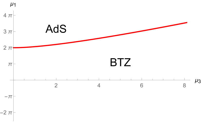
Figure 1: The phase-diagram on $\mu_{3}$-$\mu_{1}$ plane with $\mu_{3}\geq 0$. (Euclidean) BTZ is the leading contribution to the generalized partition function (91) in the region below the red curve. In particular, BTZ is always the leading saddle for non-positive $\mu_{1}$.

It is important to point out that the condition $f>0$ is necessary only to ensure positivity of temperature $T>0$. As a geometry in Lorentzian signature (66,67) is well-defined and smooth also for negative $f$ as long as the condition (74) is satisfied. For one-cut $u(\varphi)$ and $f$ given by (88) the condition (74) can be satisfied provided $f$ and $T$ are negative. Hence we arrive at an unusual situation when ${\mathcal{H}}=\mu_{1}Q_{1}+\mu_{3}Q_{3}$ may have a static solitonic solution which nevertheless does not correspond to a saddle point configuration upon analytic continuation to Euclidean signature. This is because the Euclidean geometry is a saddle point for a theory with the Hamiltonian $-{\mathcal{H}}$, which, in our case, would be unbounded from below.

7 Dominance of multi-cut solutions

The logic of this subsection is opposite to the previous one. We start with a particular one-cut solution $u(\varphi)$ characterized by some fixed $k,s_{1},q$, and make sure that corresponding geometry are smooth. We also find a Hamiltonian of the form ${\mathcal{H}}=\mu_{1}Q_{1}+\mu_{3}Q_{3}+\mu_{5}Q_{5}$, $\mu_{5}>0$, such that the black hole geometry build with this $u(\varphi)$ has a smaller free energy than any $u={\rm constant}$, i.e. thermal AdS or BTZ configuration.

We first find all ${\mathcal{H}}=\mu_{1}Q_{1}+\mu_{3}Q_{3}+\mu_{5}Q_{5}$ such that given $u(\varphi)$ is a static solution. For a solution of (40) the stabilizer vector field $f$ such that $\mathcal{D}f=0$ is always proportional to $f\propto u-s_{1}$. Any $Q_{2k+1}$ acting on a one-cut solution generates a flow proportional to $\partial_{\varphi}$, for example

$${c\over 24}\{Q_{5},u\}=(2s_{1}^{2}-s_{2})u^{\prime}.$$ (92)

Here and below $u_{i}$ and $s_{2},s_{3}$ are understood as functions of $k,s_{1},q$, given by (42-46). Therefore $\{{\mathcal{H}},u\}=0$ for ${\mathcal{H}}=\mu_{1}Q_{1}+\mu_{3}Q_{3}+\mu_{5}Q_{5}$ as long as

$$\mu_{1}+2s_{1}\mu_{3}+(2s_{1}^{2}-s_{2})\mu_{5}=0.$$ (93)

Equation (93) can be used to express $\mu_{1}$ in terms of $\mu_{3},\mu_{5}$. An overall rescaling of $\mu_{i}$ must be fixed by the requirement $T=1$. From the definition $f=2\pi{\delta H\over\delta u}$ we find

$$f=2(\mu_{3}+\mu_{5}\,s_{1})(u-s_{1}).$$ (94)

As discussed in the previous subsection, since $u$ oscillates between $u_{1}$ and $u_{2}$, the combination $u-s_{1}$ should be negative in order to have $\lambda_{0}>0$. For $T>0$ we therefore must require $\mu_{3}+\mu_{5}\,s_{1}<0$ such that $f$ is positive. Using (77) for one-cut solution we readily find

$$T=-(\mu_{5}s_{1}+\mu_{3}){\sqrt{2(s_{1}s_{2}-s_{3})}\over 2\pi}=1.$$ (95)

This fixes $\mu_{3}$ in terms of $\mu_{5}$. Hence for any given one-cut solution specified by $k,s_{1},q$ we have a family of Hamiltonians parametrized by $\mu_{5}$ such that $\{{\mathcal{H}},u\}=0$ and $T=1$, while $\mu_{1},\mu_{3}$ is fixed in terms of $\mu_{5}$ by (93) and (95).

Now we consider the smoothness condition (74), which is independent of the overall rescaling of $f$ and can be rewritten as $uf^{2}-ff^{\prime\prime}>0$. Taking into account that $u-s_{1}$ must be negative, this yields

$$(u-s_{1})^{2}-s_{1}^{2}-s_{2}<0.$$ (96)

Since $u_{1}\leq u\leq u_{2}$ and $u-s_{1}<0$, in the condition above we can take $u=u_{2}$, thus reducing it to a quadratic inequality on $s_{1}/k^{2}$. Together with the linear inequality $u_{1}+u_{2}>0$, which is equivalent to $u_{0}>0$, this becomes

$$\left\{\begin{array}[]{l}4s_{1}^{2}-4k^{2}\left(\theta_{2}(0;q)^{4}+\theta_{3}(0;q)^{4}\right)s_{1}-k^{4}(7\theta_{2}(0;q)^{8}+7\theta_{3}(0;q)^{8}+\theta_{4}(0;q)^{8})>0\\ s_{1}>k^{2}\left(\theta_{3}(0;q)^{4}+\theta_{4}(0;q)^{4}\right)\geq 2k^{2}.\end{array}\right.$$ (99)

The allowed region of $s_{1}/k^{2}$ as a function of $q$ is shown in Fig. 2. An additional analysis shows that in this region $\mu_{1},\mu_{5}>0$ and $\mu_{3}<0$, see Appendix A.

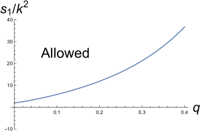
Figure 2: The allowed region of $s_{1}/k^{2}$ and $q$ satisfying both (99). The region above the blue curve is allowed. Thus, at least, $s_{1}$ should be greater than $2k^{2}$.

It is easy to see that second condition in (99), which is $u_{0}>0$, is not implying first condition, which is a consequence of (74). Hence, positivity of $u_{0}$ is necessary but not sufficient for the geometry to be regular.

Free energy of one-cut solution is given by

$$\mathcal{F}_{\text{1-cut}}(\mu_{5})=\frac{c}{12}(\mu_{1}Q_{1}+\mu_{3}Q_{3}+\mu_{5}Q_{5})-\frac{\pi c}{3}\sqrt{u_{0}},$$ (100)

where $u_{0}$ is given by (19) and $f$ is given by (94). The value of the charges $Q_{1},Q_{3},Q_{5}$ for the one-cut solution are given in (47) and (48). Thus, for a given one-cut solution with fixed $k,s_{1},q$, free energy $\mathcal{F}_{\text{1-cut}}$ is a function of $\mu_{5}$, while $\mu_{1}$ and $\mu_{3}$ are fixed by (93) and (95).

We want to compare free energy $\mathcal{F}_{\text{1-cut}}$ with those of thermal AdS, and BTZ solutions corresponding to ${\mathcal{H}}(\mu_{i})$ with the same values of chemical potentials and $T=1$. Free energy of thermal AdS is given by

$$\mathcal{F}_{\mathrm{AdS}}(\mu_{5}) =\frac{c}{12}(-\mu_{1}+\mu_{3}-\mu_{5})=-\frac{c}{12}\left((s_{1}+s_{2}+1)\mu_{5}+\frac{2\pi(2s_{1}+1)}{\sqrt{2(s_{1}s_{2}-s_{3})}}\right).$$ (101)

To BTZ solutions $u=u_{0}$ with temperature $T=1$ must satisfy

$$1=T=\frac{\mu_{1}+2\mu_{3}u_{0}+3\mu_{5}u_{0}^{2}}{2\pi}\sqrt{u_{0}}.$$ (102)

Since $\mu_{5}>0,\mu_{3}<0,\mu_{1}>0$, there are at most three solutions. We choose $u_{0}$ such that the free energy

$$\mathcal{F}_{\mathrm{BTZ}}(\mu_{5})=\frac{c}{12}(\mu_{1}u_{0}+\mu_{3}u_{0}^{2}+\mu_{5}u_{0}^{3})-\frac{\pi c}{3}\sqrt{u_{0}}$$ (103)

is smallest.

We plot free energies for one-cut, thermal AdS, and “smallest” BTZ solutions for some $k,s_{1},q$ as a function of $\mu_{5}$ in Fig. 3.

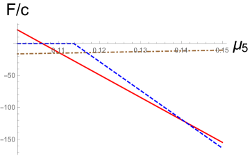
Figure 3: Free energy of the one-cut, “smallest” BTZ, and thermal AdS configurations as a function of $\mu_{5}$ for $k=1,s_{1}=38,q=0.6$. The solid red, dashed blue and dotted brown lines represent $\mathcal{F}_{\text{1-cut}}/c$, $\min\mathcal{F}_{\mathrm{BTZ}}/c$, and $\mathcal{F}_{\mathrm{AdS}}/c$ respectively. There is a region of $\mu_{5}$ where free energy $\mathcal{F}_{\text{1-cut}}$ (solid red line) is smaller than the two others.

There is clearly a region in the parameter space such that the one-cut solution has the smallest free energy among the considered configurations. Whether it is the leading saddle in this case remains unclear because the Hamiltonian in question also has two-cuts static solutions.

8 Discussion

In this paper we have constructed black hole geometries in AdS₃ which carry charges under the KdV symmetries. These geometries are static solutions in the theory of pure gravity in AdS₃ with the deformed boundary conditions, such that the Hamiltonian in the dual CFT is a linear combination of qKdV charges. Each geometry is specified by $u(\varphi)$ which is a static solution of a higher KdV equation, i.e. a finite zone Novikov solution when there are only finite number of KdV charges involved. Accordingly many properties of the black holes, including the first law of thermodynamics, follow directly from the geometry of the co-adjoint orbit of Virasoro algebra and basic properties of the KdV equations. Nevertheless there are several key ingredients which come from the bulk and are external to the classical KdV theory. First, this is the Bekenstein-Hawking entropy (76). Second, smoothness of the geometry in the bulk yields the regularity condition (74), which goes beyond the condition expected on the grounds that the new geometries are diffeomorphic to BTZ ones, namely that $u(\varphi)$ belongs to the Virasoro co-adjoint orbit ${\rm diff}\,\mathbb{S}^{1}/\mathbb{S}^{1}$ with $u_{0}>0$. It would be interesting to understand what this new condition means in terms of the finite zone solutions. Finally, thermodynamic identity requires $T>0$ and hence $f>0$. While this is not a condition on $u(\varphi)$, this is a condition on the pair ${\mathcal{H}}$ and $u$. More generally, the main questions formulated in this paper, of identifying $u$ which is the leading saddle for a given ${\mathcal{H}}$, and the question of identifying ${\mathcal{H}}$ such that given $u$ is its leading saddle, are the well posed new questions in the context of KdV theory.

The holographic dual of the classical GGE state discussed in this paper is the KdV analog of the GGE for another classical integrable model recently discussed in spohn2019generalized ; bulchandani1905gge . The next logical step here would be to develop a theory of generalized hydrodynamics describing long-wave dynamics of states locally deviating from the GGE castro2016emergent ; ilievski2017ballistic ; piroli2017transport ; bastianello2018generalized ; doyon2019generalized . This description should be valid both in the classical limit of field theory, and in the bulk, where it would describe the dynamics near a black hole background. In this context it would be interesting to see if the entropy (76) can be given a microscopic interpretation in terms of the classical field theory of $u(\varphi,t)$, providing geometric interpretation to black hole microstates.

The Euclidean black hole geometries are the classical saddles of the “generalized” Alekseev–Shatashvili path integral alekseev1989path decorated by higher KdV charges. A natural question would be to quantize small fluctuations around the black hole background to obtain $1/c$ corrections. This was done in GGE2 on the filed theory side for the conventional BTZ background, but the case of a non-constant $u(\varphi)$ needs to be treated separately. On a different note, in the limit of large temperature the boundary torus will reduce to a circle, while the Alekseev–Shatashvili path integral should reduce to the Schwarzian theory of SYK/JT gravity maldacena2016remarks ; stanford2017fermionic ; callebaut2019entanglement . It would be interesting to see if the geometries discussed in this paper would give rise to non-trivial saddle point configurations of the generalized Schwarzian theory which includes higher order operators, in particular $T\bar{T}$ deformation.

Appendix A Appendix: Signs of $\mu_{1}$, $\mu_{3}$ in the allowed region

In this appendix we show that $\mu_{1}>0$ and $\mu_{3}<0$ in the region specified by the smoothness condition (99). First, $\mu_{3}<0$ which simply follows from $\mu_{3}+\mu_{5}s_{1}<0$, see (95), and $s_{1}>2k^{2}$ imposed by (99).

Next, using (93) we find

$$\mu_{1}=\mu_{5}s_{2}-2s_{1}(\mu_{3}+\mu_{5}s_{1}).$$ (104)

Since $\mu_{5}>0$ and $\mu_{3}+\mu_{5}s_{1}<0$, we find $\mu_{1}>0$ if $s_{2}\geq 0$. Note that $s_{2}$ is given by (45) and it is a monotonically increasing function of $s_{1}>0$ for a fixed $q$. We check that $s_{2}$ as a function of $q$ for $s_{1}$ saturating the first constraint of (99) is positive as shown in Fig 4. Thus, $s_{2}\geq 0$ in the entire region where the inequalities (99) are satisfied. We therefore have $\mu_{1}>0$.

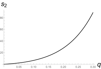
Figure 4: Plot of $s_{2}$ as a function of $q$ for $s_{1}(q)$ which saturates the first constraint of (99), i.e. along the blue curve in Fig. 2. For all $q>0$, $s_{2}$ is positive, and $s_{2}=0$ only for $q=0$. It means that $s_{2}\geq 0$ in the allowed region in Fig. 2.

- (1) P. Calabrese and J. Cardy, Time dependence of correlation functions following a quantum quench, Physical review letters 96 (2006) 136801.
- (2) P. Calabrese and J. Cardy, Quantum quenches in extended systems, Journal of Statistical Mechanics: Theory and Experiment 2007 (2007) P06008.
- (3) D. A. Roberts and D. Stanford, Two-dimensional conformal field theory and the butterfly effect, Phys. Rev. Lett. 115 (2015) 131603 [1412.5123].
- (4) V. V. Bazhanov, S. L. Lukyanov and A. B. Zamolodchikov, Integrable structure of conformal field theory, quantum kdv theory and thermodynamic bethe ansatz, Communications in Mathematical Physics 177 (1996) 381.
- (5) V. V. Bazhanov, S. L. Lukyanov and A. B. Zamolodchikov, Integrable structure of conformal field theory ii. q-operator and ddv equation, Communications in Mathematical Physics 190 (1997) 247.
- (6) V. V. Bazhanov, S. L. Lukyanov and A. B. Zamolodchikov, Integrable structure of conformal field theory iii. the yang–baxter relation, Communications in mathematical physics 200 (1999) 297.
- (7) V. V. Bazhanov, S. L. Lukyanov and A. B. Zamolodchikov, Quantum field theories in finite volume: Excited state energies, Nuclear Physics B 489 (1997) .
- (8) A. Maloney, G. S. Ng, S. F. Ross and I. Tsiares, Thermal correlation functions of kdv charges in 2d cft, Journal of High Energy Physics 2019 (2019) .
- (9) G. A. Kotousov and S. L. Lukyanov, Spectrum of the reflection operators in different integrable structures, 1910.05947.
- (10) B. Le Floch and M. Mezei, KdV charges in theories and new models with super-Hagedorn behavior, SciPost Phys. 7 (2019) 043 [1907.02516].
- (11) L. Vidmar and M. Rigol, Generalized gibbs ensemble in integrable lattice models, Journal of Statistical Mechanics: Theory and Experiment 2016 (2016) 064007.
- (12) J. Cardy, Quantum quenches to a critical point in one dimension: some further results, Journal of Statistical Mechanics: Theory and Experiment 2016 (2016) 023103.
- (13) J. de Boer and D. Engelhardt, Remarks on thermalization in 2d cft, Physical Review D 94 (2016) 126019.
- (14) A. Maloney, G. S. Ng, S. F. Ross and I. Tsiares, Generalized gibbs ensemble and the statistics of kdv charges in 2d cft, Journal of High Energy Physics 2019 (2019) .
- (15) A. Dymarsky and K. Pavlenko, Generalized gibbs ensemble of 2d cfts at large central charge in the thermodynamic limit, Journal of High Energy Physics 2019 (2019) 98.
- (16) A. Dymarsky and K. Pavlenko, Exact generalized partition function of 2d cfts at large central charge, Journal of High Energy Physics 2019 (2019) 77.
- (17) E. Witten, Coadjoint Orbits of the Virasoro Group, Commun. Math. Phys. 114 (1988) 1.
- (18) S. P. Novikov, The periodic problem for the korteweg–de vries equation, Funktsional’nyi Analiz i ego Prilozheniya 8 (1974) 54.
- (19) V. F. Lazutkin and T. Pankratova, Normal forms and versal deformations for hill’s equation, Functional Analysis and its applications 9 (1975) 306.
- (20) B. A. Dubrovin and S. P. Novikov, A periodicity problem for the korteweg–de vries and sturm–liouville equations. their connection with algebraic geometry, in Dokl. Akad. Nauk SSSR, vol. 219, pp. 531–534, 1974.
- (21) S. Novikov, S. Manakov, L. Pitaevskii and V. E. Zakharov, Theory of solitons: the inverse scattering method. Springer Science & Business Media, 1984.
- (22) F. Magri, A simple model of the integrable hamiltonian equation, Journal of Mathematical Physics 19 (1978) 1156.
- (23) J.-L. Gervais and A. Neveu, Dual string spectrum in polyakov’s quantization (ii). mode separation, Nuclear Physics B 209 (1982) 125.
- (24) I. M. Gel’fand and L. A. Dikii, Asymptotic behaviour of the resolvent of sturm-liouville equations and the algebra of the korteweg-de vries equations, Russian Mathematical Surveys 30 (1975) 77.
- (25) J.-L. Gervais, Infinite family of polynomial functions of the virasoro generators with vanishing poisson brackets, Physics Letters B 160 (1985) 277.
- (26) J.-L. Gervais, Transport matrices associated with the virasoro algebra, Physics Letters B 160 (1985) 279.
- (27) A. Dymarsky, K. Pavlenko and D. Solovyev, Zero modes of local operators in 2d cft on a cylinder, arXiv preprint arXiv:1912.13444 (2019) .
- (28) A. Pérez, D. Tempo and R. Troncoso, Boundary conditions for general relativity on ads3 and the kdv hierarchy, Journal of High Energy Physics 2016 (2016) 103.
- (29) O. Fuentealba, J. Matulich, A. Pérez, M. Pino, P. Rodríguez, D. Tempo et al., Integrable systems with bms poisson structure and the dynamics of locally flat spacetimes, JHEP 01 (2018) 148 [1711.02646].
- (30) E. Ojeda and A. Pérez, Boundary conditions for general relativity in three-dimensional spacetimes, integrable systems and the kdv/mkdv hierarchies, JHEP 08 (2019) 079 [1906.11226].
- (31) J. D. Brown and M. Henneaux, Central Charges in the Canonical Realization of Asymptotic Symmetries: An Example from Three-Dimensional Gravity, Commun. Math. Phys. 104 (1986) 207.
- (32) C. Bunster, M. Henneaux, A. Perez, D. Tempo and R. Troncoso, Generalized Black Holes in Three-dimensional Spacetime, JHEP 05 (2014) 031 [1404.3305].
- (33) M. Banados, C. Teitelboim and J. Zanelli, Black hole in three-dimensional spacetime, Physical Review Letters 69 (1992) 1849.
- (34) A. Dymarsky and K. Pavlenko, Generalized eigenstate thermalization hypothesis in 2d conformal field theories, Physical review letters 123 (2019) 111602.
- (35) S. Banerjee, J.-W. Brijan and G. Vos, On the universality of late-time correlators in semi-classical 2d CFTs, JHEP 08 (2018) 047 [1805.06464].
- (36) G. Vos, Vacuum block thermalization in semi-classical 2d CFT, JHEP 02 (2019) 022 [1810.03630].
- (37) C. Erices, M. Riquelme and P. Rodríguez, Btz black hole with korteweg–de vries-type boundary conditions: Thermodynamics revisited, Phys.Rev.D 100 (2019) 126026 [1907.13026].
- (38) H. Spohn, Generalized gibbs ensembles of the classical toda chain, Journal of Statistical Physics (2019) 1.
- (39) V. Bulchandani, X. Cao and H. Spohn, The gge averaged currents of the classical toda chain, arXiv preprint arXiv:1905.04548 .
- (40) O. A. Castro-Alvaredo, B. Doyon and T. Yoshimura, Emergent hydrodynamics in integrable quantum systems out of equilibrium, Physical Review X 6 (2016) 041065.
- (41) E. Ilievski and J. De Nardis, Ballistic transport in the one-dimensional hubbard model: The hydrodynamic approach, Physical Review B 96 (2017) 081118.
- (42) L. Piroli, J. De Nardis, M. Collura, B. Bertini and M. Fagotti, Transport in out-of-equilibrium xxz chains: Nonballistic behavior and correlation functions, Physical Review B 96 (2017) 115124.
- (43) A. Bastianello, B. Doyon, G. Watts and T. Yoshimura, Generalized hydrodynamics of classical integrable field theory: the sinh-gordon model, SciPost Phys 4 (2018) 33.
- (44) B. Doyon, Generalized hydrodynamics of the classical toda system, Journal of Mathematical Physics 60 (2019) 073302.
- (45) A. Alekseev and S. Shatashvili, Path integral quantization of the coadjoint orbits of the virasoro group and 2-d gravity, Nuclear Physics B 323 (1989) 719.
- (46) J. Maldacena and D. Stanford, Remarks on the sachdev-ye-kitaev model, Physical Review D 94 (2016) 106002.
- (47) D. Stanford and E. Witten, Fermionic localization of the schwarzian theory, Journal of High Energy Physics 2017 (2017) 8.
- (48) N. Callebaut and H. Verlinde, Entanglement dynamics in 2d cft with boundary: Entropic origin of jt gravity and schwarzian qm, Journal of High Energy Physics 2019 (2019) 45.