Thin-shell Wormholes with Ordinary Matter in Pure Gauss-Bonnet Gravity

Abstract

In this paper, we introduce higher dimensional thin-shell wormholes in pure Gauss-Bonnet gravity. The focus is on thin-shell wormholes constructed by $N\geq 5$-dimensional spherically symmetric vacuum solutions. The results suggest that, under certain conditions, it is possible to have thin-shell wormholes that both satisfy the weak energy condition and be stable against radial perturbations.

I Introduction

Wormholes and black holes are the most interesting solutions of the Einstein’s theory of gravity. While black holes are attractive for their simple structure and existence of the so-called event horizon, wormholes are rather mysterious for their geometrical and topological structures WH . Wormholes are hypothetical passages between two distinct and distant points within the same or different spacetimes. Traversable wormholes are even more interesting due to the opportunity they provide a traveler to make, in principle, impossible journeys possible WH . Due to the structure of a wormhole solution in $R$-gravity (general relativity), the corresponding energy-momentum tensor does not satisfy the necessary energy conditions WH , and hence, traversable wormholes are considered as “exotic” spacetimes. The major energy condition to determine the ordinariness of matter in wormhole literature is the weak energy condition (WEC). The WEC states $T_{\mu\nu}V^{\mu}V^{\nu}\geq 0$, in which $T_{\mu\nu}$ is the energy-momentum tensor and $V^{\mu}$ is an arbitrary timelike vector. In the context of perfect fluids, the WEC translates to two simultaneous conditions $\rho\geq 0$ and $\rho+p\geq 0$, where $\rho$ is the energy density and $p$ is the pressure. The latter condition alone is the null energy condition (NEC), which is clearly implied by the WEC. Since all known matters satisfy the WEC, we have given the name “exotic” to matters who do not. Believing in the nonexistence of exotic matters in our universe implies that traversable wormholes are not physical but some mathematical entities. Any attempt for finding wormhole solutions supported by ordinary matter in $R$-gravity has failed from the beginning. Hence, researchers moved on with modified theories of gravity such as $f\left(R\right)$ and Lovelock theories LWH .

On the other hand, an attempt by Visser to construct traversable wormholes using junction formalism brought some hope to the wormhole community since it minimized the amount of the exotic matter (in case they are not avoidable) TSW . Such wormholes have been called thin-shell wormholes (TSWs). Initially, TSW was proposed in Einstein’s $R$-gravity where two identical flat spacetimes with holes were glued together at the boundary of their holes. The common hole was indeed the throat of the constructed TSW and provided a passage between the two flat spacetimes TSW . Having finely chosen the geometry of the throat, gives the possibility to minimize the exotic matter which presents at the throat. The concept has been developed over the last three decades such that a rich literature on different aspects of TSWs are available TSWLit . Although TSWs are different from the former classic wormholes - due to the fact that they are not direct solutions to the Einstein field equation - they also suffer from the same obstacle as their former. This means that TSWs in $R$-gravity are supported by exotic matters, no matter what.

Moreover, TSWs may also suffer from instability against an external perturbation Stab . This is an important issue due to the application of TSWs. A traveler (or signal) who uses the throat, in general, makes interaction with the TSW which can be considered as a small or large perturbation. If such wormhole is not stable against the perturbation, it either collapses or evaporates. This is why, almost all constructed TSWs in the literature have been investigated for their stability, as well.

Here the question is “will constructing TSWs in modified theories of gravity give chances for having TSWs supported by ordinary matter?” The answer is yes TSWL1 ; TSWL2 ; TSWL3 ; TSWL4 ; TSWL5 ; TSWL6 and in the present study we shall give another evidence for a positive answer. In particular, in TSWL1 , authors study a TSW and its stability in $5$-dimensional Gauss–Bonnet (GB) gravity augmented by a Maxwell electromagnetic field, and find that the additional GB Lagrangian not only broadens the range of possible stable regions but also limits the amount of required exotic matter at the throat. Using the same gravity, authors show in TSWL2 that with fine-tuning the parameters, one could construct a TSW supported by ordinary matter, only when the GB parameter is negative. In TSWL3 , the radial stability of this TSW is investigated and it is shown that it is stable only for a very narrow region of fine-tuned parameters, again, only in case of a negative GB parameter. Another higher dimensional stable TSW with ordinary matter is studied in Einstein–Yang–Mills–Gauss–Bonnet gravity in TSWL4 . This TSW also exhibits the same behavior, in the sense that it is supported by ordinary matter only for negative values of GB parameter, and is stable against radial perturbation only for a narrow region on the stability diagram. In another attempt, authors construct a TSW in third-order Lovelock gravity in TSWL5 , and indicate that for a negative GB parameter and a positive third-order Lovelock parameter, the TSW could be sustained by ordinary matter. Yet, the stability diagrams show that for such TSW, the throat is radially stable only when the sound speed is negative throughout the matter. Finally, in TSWL6 , authors study the effect of the GB parameter in the stability of TSWs supported by a generalized Chaplygin gas and a general barotropic fluid, and conclude that although the GB parameter highly affects the stability regions in the diagrams, yet the corresponding TSWs does not satisfy the WEC. What distinguishes the present paper from its ancestors can be listed as follows: i) While in all previous studies an Einstein Lagrangian exists in the action, here we study pure GB which is free of the Einstein term. ii) In the mentioned studies above, a TSW could be supported by ordinary matter only when the GB parameter was negative. However, a negative GB parameter admits an exotic bulk spacetime where the associated solutions do not imply the classic limits of Schwarzschild or Reissner–Nordström solutions. On the other hand, in the present study the GB parameter has to be positive due to the nature of the solutions considered. iii) Unlike the previous studies, we do not limit our results by fine-tuning the parameters. The solution we are about to employ is chargeless, we consider no cosmological constant, and the GB parameter is positive-definite. Yet, we find TSWs with ordinary matter for a wide range of TSW radius. iv) We do not limit ourselves to a particular equation of state (EoS). The two EoSs we have used here are the barotropic EoS and the variable EoS Varela . While the former is the most used EoS in TSW literature, the latter is the most general EoS.

This terminology “pure Lovelock gravity” was used for the first time by Kastor and Mann Kastor1 and has been developed by Cai, et al. Cai1 , Dadhich, et al. PLT and others Others . The interesting fact about pure Lovelock gravity is that it admits non-degenerate vacua in even dimensions and unique non-degenerate dS and AdS vacua in odd dimensions Cai1 . Moreover, the corresponding black hole solutions are asymptotically indistinguishable from the ones in Einstein gravity PLT . This similar asymptotic behavior of two theories seems to extend also to the level of the dynamics and a number of physical degrees of freedom in the bulk PLT . The pure GB gravity that we consider here, is the second–order pure Lovelock gravity.

The paper is arranged as follows. In section II we briefly review the Lovelock and the pure Lovelock gravity and their solutions. In section III, within the standard framework of thin-shell formalism, we construct the TSW in the pure GB gravity for $N\geq 5$ dimensions, and investigate the conditions under which the TSW could be supported by ordinary matter. Section IV is devoted to the stability of the TSW against radial perturbation to see whether our ordinary-mattered TSW could be stable or not. Unfortunately, to the best of our knowledge, no method or formalism has been developed so far to study the stability of a TSW against an angular perturbation. Therefore, we only settle for a radial perturbation in this section. Finally, we bring our conclusion in section V. Throughout the paper, we have used the convention $G_{N}=c=1$.

II Pure Lovelock gravity: a review

Lovelock theory, is one of the higher dimensional modified theories of gravity which leaves the gravitational field equations second order Lovelock . The first order Lovelock theory is the Einstein $R$-gravity in all dimensions. The second order Lovelock theory is known as the Gauss-Bonnet (GB) theory and is defined for spacetimes with dimensions of five and higher. The third order Lovelock theory is applicable to seven dimensions and higher, and is well-known for the two additional coupling constants it provides. The general vacuum $N$-dimensional Lovelock theory is formulated with the action

$$I=\frac{1}{2\kappa_{N}}\int d^{N}x\sqrt{-g}\sum_{k=0}^{\left[\frac{N-1}{2}\right]}c_{k}\mathcal{L}_{k}$$ (1)

in which $\kappa_{N}$ is the Einstein’s constant in $N$ dimensions, $c_{k}$ are arbitrary real constants, $\left[\frac{N-1}{2}\right]$ is the integral part of $\frac{N-1}{2}$ and

$$\mathcal{L}_{k}=\frac{1}{2^{k}}\delta_{\mu_{1}\nu_{1}...\mu_{k}\nu_{k}}^{\alpha_{1}\beta_{1}...\alpha_{k}\beta_{k}}\prod\limits_{i=1}^{k}R_{\text{ \ \ \ \ \ \ \ }\alpha_{i}\beta_{i}}^{\mu_{i}\nu_{i}}$$ (2)

are the Euler densities of a $2k$-dimensional manifold, where the generalized Kronecker delta $\delta$ is defined as the anti-symmetric product

$$\delta_{\mu_{1}\nu_{1}...\mu_{k}\nu_{k}}^{\alpha_{1}\beta_{1}...\alpha_{k}\beta_{k}}=k!\delta_{[\mu_{1}}^{\alpha_{1}}\delta_{\nu_{1}}^{\beta_{1}}...\delta_{\mu_{k}}^{\alpha_{k}}\delta_{\nu_{k}]}^{\beta_{k}}.$$ (3)

For $k=0,$ we get $\mathcal{L}_{0}=1$ and $c_{0}$ will be the bare cosmological constant. For $k=1,$ one finds the Einstein-Hilbert Lagrangian where $\mathcal{L}_{1}=R$ and $c_{1}=1.$ The well known GB Lagrangian is found with $k=2$ such that

$$\mathcal{L}_{2}=\mathcal{L}_{GB}=R^{\kappa\lambda\mu\nu}R_{\kappa\lambda\mu\nu}-4R^{\mu\nu}R_{\mu\nu}+R^{2},$$ (4)

where $c_{2}$ is called the GB parameter. Finally, the third order Lovelock Lagrangian is given with $k=3$ where

$$\mathcal{L}_{3}=2R^{\kappa\lambda\rho\sigma}R_{\rho\sigma\mu\nu}R_{\hskip 8.5359pt\kappa\lambda}^{\mu\nu}+8R_{\hskip 8.5359pt\kappa\lambda}^{\mu\nu}R_{\hskip 8.5359pt\nu\rho}^{\kappa\sigma}R_{\hskip 8.5359pt\mu\sigma}^{\lambda\rho}+24R^{\kappa\lambda\mu\nu}R_{\mu\nu\lambda\rho}R_{\hskip 4.26773pt\kappa}^{\rho}+3RR^{\kappa\lambda\mu\nu}R_{\kappa\lambda\mu\nu}\\ +24R^{\kappa\lambda\mu\nu}R_{\mu\kappa}R_{\nu\lambda}+16R^{\mu\nu}R_{\nu\sigma}R_{\hskip 4.26773pt\mu}^{\sigma}-12RR^{\mu\nu}R_{\mu\nu}+R^{3},$$ (5)

and $c_{3}$ is the third order Lovelock parameter.

Considering an $N$-dimensional spherically symmetric static spacetime with line element

$$ds^{2}=-A\left(r\right)dt^{2}+\frac{dr^{2}}{A\left(r\right)}+r^{2}d\Omega_{N-2}^{2},$$ (6)

the Einstein-Lovelock’s field equation reduces to a $k$-order ordinary equation given by

$$\sum_{k=0}^{\left[\frac{N-1}{2}\right]}\tilde{c}_{k}\psi^{k}=\frac{\mu}{r^{N-1}},$$ (7)

in which $A\left(r\right)=1-r^{2}\psi\left(r\right)$, and the dimension-dependent mass parameter $\mu$ is related to the ADM mass $M$ of the (possible) asymptotically flat black hole or non-black hole solution by

$$\mu=\frac{2\kappa_{N}M}{\left(N-2\right)\Sigma_{N-2}}.$$ (8)

Furthermore,

$$\Sigma_{N-2}=\frac{2\pi^{\frac{N-1}{2}}}{\Gamma\left(\frac{N-1}{2}\right)}$$ (9)

is the surface area of the $\left(N-2\right)$-dimensional unit sphere, $\tilde{c}_{0}=\frac{c_{0}}{\left(N-1\right)\left(N-2\right)}$, $\tilde{c}_{1}=1$ and for $k\geq 2$

$$\tilde{c}_{k}=\prod\limits_{i=3}^{2k}\left(N-i\right)c_{k}.$$ (10)

In contrast to the general $m$-order Lovelock gravity with $1\leq m\leq\left[\frac{N-1}{2}\right]$, in $m$-order pure Lovelock gravity Kastor1 ; Cai1 ; PLT ; Others , except for $c_{0}$, all $c_{k}$ for $k\neq m$ are zero, while $c_{k=m}\neq 0.$ With the same line element as (6), the field equation of the $m$-order pure Lovelock gravity becomes

$$\tilde{c}_{0}+\tilde{c}_{m}\psi^{m}=\frac{\mu}{r^{N-1}}$$ (11)

where the general solution for $\psi$ is obtained to be

$$\psi\left(r\right)=\left\{\begin{array}[]{cc}\pm\left[\frac{1}{\tilde{c}_{m}}\left(\frac{1}{\ell^{2}}+\frac{\mu}{r^{N-1}}\right)\right]^{\frac{1}{m}},&m\text{ even}\\ \left[\frac{1}{\tilde{c}_{m}}\left(\frac{1}{\ell^{2}}+\frac{\mu}{r^{N-1}}\right)\right]^{\frac{1}{m}},&m\text{ odd}\end{array}\right.,$$ (12)

in which $\ell$ is the cosmological length in $\tilde{c}_{0}=-\frac{1}{\ell^{2}}.$ Finally, the metric function is given by

$$A\left(r\right)=\left\{\begin{array}[]{cc}1\mp r^{2}\left[\frac{1}{\tilde{c}_{m}}\left(\frac{1}{\ell^{2}}+\frac{\mu}{r^{N-1}}\right)\right]^{\frac{1}{m}},&m\text{ even}\\ 1-r^{2}\left[\frac{1}{\tilde{c}_{m}}\left(\frac{1}{\ell^{2}}+\frac{\mu}{r^{N-1}}\right)\right]^{\frac{1}{m}},&m\text{ odd}\end{array}\right..$$ (13)

In the rest of the paper we consider the pure GB gravity without the cosmological constant by setting $m=2$ and $c_{0}=0$ which result in

$$A\left(r\right)=1\mp\omega^{2}\,r^{\left(5-N\right)/2},$$ (14)

where $\omega^{2}\equiv\sqrt{\frac{\mu}{\tilde{c}_{2}}}$ is a positive constant. This solution for $N=5$ and $N>5$ admits different asymptotic behaviors. For $N=5$ the metric function in (14) reduces to

$$A\left(r\right)=1\mp\omega^{2},$$ (15)

constraint by $1\mp\sqrt{\frac{\mu}{\tilde{c}_{2}}}>0,$ which is an asymptotically non-flat spacetime and possesses a singularity at $r=0$ with a conical structure accompanied by a deficit (surplus) angle for the minus (plus) sign. For $N>5$ the asymptotically flat solution in (14) has a singularity at $r=0$, which is naked for the plus sign and is hidden behind an event horizon located at

$$r_{+}=\omega^{4/\left(N-5\right)}$$ (16)

for the minus sign.

III Thin-shell wormholes in pure GB gravity

To construct a TSW in an $N$-dimensional $m$-order pure Lovelock gravity, we excise out the inner part of a timelike hypersurface $\varSigma:=r-a=0$ in which $a>r_{h}$ ($r_{h}$ is the possible event horizon) and make two identical copies from the rest of the bulk spacetime (6), namely $\mathcal{M}^{\left(\pm\right)}.$ Afterwards, we glue the two incomplete manifolds $\mathcal{M}^{\left(\pm\right)}$ at their common boundary hypersurface $\varSigma.$ The resultant manifold, i.e. $\mathcal{M}=\mathcal{M}^{\left(+\right)}\cup\mathcal{M}^{\left(-\right)}$, is geodesically complete with a throat located at $r=a.$ Joining the two incomplete manifolds at $\varSigma$ requires the so-called generalized junction conditions to be satisfied. These conditions are, in summary, as follows. First of all, the induced metric tensor of the throat should be continuous across the shell i.e.,

$$\left[h_{ab}\right]_{-}^{+}=0$$ (17)

in which $\left[X\right]_{-}^{+}=\left(X\right)_{+}-\left(X\right)_{-}$ and $\left(h_{ab}\right)_{\pm}$ are the induced metric tensor at either sides of the throat defined by

$$\left(h_{ab}\right)_{\pm}\equiv\left(g_{\alpha\beta}\frac{\partial x^{\alpha}}{\partial\xi^{a}}\frac{\partial x^{\beta}}{\partial\xi^{b}}\right)_{\pm}.$$ (18)

Herein, $\left(x^{\alpha}\right)_{\pm}=\left\{t,r,\theta_{1},...,\theta_{N-2}\right\}_{\pm}$ are the coordinates of the bulk spacetime while $\left(\xi^{a}\right)_{\pm}=\left\{\tau,\theta_{1},...,\theta_{N-2}\right\}_{\pm}$ are the coordinates of the hypersurface with $\tau$ being the proper time. Upon satisfying the first junction condition, one finds $r_{\pm}=a\left(\tau\right),$ $\theta_{a\pm}=\theta_{a}$ and

$$\dot{t}_{\pm}^{2}=\frac{1}{A\left(a\right)}\left(1+\frac{\dot{a}^{2}}{A\left(a\right)}\right),$$ (19)

in which a dot stands for a derivative with respect to the proper time $\tau.$ Hence, the induced metric of the throat becomes

$$ds_{\varSigma}^{2}=-d\tau^{2}+a^{2}d\Omega_{N-2}^{2}.$$ (20)

The second junction condition implies that there is a discontinuity at the throat associated with the energy-momentum tensor of the fluid at the throat, given by the equation Davis

$$-\kappa_{N}S_{ab}=2c_{2}\left(3\left[J_{ab}\right]_{-}^{+}-h_{ab}\left[J\right]_{-}^{+}+2\left[\hat{P}_{amnb}K^{mn}\right]_{-}^{+}\right).$$ (21)

In (21), $S_{a}^{b}=diag\left[-\sigma,p,p,...,p\right]$ is the surface energy-momentum tensor,

$$\hat{P}_{amnb}=\hat{R}_{amnb}+\left(\hat{R}_{mn}h_{ab}-h_{an}\hat{R}_{mb}\right)-\left(\hat{R}_{an}h_{mb}-\hat{R}_{ab}h_{mn}\right)+\frac{1}{2}\hat{R}\left(h_{an}h_{mb}-h_{ab}h_{mn}\right)$$ (22)

is the divergence-free part of the Riemann tensor $\hat{R}_{amnb}$ (compatible with the metric of the induced metric),

$$J_{ab}=\frac{1}{3}\left(2KK_{am}K_{b}^{m}+K_{mn}K^{mn}K_{ab}-2K_{am}K^{mn}K_{nb}-K^{2}K_{ab}\right),$$ (23)

and $J=J_{a}^{a}$. Furthermore, in (23) $K_{ab}$ is the extrinsic curvature tensor (the second fundamental form) of the hypersurface defined by

$$\left(K_{ab}\right)_{\pm}=-\left(n_{\gamma}\right)_{\pm}\left(\frac{\partial^{2}x^{\gamma}}{\partial\xi^{a}\partial\xi^{b}}+\Gamma_{\alpha\beta}^{\gamma}\frac{\partial x^{\alpha}}{\partial\xi^{a}}\frac{\partial x^{\beta}}{\partial\xi^{b}}\right)_{\pm}$$ (24)

with the spacelike normal vector given by

$$\left(n_{\gamma}\right)_{\pm}=\pm\left(\frac{1}{\sqrt{g^{\alpha\beta}\frac{\partial\varSigma}{\partial x^{\alpha}}\frac{\partial\varSigma}{\partial x^{\beta}}}}\frac{\partial\varSigma}{\partial x^{\gamma}}\right)_{\pm}.$$ (25)

Using (21), one obtains the surface energy density and the lateral pressures as Mazhari

$$\sigma=-\frac{4\left(N-2\right)\tilde{c}_{2}}{3\kappa_{N}a^{3}}\sqrt{A+\dot{a}^{2}}\left(3-A+2\dot{a}^{2}\right)$$ (26)

and

$$p=\frac{4\tilde{c}_{2}}{3\kappa_{N}a^{2}\sqrt{A+\dot{a}^{2}}}\left[3\ddot{a}\left(1+A+2\dot{a}^{2}\right)+\frac{3}{2}A^{\prime}\left(1-A\right)+\frac{\left(N-5\right)}{a}\left(A+\dot{a}^{2}\right)\left(3-A+2\dot{a}^{2}\right)\right],$$ (27)

respectively. Note that, a dot stands for a derivative with respect to $\tau$ while a prime implies a derivative with respect to the radius $a$. By assuming a static equilibrium configuration for the throat, where $a=a_{0}$ and $\dot{a}=\ddot{a}=0$, the static surface energy density $\sigma_{0}$ and pressure $p_{0}$ are obtained as

$$\sigma_{0}=-\frac{4\left(N-2\right)\tilde{c}_{2}}{3\kappa_{N}a_{0}^{3}}\sqrt{A_{0}}\left(3-A_{0}\right)$$ (28)

and

$$p_{0}=\frac{4\tilde{c}_{2}}{3\kappa_{N}a_{0}^{2}\sqrt{A_{0}}}\left(\frac{3}{2}A_{0}^{\prime}\left(1-A_{0}\right)+\frac{\left(N-5\right)}{a_{0}}A_{0}\left(3-A_{0}\right)\right),$$ (29)

respectively, where $A_{0}=\left.A\left(r\right)\right|_{r=a_{0}}$ and $A_{0}^{\prime}=\left.dA\left(r\right)/dr\right|_{r=a_{0}}$. In what follows we shall study some specific cases regarding the dimensions and black hole/non-black hole spacetimes.

III.1 $N>5$-dimensional asymptotically flat bulk spacetime

As we have mentioned previously, for $N>5$ in the asymptotically flat solution (14), while the plus sign represents a non-black hole solution the minus sign admits a black hole. Inserting the static version of (14) into (28) and (29) one obtains

$$\sigma_{0}=-\frac{4\left(N-2\right)\tilde{c}_{2}}{3\kappa_{N}a_{0}^{3}}\sqrt{1\mp\omega^{2}\,a_{0}^{\left(5-N\right)/2}}\left(2\pm\omega^{2}\,a_{0}^{\left(5-N\right)/2}\right)$$ (30)

and

$$\sigma_{0}+p_{0}=\frac{4\tilde{c}_{2}}{\kappa_{N}a_{0}^{3}\sqrt{1\mp\omega^{2}\,a_{0}^{\left(5-N\right)/2}}}\left[\frac{N-1}{4}\left(\omega^{2}\,a_{0}^{\left(5-N\right)/2}\right)^{2}-2\pm\omega^{2}\,a_{0}^{\left(5-N\right)/2}\right],$$ (31)

where the upper (lower) sign is corresponding to the black hole (non-black hole) solution. For the lower sign, noting that $N>5$, we may have $\sigma_{0}\geq 0$ and $\sigma_{0}+p_{0}\geq 0$ only if

$$a_{0}\leq\left(\frac{\omega^{2}}{2}\right)^{2/\left(N-5\right)}=a_{c}.$$ (32)

Therefore, for any throat radius equal to or smaller than this critical radius $a_{c}$, a TSW constructed by an $N>5$-dimensional non-black hole spacetime solution to the pure GB gravity satisfies the WEC; consequently, the throat is indeed supported by ordinary matter rather than exotic. On the other hand, it is evident from (30) that the energy density for the black hole solution is negative-definite. Hence, a TSW constructed by such a spacetime is absolutely sustained by exotic matter.

III.2 $5$-dimensional conical bulk spacetime

In $5$-dimensional pure GB gravity, $A\left(a_{0}\right)=A_{0}\equiv 1\pm\omega^{2}$ is a positive constant, given by (15). The solution is singular at $r=0$ and admits deficit/surplus angle depending on whether $A_{0}$ is less or greater than unity, indicating the existence of a cosmic string. Following (28) and (29), one finds the surface energy density and lateral pressure at the throat by

$$\sigma_{0}=-\frac{4\tilde{c}_{2}}{\kappa_{N}a_{0}^{3}}\sqrt{A_{0}}\left(3-A_{0}\right)$$ (33)

and

$$p_{0}=0.$$ (34)

Since $A_{0}$ is positive, for any $A_{0}\geq 3$ we find $\sigma_{0}\geq 0$ and $\sigma_{0}+p_{0}\geq 0$. The matter at the throat satisfies the WEC and so is ordinary.

IV Stability analysis

To study the stability of the TSW in pure GB gravity, we start with the expression of $\sigma$ and $p$ given by Eqs. (26) and (27). From the energy conservation equation, i.e. $S_{;b}^{ab}=0$, one finds that the energy density in (26) and the pressure in (27) satisfy the relation

$$\frac{d\sigma}{da}+\frac{N-2}{a}\left(\sigma+p\right)=0.$$ (35)

In addition, Eq. (26) can be written in the form of a one-dimensional equation of motion for the radius of the throat as

$$\dot{a}^{2}+V\left(a\right)=0,$$ (36)

in which the first term is kinetic and the the second term is given by the effective potential

$$V\left(a\right)=A\left(a\right)-\left(\Psi\left(a\right)-\frac{1-A\left(a\right)}{2\Psi\left(a\right)}\right)^{2},$$ (37)

where

$$\Psi\left(a\right)=\left[\frac{\frac{16\left(N-2\right)\tilde{c}_{2}}{3\kappa_{N}a^{3}}}{\sqrt{\sigma^{2}+2\left(\frac{4\left(N-2\right)\tilde{c}_{2}}{3\kappa_{N}a^{3}}\right)^{2}\left(1-A\left(a\right)\right)^{3}}-\sigma}\right]^{1/3}.$$ (38)

After a radial perturbation is applied to the throat, its equation of motion becomes

$$\dot{a}^{2}+V\left(a\right)=v_{0}^{2},$$ (39)

in which $v_{0}$ is the initial velocity of the throat Zahra . For weak perturbation where $v_{0}^{2}\ll 1,$ one may expand the potential $V\left(a\right)$ near the equilibrium radius to write

$$\dot{x}^{2}+V\left(a_{0}\right)+V^{\prime}\left(a_{0}\right)u+\frac{1}{2}V^{\prime\prime}\left(a_{0}\right)u^{2}+\mathcal{O}\left(u^{3}\right)\simeq v_{0}^{2},$$ (40)

in which $u=a-a_{0}.$ Explicit calculation shows that although $V\left(a_{0}\right)\neq 0$, yet $V^{\prime}\left(a_{0}\right)=0$, upon which (40) becomes

$$\dot{u}^{2}+\frac{1}{2}V^{\prime\prime}\left(a_{0}\right)u^{2}\simeq v_{0}^{2}-V\left(a_{0}\right).$$ (41)

Clearly, with $V^{\prime\prime}\left(a_{0}\right)>0$, $u$ will be confined between the roots of $v_{0}^{2}=V\left(a_{0}\right)$, an indication of the stability of the throat after the radial perturbation. The potential $V\left(a\right)$ is of the form $V\left(a,\sigma\left(a\right)\right)$, hence in finding $V^{\prime\prime}\left(a\right)$ one needs to know $\sigma^{\prime}\left(a\right)$ and $\sigma^{\prime\prime}\left(a\right).$ In (35), $\sigma^{\prime}\left(a\right)$ has been already found by using the energy conservation equation. To calculate $\sigma^{\prime\prime}\left(a\right)$, we start from $\sigma^{\prime}\left(a\right)$, and considering a variable equation of state (EoS) Varela for the matter at the throat ($p$ will be a generic function of $\sigma$ and $a$ such that $p=p\left(\sigma,a\right)$), we obtain

$$\sigma^{\prime\prime}=\frac{N-2}{a^{2}}\left(\sigma+p\right)\left[N-1+\left(N-2\right)\left(\frac{\partial p}{\partial\sigma}\right)\right]-\frac{N-2}{a}\left(\frac{\partial p}{\partial a}\right).$$ (42)

At the equilibrium point, after the perturbation, one finds

$$\sigma_{0}=-\frac{4\left(N-2\right)\tilde{c}_{2}}{3\kappa_{N}a_{0}^{3}}\sqrt{A_{0}+v_{0}^{2}}\left(3-A_{0}+2v_{0}^{2}\right),$$ (43)

$$p_{0}=\frac{4\tilde{c}_{2}}{3\kappa_{N}a_{0}^{2}\sqrt{A_{0}+v_{0}^{2}}}\left[\frac{3}{2}A_{0}^{\prime}\left(1-A_{0}\right)+\frac{\left(N-5\right)}{a_{0}}\left(A_{0}+v_{0}^{2}\right)\left(3-A_{0}+2v_{0}^{2}\right)\right],$$ (44)

$$\sigma_{0}^{\prime}=-\frac{N-2}{a_{0}}\left(\sigma_{0}+p_{0}\right),$$ (45)

and

$$\sigma_{0}^{\prime\prime}=\frac{N-2}{a_{0}^{2}}\left(\sigma_{0}+p_{0}\right)\left[N-1+\left(N-2\right)\beta_{0}^{2}\right]+\frac{N-2}{a}\gamma_{0},$$ (46)

in which we have defined $\beta_{0}^{2}\equiv\left.\frac{\partial p}{\partial\sigma}\right|_{a=a_{0}}$ and $\gamma_{0}\equiv\left.-\frac{\partial p}{\partial a}\right|_{a=a_{0}}$. The parameter $\beta_{0}$ is interpreted as the speed of sound within the matter field at the throat. In case we encounter ordinary matter, we shall have the condition $\beta_{0}^{2}$$\in\left(0,1\right)$ since the speed of light is taken as unity. For the non-black hole solution, we have set $V^{\prime\prime}\left(a_{0}\right)$ equal to zero and then plotted $\beta_{0}^{2}$ against the revearsed and rescaled equilibrium radius $x_{0}\equiv\omega^{2}a_{0}^{(5-N)/2}$ for four different dimensions in Figs. 1 and 2, where $\gamma_{0}=0$ and $\gamma_{0}=\left.-p_{0}^{\prime}\right|_{a=a_{D}}$, respectively. Firstly, changing the static equilibrium radius from $a_{0}$ to $x_{0}$ allows us to project the plots for different dimensions onto a single diagram. The critical radius is now $x_{c}=2$ for every dimension, according to (32). However, since $N>5$, the condition (32) now reads $x_{0}\geq x_{c}=2$. Therefore, in Figs. 1 and 2, the matter distributed at the throat is ordinary post-$x_{c}$. Secondly, it is known that the choice $\gamma_{0}=0$ evokes the well-known barotropic EoS, in which the pressure is merely a generic function of the energy density, i.e. $p=p\left(\sigma\right)$. Also, the choice $\gamma_{0}=\left.-p_{0}^{\prime}\right|_{a=a_{D}}$, in which $a_{D}$ is the radius of discontinuity, is picked up deliberately since it removes the discontinuity in the stability diagram of barotropic TSWs Forghani . Although the discontinuity radius in the case we are studying here happens to locate behind the critical radius at $x_{0}=2$, setting $\gamma_{0}=\left.-p_{0}^{\prime}\right|_{a=a_{D}}$ alters the behavior of the graph. In fact, we would like to see how it affects the stability diagram of the TSW, for curosity. The discontinuity radius is where $\sigma_{0}^{\prime}$ becomes null. The value of the rescaled discontinuity radius is calculated as

$$x_{D}=\frac{2\left(1+\sqrt{2N-1}\right)}{N-1}.$$ (47)

It is evident that the value of this radius for $N\geq 6$ always happens to be less the value of the critical radius at $2$.

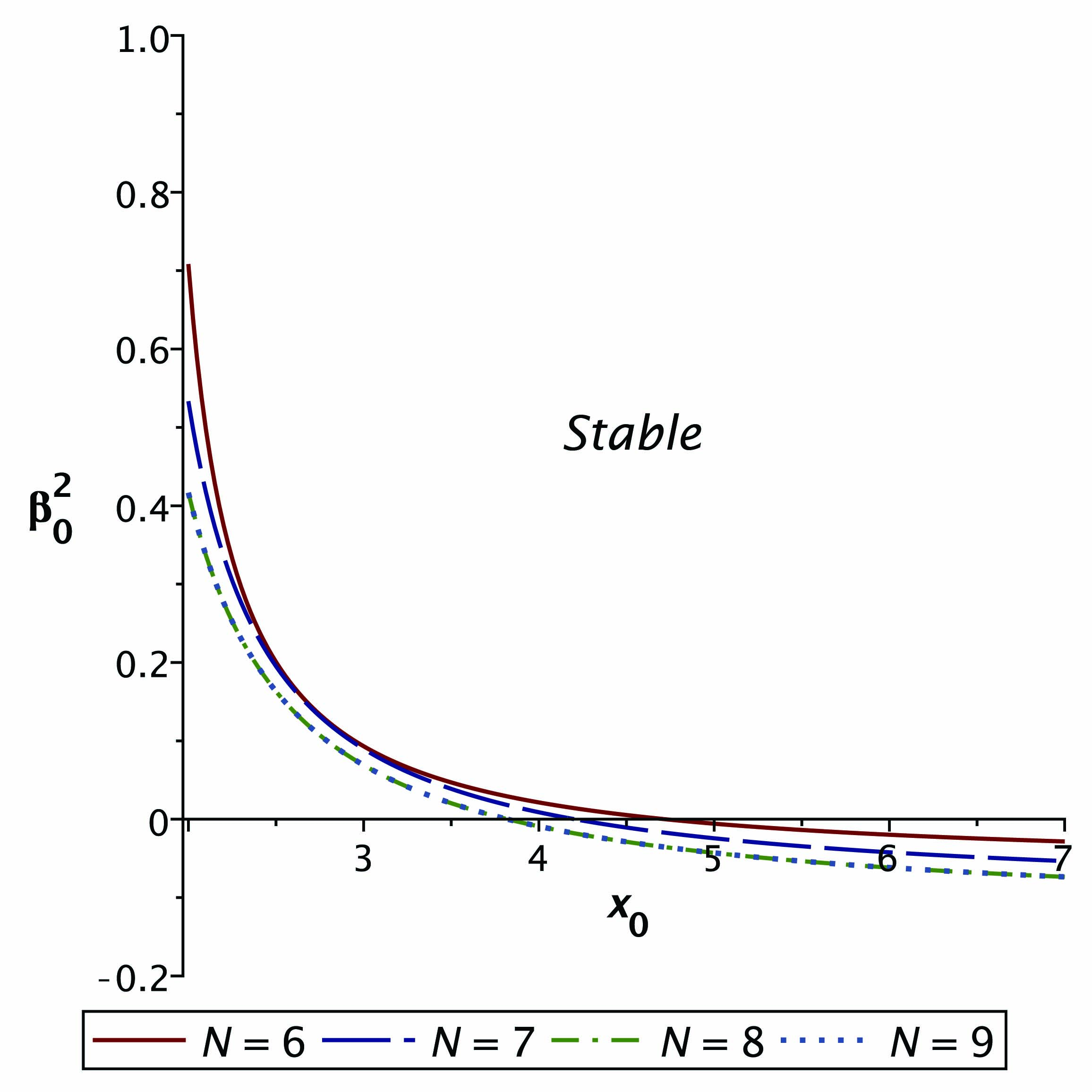
Figure 1: The stability diagrams for the non-black hole solution and a barotropic equation of state. The diagram plots $\beta_{0}^{2}$ against $x_{0}\equiv\omega^{2}a_{0}^{(5-N)/2}$ in four different dimensions. Note that the horizontal axis starts from the critical radius, beyond which the matter at the throat is ordinary.

In Figs. 1 and 2, the regions of stability, where $V^{\prime\prime}\left(a_{0}\right)$ is positive and the throat is at a stable equilibrium, are marked. As it can be perceived from Figs. 1 and 2, for both barotropic fluid and variable EoS fluid (and for the dimensions considered here), the TSW could be radially stable in the physically meaningful range $\beta_{0}^{2}\in\left(0,1\right)$ beyond the critical radius $x_{c}=2$. Therefore, a TSW constructed by a non-black hole vacuum solution in pure GB gravity, can maintain ordinary matter and is stable against radial perturbations either the fluid is supported by a barotropic or a variable EoS. Furthermore, it is evident that for higher dimensions, it is more likely for the TSW to be stable for both barotropic and variable EoSs. In addition, for counterpart number of dimensions, a variable EoS TSW is more likely to be stable than a barotropic TSW.

To complete our discussion in this part, let us argue the limit of the real radius of TSW $a_{0}$. The critical radius in (32) becomes

$$a_{c}=\left(\frac{\mu}{4\tilde{c}_{2}}\right)^{\frac{1}{N-5}},$$ (48)

according to our definition $\omega^{2}\equiv\sqrt{\frac{\mu}{\tilde{c}_{2}}}$. This critical radius, as the upper limit of the radius of the TSW, is comparable to the radius of the event horizon of a Schwarzschild-Tangherlini black hole in $N$ dimensions Tangherlini1

$$r_{ST}=\mu^{\frac{1}{N-3}},$$ (49)

and is not in quantum scale (Note that the modified GB parameter $\tilde{c}_{2}$ has dimension $L^{2}$).

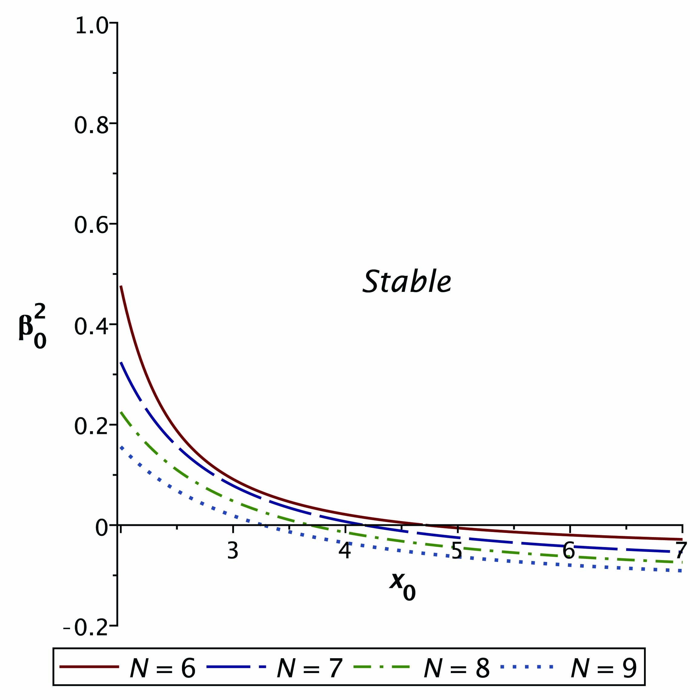
Figure 2: The stability diagrams for the non-black hole solution and a variable equation of state where $\gamma_{0}=\left.-p_{0}^{\prime}\right|_{a=a_{D}}$ is chosen for the explicit radial dependency of the pressure. The diagram plots $\beta_{0}^{2}$ against $x_{0}\equiv\omega^{2}a_{0}^{(5-N)/2}$ in four different dimensions. Note that the horizontal axis starts from the critical radius, beyond which the matter at the throat is ordinary.

For the cosmic string solution when $N=5$, our approach is slightly different. Fig. 3 directly displays $V^{\prime\prime}\left(a_{0}\right)/\beta_{0}^{2}$ against $a_{0}$, for four different values of $A_{0}$. The values of $A_{0}$ are chosen such that the TSW satisfies the WEC and the matter is ordinary. As can be observed, for all the values of $A_{0}>3$, $V^{\prime\prime}\left(a_{0}\right)/\beta_{0}^{2}$ is an absolutely positive function of $a_{0}$, which, considering the physical condition $\beta_{0}^{2}>0$, indicates that the TSW is stable against radial perturbations. The figure suggests that this stability is stronger for higher values of the constant $A_{0}$ and lower values of the radius of the throat $a_{0}$.

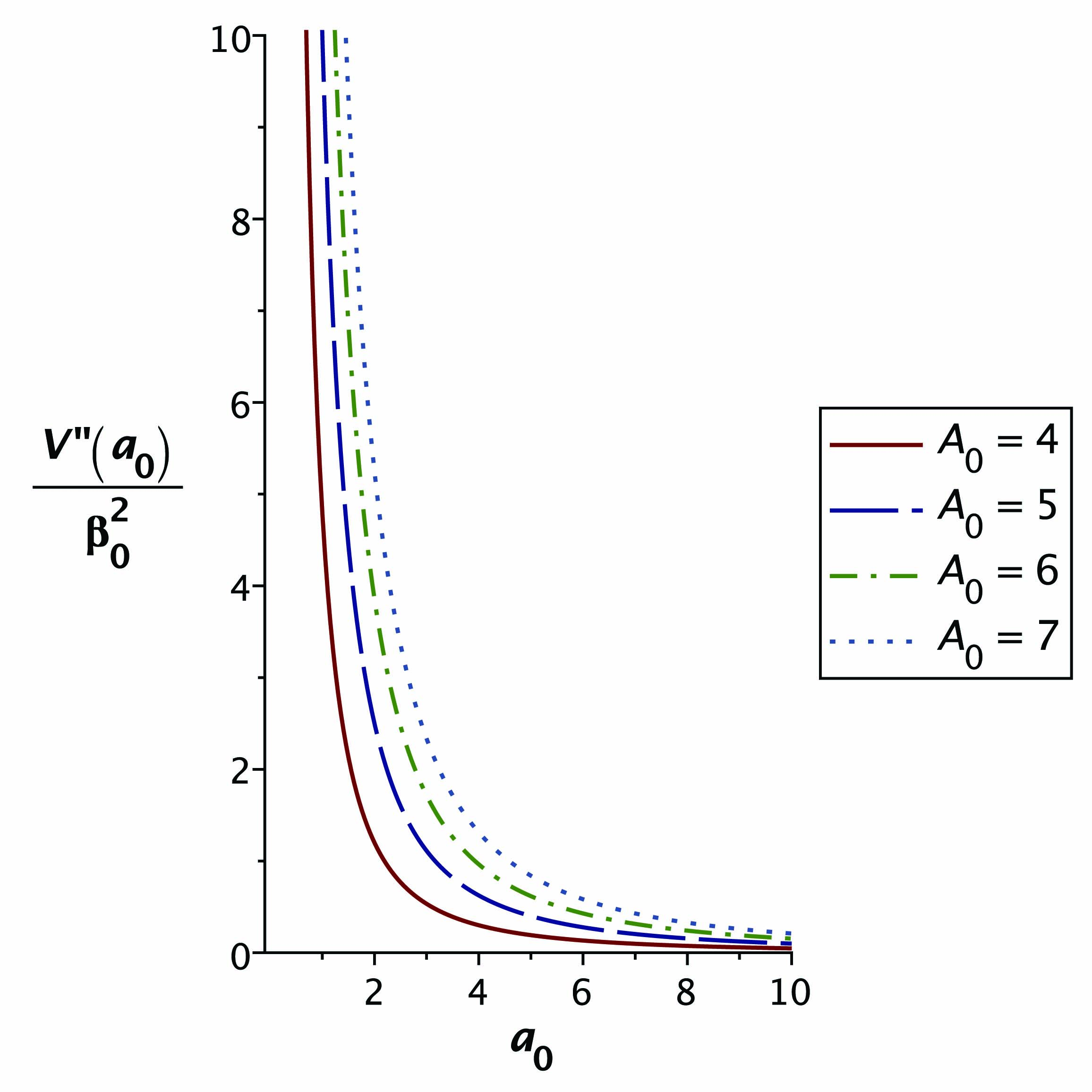
Figure 3: The plot indicates that $V^{\prime\prime}\left(a_{0}\right)/\beta_{0}^{2}$, for all the values of $A_{0}$ considered here, is positive for any radius of the throat.

V Conclusion

It has been decades that the cutting edge in wormhole studies has been to find a wormhole-like structure that satisfies the known energy conditions. It was known that in Einstein gravity, wormholes are supported by exotic matter, which does not satisfy the energy conditions. TSWs, which were introduced by Visser in 1989, opened doors to a wider class of wormhole-like structures which also had this advantage that the matter supported them was confined in a very limited area, say the throat of the TSW. However, it was soon learned that the TSWs suffer from the same exotic matter problem, as well. One way to bypass this problem is to rely on modified theories of gravity, towards which the Lovelock theory for its richness and simplicity is one of the best choices. TSWs in third order Lovelock gravity have been studied before and it was shown that under certain conditions they may satisfy the energy conditions Dehghani . In this study we challenged the pure Lovelock gravity of order two, i.e. the pure GB gravity. It was shown that for a non-black hole vacuum solution in $N>5$ dimensions, if the throat’s radius is less than a critical value (Eq. (32)), the thin-shell wormhole can be held together by ordinary matter. However, for a black-hole solution in $N>5$ dimensions, the energy density is always negative and hence the matter is always exotic. Also, it was demonstrated that for the vacuum cosmic string solution in $5$ dimensions, the matter is ordinary under some certain conditions ($A_{0}\geq 3$). In continuation, we investigated the stability of such TSWs under a radial perturbation by the standard linear stability analysis. It was observed from Figs. 1 and 2 that for the non-black hole TSW, there is a good possibility that the TSW is stable and physical either the ruling EoS is barotropic or variable. However, it is more likely for the TSW with a variable EoS to be stable than a TSW with a barotropic EoS. Moreover, Fig. 3 suggests that the cosmic string TSW is always stable when the matter is ordinary.

VI Abbreviations

• Equation of State

• Gauss–Bonnet

• Null Energy Condition

• Thin-Shell Wormhole

• Weak Energy Condition

VII Acknowledgment

SDF would like to thank the Department of Physics at Eastern Mediterranean University, especially the chairman of the department, Prof. İzzet Sakallı for the extended facilities.

References

- (1) M. S. Morris and K. S. Thorne, Am. J. Phys. 56, 395 (1988); M. S. Morris, K.S. Thorne and U. Yurtsever, Phys. Rev. Lett. 61, 1446 (1988); M. Visser, Lorentzian Wormholes - from Einstein to Hawking (American Institute of Physics, New York, 1995).
- (2) M. R. Mehdizadeh and F. S. N. Lobo, Phys. Rev. D 93, 124014 (2016); M. K. Zangeneh, F. S. N. Lobo and M. H. Dehghani, Phys. Rev. D 92, 124049 (2015); M. H. Dehghani and Z. Dayyani, Phys. Rev. D 79, 064010 (2009).
- (3) M. Visser, Phys. Rev. D 39, 3182 (1989); M. Visser, Nucl. Phys. B 328, 203 (1989).
- (4) E. Poisson and M. Visser, Phys. Rev. D 52, 7318 (1995); F. S. N. Lobo and P. Crawford, Class. Quantum Grav. 21, 391 (2004); E. F. Eiroa and C. Simeone, Phys. Rev. D 70, 044008 (2004); E. F. Eiroa and C. Simeone, Phys. Rev. D 81, 084022 (2010); F. S N Lobo and P. Crawford, Class. Quantum Grav. 22, 4869 (2005); N. M. Garcia, F. S. N. Lobo and M. Visser, Phys. Rev. D 86, 044026 (2012); E. F. Eiroa and C. Simeone, Phys. Rev. D 71, 127501 (2005); C. Bejarano and E. F. Eiroa, Phys. Rev. D 84, 064043 (2011); F. Rahaman, M. Kalam and S. Chakraborty, Gen. Relativ. Gravit., 38, 1687 (2006); E. F. Eiroa, M. G. Richarte and C. Simeone, Phys. Lett. A 373, 1 (2008); E. F. Eiroa and C. Simeone, Phys. Rev. D 82, 084039 (2010); M. Shrif and M. Azam, JCAP04(2013)023; M. Shrif and M. Azam, JCAP05(2013)025; X. Yue and S. Gao, Physics Letters A 375, 2193 (2011); M. G. Richarte and C. Simeone, Phys. Rev. D 80, 104033 (2009); S. H. Mazharimousavi, M. Halilsoy and Z. Amirabi, Phys. Lett. A 375, 3649 (2011); E. F. Eiroa and G. F. Aguirre, Eur. Phys. J. C 72, 2240 (2012); M. Sharif and M. Azam, Physics Letters A 378, 2737 (2014); F. Rahaman, P. K. F. Kuh ttig, M. Kalam, A. A. Usmani and S. Ray, Class. Quantum Grav. 28, 155021 (2011); A. C. Li et al., JCAP03(2019)016; S. D. Forghani, S. H. Mazharimousavi, and M. Halilsoy, JCAP10(2019)067.
- (5) E. Poisson and M. Visser, Phys. Rev. D 52, 7318 (1995).
- (6) M. Thibeault, C. Simeone and E. F. Eiroa, Gen. Relativ. Gravit., 38, 1593 (2006).
- (7) M. G. Richarte and Claudio Simeone, Phys. Rev. D 76, 087502 (2007); Erratum Phys. Rev. D 77, 089903 (2008).
- (8) S. H. Mazharimousavi, M. Halilsoy and Z. Amirabi, Phys. Rev. D 81, 104002 (2010).
- (9) S. H. Mazharimousavi, M. Halilsoy and Z Amirabi, Class. Quantum Grav., 28, 025004 (2011).
- (10) M. H. Dehghani and M. R. Mehdizadeh, Phys. Rev. D 85, 024024 (2012).
- (11) Z. Amirabi, M. Halilsoy and S. Habib Mazharimousavi, Phys. Rev. D 88, 124023 (2013).
- (12) V. Varela, Phys. Rev. D 92, 044002 (2015).
- (13) D. Kastor, and R. Mann, JHEP 04, 048 (2006).
- (14) R. G. Cai, and N. Ohta, Phys. Rev. D 74, 064001 (2006); R. G. Cai, L. M. Cao, Y. P. Hu, and S. P. Kim, Phys. Rev. D 78, 124012 (2008).
- (15) S. Chakraborty and N. Dadhich, Eur. Phys. J. C 78, 81 (2018); N. Dadhich and J. M. Pons, J. Math. Phys. 54, 102501 (2013); N. Dadhich, S. G. Ghosh and S. Jhingan, Phys. Rev. D 88, 084024 (2013); R. Gannouji and N. Dadhich, Class. Quantum Grav. 31, 165016 (2014); N. Dadhich and J. M. Pons, JHEP 05, 067 (2015); N. Dadhich, R. Durka, N. Merino and O. Miskovic, Phys. Rev. D 93, 064009 (2016); N. Dadhich, A. Molina and J. M. Pons, Phys. Rev. D 96, 084058 (2017); N. Dadhich, Eur. Phys. J. C 76, 104 (2016); X. O. Camanho and N. Dadhich, Eur. Phys. J. C 76, 149 (2016); N. Dadhich, S.G. Ghosh and S. Jhingan, Phy. Lett. B 711, 196 (2012);
- (16) J. M. Toledo and V. B. Bezerra, Gen. Relativ. Gravit. 51, 41 (2019); J. M. Toledoa and V. B. Bezerrab, Eur. Phys. J. C 79, 117 (2019); P. Concha and E. Rodríguez, Phys. Lett. B 774, 616 (2017); P. K. Concha, R. Durka, C. Inostroza, N. Merino and E. K. Rodríguez, Phys. Rev. D 94, 024055 (2016); B. Mirza, F. Oboudiat and S. Zare, Gen. Relativ. Gravit. 46, 1652 (2014).
- (17) D. Lovelock, J. Math. Phys. 12, 498 (1971).
- (18) S. C. Davis, Phys. Rev. D 67, 024030 (2003).
- (19) S. H. Mazharimousavi, M. Halilsoy and Z Amirabi, Class. Quantum Grav., 28, 025004 (2011); M. R. Mehdizadeh, M. Kord Zangeneh and F. S. N. Lobo, Phys. Rev. D 92, 044022 (2015).
- (20) Z. Amirabi, Eur. Phys. J. C 79, 410 (2019).
- (21) S. D. Forghani, S. H. Mazharimousavi, and M. Halilsoy, Eur. Phys. J. Plus 134, 342 (2019).
- (22) F. R. Tangherlini, IL NUOVO CIMENTO XXVII, 3 (1963); B. P. Singh, and S. G. Ghosh, Ann. Phys. (N. Y.) 395, 127–137 (2018).
- (23) M. H. Dehghani and M. R. Mehdizadeh, Phys. Rev. D 85, 024024 (2012); M. R. Mehdizadeh, M. Kord Zangeneh and F. S. N. Lobo, Phys. Rev. D 92, 044022 (2015).