Spectral and atmospheric characterisation of a new benchmark brown dwarf HD 13724 B

Abstract

Context. HD 13724 is a nearby solar-type star at 43.48 $\pm$ 0.06 pc hosting a long-period low-mass brown dwarf detected with the CORALIE echelle spectrograph as part of the historical CORALIE radial-velocity search for extra-solar planets. The companion has a minimum mass of $26.77^{+4.4}_{-2.2}\leavevmode\nobreak\ M_{\mathrm{Jup}}$ and an expected semi-major axis of $\sim$240 mas making it a suitable target for further characterisation with high-contrast imaging, in particular to measure its inclination, mass, and spectrum and thus establish its substellar nature.

Aims. Using high-contrast imaging with the SPHERE instrument on the Very Large Telescope (VLT), we are able to directly image a brown dwarf companion to HD 13724 and obtain a low-resolution spectrum.

Methods. We combine the radial-velocity measurements of CORALIE and HARPS taken over two decades and high-contrast imaging from SPHERE to obtain a dynamical mass estimate. From the SPHERE data we obtain a low-resolution spectrum of the companion from $Y$ to $J$ band, as well as photometric measurements from IRDIS in the $J$, $H,$ and $K$ bands.

Results. Using high-contrast imaging with the SPHERE instrument at the VLT, we report the first images of a brown dwarf companion orbiting the host star HD 13724. It has an angular separation of 175.6 $\pm$ 4.5 mas and an $H$-band contrast of $10.61\pm 0.16$ mag, and using the age estimate of the star to be $\sim$1 Gyr gives an isochronal mass estimate of $\sim$44 $M_{\mathrm{Jup}}$. By combining radial-velocity and imaging data we also obtain a dynamical mass of $50.5^{+3.3}_{-3.5}\leavevmode\nobreak\ M_{\mathrm{Jup}}$. Through fitting an atmospheric model, we estimate a surface gravity of $\log g=5.5$ and an effective temperature of 1000 K. A comparison of its spectrum with observed T dwarfs estimates a spectral type of T4 or T4.5, with a T4 object providing the best fit.

1 Introduction

Evolutionary models of brown dwarfs are plagued by a lack of observational constraints in addition to model degeneracies. The complex molecular chemistry of their atmospheres leaves a relatively wide parameter space for models to span. For this reason, the detection of brown dwarfs is vital to testing the complex atmospheres, structure, and evolution of these substellar objects (Baraffe et al., 2003, 2015). Furthermore, it is important to characterise brown dwarfs that are orbiting stars, where the age of the system can be constrained, unlike field brown dwarfs. In addition, brown dwarfs orbiting stars provide an opportunity to monitor the radial velocity (RV) of these systems which allows us to place constraints on their dynamical masses over time (Boden et al., 2006).

With over 20 years worth of RV measurements from the CORALIE survey for extrasolar planets (Udry et al., 2000), HD 13724 has been identified as a promising candidate for observational follow-up with direct imaging (Rickman et al., 2019) due to its minimum mass ($26.77^{+4.4}_{-2.2}M_{\mathrm{Jup}}$) and expected semi-major axis ($\sim$240 mas), which was calculated from the orbital period, itself derived from RV measurements.

The CORALIE RV survey is a volume-limited sample of 1647 main sequence stars from F8 down to K0 located within 50 pc of the Sun. Such a long base line of observations allows us to detect massive giant planets at separations of larger than 5 AU. This in turn identifies golden targets for direct imaging, as such companions are rare and are very difficult to search for blindly. Selecting long-period candidates to image from RV surveys has proven to be valuable (see Cheetham et al. (2018); Peretti et al. (2019)).

Radial-velocity measurements provide a lower limit on the measured masses due to the unknown orbital inclination. Therefore, directly imaging long-period RV candidates allows us to break that degeneracy and provide constraints on the dynamical mass of the companion.

Not only does combining these two detection techniques allow us to start filling in a largely unexplored parameters space, but through combining RV and direct imaging data we can now expect to dynamically measure the mass of such companions. By constraining the mass, we are able to place additional constraints on the evolution of the companion, both in terms of temperature and atmospheric composition (e.g. see Maire et al. (2016a); Vigan et al. (2016)).

To date, individual dynamical masses from combining radial velocity and imaging measurements are known for only a handful of brown dwarfs (Thalmann et al., 2009; Sahlmann et al., 2011; Crepp et al., 2012, 2014, 2016; Dupuy & Liu, 2017; Peretti et al., 2019; Bowler et al., 2018; Cheetham et al., 2018; Brandt et al., 2019; Maire et al., 2019), therefore any new detections contribute significantly to brown dwarf models in addition to providing important analogues for the characterisation of exoplanets. This forms part of a larger effort to determine the giant planet upper mass limit and lower mass limit for brown dwarfs, especially in the $\sim$20 $M_{\mathrm{Jup}}-$40 $M_{\mathrm{Jup}}$ range where there is a dearth of observed companions (Sahlmann et al., 2011). Detecting brown dwarfs in this parameter space can help us to understand the formation of these objects, whether they formed via gravitational instability like binary systems or via core-accretion, as in the case of planets. This is crucial to understanding the formation processes of such systems and to defining the boundary between massive planets and low-mass brown dwarfs.

To determine the mass of an imaged brown dwarf companion, the key parameter for the evolution of substellar objects, we usually rely on evolutionary models (Marley et al., 1996; Baraffe et al., 2003; Allard et al., 2012; Morley et al., 2012). These models still need to be tested and properly calibrated through observations and the discovery of benchmark sources provides a powerful and critical tool to achieve this. Furthermore, as we move toward imaging increasingly small objects it is important to use them to test theoretical atmospheric models.

Typically, the conditions around young stars are more favourable to direct imaging because any companion will still be bright and hot and therefore easier to detect. In contrast, the RV method is typically suited to older stars where the RV signal is not too contaminated from variability caused by stellar activity in young and active stars. Consequently, combining these two techniques allows us to not only probe a mass-separation parameter space that is largely unexplored, but also bridge the gap between younger and older companion candidates.

Here, we report the first images and low-resolution spectrum of the benchmark brown dwarf HD 13724 B. In addition, we extend the time baseline of the RV observations. When combined with the imaging data, this allows constraints to be placed on the mass and orbital parameters of the brown dwarf companion. Thanks to the high precision of the RV data and the number of points, the minimum mass is well constrained, meaning that only a few astrometric points from high-contrast imaging were necessary to ensure a high-precision orbit and dynamical mass.

The paper is organised as follows. The properties of the host star are summarised in Sect. 2. In Sect. 3 we summarise the observations and data analysis procedures for the RV and high-contrast imaging data. In Sect. 4 we present the results of the imaging data analysis and derived companion properties, and give an overview of the results from the combined orbital fitting. The results are discussed in Sect. 5 with some concluding remarks.

2 Stellar characterisation

The observed and inferred stellar parameters for HD 13724 are summarised in Table 1. The spectral type, V band magnitude, and colour index are taken from the HIPPARCOS and Tycho catalogues (Hoeg et al., 1997; Perryman et al., 1997), while the astrometric parallax ($\pi$) and luminosity are taken from the second Gaia data release (Gaia Collaboration et al., 2018). The effective temperature, gravity and metallicities were derived using the same spectroscopic methods as applied in Santos et al. (2013), whilst the $v\sin i$ is computed using the calibration of CORALIE’s Cross Correlation Function (CCF; Santos et al., 2001; Marmier, 2014).

The mean chromospheric activity index - $\log(R^{\prime}_{HK})$ - is computed by co-adding the corresponding CORALIE spectra to improve the signal-to-noise ratio which allows us to measure the Ca II re-emission at $\lambda=3933.66$ Å. We derived an estimate of the rotational period of the star from the mean $\log(R^{\prime}_{HK})$ activity index using the calibration of Mamajek & Hillenbrand (2008).

The stellar radius and uncertainties are derived from the Gaia luminosities and the effective temperatures are obtained from the spectroscopic analysis. A systematic error of 50 K was quadratically added to the effective temperature error bars and propagated in the radius uncertainties.

The mass and age of HD 13724, as well as the uncertainties, were derived using the Geneva stellar evolution modes (Ekström et al., 2012; Georgy et al., 2013). The interpolation in the model grid was made through a Bayesian formalism using observational Gaussian priors on $T_{\mathrm{eff}}$, $M_{V}$, $\log g,$ and [Fe/H] (Marmier, 2014).

Table 1: Stellar parameters of HD 13724

Parameters	units	HD 13724
Spectral type		G3/G5V
$V$		7.89
$B-V$		0.667
$\pi$	$[\text{mas}]$	23.0 $\pm$ 0.03
$M_{v}$		4.70
$T_{\mathrm{Gaia}}$	$[\text{K}]$	$5775.33^{+49.67}_{-74.33}$
$\log g$	$[\text{cgs}]$	4.44 $\pm$ 0.07
$[\text{Fe/H}]$	$[\text{dex}]$	0.23 $\pm$ 0.02
$v\sin i$	$[\text{km s}^{-1}]$	3.025
$M_{*}$	$[\text{M}_{\odot}]$	1.14 $\pm$ 0.06
$L_{\mathrm{Gaia}}$	$[L_{\odot}]$	$1.14^{+0.001}_{-0.002}$
$R_{\mathrm{Gaia}}$	$[R_{\odot}]$	1.07 $\pm$ 0.02
$\log R^{{}^{\prime}}_{HK}$		-4.76 $\pm$ 0.003
$P_{\text{rot}}$	$[\text{days}]$	20.2$\pm$1.2
Age	$[\text{Gyr}]$	1.04 $\pm$ 0.88

3 Observations and data reduction

Radial-velocity and direct imaging observations were combined to constrain the orbit of HD 13724 B. Furthermore, the extensive orbital coverage of the RV time series allows us to precisely constrain its orbital parameters. Combined with several direct imaging observations we are able to derive the orbital inclination $i$ and thus the mass. In addition, the SPHERE high-contrast IRDIS observations provide six narrow-band-width photometric measurements in the $J$, $H,$ and $K$ bands and IFS observations allow us to obtain a low-resolution spectrum of the brown dwarf companion in the $Y-J$ bands.

3.1 Radial velocities

HD 13724 has been observed since August 1999 with the CORALIE spectrograph (Queloz et al., 2000) installed on the 1.2m EULER Swiss telescope at La Silla observatory (Chile) and HARPS (Mayor et al., 2003) on the ESO/3.6 m telescope to obtain RVs.

The RV data analysis presented in this paper was accomplished using a set of online tools hosted by the Data and Analysis Center for Exoplanets (DACE) , which performs a Keplerian fit to the data as described in Delisle et al. (2016). The 179 measurements obtained between August 1999 and December 2019 are shown in Fig. 1 with the corresponding Keplerian model.

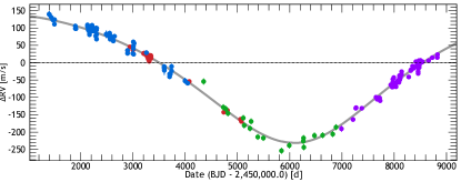
Figure 1: HD13724 RV measurements as a function of Julian Dates obtained with CORALIE-98 (blue), CORALIE-07 (green), and CORALIE-14 (purple). The HARPS-03 data are shown in red. The best single-planet Keplerian model is represented as a black curve.

Following on from Rickman et al. (2019) we obtained five more RV measurements over $\sim$10 months. We also added four historical and low-precision ($\sim$ 300 m/s) CORAVEL measurements to increase the overall time-span of the RV measurements by 10 years and to provide an upper bound constraint on the minimum mass of the companion. The RV data products presented in this paper are available at DACE with the new orbital parameters shown in Table 5. The full description of the RV data is outlined in Rickman et al. (2019).

3.2 SPHERE high-contrast imaging

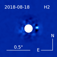
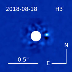
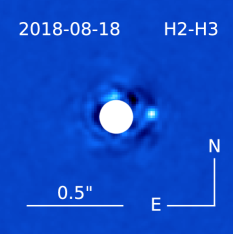
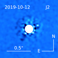
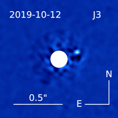
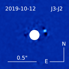
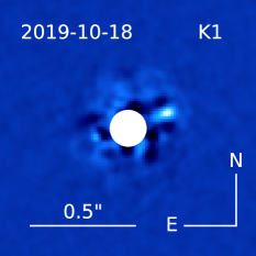
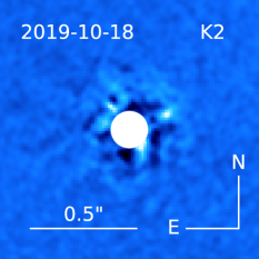
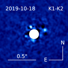
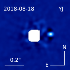
Figure 2: IRDIS and IFS images of HD 13724. The star is masked by the white circle. We also show a weighted combination of the IFS SDI image. Each IFS wavelength channel was weighted by the average flux predicted by the best-fitting BT-Settl model (Allard et al., 2012).

HD 13724 was observed with SPHERE, the extreme adaptive optics system at the VLT (Beuzit et al., 2019) on 18 Aug 2018, 12 Oct 2019, and 18 Oct 2019. Observations were taken using the IRDIFS mode, which allows the Integral Field Spectrograph (IFS; Mesa et al. (2015)) and the InfraRed Dual-Band Imager and Spectrograph (IRDIS; Dohlen et al. (2008)) modules to be used simultaneously. The IFS data cover a range of wavelengths from $Y-J$ (0.96-1.34$\mu$m, spectral resolution $R\sim 54$). The IRDIS data were taken in dual-band imaging mode (Vigan et al., 2010) using the $H2$ and $H3$ filters ($\lambda_{H2}=1.58888\mu$m, $\lambda_{H3}=1.6671\mu$m), as well as using the $J2$ and $J3$ filters ($\lambda_{J2}=1.190\mu$m, $\lambda_{J3}=1.273\mu$m) and the $K1$ and $K2$ band filters ($\lambda_{K1}=2.110\mu$m and $\lambda_{K2}=2.251\mu$m), such that the $J2$, $H3,$ and $K2$ bands align with methane absorption bands.

The observing sequence consisted of long-exposure images taken with an apodized Lyot coronagraph (Soummer et al., 2003). To measure the position of the star behind the coronograph, several exposures were taken with a sinusoidal modulation applied to the deformable mirror (to generate satellite spots around the star) at the beginning and at the end of the sequence. To estimate the stellar flux and the shape of the point-spread function (PSF) during the sequence, several short-exposure images were taken with the star moved from behind the coronograph, and using a neutral-density (ND) filter with a $\sim 10\%$ transmission, also at the beginning and end of the sequence. In addition, several long-exposure sky frames were taken to estimate the background flux and help identify bad pixels on the detector.

The SPHERE Data Reduction and Handling pipeline (Pavlov et al., 2008) was used to perform the wavelength extraction for the IFS data, turning the full-frame images of the lenslet spectra into image cubes. The remainder of the data reduction and analysis was completed using the Geneva Reduction and Analysis Pipeline for High-contrast Imaging of planetary Companions (GRAPHIC) (Hagelberg et al., 2016). The data were first sky subtracted, flat fielded, cleaned of bad pixels, and corrected for distortion (following Maire et al. (2016b)). We then ran a principal component analysis (PCA) PSF substraction algorithm (Soummer et al., 2012; Amara & Quanz, 2012) which is run separately for images at each wavelength channel and for each IRDIS channel. The resulting frames were derotated and median combined to produce a final PSF-substracted image.

In addition to this, we performed a spectral differential imaging (SDI) reduction for both the IFS and IRDIS datasets. The same PCA algorithm was then performed on the resulting images. The resulting PCA-reduced and SDI IRDIS and IFS images are shown in Fig. 2.

4 Results

4.1 Astrometry and photometry

The relative astrometry and photometry were calculated using a negative fake-planet injection on the images (Bonnefoy et al., 2011). An initial Nelder-Mead minimisation routine (Gao & Han, 2012) was used to find a first-order estimation of the separation (in pixels), position angle (in degrees), and contrast ratio between the star and the companion. We then fitted over a 3D grid of parameters for the position and the flux of the fake negative PSF to minimise the residuals and to numerically derive the $\chi^{2}$ with the associated 68.27% confidence interval. Subsequently, we corrected for the pixel scale and true north angle given in Maire et al. (2016b). The resulting parameters are listed in Table 4.

The IFS data were taken in the wavelength range 0.96-1.34$\mu$m which is split into 39 wavelength channels, giving 39 images across the wavelength range. Because of the low signal-to-noise ratio in some of the spectral channels, we used a different approach to measure the companion flux. For the IFS data, we performed a fit for the separation and position angle using the negative fake-planet injection using a stacked image across all of the wavelength channels in order to have a high signal-to-noise ratio for the companion fit. Using this fitted position on the image, we then fitted for the contrast ratio between the companion and the star at each wavelength channel in order to extract the spectrum.

Table 2: Measured relative astrometry and photometry of HD 13724 B from the SPHERE observations.

Instrument	Filter	Date	BJD	$\rho$ (mas)	$\theta$ (deg)	Contrast (mag)
IRDIS	H2	2018-08-18	58349.29438	175.61 $\pm$ 4.45	272.15 $\pm$ 1.06	10.61 $\pm$ 0.16
IRDIS	H3	2018-08-18	58349.29438	178.85 $\pm$ 4.56	272.50 $\pm$ 1.71	11.34 $\pm$ 0.32
IRDIS	H2-H3	2018-08-18	58349.29438	177.70 $\pm$ 4.41	270.75 $\pm$ 1.76	11.71 $\pm$ 0.35
IRDIS	J2	2019-10-12	58768.16564	179.9 $\pm$ 12.69	289.92 $\pm$ 2.49	11.50 $\pm$ 0.40
IRDIS	J3	2019-10-12	58768.16564	188.90 $\pm$ 4.98	288.75 $\pm$ 1.05	10.37 $\pm$ 0.04
IRDIS	J3-J2	2019-10-12	58768.16564	187.59 $\pm$ 1.60	288.25 $\pm$ 0.58	10.82 $\pm$ 0.09
IRDIS	K1	2019-10-18	58774.20206	190.55 $\pm$ 9.05	288.75 $\pm$ 1.51	10.29 $\pm$ 0.18
IRDIS	K2	2019-10-18	58774.20206	192.12 $\pm$ 15.84	288.75 $\pm$ 2.52	11.10 $\pm$ 0.46
IRDIS	K1-K2	2019-10-18	58774.20206	200.32 $\pm$ 16.15	288.58 $\pm$ 2.62	11.15 $\pm$ 0.43

4.2 Orbit determination and dynamical mass

To constrain the orbital parameters of the brown dwarf, we performed a combined fit to the RV and direct-imaging data. For this we used the IRDIS $H2$, $H3$, $J2$, $J3$, $K1$ and $K2$ astrometry $\{\rho(t),\theta(t)\}$ where $\rho(t)$ is the observed separation in mas and $\theta(t)$ is the position angle in degrees (see Table 4). This allows us to place constraints on the period, eccentricity, and inclination of the system.

Due to two major upgrades to CORALIE in June 2007 (Ségransan et al., 2010) and in November 2014, we consider CORALIE as three different instruments, corresponding to the different upgrades: the original CORALIE as CORALIE-98 (C98), the first upgrade as CORALIE-07 (C07), and the latest upgrade as CORALIE-14 (C14).

The observed RV signal was modelled with a single Keplerian and five RV offsets (corresponding to one offset for each RV instrument). HARPS-03 was chosen as the reference instrument while RV offsets were adjusted between CORAVEL, CORALIE-98, CORALIE-07, CORALIE-14, and HARPS-03; where each of the instrumental offsets were margnialised over for the fit.

A linear correlation is observed between the $H_{\alpha}$ activity index time series and the observed RVs which allows us to carry out a first-order detrending of the observed RV measurements using a linear scale factor between the $H_{\alpha}$ index time series and the modelled RVs (Delisle et al., 2018). A RV nuisance parameter – corresponding to the white noise component of the stellar activity – is added to the noise model of the likelihood function and is adjusted in the MCMC.

Regarding the Keplerian motion, we choose to adjust the natural log of the period and of the RV semi-amplitude to increase the efficiency of the MCMC due to the partial coverage of the orbit. We also probe the eccentricity and the argument of periastron through $\sqrt{e}.\cos{\omega}$ and $\sqrt{e}.\sin{\omega}$ variables. We use a uniform prior on these variables which also corresponds to a uniform prior in eccentricity and $\omega$. The longitude of the ascending node, $\Omega$, the inclination, $i$, and the relative orbit semi-major axis expressed in milli-arcseconds are also adjusted. The conversion from angles to astronomical units is done using the Gaia parallax as a Gaussian prior. The orbit phase reference was chosen as the time at which the RV is minimum, $T_{\rm Vmin}$, since it is well defined by the RV observations (see Fig.1).

We probe the full parameter space, composed of 16 parameters, using an MCMC with an adaptive Metropolis (Haario et al., 2001) and an adaptive scaling (Andrieu & Thoms, 2008) which is particularly efficient at probing parameters with linear correlations. Additional tables and figures illustrating the results of the MCMC analysis are provided in the Appendix.

From combining the RV and direct imaging measurements we were able to bring good constraints on the geometry of the orbit and the mass of HD 13724 B. Based on the MCMC posterior distribution, we are able to set confidence intervals for the orbital elements and physical parameters of HD 13724 B. The 95% confidence interval for the period ranges from 72 to 226 yr, its semi-major axis between 18 and 40 AU, and its mass between 43 and 56 $M_{\mathrm{Jup}}$. Orbital elements values and confidence intervals are given in Table 5 while the full list of parameters adjusted in the MCMC is provided in the Appendix (Table 5). A mass-period-eccentricity corner plot based on the marginalised 2D posterior distribution is presented in Fig. 3 and illustrates the wide range of orbits still compatible with our data. However, the nature of HD 13724 B is undoubtedly well below the hydrogen burning limit.

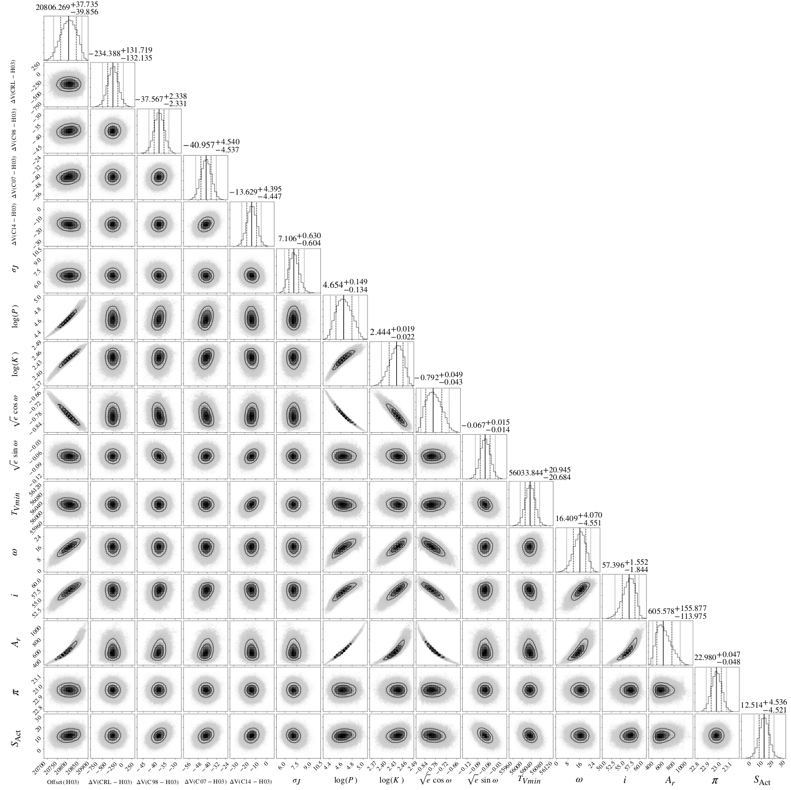
Figure 6: Marginalised 1D and 2D posterior distributions of the 16 parameters corresponding to the global fit of the RV and direct-imaging models. Confidence intervals at 2.275%, 15.85%, 50.0%, 84.15%, and 97.725% are overplotted on the 1D posterior distributions, while the median $\pm 1\leavevmode\nobreak\ \sigma$ values are given at the top of each 1D distribution. Overplotted on the 2D posterior distribution are the 1, 2, and 3 $\sigma$ contour levels. From left-to-right and top-to-bottom, the list of parameters are: $\gamma(H03)$, $\Delta V(CVL-H03)$, $\Delta V(C98-H03)$, $\Delta V(C07-H03)$, $\Delta V(C14-H03)$, $\sigma_{J}$, $\log{(P)}$, $\log{(K)}$, $\sqrt{e}.\cos{\omega}$, $\sqrt{e}.\sin{\omega}$, $T_{\rm Vmin}$, $\Omega$, $i$, $a_{r}$, $\pi$, $S_{\rm Act}$.

We note that these orbital solutions have higher eccentricities and longer periods than those published in Rickman et al. (2019). This is explained by (1) the SPHERE measurements that rule out the shortest periods and (2) a significant improvement in our MCMC implementation that increases the efficiency with which we can probe correlated parameter spaces (see Figure 6).

Table 3: Orbital elements of HD13724 B derived from the MCMC posterior distributions

Param	Unit	Med	Std	CI(2.5%)	CI(97.5%)
$P$	yr	123	41	72	226
$K$	m/s	278	13	251	299
e		0.63	0.07	0.5	0.75
$\omega$	deg	184.9	1.1	182.8	187.0
$\Omega$	deg	16.4	4.2	7.3	23.9
$i$	deg	57.4	1.7	53.6	60.9
$a_{r}$	AU	26.3	5.6	18.3	39.5
$T_{\rm Vmin}$	d	56034	21	55993	56074
$M_{\rm B}$	MJup	50.5	3.3	43.7	56.7

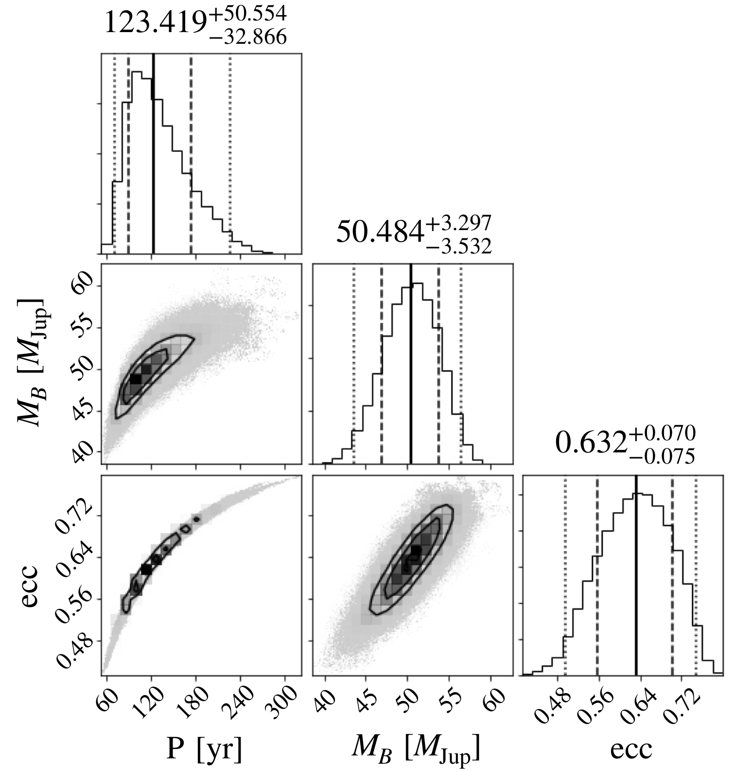
Figure 3: Marginalised 1D and 2D posterior distributions of the orbital period, as well as the eccentricity and the companion mass corresponding to the global fit of the RV and direct-imaging models. Confidence intervals at 2.275%, 15.85%, 50.0%, 84.15%, 97.725% are overplotted on the 1D posterior distributions, while the median $\pm 1\leavevmode\nobreak\ \sigma$ values are given at the top of each 1D distribution. Here, 1, 2, and 3 $\sigma$ contour levels are overplotted on the 2D posterior distribution.

4.3 Companion properties

To allow a consistent comparison with other objects and to estimate the mass of HD 13724 B, we converted the $H2$, $H3$, $J2$, $J3$, $K1$ and $K2$ fluxes into absolute magnitudes using the Gaia-measured distance of HD 13724 (Gaia Collaboration et al., 2018) shown in Table 1. We then used the COND (Baraffe et al., 2003) substellar isochrones to predict the companion mass and temperature as a function of the calculated absolute photometry in each band. The resulting absolute photometric magnitudes, masses, and temperatures are listed in Table 4.

Table 4: The measured absolute photometry of HD 13724 B with the derived mass and temperature using Baraffe et al. (2003).

Band	App. Mag	Abs. Mag	Mass	Temp.
			($M_{\mathrm{Jup}}$)	(K)
H2	17.09 $\pm$ 0.16	13.90 $\pm$ 0.16	43.9 $\pm$ 1.8	1306 $\pm$ 48
H3	17.82 $\pm$ 0.32	14.63 $\pm$ 0.32	36.7 $\pm$ 3.0	1128 $\pm$ 74
J2	18.23 $\pm$ 0.40	15.04 $\pm$ 0.40	32.4 $\pm$ 4.0	1020 $\pm$ 99
J3	17.10 $\pm$ 0.05	13.91 $\pm$ 0.05	44.0 $\pm$ 0.6	1310 $\pm$ 18
K1	16.67 $\pm$ 0.18	13.48 $\pm$ 0.18	47.5 $\pm$ 2.2	1399 $\pm$ 56
K2	17.48 $\pm$ 0.46	14.29 $\pm$ 0.46	39.0 $\pm$ 4.3	1184 $\pm$ 106

4.4 Spectral and atmospheric analysis

In order to estimate the spectral type of HD 13724 B, we used the SpeX Prism library of near-infrared (NIR) spectra of brown dwarfs (Burgasser, 2014) using the splat python package (Burgasser et al., 2016) where each spectrum was flux calibrated to the distance of HD 13724. The splat package contains a library of observed brown dwarf spectra as well as theoretical models that we use as templates to derive the physical parameters.

Each SpeX Prism spectrum was also converted into the appropriate spectral resolution of each IFS measurement by convolution with a Gaussian. The FWHM used for the convolution was assumed to be twice the separation between each wavelength channel. To fit the spectrophotometry of HD 13724 B with atmospheric models, we converted the contrast measurements into physical fluxes using a model spectrum for the host star ($T_{\mathrm{eff}}$ = 5900 K, $\log g$ = 4.5 dex and [Fe/H] = 0.3 dex) from the BT-NextGen library (Allard et al., 2012) and the SPHERE filter transmission curves. The BT-NextGen spectrum is fit to the spectral energy distribution (SED) and is built using data from Tycho (Høg et al., 2000), 2MASS (Cutri et al., 2003), WISE (Cutri & et al., 2013), and HIPPARCOS (Perryman et al., 1997).

We calculated the $\chi_{r}^{2}$ of template brown dwarfs in the SpeX Prism library as a function of spectral type. We include the uncertainties of the template spectra in the $\chi^{2}$ computation. The best-fit object is 2MASS J10595185+3042059 (Cutri et al., 2003) which is classified as a T4 brown dwarf. In Fig. 5 we also plot the second-best fit spectrum of SDSSp J092615.38+584720.9 (Cutri et al., 2003), which is classified as a T4.0/T4.5 brown dwarf. The temperatures of 2MASS J10595185+3042059 and SDSSp J092615.38+584720.9 are not given explicitly but effective temperatures of mid-T dwarfs covers a small range ($T_{\mathrm{eff}}\approx 1100-1400$ K Kirkpatrick et al. (2000)). The T4 spectral type provides the best fit.

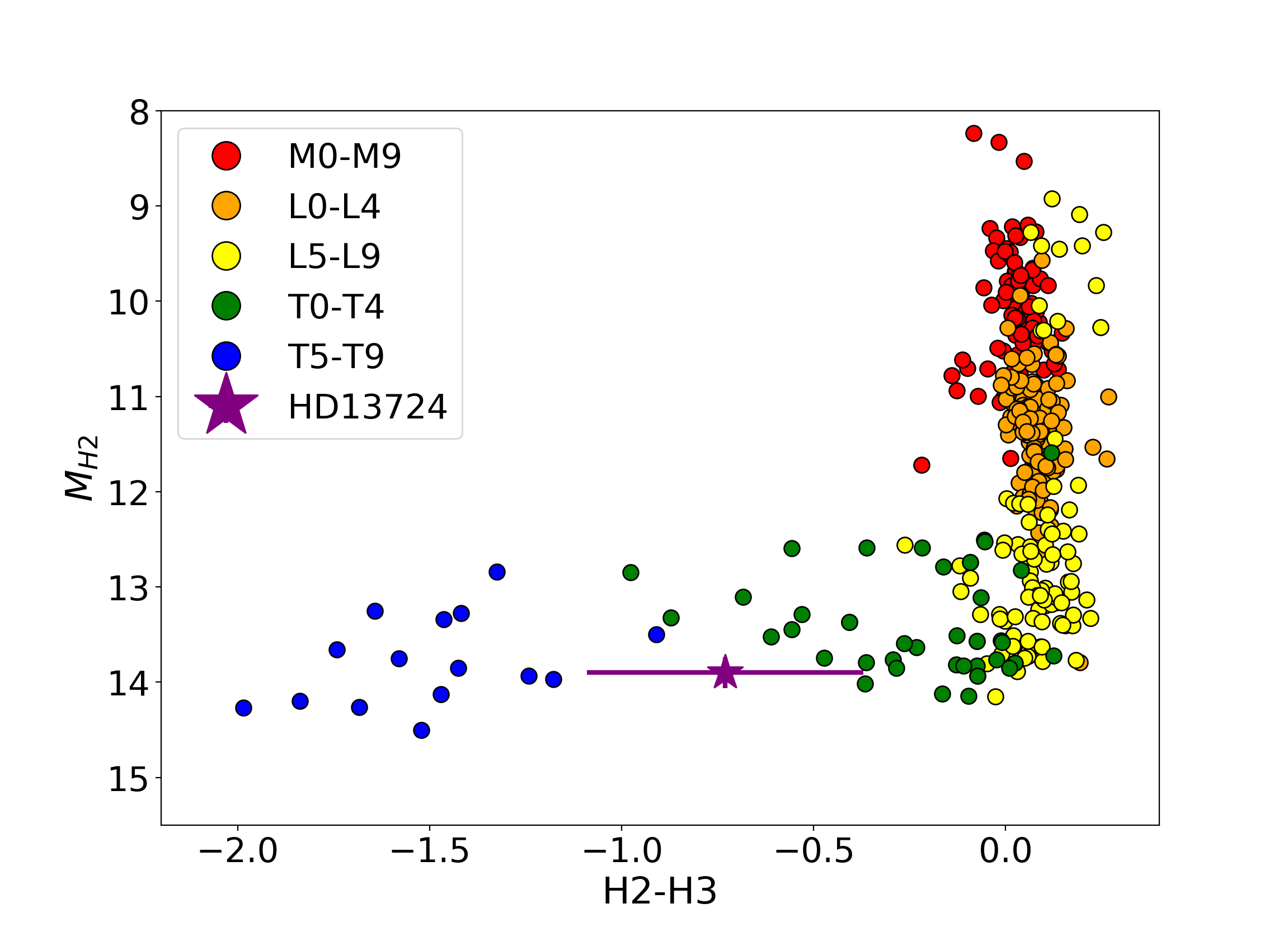
Figure 4: Colour-magnitude diagram showing the predicted H2-H3 colours and H2 absolute magnitudes for objects in the SpeX Prism Library (Burgasser, 2014). The flux of HD 13724 B and the 1$\sigma$ limit on its H2-H3 colour are shown. Its position is compatible with objects in the middle of the T sequence.

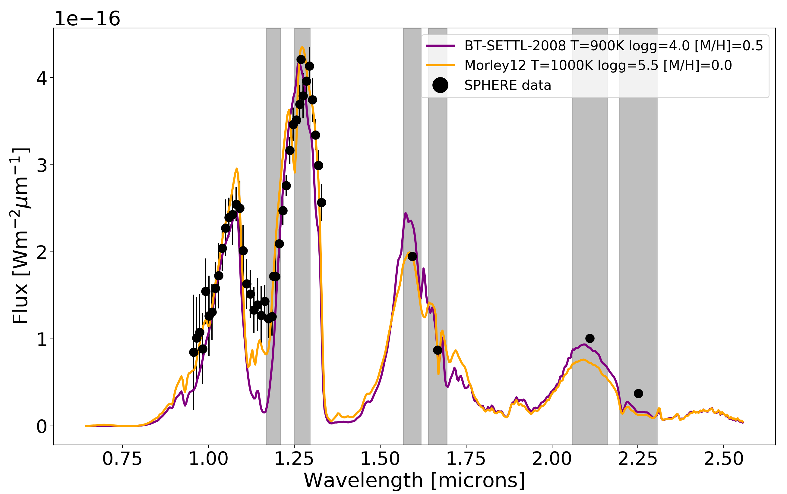
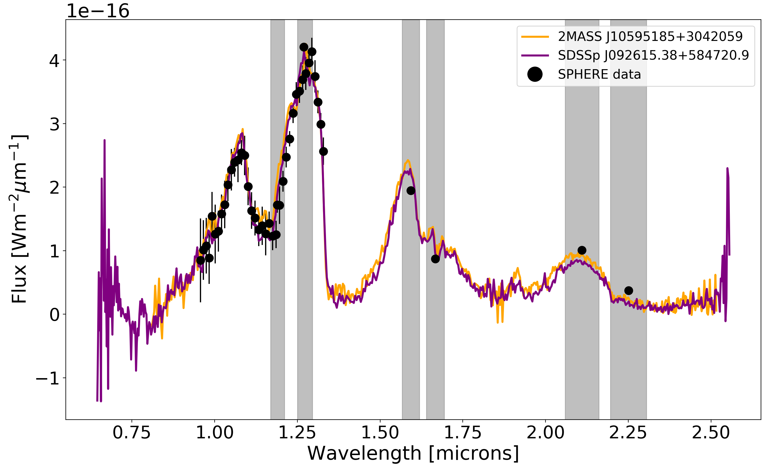
Figure 5: Atmospheric spectra of HD 13724. The FWHM of the $J23$, $H23,$ and $K12$ IRDIS filters are shown with grey bars (from left to right). The error bars on the $H2$, $H3$, $K1,$ and $K2$ data are present but smaller than the size of the markers on each plot. Top: The two best-fitting spectra from BT-Settl 2008 models (Allard et al., 2012) and the Morley et al. (2012) models from the SpeX Prism library are overplotted, and the flux is scaled to match HD 13724 B. Fitting was performed to the IFS and IRDIS data simultaneously. Bottom: Comparison of the observed spectrum of HD 13724 B with the two best fit T4 brown dwarf atmospheres: 2MASS J10595185+3042059 and SDSSp J092615.38+58720.9 fitted using the splat package (Burgasser et al., 2016).

We use the $H2$ and $H3$ band values to place HD 13724 B on a colour-magnitude diagram as shown in Fig. 4 which is built using the Spex Prism Library (Burgasser, 2014). The placement of HD 13724 B on the colour-magnitude diagram agrees well with the estimated T spectral type.

To further constrain the physical properties of HD 13724 B, we compared the observed SED to synthetic spectra for cool brown dwarfs from Morley et al. (2012) and Allard et al. (2012). The biggest difference between these models is that the Morley et al. (2012) models include the condensate sedimentation efficiency coefficients.

We adjusted the Morley et al. (2012) and Allard et al. (2012) models, which sit well within the range of the mid-T dwarf range (see Fig. 5). The Morley et al. (2012) models are the best fit to the data with the following parameters: $T_{\mathrm{eff}}$ = 1000 K, $\log g=5.5\mathrm{cm}/\mathrm{s}^{2}$, $f_{\mathrm{SED}}$ = 3, [M/H] = 0.0, and $R=1.01\leavevmode\nobreak\ R_{\mathrm{Jup}}$.

5 Summary and conclusions

In this paper we report the direct detection of a $\sim$ 50 $M_{\mathrm{Jup}}$ brown dwarf using VLT/SPHERE. HD 13724 B serves as an essential benchmark brown dwarf for testing brown dwarf atmospheric and evolutionary models where it joins just a short list of benchmark brown dwarf companions of stars with RV and imaging measurements: HR 7672 B (Liu et al., 2002; Crepp et al., 2012), HD 19467 B (Crepp et al., 2014), HD 4747 B (Sahlmann et al., 2011; Crepp et al., 2016; Peretti et al., 2019), GJ 758 B (Thalmann et al., 2009; Bowler et al., 2018), HD 4113 C (Cheetham et al., 2018), GJ 229 B (Nakajima et al., 1995; Brandt et al., 2019; Feng et al., 2020), and HD 72946 B (Maire et al., 2019).

We obtained images of HD 13724 B in the J, H, and K bands along with its spectrum from IFS data in the $Y-J$ bands. Through comparison with the SpeX Prism Library of brown dwarf spectra (Burgasser, 2014), we found that HD 13724 B is most consistent with a spectral type of T4, which also agrees with the position of HD 13724 B on the $H2-H3$ colour-magnitude diagram (Fig. 4). It should be noted that in general the template T4 brown dwarf provides a better fit than the synthetic spectra of Morley et al. (2012). This is especially true in the $K1$ and $K2$ bands where we observe more flux than the models would suggest. This might be due to clouds in the atmospheres that tend to increase the flux in the $K$-band (Marley et al., 1996; Morley et al., 2012). The template adjustment using the Morley et al. (2012) models allowed us to derive a temperature of $1000\leavevmode\nobreak\ K$.

We analysed the HD 13724 system by combining RV measurements and high-contrast imaging, enabling us to place constraints on the orbital and physical parameters of HD 13724 B. This suggests a mass of 43-56 $M_{\mathrm{Jup}}$, an inclination of 53-60 deg, and a period range of 72-226 years. We calculated the isochronal mass of HD 13724 B from the COND substellar isochrones (Baraffe et al., 2003) taking into account the age of the star. This gives a mass range of 31-52 $M_{\mathrm{Jup}}$ corresponding to an age of 0.5-2 Gyr. This overlaps with the mass range from the observations and suggests that either the star is slightly older than expected or – if the age is correct – some physics is missing from the modelling of the evolution of these substellar objects.

The combination of Gaia astrometry with future RV and imaging datasets will allow for much tighter constraints on the orbital and physical parameters of HD 13724 B, which in turn will improve the comparison with atmospheric and evolutionary models.

Many attempts have been made to detect these long-period companions from the CORALIE RV survey through imaging as part of a fifteen-year effort using VLT/NACO, with little success. The VLT/SPHERE is allowing us to now unveil these RV-detected brown dwarfs. We expect that the future upgrade of SPHERE (SPHERE+ Boccaletti, 2019) will increase the sample of cool brown dwarfs detected thanks to its higher contrast capabilities at short separations. Ultimately, future instruments like SPHERE+, the James Webb Space Telescope, and the upcoming ELT/METIS (Carlomagno et al., 2016) should allow us to bridge the gap between the coolest brown dwarfs and the most massive giant planets.

Appendix A MCMC results

Here we provide the full list of parameters adjusted in the MCMC as well as the marginalised 1D and 2D posterior distributions of the parameters corresponding to the global fit of the RV and direct-imaging models.

Table 5: Parameters corresponding to the combined adjustment of the astrometric and RV observations of HD13724 AB derived from the MCMC posterior distributions.

Var	Units	Max(Proba)	Mode	Med	Std	CI(2.5%)	CI(97.5%)	Priors
M⋆	[M⊙]							$N(1.14,0.06)$
$\pi$	[mas]							$N(22.9781,\sqrt{0.0277^{2}+0.040^{2}})$
$\log{(\rm Proba)}$		-675.516	-685.396	-682.013	2.687	-688.373	-678.024
$\gamma(H03$)	[m/s]	20833	20885	20806	36	20733	20870	$U$
$\Delta V(CVL-H03)^{*}$	[m/s]	-229	-303	-234	133	-496	27	$N(0,300)$
$\Delta V(C98-H03)$	[m/s]	-37.9	-35.8	-37.6	2.3	-42.2	-33.0	$U$
$\Delta V(C07-H03)$	[m/s]	-37.8	-34.2	-41.0	4.5	-49.9	-32.2	$U$
$\Delta V(C14-H03)$	[m/s]	-15.1	-21.2	-13.6	4.4	-22.3	-5.0	$N(-20,5)$
$S_{\rm Act}$	[m/s]	14.0	20.3	12.5	4.5	3.6	21.4	$U$
$\sigma_{J}$	[m/s]	7.03	7.17	7.11	0.62	5.98	8.39	$U$
$\log{(P)}$	[day]	4.764	4.952	4.654	0.132	4.423	4.917	$U$
$\log{(K)}$	[m/s]	2.459	2.483	2.444	0.020	2.400	2.476	$U$
$\sqrt{e}.\cos{\omega}$		-0.827	-0.864	-0.792	0.043	-0.862	-0.702	$U$
$\sqrt{e}.\sin{\omega}$		-0.070	-0.114	-0.067	0.014	-0.095	-0.039	$U$
$T_{\rm Vmin}$	[bjd]∗∗	56033	56038	56034	21	55993	56074	$U$
$\Omega$	[deg]	17.4	19.2	16.4	4.3	7.3	23.9	$U$
$i$	[deg]	58.5	58.6	57.40	1.7	53.6	60.0	$U$
$a_{r}$	[mas]	721	945	606	129	421	907	$U$
K	[m/s]	288	304	278	13	251	299	-
P	[y]	159	245	123	41	72	226	-
$e$		0.688	0.760	0.632	0.067	0.498	0.747	-
$\omega$	[deg]	184.9	187.5	184.9	1.1	182.8	187.0	-
$a_{r}$	[au]	31.3	41.2	26.3	5.6	18.3	39.5	-
MB	[Mjup]	53.1	56.3	50.5	3.3	43.7	56.4	-
M${}_{B}.\sin(i)$	[Mjup]	45.3	48.1	42.5	3.5	35.3	48.6	-
*: CVL stands for CORAVEL; **: The date is expressed as BJD-2400000.