Partial Optimal Transport
with Applications on Positive-Unlabeled Learning

Abstract

Classical optimal transport problem seeks a transportation map that preserves the total mass betwenn two probability distributions, requiring their mass to be the same. This may be too restrictive in certain applications such as color or shape matching, since the distributions may have arbitrary masses and/or that only a fraction of the total mass has to be transported. Several algorithms have been devised for computing partial Wasserstein metrics that rely on an entropic regularization, but when it comes with exact solutions, almost no partial formulation of neither Wasserstein nor Gromov-Wasserstein are available yet. This precludes from working with distributions that do not lie in the same metric space or when invariance to rotation or translation is needed. In this paper, we address the partial Wasserstein and Gromov-Wasserstein problems and propose exact algorithms to solve them. We showcase the new formulation in a positive-unlabeled (PU) learning application. To the best of our knowledge, this is the first application of optimal transport in this context and we first highlight that partial Wasserstein-based metrics prove effective in usual PU learning settings. We then demonstrate that partial Gromov-Wasserstein metrics is efficient in scenario where point clouds come from different domains or have different features.

1 Introduction

Optimal transport (OT) has been gaining in recent years an increasing attention in the machine learning community. This success is due to its capacity to exploit the geometric property of the samples at hand. Generally speaking, OT is a mathematical tool to compare distributions by computing a transportation mass plan from a source to a target distribution. Distances based on OT are referred to as the Monge-Kantorovich or Wasserstein distances (Villani, 2009) and have been successfully employed in a wide variety of machine learning applications including clustering (Ho et al., 2017), computer vision (Bonneel et al., 2011; Solomon et al., 2015), generative adversarial networks (Arjovsky et al., 2017) or domain adaptation (Courty et al., 2017).

A key limitation of Wasserstein distance is that it relies on the assumption of aligned distributions, namely they must belong to the same ground space or that at least a meaningful distance across domains can be computed. Nevertheless, source and target distributions can be collected under distinct environments, representing different times of collection, contexts or measurements (see Fig. 1, left and right). To get benefit from OT on such heterogeneous distribution settings, one can compute the Gromov-Wasserstein (GW) distance (Sturm, 2006; Mémoli, 2011) to overcome the lack of intrinsic correspondence between the distribution spaces. GW extends Wasserstein by computing a distance between metrics defined within each of the source and target spaces. From a computational point view, it involves a non convex quadratic problem, hard to lift to large scale settings (Peyré and Cuturi, 2019). A remedy to a such heavy computation burden lies in a prevalent approach referred to as regularized OT (Cuturi, 2013), allowing one to add an entropic regularization penalty to the original problem.  Peyré et al. (2016) proposed the entropic GW discrepancy, that can be solved by Sinkhorn iterations (Cuturi, 2013; Benamou et al., 2015).

A major bottleneck of OT in its traditional formulation is that it requires the two input measures to have the same total probability mass and/or that all the mass has to be transported. This is too restrictive for many applications since mass changes may occur due to a creation or an annihilation while computing an OT plan. To tackle this limitation, one may employ strategies such as partial or unbalanced transport (Guittet, 2002; Figalli, 2010; Caffarelli and McCann, 2010).  Chizat et al. (2018) propose to relax the marginal constraints of unbalanced total masses using divergences such as Kullback-Leibler or Total Variation, allowing the use of generalized Sinkhorn iterations.  Yang and Uhler (2019) generalize this approach to GANs and  Lee et al. (2019) present an ADMM algorithm for the relaxed partial OT. Most of all these approaches concentrate on partial-Wasserstein.

This paper deals with exact partial Wassertein (partial-W) and Gromov-Wasserstein (partial-GW). Standard strategies for computing such partial-W require relaxations of the marginals constraints. We rather build our approach upon adding virtual or dummy points onto the marginals, in the same spirit as Caffarelli and McCann (2010). These points are used as a buffer when comparing distributions with different probability masses, allowing partial-W to boil down to solving an extended but standard Wasserstein problem. The main advantage of this approach is that it leads to computing sparse transport plans and hence exact partial-W or GW distances instead of regularized discrepancies obtained by running Sinkhorn algorithms. Regarding partial-GW, our approach relies on a Frank-Wolfe optimization algorithm (Frank and Wolfe, 1956) that builds on computations of partial-W.

Tackling partial-OT problems that preserve sparsity is motivated by the fact that they are more suitable to some applications such as the Positive-Unlabeled (PU) learning, see Bekker and Davis (2020) for a review, we target in this paper. We shall notice that this is the first application of OT for solving PU learning tasks. In a nutshell, PU classification is a variant of binary classification problem, in which we have only access to labeled samples from positive (Pos) class in the training stage. The aim is to assign classes to the points of an unlabeled (Unl) set which mixes data from both positive and negative classes. Using OT allows identifying the positive points within Unl, even when Pos and Unl samples do not lie in the same space (see Fig. 1).

The paper is organized as follows: we first recall some background on OT. In Section 3, we propose an algorithm to solve an exact partial-W problem, together with a Frank-Wolfe based algorithm to compute the partial-GW solution. After describing in more details the PU learning task and the use of partial-OT to solve it, we illustrate the advantage of partial-GW when the source and the target distributions are collected onto distinct environments. We finally give some perspectives.

Notations

$\Sigma_{N}$ is an histogram of $N$ bins with $\left\{\bm{p}\in\mathbb{R}_{+}^{N},\sum_{i}p_{i}=1\right\}$ and $\delta$ is the Dirac function. Let $\mathbbm{1}_{n}$ be the $n$-dimensional vector of ones. $\langle\cdot,\cdot\rangle_{F}$ stands for the Frobenius dot product. $|\bm{p}|$ indicates the length of vector $\bm{p}$.

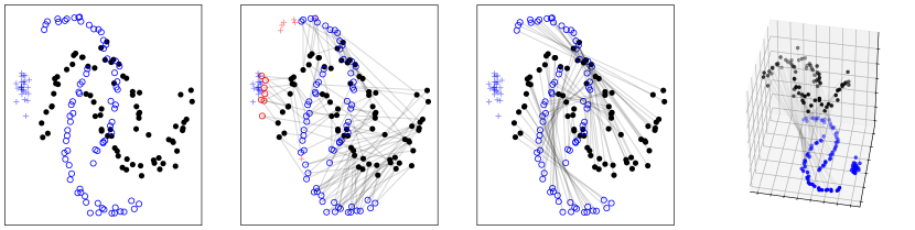
Figure 1: (Left) Source (in black) and target (in blue) distributions that have been collected under distinct environments. The source domain contains only positive points ($o$) whereas the target domain contains both positives and negatives ($+$) (Middle left) Partial-W fails to assign correctly all the labels in such context, red symbols indicating wrong assignments (Middle right) Partial-GW recovers the correct labels of the unlabeled samples, with a consistent transportation plan (gray lines), even when the dataset do not live in the same state space (Right).

2 Background on optimal transport

Let $\mathcal{X}=\{\bm{x}_{i}\}_{i=1}^{n}$ and $\mathcal{Y}=\{\bm{y}_{j}\}_{j=1}^{m}$ be two point clouds representing the source and target samples, respectively. We assume two empirical distributions $(\bm{p},\bm{q})\in\Sigma_{n}\times\Sigma_{m}$ over $\mathcal{X}$ and $\mathcal{Y}$,

$$\bm{p}=\sum_{i=1}^{n}p_{i}\delta_{\bm{x}_{i}}\quad\text{ and }\quad\bm{q}=\sum_{j=1}^{m}q_{j}\delta_{\bm{y}_{j}},$$

where $\Sigma_{n}$ and $\Sigma_{m}$ are histograms of $|\bm{p}|=n$ and $|\bm{q}|=m$ bins respectively. The set of all admissible couplings $\Pi(\bm{p},\bm{q})$ between histograms is given by

$$\Pi(\bm{p},\bm{q})=\{\bm{T}\in{\mathbb{R}}_{+}^{|\bm{p}|\times|\bm{q}|}|\bm{T}\mathbbm{1}_{|\bm{q}|}=\bm{p},\bm{T}^{\top}\mathbbm{1}_{|\bm{p}|}=\bm{q}\},$$

where $\bm{T}=\left(T_{ij}\right)_{i,j}$ is a coupling matrix with an entry $T_{ij}$ that describes the amount of mass $p_{i}$ found at $\bm{x}_{i}$ flowing toward the mass $q_{j}$ of $\bm{y}_{j}$.

OT addresses the problem of optimally transporting $\bm{p}$ toward $\bm{q}$, given a cost $D_{ij}$ measured as a geometric distance between $\bm{x}_{i}$ and $\bm{y}_{j}$. More precisely, when the ground cost $\bm{C}=\mathbf{D}^{p}=\left(D_{ij}^{p}\right)_{i,j}$ is a distance matrix, the $p$-Wassertein distance on $\Sigma_{n}\times\Sigma_{m}$ at the power of $p$ is defined as:

$$W_{p}^{p}(\bm{p},\bm{q})=\min_{\bm{T}\in\Pi(\bm{p},\bm{q})}\langle\bm{C},\bm{T}\rangle_{F}=\min_{\bm{T}\in\Pi(\bm{p},\bm{q})}\sum_{i=1}^{n}\sum_{j=1}^{m}C_{ij}T_{ij}.$$

In some applications, the two distributions are not registered (i.e. we can not compute a ground cost between $\bm{x}_{i}$ and $\bm{y}_{j}$) or do not lie in the same underlying space. The Gromov-Wasserstein distance addresses this bottleneck by extending the Wasserstein distance to such settings, also allowing invariance to translation, rotation or scaling. It relies on intra-domain distance matrices of source $\bm{C}^{s}=(C^{s}_{ik})_{i,k}=(C^{s}(\bm{x}_{i},\bm{x}_{k}))_{i,k}\in\mathbb{R}_{+}^{n\times n}$ and target $\bm{C}^{t}=(C^{t}_{jl})_{j,l}=(C^{t}(\bm{y}_{j},\bm{y}_{l}))_{j,l}\in\mathbb{R}_{+}^{m\times m}$, and is defined as in Mémoli (2011):

$$GW_{p}^{p}(\bm{p},\bm{q})=\min_{\bm{T}\in\Pi(\bm{p},\bm{q})}\sum_{i,k=1}^{n}\sum_{j,l=1}^{m}\left|C^{s}_{ik}-C^{t}_{jl}\right|^{p}T_{ij}T_{kl}.$$

3 Exact Partial Wasserstein and Gromov-Wasserstein distance

3.1 Partial Wasserstein distance

The previous OT distances require the two distributions to have the same total probability mass $\|\bm{p}\|_{1}=\|\bm{q}\|_{1}$ and that all the mass has to be transported. This may be a problematic assumption where some mass variation or partial mass displacement should be handled. The partial OT problem focuses on transporting only a fraction $0\leq s\leq\min(\|\bm{p}\|_{1},\|\bm{q}\|_{1})$ of the mass as cheaply as possible. In that case, the set of admissible couplings becomes

$$\Pi^{u}(\bm{p},\bm{q})=\{\bm{T}\in{\mathbb{R}}_{+}^{|\bm{p}|\times|\bm{q}|}|\bm{T}\mathbbm{1}_{|\bm{q}|}\leq\bm{p},\bm{T}^{\top}\mathbbm{1}_{|\bm{p}|}\leq\bm{q},\mathbbm{1}_{|\bm{p}|}^{\top}\bm{T}\mathbbm{1}_{|\bm{q}|}=s\},$$

and the partial-W distance reads as $PW^{p}_{p}(\bm{p},\bm{q})=\min_{\bm{T}\in\Pi^{u}(\bm{p},\bm{q})}\sum_{i=1}^{n}\sum_{j=1}^{m}\langle\bm{C},\bm{T}\rangle_{F}.$ This problem has been studied by Caffarelli and McCann (2010); Figalli (2010); numerical solutions has notably been provided by Benamou et al. (2015); Chizat et al. (2018) in the entropic-regularized Wasserstein case. We propose here to solve the exact partial-W problem by adding dummy or virtual points $\bm{x}_{n+1}$ and $\bm{y}_{m+1}$ (with any features) and extending the cost matrix as follows:

$$\bar{\bm{C}}=\begin{bmatrix}\bm{C}&\xi\mathbbm{1}_{|\bm{q}|}\\ \xi\mathbbm{1}_{|\bm{p}|}^{\top}&2\xi+A\end{bmatrix}$$ (1)

in which $A>\max(C_{ij})$ and $\xi$ is a bounded scalar. When the mass of these dummy points is set such that $p_{n+1}=\|\bm{q}\|_{1}-s$ and $q_{m+1}=\|\bm{p}\|_{1}-s$, computing partial-W distance boils down to solving a unconstrained problem $W_{p}^{p}(\bar{\bm{p}},\bar{\bm{q}})=\min_{{\bar{\bm{T}}}\in\Pi(\bar{\bm{p}},\bar{\bm{q}})}\langle\bar{\bm{C}},\bar{\bm{T}}\rangle_{F}$, where $\bar{\bm{p}}=[\bm{p},\|\bm{q}\|_{1}-s]$ and $\bar{\bm{q}}=[\bm{q},\|\bm{p}\|_{1}-s]$. The intuitive derivation of this equivalent formulation is exposed in Appendix A.1.

Proposition 1

Assume that $A>\max(C_{ij})$ and that $\xi$ is bounded, one has

$$W_{p}^{p}(\bar{\bm{p}},\bar{\bm{q}})-PW^{p}_{p}(\bm{p},\bm{q})=\xi(\|\bm{p}\|_{1}+\|\bm{q}\|_{1}-2s)$$

and the optimum transport plan $\bm{T}^{*}$ of the partial Wasserstein problem is the optimum transport plan $\bar{\bm{T}}^{*}$ of $W_{p}^{p}(\bar{\bm{p}},\bar{\bm{q}})$ deprived from its last row and column.

The proof is postponed to Appendix A.2.

3.2 Partial Gromov-Wasserstein

We are now interested in the partial extension of Gromov-Wasserstein. In the case of a quadratic cost, $p=2$, and the partial-GW problem writes as

$$PGW_{2}^{2}(\bm{p},\bm{q})=\min_{\bm{T}\in\Pi^{u}(\bm{p},\bm{q})}\mathcal{J}_{\bm{C}^{s},\bm{C}^{t}}(\bm{T})$$

where

$$\mathcal{J}_{\bm{C}^{s},\bm{C}^{t}}(\bm{T})=\frac{1}{2}\sum_{i,k=1}^{n}\sum_{j,l=1}^{m}(C^{s}_{ik}-C^{t}_{jl})^{2}T_{ij}T_{kl}.$$ (2)

This loss function $\mathcal{J}_{\bm{C}^{s},\bm{C}^{t}}$ is non-convex and the couplings feasibility domain $\Pi^{u}(\bm{p},\bm{q})$ is convex and compact. One may expect to introduce virtual points in the GW formulation in order to solve the partial-GW problem. Nevertheless, this strategy is no longer valid as it involves pairwise distances that do not allow the computations related to the dummy points to be isolated (see Appendix A.3).

In the following, we build upon a Frank-Wolfe optimization scheme (Frank and Wolfe, 1956) a.k.a. the conditional gradient method (Demyanov and Rubinov, 1970). It has received significant renewed interest in machine learning (Jaggi, 2013; Lacoste-Julien and Jaggi, 2015) and in OT community, since it serves as a basis to approximate penalized OT problems (Ferradans et al., 2013; Courty et al., 2017) or GW distances (Peyré et al., 2016; Vayer et al., 2018). Our proposed Frank-Wolfe iterations strongly rely on computing partial-W distances and as such, achieve a sparse transport plan (Ferradans et al., 2013).

Let us first introduce some additional notations. For any tensor $\mathcal{M}=(\mathcal{M}_{ijkl})_{i,j,k,l}\in{\mathbb{R}}^{n\times n\times m\times m}$, we denote by $\mathcal{M}\circ\bm{T}$ the matrix in ${\mathbb{R}}^{n\times m}$ such that its $(i,j)$-th element is defined as

$$(\mathcal{M}\circ\bm{T})_{i,j}=\sum_{k=1}^{n}\sum_{l=1}^{m}\mathcal{M}_{ijkl}T_{kl}$$

for all $i=1,\ldots,n,j=1,\ldots,m.$ Introducing the $4$-th order tensor $\mathcal{M}(\bm{C}^{s},\bm{C}^{t})=\frac{1}{2}((C^{s}_{ik}-C^{t}_{jl})^{2})_{i,j,k,l},$ we notice that $\mathcal{J}_{\bm{C}^{s},\bm{C}^{t}}(\bm{T})$, following Peyré et al. (2016), can be written as

$$\mathcal{J}_{\bm{C}^{s},\bm{C}^{t}}(\bm{T}) =\langle\mathcal{M}(\bm{C}^{s},\bm{C}^{t})\circ\bm{T},\bm{T}\rangle_{F}.$$

The Frank-Wolfe algorithm for partial-GW is shown in Algorithm 1. Like classical Frank-Wolfe procedure, it is summarized in three steps for each iteration $k$, as detailed below. A theoretical study of the convergence of the Frank-Wolfe based algorithm for partial-GW is given in Appendix B.2. Also detailed derivation of the line search step is provided in the supplementary material.

Step1

Compute a linear minimization oracle over the set $\Pi^{u}(\bm{p},\bm{q})$, i.e.,

$$\widetilde{\bm{T}}^{(k)}\leftarrow\operatorname*{\arg\!\min}_{\bm{T}\in\Pi^{u}(\bm{p},\bm{q})}\langle\nabla\mathcal{J}_{\bm{C}^{s},\bm{C}^{t}}(\bm{T}^{(k)}),\bm{T}\rangle_{F},$$ (3)

To do so, we solve an extended Wasserstein problem with the ground metric $\nabla\mathcal{J}_{\bm{C}^{s},\bm{C}^{t}}(\bm{T}^{(k)})$ extended as in eq. (1):

$$\bar{\bm{T}}^{(k)}\leftarrow\operatorname*{\arg\!\min}_{\bm{T}\in\Pi(\bar{\bm{p}},\bar{\bm{q}})}\langle\bar{\nabla}\mathcal{J}_{\bm{C}^{s},\bm{C}^{t}}(\bm{T}^{(k)}),\bm{T}\rangle_{F},$$ (4)

and get $\widetilde{\bm{T}}^{(k)}$ from $\bar{\bm{T}}^{(k)}$ by removing its last row and column.

Step2

Determine optimal step-size $\gamma^{(k)}$ subject to

$$\gamma^{(k)}\leftarrow\operatorname*{\arg\!\min}_{\gamma\in[0,1]}\{\mathcal{J}_{\bm{C}^{s},\bm{C}^{t}}((1-\gamma)\bm{T}^{(k)}+\gamma\widetilde{\bm{T}}^{(k)})\}.$$ (5)

It can be shown that $\gamma^{(k)}$ can take the following values, with $\bm{E}^{(k)}=\widetilde{\bm{T}}^{(k)}-{\bm{T}}^{(k)}$:

• if $\langle\mathcal{M}(\bm{C}^{s},\bm{C}^{t})\circ\bm{E}^{(k)},\bm{E}^{(k)}\rangle_{F}<0$ we have

  $$\gamma^{(k)}=\left\{\begin{array}[]{ll}0&\mbox{if }\langle\mathcal{M}(\bm{C}^{s},\bm{C}^{t})\circ\bm{E}^{(k)},\bm{E}^{(k)}\rangle_{F}+2\langle\mathcal{M}(\bm{C}^{s},\bm{C}^{t})\circ\bm{E}^{(k)},\bm{T}^{(k)}\rangle_{F}>0\\ 1&\mbox{otherwise.}\end{array}\right.$$

• if $\langle\mathcal{M}(\bm{C}^{s},\bm{C}^{t})\circ\bm{E}^{(k)},\bm{E}^{(k)}\rangle_{F}>0$ we have

  $$\gamma^{(k)}=\min\left(1,\max\left(0,-\frac{\langle\mathcal{M}(\bm{C}^{s},\bm{C}^{t})\circ\bm{E}^{(k)},\bm{T}^{(k)}\rangle_{F}}{\langle\mathcal{M}(\bm{C}^{s},\bm{C}^{t})\circ\bm{E}^{(k)},\bm{E}^{(k)}\rangle_{F}}\right)\right)$$

Step3

Update ${\bm{T}}^{(k+1)}\leftarrow(1-\gamma^{(k)}){\bm{T}}^{(k)}+\gamma^{(k)}\widetilde{\bm{T}}^{(k)}$.

Algorithm 1 Frank-Wolfe algorithm for partial-GW

1:  Input: Source and target samples: $(\mathcal{X},\bm{p})$ and $(\mathcal{Y},\bm{q})$, mass $s$, $p=2$, initial guess $\bm{T}^{(0)}$

2:  Compute cost matrices $\bm{C}^{s}$ and $\bm{C}^{t}$, build $\bar{\bm{p}}$ and $\bar{\bm{q}}$

3:  for $k=1,2,3,\ldots$ do

4:     $\bm{G}^{(k)}\leftarrow\mathcal{M}(\bm{C}^{s},\bm{C}^{t})\circ\bm{T}^{(k-1)}$ // Gradient computation

5:     $\bar{\bm{T}}^{(k)}\leftarrow\operatorname*{\arg\!\min}_{\bm{T}\in\Pi(\bar{\bm{p}},\bar{\bm{q}})}\langle\bar{\bm{G}}^{(k)},\bm{T}\rangle_{F}$ // Compute partial-W

6:     Get $\widetilde{\bm{T}}^{(k)}$ from $\bar{\bm{T}}^{(k)}$ // Remove last row and column

7:     Compute $\gamma^{(k)}$ as in Eq. (5) // Line-search

8:     ${\bm{T}}^{(k+1)}\leftarrow(1-\gamma^{(k)}){\bm{T}}^{(k)}+\gamma^{(k)}\widetilde{\bm{T}}^{(k)}$ // Update

9:  end for

10:  Return: ${\bm{T}}^{(k)}$

4 Optimal transport for PU learning

We hereafter investigate the application of partial optimal transport for learning from Positive and Unlabeled (PU) data. After introducing the PU learning, we present how to adapt the formulation of partial-OT to this setting.

4.1 Overview of PU learning

Learning from PU data is a variant of classical binary classification problem, in which the training data consist of only positive points, and the test data is composed of unlabeled positives and negatives. Let ${\bf{Pos}}=\{\bm{x}_{i}\}_{i=1}^{n_{P}}$ be the positive samples drawn according to the conditional distribution $p(\bm{x}|y=1)$ and ${\bf{Unl}}=\{\bm{x}_{i}^{U}\}_{i=1}^{n_{U}}$ the unlabeled set sampled according to the marginal $p(\bm{x})=\pi p(\bm{x}|y=1)+(1-\pi)p(\bm{x}|y=-1)$. The true proportion of positives, called class prior, is $\pi=p(y=1)$ and $p(\bm{x}|y=-1)$ is the distribution of negative samples which are all unlabeled.The goal is to learn a binary classifier solely using Pos and Unl. A broad overview of existing PU learning approaches can be seen in (Bekker and Davis, 2020).

Most PU learning methods commonly rely on the selected completely at random (SCAR) assumption (Elkan and Noto, 2008), which assumes that the labeled samples are drawn at random among the positive distribution, independently of their attributes. Nevertheless, this assumption is often violated in real-case scenarios and PU data are often subject to selection biases, e.g. when part of the data may be easier to collect. Recently, a less restrictive assumption has been studied: the selected at random (SAR) setting (Bekker and Davis, 2018) which assumes that the positives are labeled according to a subset of features of the samples. Kato et al. (2019) move a step further and consider that the sampling scheme of the positives is such that $p(o=1|\bm{x},y=1)$ ($o=1$ means observed label) preserves the ordering over the samples induced by the posterior distribution $p(y=1|\bm{x},y=1)$. Other approaches, as in (Hsieh et al., 2019), consider a classical PU learning problem adjuncted with a small proportion of observed negative samples. Those negatives are selected with bias following the distribution $p(\bm{x}|y=-1)$.

4.2 PU learning formulation using partial optimal transport

We propose in this paper to use partial optimal transport to perform PU learning. In that context, the unlabeled points Unl represent the source distribution $\mathcal{X}$ and the positive points Pos are the target dataset $\mathcal{Y}$. We set the total probability mass to be transported $s=\pi$ as the proportion of positives in the unlabeled set. As such, the transport matrix $\bm{T}$ should be such that the unlabeled positive points are mapped to the positive samples (as they have similar features or intra-domain distance matrices) while the negatives are discarded (in our context, they are not tranported at all). We look for an optimal transport plan that belongs to the following set of couplings, assuming $n=n_{U}$, $m=n_{P}$, $p_{i}=\frac{1}{n}$ and $q_{j}=\frac{1}{m}$:

$$\Pi^{PU}(\bm{p},\bm{q})=\{\bm{T}\in{\mathbb{R}}_{+}^{|\bm{p}|\times|\bm{q}|}|\bm{T}\mathbbm{1}_{|\bm{q}|}=\{\bm{p},0\},\bm{T}^{\top}\mathbbm{1}_{|\bm{p}|}\leq\bm{q},\mathbbm{1}_{|\bm{p}|}^{\top}\bm{T}\mathbbm{1}_{|\bm{q}|}=s\},$$ (6)

in which $\bm{T}\mathbbm{1}_{|\bm{q}|}=\{\bm{p},0\}$ means that $\sum_{j=1}^{m}T_{ij}=p_{i}$ exactly or 0, $\forall i$ to avoid matching a unlabeled negative with a positive. This set is not empty as long as $s\mod p_{i}=0$. Though the positive samples Pos are assumed easy to label, their features may be corrupted with noise or they may be mislabeled. Let assume $0\leq\alpha\leq 1-s$, the noise level.

To solve the Wasserstein problem with the admissible constraint set (6) related to this PU learning, we adopt a regularized point of view of the partial-OT problem as in Courty et al. (2017):

$$\bar{\bm{T}}^{*}=\operatorname*{\arg\!\min}_{\bar{\bm{T}}\in\Pi(\bar{\bm{p}},\bar{\bm{q}})}\sum_{i=1}^{n+1}\sum_{j=1}^{m+1}\bar{C}_{ij}\bar{T}_{ij}+\eta\Omega(\bar{\bm{T}})$$ (7)

where $p_{i}=\frac{1-\alpha}{n}$, $q_{j}=\frac{s+\alpha}{m}$, and $\bar{\bm{q}}$, $\bar{C}_{ij}$ are defined as in Section 3.1, $\eta\geq 0$ is a regularization parameter and $\alpha$ is the percentage of Pos that we assume to be noisy (that is to say we do not want to match them with Unl). We choose $\Omega(\bar{\bm{T}})=\sum_{i}\sum_{\text{g}}\|\bar{\bm{T}}(i,\mathcal{I}_{g})\|_{2}$, where $\mathcal{I}_{g}$ contains the indices of the columns of $\bar{\bm{T}}$ that correspond to either the positives ($g=[1,m]$) or the dummy point ($g=m+1$). This group-lasso regularization helps enforcing the constraint $\bm{T}\mathbbm{1}_{|\bm{q}|}=\{\bm{p},0\}$. Also notice that the definition of $p_{i}$ and $q_{j}$ allows ensuring that only a probability mass of $s=\pi$ is moved towards Pos. When partial-GW is involved, we use this regularized-OT in the step $(i)$ of the Frank-Wolfe algorithm.

We can establish that solving problem (7) provides the solution to PU learning using partial-OT.

Proposition 2

Assume that $A>\max(C_{ij})$, $\xi$ is bounded, there exists a large $\eta>0$ such that:

$$W_{p}^{p}(\bar{\bm{p}},\bar{\bm{q}})-PUW^{p}_{p}(\bm{p},\bm{q})=\xi(1-s).$$

where $PUW^{p}_{p}(\bm{p},\bm{q})=\min_{\bm{T}\in\Pi^{PU}(\bm{p},\bm{q})}\sum_{i=1}^{n}\sum_{j=1}^{m}C_{ij}T_{ij}$ and $W_{p}^{p}(\bar{\bm{p}},\bar{\bm{q}})=\min_{\bar{\bm{T}}\in\Pi(\bar{\bm{p}},\bar{\bm{q}})}\sum_{i=1}^{n+1}\sum_{j=1}^{m+1}\bar{C}_{ij}\bar{T}_{ij}.$

The proof is postponed to Appendix C.

5 Experiments

5.1 Experimental design

We illustrate the behavior of partial-W and -GW on real datasets in a PU learning context. First, we consider a SCAR assumption, then a SAR one and finally a more general setting, in which the underlying distributions of the point clouds come from different domains, or do not belong to the same metric space. Algorithm 1 has been implemented using the Python Optimal Transport (POT) toolbox (Flamary and Courty, 2017).

Following previous works (Kato et al., 2019; Hsieh et al., 2019), we assume that the class prior $\pi$ is known throughout the experiments; otherwise, it can be estimated from $\{\bm{x}_{i}\}_{i=1}^{n_{P}}$ and $\{\bm{x}_{i}^{U}\}_{i=1}^{n_{U}}$ using off-the-shelf methods, e.g. (Ramaswamy et al., 2016; Plessis et al., 2017). For both partial-W and partial-GW, we choose $p=2$ and the cost matrices $\bm{C}$ are computed using Euclidean distance.

We carry experiments on real-world datasets under the aforementioned scenarios. We rely on six datasets Mushrooms, Shuttle, Pageblocks, USPS, Connect-4, Spambase from the UCI repository (following Kato et al. (2019)’s setting) and colored MNIST (Arjovsky et al., 2019) to illustrate our methods in SCAR and SAR settings respectively. We also consider the Caltech office dataset, which is a common application of domain adaptation (Courty et al., 2017) to explore the effectiveness of our method on heterogeneous distribution settings. Additional illustration of the regularization term of equation (7) is given in Appendix E.

Whenever they contain several classes, these datasets are converted into binary classification problems following Kato et al. (2019), and the positives are the samples that belong to the $y=1$ class. For UCI and colored MNIST datasets, we randomly draw $n_{P}=400$ positive and $n_{U}=800$ unlabeled points among the remaining data. As the datasets are smaller, we choose $n_{P}=100$ and $n_{U}=100$ for Caltech office dataset. To ease the presentation, we only report results with class prior $\pi$ set as the true proportion of positive class in the dataset. We ran the experiments 10 times and report the mean accuracy rate (standard deviations are shown in Appendix F). We test 2 levels of noise in Pos: $\alpha=0$ or $\alpha=0.025$, fix $\xi=0$ and choose a large $\eta=1e6$.

For the experiments, we consider unbiased PU learning method (denoted by pu in the sequel) (Du Plessis et al., 2014) and the most recent and effective method to address PU learning with a selection bias (called pusb below) that tries to weaken the SCAR assumption (Kato et al., 2019). Whenever possible (that is to say when source and target samples share the same features), we compare our approaches p-w and p-gw with pu and pusb; if not, we are not aware of any competitive PU learning method able to handle different features in Pos and Unl. The GW formulation is a non convex problem and the quality of the solution is highly dependent on the initialization. We test several starting points for p-gw and report the result that gets the lowest loss (see Appendix D for the details).

5.2 Partial-W and partial-GW in a PU learning under a SCAR assumption

Under SCAR, the Pos dataset and the positives in Unl are assumed independently and identically drawn according to the distribution $p(\bm{x}|y=1)$ from a set of positive points. We experiment on the UCI datasets and Table 1 (top) summarizes our findings. Except for Connect-4 and spambase, partial-W has similar results or consistently outperforms pu and pusb under a SCAR assumption. Including some noise has little impact on the results, exept for the connect-4 dataset. Partial-GW has competitive results, showing that relying on intra-domain matrices may allow discriminating the classes. It nevertheless under-performs relatively to partial-W, as the distance matrix $\bm{C}$ between Pos and Unl is more informative than only relying on intra-domain matrices.

Table 1: Average accuracy rates on various datasets. (g)-pw 0 indicates no noise and (g)p-w 0.025 a noise of 0.025. Best values are indicated boldface.

dataset	$\pi$	pu	pusb	p-W 0	p-W 0.025	p-GW 0	p-GW 0.025
mushrooms	0.518	91.1	90.8	96.3	96.4	95.0	93.1
shuttle	0.786	90.8	90.3	95.8	94.0	94.2	91.8
pageblocks	0.898	92.1	90.9	92.2	91.6	90.9	90.8
usps	0.167	95.4	95.1	98.3	98.1	94.9	93.3
connect-4	0.658	65.6	58.3	55.6	61.7	59.5	60.8
spambase	0.394	84.3	84.1	78.0	76.4	70.2	71.2
Original mnist	0.1	97.9	97.8	98.8	98.6	98.2	97.9
Colored mnist	0.1	87.0	80.0	91.5	91.5	97.3	98.0
surf c$\rightarrow$surf c	0.1	89.3	89.4	90.0	90.2	87.2	87.0
surf c$\rightarrow$surf a	0.1	87.7	85.6	81.6	81.8	85.6	85.6
surf c$\rightarrow$surf w	0.1	84.4	80.5	82.2	82.0	85.6	85.0
surf c$\rightarrow$surf d	0.1	82.0	83.2	80.0	80.0	87.6	87.8
decaf c$\rightarrow$decaf c	0.1	93.9	94.8	94.0	93.2	86.4	87.2
decaf c$\rightarrow$decaf a	0.1	80.5	82.2	80.2	80.2	89.2	88.8
decaf c$\rightarrow$decaf w	0.1	82.4	83.8	80.2	80.2	89.2	88.6
decaf c$\rightarrow$decaf d	0.1	82.6	83.6	80.8	80.6	94.2	93.2

5.3 Experiments under a SAR assumption

The SAR assumption supposes that Pos is drawn according to some features of the samples. To implement such a setting, we inspire from (Arjovsky et al., 2019) and we construct a colored version of MNIST: each digit is colored, either in green or red, with a probability of $90\%$ to be colored in red. The probability to label a digit $y=1$ as positive depends on its color, with only green $y=1$ composing the positive set. The Unl dataset is then mostly composed of red digits. Results under this setting are provided in Table 1 (middle). When we consider a SCAR scenario, partial-W exhibits the best performance. However, its effectiveness highly drops when a covariate shift appears in the distributions $p(\bm{x}|y=1)$ of the Pos and Unl datasets as in this SAR scenario. On the opposite, partial-GW allows maintaining a comparable level of accuracy as the discriminative information are preserved in intra-domain distance matrices.

5.4 Partial-W and -GW in a PU learning with different domains and/or feature spaces

To further validate the proposed method in a different context, we apply partial-W and partial-GW to a domain adaptation task. We consider the Caltech Office dataset, that consists of four domains: Caltech 256 (c) (Griffin et al., 2007), Amazon (a), Webcam (w) and DSLR (d) (Saenko et al., 2010). There exists a high inter-domain variability as the objects may face different illumination, orientation etc. Following a standard protocol, each image of each domain is described by a set of surf features (Saenko et al., 2010) consisting of a normalized 800-bins histogram, and by a set of decaf features (Donahue et al., 2014), that are 4096-dimensional features extracted from a neural network. The Pos dataset consists of images from Caltech 256. The unlabeled samples are formed by the Amazon, Webcam, DSLR images together with the Caltech 256 images that are not included in Pos. We perform a PCA to project the data onto $d=10$ dimensions for the surf features and $d=40$ for the decaf ones.

We first investigate the case where the objects are represented by the same features but belong to the same or different domains. Results are given in Table 1 (bottom). For both features, we first notice that pu and pusb have similar performances than partial-W when the domains are the same. As soon as the two domains differ, partial-GW exhibits the best performances, suggesting that it is able to capture some domain shift. We then consider a scenario where the source and target objects are described by different features (Table 2). In that case, only partial-GW is applicable and its performances suggest that it is able to efficiently leverage on the discriminative information conveyed in the intra-domain similarity matrices, especially when using surf features to make predictions based on decaf ones.

Table 2: Average accuracy rates on domain adaptation scenarios described by different features. As there is little difference between the results, we report performances only for $\alpha=0$.

Scenario	*=c	*=a	*=w	* = d
surf c$\rightarrow$decaf *	87.0	94.4	94.4	97.4
decaf c$\rightarrow$surf *	85.0	83.2	83.8	82.8

6 Conclusion and future work

The contributions of this work are twofold. We first show that considering an extended Wasserstein problem allows solving an exact partial-W. We then propose an algorithm relying on iterations of Frank-Wolfe method to solve a partial-GW problem, in which each iteration requires solving a partial-W problem. The second contribution relates to using partial-W and -GW distances to solve PU learning problems. We show that those distances compete and sometimes outperform the state-of-the-art PU learning methods, and that partial-GW allows remarkable improvements when the underlying spaces of the positive and unlabeled datasets are distinct or even unregistered.

While considering only features (with partial-W) or intra-domain distances (with partial-GW), this work can be extended to define a partial-Fused Gromov-Wasserstein distance (Vayer et al., 2018) that can combines both aspects. Another line of work will also focus on lowering the computational complexity by using sliced partial-GW, building on existing works on sliced partial-W (Bonneel and Coeurjolly, 2019) and sliced GW (Vayer et al., 2019). Regarding the application view point, we envision a potential use of the approach to subgraph matching (Kriege and Mutzel, 2012) or PU learning on graphs (Zhao et al., 2011) as GW has been proved to be effective to compare structured data such as graphs. Finally, we plan to derive an extension of this work to PU learning in which the proportion of positives in the dataset will be estimated in a unified optimal transport formulation, building on results of GW-based test of isomorphism between distributions Brécheteau (2019).

Broader impact

This work does not present any significant societal, environnemental or ethical consequence.

We have first defined a novel algorithm that gives the exact solution of the partial-(G)W problem. Several algorithms relying on a entropic regularization of the problem already exist and are known to be less computationally expensive than their exact counterpart. Nevertheless, in order to come close to a sparse solution, the regularization parameter should be very small, leading to a potential ill-conditioned optimal transport problem and a slow convergence of the algorithm. As such, the impact regarding the computational aspect is rather limited.

The second contribution is the use of OT to solve PU learning problems, even when the domains or features are not registered. This is of particular interest when the negative samples are difficult or costly to label and PU learning allows in general the decrease of the labeling burden. Domain adaptation task may be considered as an interesting task to reduce the storage and labeling cost as data coming from different domains can be reused instead of collecting new and additional data.

Appendix A Partial Optimal Transport with dummy points

The proof involves 3 steps:

1. we first justify the definition of $\bar{\bm{p}}$ and $\bar{\bm{q}}$ in the extended problem formulation, and show that $\bar{T}_{(n+1)(m+1)}$ should be equal to zero in order to have an equivalence between the original and the extended constraint set;

2. we then show that, for an optimal $\bar{\bm{T}}^{*}$, we have $\bar{T}^{*}_{(n+1)(m+1)}=0$ if $\bar{C}_{(n+1)(m+1)}>2\xi+\max(C_{ij});$

3. we finally show that the solution of the extended Wasserstein problem $\bar{\bm{T}}^{*}$ (deprived from its last row and column) and the one of the partial-Wasserstein one ${\bm{T}}^{*}$ are the same, and we show that $W_{p}^{p}(\bar{\bm{p}},\bar{\bm{q}})-PW_{p}^{p}(\bm{p},\bm{q})=\xi(\|\bm{p}\|_{1}+\|\bm{q}\|_{1}-2s)$.

A.1 Equivalence between the constraint set of the extended Wasserstein problem and the partial-W problem

Let recall the formulation of partial OT problem that aims to transport only a fraction $0\leq s\leq\min(\|\bm{p}\|_{1},\|\bm{q}\|_{1})$ of the mass as cheaply as possible. In that case, the problem to solve is:

$$\min_{\bm{T}\in\Pi^{u}(\bm{p},\bm{q})}\langle\bm{C},\bm{T}\rangle_{F}$$

with the constraint set:

$$\Pi^{u}(\bm{p},\bm{q})=\big{\{}\bm{T}\in{\mathbb{R}}_{+}^{|\bm{p}|\times|\bm{q}|}|\bm{T}\mathbbm{1}_{|\bm{q}|}\leq\bm{p},\bm{T}^{\top}\mathbbm{1}_{|\bm{p}|}\leq\bm{q},\mathbbm{1}_{|\bm{p}|}^{\top}\bm{T}\mathbbm{1}_{|\bm{q}|}=s\big{\}}.$$ (8)

To express this as a standard discrete Kantorovitch optimal transport problem, we get rid of the inequality constraints by re-writting (using standard tricks of linear programming):

$$\bm{T}\mathbbm{1}_{|\bm{q}|}+\bm{b} = \bm{p}$$

$$\bm{T}^{\top}\mathbbm{1}_{|\bm{p}|}+\bm{a} = \bm{q}$$

with $\bm{b}\in{\mathbb{R}}_{+}^{|\bm{p}|}$ and $\bm{a}\in{\mathbb{R}}_{+}^{|\bm{q}|}$ two unknown vectors. Using the fact that $\mathbbm{1}_{|\bm{p}|}^{\top}\bm{T}\mathbbm{1}_{|\bm{q}|}=s$, we get then the following equality constraint for marginal $\bm{q}$:

$$\mathbbm{1}_{|\bm{p}|}^{\top}\bm{T}\mathbbm{1}_{|\bm{q}|}+\mathbbm{1}_{|\bm{p}|}^{\top}\bm{b} = \mathbbm{1}_{|\bm{p}|}^{\top}\bm{p}$$

$$s+\mathbbm{1}_{|\bm{p}|}^{\top}\bm{b} = \|\bm{p}\|_{1}$$

and for marginal $\bm{p}$

$$\mathbbm{1}_{|\bm{p}|}^{\top}\bm{T}\mathbbm{1}_{|\bm{q}|}+\bm{a}^{\top}\mathbbm{1}_{|\bm{q}|} = \bm{q}^{\top}\mathbbm{1}_{|\bm{q}|}$$

$$s+\bm{a}^{\top}\mathbbm{1}_{|\bm{q}|} = \|\bm{q}\|_{1}$$

The relations $s+\bm{a}^{\top}\mathbbm{1}_{|\bm{q}|}=\|\bm{p}\|_{1}$ and $s+\mathbbm{1}_{|\bm{p}|}^{\top}\bm{b}=\|\bm{q}\|_{1}$ take into account the constraint related to the transported mass $s$ and we establish in subsection A.2.1 of the supplementary material that this mass is preserved whenever we solve the extended problem without the explicit constraint $\mathbbm{1}_{|\bm{p}|}^{\top}\bm{T}\mathbbm{1}_{|\bm{q}|}=s$. Gathering these elements leads to this equivalent formulation

$$\min_{\bm{T}\in\Pi^{u}(\bm{p},\bm{q})}\langle\bm{C},\bm{T}\rangle_{F}$$

with $\Pi^{u}(\bm{p},\bm{q})$ re-expressed as

$$\Pi^{u}(\bm{p},\bm{q}) = \big{\{}\bm{T}\in{\mathbb{R}}_{+}^{|\bm{p}|\times|\bm{q}|}~{}|~{}\bm{T}\mathbbm{1}_{|\bm{q}|}+\bm{b}=\bm{p},\bm{T}^{\top}\mathbbm{1}_{|\bm{p}|}+\bm{a}=\bm{q},\mathbbm{1}_{|\bm{p}|}^{\top}\bm{T}\mathbbm{1}_{|\bm{q}|}=s,$$

$$\qquad\qquad\qquad\quad\bm{a}\in{\mathbb{R}}_{+}^{|\bm{q}|},\bm{a}^{\top}\mathbbm{1}_{|\bm{q}|}=\|\bm{q}\|_{1}-s,\bm{b}\in{\mathbb{R}}_{+}^{|\bm{p}|},\mathbbm{1}^{\top}_{|\bm{p}|}\bm{b}=\|\bm{p}\|_{1}-s\big{\}}.$$

By defining the following augmented matrices and vectors

$$\bar{\bm{T}}=\begin{bmatrix}\bm{T}&\bm{b}\\ \bm{a}^{\top}&\beta\end{bmatrix},\quad\bar{\bm{p}}=\begin{bmatrix}\bm{p}\\ \|\bm{q}\|_{1}-s\end{bmatrix},\quad\mbox{and}\quad\bar{\bm{q}}=\begin{bmatrix}\bm{q}\\ \|\bm{p}\|_{1}-s\end{bmatrix}$$

we get this compact formulation

$$\Pi^{e}(\bar{\bm{p}},\bar{\bm{q}})=\big{\{}\bar{\bm{T}}\in{\mathbb{R}}_{+}^{|\bar{\bm{p}}|\times|\bar{\bm{q}}|}|\bar{\bm{T}}\mathbbm{1}_{|\bar{\bm{q}}|}=\bar{\bm{p}},\bar{\bm{T}}^{\top}\mathbbm{1}_{|\bar{\bm{p}}|}=\bar{\bm{q}},\beta=0\big{\}}.$$ (9)

In the following, we show how solving a Wasserstein problem under the constraint set (9) and how recovering the solution of the original partial problem (with the constraint set 8) from it.

A.2 Proof of Proposition 1

Let us denote $\bar{T}^{*}$ the optimal coupling of the extended problem

$$\bar{\bm{T}}^{*}=\operatorname*{\arg\!\min}_{\bar{\bm{T}}\in\Pi(\bar{\bm{p}},\bar{\bm{q}})}\sum_{i=1}^{n+1}\sum_{j=1}^{m+1}\bar{C}_{ij}{\bar{T}}_{ij}.$$

and recall that we set

$$\bar{\bm{C}}=\begin{bmatrix}\bm{C}&\xi\mathbf{1}_{m}\\ \xi\mathbf{1}_{n}^{\top}&2\xi+A\end{bmatrix}$$

A.2.1 We first check that $\mathbbm{1}_{n}^{\top}\bar{\bm{T}}^{\backslash*}\mathbbm{1}_{m}=s$ when $\bar{T}^{*}_{(n+1)(m+1)}=0$

Assume $\bar{\bm{T}}^{\backslash*}$ is the matrix $\bar{\bm{T}}^{*}$ with the last row and column removed. Let us first suppose that $\bar{T}^{*}_{(n+1)(m+1)}=0$. As a consequence and because of the constraints on the marginals, we have

$$\sum_{j=1}^{m}\bar{T}^{*}_{(n+1)j}=\|\bm{q}\|_{1}-s$$

and

$$\sum_{i=1}^{n}\bar{T}^{*}_{i(m+1)}=\|\bm{p}\|_{1}-s.$$

We can also easily see that

$$\mathbbm{1}_{n+1}^{\top}\bar{\bm{T}}^{*}\mathbbm{1}_{m+1}=\|\bm{p}\|_{1}+\|\bm{q}\|_{1}-s$$

as $\|\bar{\bm{p}}\|_{1}=\|\bar{\bm{q}}\|_{1}=\|\bm{p}\|_{1}+\|\bm{q}\|_{1}-s$. This implies that

$$\mathbbm{1}_{n}^{\top}\bar{\bm{T}}^{\backslash*}\mathbbm{1}_{m} =\mathbbm{1}_{n+1}^{\top}\bar{\bm{T}}^{*}\mathbbm{1}_{m+1}-\sum_{j=1}^{m}\bar{T}^{*}_{(n+1)j}-\sum_{i=1}^{n}\bar{T}^{*}_{i(m+1)}-\bar{T}^{*}_{(n+1)(m+1)}$$

$$=(\|\bm{p}\|_{1}+\|\bm{q}\|_{1}-s)-(\|\bm{q}\|_{1}-s)-(\|\bm{p}\|_{1}-s)-0$$

$$=s.$$

Hence, we have established that $\mathbbm{1}_{n}^{\top}\bar{\bm{T}}^{\backslash*}\mathbbm{1}_{m}=s$.

A.2.2 Let show that $\mathbbm{1}_{n}^{\top}\bar{\bm{T}}^{\backslash*}\mathbbm{1}_{m}=s+\bar{T}^{*}_{(n+1)(m+1)}$ when $\bar{T}^{*}_{(n+1)(m+1)}\neq 0$

Let us now suppose that $T^{*}_{(n+1)(m+1)}\neq 0$. This implies that

$$\mathbbm{1}_{n}^{\top}\bar{\bm{T}}^{\backslash*}\mathbbm{1}_{m} =\mathbbm{1}_{n+1}^{\top}\bar{\bm{T}}^{*}\mathbbm{1}_{m+1}-\sum_{j=1}^{m+1}\bar{T}^{*}_{(n+1)j}-\sum_{i=1}^{n+1}\bar{T}^{*}_{i(m+1)}+\bar{T}^{*}_{(n+1)(m+1)}$$

$$=(\|\bm{p}\|_{1}+\|\bm{q}\|_{1}-s)-(\|\bm{q}\|_{1}-s)-(\|\bm{p}\|_{1}-s)+\bar{T}^{*}_{(n+1)(m+1)}$$

$$=s+\bar{T}^{*}_{(n+1)(m+1)}$$

A.2.3 We now show that $\bar{T}^{*}_{(n+1)(m+1)}=0\text{ when }\bar{C}_{(n+1)(m+1)}>2\xi+\max(C_{ij})$

We have

$$\bar{\bm{T}}^{*} =\operatorname*{\arg\!\min}_{\bar{\bm{T}}\in\Pi(\bar{\bm{p}},\bar{\bm{q}})}\sum_{i=1}^{n+1}\sum_{j=1}^{m+1}\bar{C}_{ij}\bar{T}_{ij}$$

$$=\operatorname*{\arg\!\min}_{\bar{\bm{T}}\in\Pi(\bar{\bm{p}},\bar{\bm{q}})}\sum_{i=1}^{n}\sum_{j=1}^{m}\bar{T}_{ij}\bar{C}_{ij}+\sum_{i=1}^{n}\bar{T}_{i(m+1)}\bar{C}_{i(m+1)}+\sum_{j=1}^{m}\bar{T}_{(n+1)j}\bar{C}_{(n+1)j}$$

$$\qquad\qquad\quad+\bar{T}_{(n+1)(m+1)}\bar{C}_{(n+1)(m+1)}$$

$$=\operatorname*{\arg\!\min}_{\bar{\bm{T}}\in\Pi(\bar{\bm{p}},\bar{\bm{q}})}\sum_{i=1}^{n}\sum_{j=1}^{m}{\bar{T}}_{ij}{C}_{ij}+\xi\sum_{i=1}^{n}\bar{T}_{i(m+1)}+\xi\sum_{j=1}^{m}\bar{T}_{(n+1)j}+\bar{T}_{(n+1)(m+1)}\bar{C}_{(n+1)(m+1)}$$

$$=\operatorname*{\arg\!\min}_{\bar{\bm{T}}\in\Pi(\bar{\bm{p}},\bar{\bm{q}})}\sum_{i=1}^{n}\sum_{j=1}^{m}\bar{T}_{ij}{C}_{ij}+\xi(\|\bm{p}\|_{1}-s-\bar{T}_{(n+1)(m+1)})+\xi(\|\bm{q}\|_{1}-s-\bar{T}_{(n+1)(m+1)})$$

$$\qquad\qquad\quad+\bar{T}_{(n+1)(m+1)}\bar{C}_{(n+1)(m+1)}$$

$$=\operatorname*{\arg\!\min}_{\bar{\bm{T}}\in\Pi(\bar{\bm{p}},\bar{\bm{q}})}\sum_{i=1}^{n}\sum_{j=1}^{m}\bar{T}_{ij}{C}_{ij}+\xi(\|\bm{p}\|_{1}+\|\bm{q}\|_{1}-2s)+(\bar{C}_{(n+1)(m+1)}-2\xi)\bar{T}_{(n+1)(m+1)}.$$

Let us now suppose that $\bar{T}^{*}_{(n+1)(m+1)}>0$. It means that, $\forall\bm{\Gamma}$ that belongs to the admissible constraint set $\Pi(\bar{\bm{p}},\bar{\bm{q}})$ such that $\bm{\Gamma}_{(n+1)(m+1)}=0$, we have:

$$\sum_{i=1}^{n}\sum_{j=1}^{m}\bar{T}^{*}_{ij}{C}_{ij}+ \xi(\|\bm{p}\|_{1}+\|\bm{q}\|_{1}-2s)+(\bar{C}_{(n+1)(m+1)}-2\xi)\bar{T}^{*}_{(n+1)(m+1)}$$

$$\leq\sum_{i=1}^{n}\sum_{j=1}^{m}\bm{\Gamma}_{ij}{C}_{ij}+\xi(\|\bm{p}\|_{1}+\|\bm{q}\|_{1}-2s)$$

that we can rewrite as

$$\sum_{i=1}^{n}\sum_{j=1}^{m}\bar{T}^{*}_{ij}{C}_{ij}+(\bar{C}_{(n+1)(m+1)}-2\xi)\bar{T}^{*}_{(n+1)(m+1)} \leq \sum_{i=1}^{n}\sum_{j=1}^{m}\bm{\Gamma}_{ij}{C}_{ij}.\text{ Then, }$$

$$(\bar{C}_{(n+1)(m+1)}-2\xi)\bar{T}^{*}_{(n+1)(m+1)} \leq \sum_{i=1}^{n}\sum_{j=1}^{m}\bm{\Gamma}_{ij}C_{ij}-\sum_{i=1}^{n}\sum_{j=1}^{m}T^{*}_{ij}{C}_{ij}$$

When we have $\bar{C}_{(n+1)(m+1)}=2\xi+A$, with $A>\max(C_{ij})$,

$$\bar{T}^{*}_{(n+1)(m+1)} \leq \dfrac{\max(C_{ij})\sum_{i=1}^{n}\sum_{j=1}^{m}\bm{\Gamma}_{ij}-\sum_{i=1}^{n}\sum_{j=1}^{m}\bar{T}^{*}_{ij}{C}_{ij}}{(\bar{C}_{(n+1)(m+1)}-2\xi)}$$

$$\bar{T}^{*}_{(n+1)(m+1)} \leq \dfrac{\max(C_{ij})\sum_{i=1}^{n}\sum_{j=1}^{m}\bm{\Gamma}_{ij}-\sum_{i=1}^{n}\sum_{j=1}^{m}\bar{T}^{*}_{ij}{C}_{ij}}{A}$$

$$\bar{T}^{*}_{(n+1)(m+1)} \leq \dfrac{\max(C_{ij})s-\sum_{i=1}^{n}\sum_{j=1}^{m}\bar{T}^{*}_{ij}{C}_{ij}}{A}$$

$$\bar{T}^{*}_{(n+1)(m+1)} \leq \dfrac{\max(C_{ij})}{A}s-\sum_{i=1}^{n}\sum_{j=1}^{m}\bar{T}^{*}_{ij}\dfrac{{C}_{ij}}{A}$$

$$\bar{T}^{*}_{(n+1)(m+1)} \leq \dfrac{\max(C_{ij})}{A}s-\sum_{i=1}^{n}\sum_{j=1}^{m}\bar{T}^{*}_{ij}$$

We have previously shown that $\sum_{i=1}^{n}\sum_{j=1}^{m}\bar{T}^{*}_{ij}=s+\bar{T}^{*}_{(n+1)(m+1)}$. It implies that $\dfrac{\max(C_{ij})}{A}s<\sum_{i=1}^{n}\sum_{j=1}^{m}\bar{T}^{*}_{ij}$ as $\dfrac{\max(C_{ij})}{A}<1$ and $\sum_{i=1}^{n}\sum_{j=1}^{m}\bar{T}^{*}_{ij}=s$ by assumption. We then have $\dfrac{\max(C_{ij})}{A}s-\sum_{i=1}^{n}\sum_{j=1}^{m}\bar{T}^{*}_{ij}<0$ and then

$$\bar{T}^{*}_{(n+1)(m+1)}\leq\dfrac{\max(C_{ij})}{A}s-\sum_{i=1}^{n}\sum_{j=1}^{m}\bar{T}^{*}_{ij}<0$$

which contradicts the initial hypothesis $\bar{T}^{*}_{(n+1)(m+1)}>0$.
We can then conclude that $\bar{T}^{*}_{(n+1)(m+1)}=0$ when $\bar{C}_{(n+1)(m+1)}=2\xi+A$, with $A>\max(C_{ij})$.

A.2.4 We then prove Proposition 1

Let us denote $\bar{\bm{T}}^{\backslash*}$ the matrix $\bar{\bm{T}}^{*}$ deprived from its last row and column. We then show that $\bar{\bm{T}}^{\backslash*}=\bm{T}^{*}$ where $\bm{T}^{*}$ is the solution of the original partial-W problem:

$$\bm{T}^{*}=\operatorname*{\arg\!\min}_{\bm{T}\in\Pi^{u}(\bm{p},\bm{q})}\sum_{i=1}^{n}\sum_{j=1}^{m}C_{ij}T_{ij}.$$

We have

$$\bar{\bm{T}}^{*} = \operatorname*{\arg\!\min}_{\bar{\bm{T}}\in\Pi(\bar{\bm{p}},\bar{\bm{q}})}\sum_{i=1}^{n+1}\sum_{j=1}^{m+1}\bar{C}_{ij}\bar{T}_{ij}$$

$$= \operatorname*{\arg\!\min}_{\bar{\bm{T}}\in\Pi(\bar{\bm{p}},\bar{\bm{q}})}\sum_{i=1}^{n}\sum_{j=1}^{m}{C}_{ij}\bar{T}_{ij}+\xi(\|\bm{p}\|_{1}+\|\bm{q}\|_{1}-2s)$$

$$= \operatorname*{\arg\!\min}_{\bar{\bm{T}}\in\Pi(\bar{\bm{p}},\bar{\bm{q}})}\sum_{i=1}^{n}\sum_{j=1}^{m}{C}_{ij}\bar{T}_{ij}+\text{constant}$$

As we have $\bar{\bm{p}}=[\bm{p},\|\bm{q}\|_{1}-s]$ and $\bar{\bm{q}}=[\bm{q},\|\bm{p}\|_{1}-s]$, we can write

$$\sum_{i=1}^{n+1}{T}_{ij}={q}_{j},\forall j\leq m\implies\sum_{i=1}^{n}{T}_{ij}\leq{q}_{j}\implies({\bar{\bm{T}}}^{\backslash*})^{\top}\mathbbm{1}_{n}\leq\bm{q}$$

$$\sum_{j=1}^{m+1}{T}_{ij}={p}_{i},\forall i\leq n\implies\sum_{j=1}^{m}{T}_{ij}\leq{p}_{i}\implies{\bar{\bm{T}}}^{\backslash*}\mathbbm{1}_{m}\leq\bm{p}$$

We also have $\sum_{i=1}^{n}\sum_{j=1}^{m}\bar{T}^{\backslash*}_{ij}=s$. Finally, we can write that $\bar{\bm{T}}^{\backslash*}$ belongs to the following constraint set:

$$\{\bar{\bm{T}}^{\backslash*}\in{\mathbb{R}}_{+}^{n\times m}|\bar{\bm{T}}^{\backslash*}\mathbbm{1}_{m}\leq\bm{p},(\bar{\bm{T}}^{\backslash*})^{\top}\mathbbm{1}_{n}\leq\bm{q},\mathbbm{1}_{n}^{\top}\bar{\bm{T}}^{\backslash*}\mathbbm{1}_{m}=s\}$$

which is the same like $\Pi^{u}(\bm{p},\bm{q})$. We then reach the result

$$\bar{\bm{T}}^{\backslash*}=\operatorname*{\arg\!\min}_{{\bm{T}}\in\Pi^{u}({\bm{p}},{\bm{q}})}\sum_{i=1}^{n}\sum_{j=1}^{m}{C}_{ij}{T}_{ij}=\bm{T}^{*}$$

Finally we can write:

$$W^{p}_{p}(\bar{\bm{p}},\bar{\bm{q}})-PW^{p}_{p}(\bm{p},\bm{q})=\xi(\|\bm{p}\|_{1}+\|\bm{q}\|_{1}-2s).$$

as long as $\bar{C}_{(n+1)(m+1)}=2\xi+A$, with $A>\max(C_{ij})$ and

$$W_{p}^{p}(\bar{\bm{p}},\bar{\bm{q}})=PW_{p}^{p}(\bm{p},\bm{q})$$

when $\xi=0$.

A.2.5 We finally show how to construct $\bar{\bm{T}}^{*}$ from $\bm{T}^{*}$

We have

$$\bm{T}^{*}=\operatorname*{\arg\!\min}_{\bm{T}\in\Pi^{u}(\bm{p},\bm{q})}\sum_{i=1}^{n}\sum_{j=1}^{m}C_{ij}T_{ij}=\operatorname*{\arg\!\min}_{\bm{T}\in\Pi^{u}(\bm{p},\bm{q})}\sum_{i=1}^{n}\sum_{j=1}^{m}\bar{C}_{ij}T_{ij}=\bar{\bm{T}}^{\backslash*}$$

Setting $\bar{T}^{*}_{(n+1)(m+1)}=0$, $\bar{T}^{*}_{i(m+1)}=\bar{p}_{i}-\sum_{j=1}^{m}\bar{T}^{*}_{ij}$ and $\bar{T}^{*}_{(n+1)j}=\bar{q}_{j}-\sum_{i=1}^{n}\bar{T}^{*}_{ij}$, we recover the constraint set $\Pi(\bar{\bm{p}},\bar{\bm{q}})$ and finally $\bar{\bm{T}}^{*}$.

A.3 Adding dummy points to the GW problem does not solve a partial-GW problem

While solving the partial-W problem can be achieved by adding dummy points and extending the cost matrix $\bm{C}$ in an appropriate way, the same strategy can not be set up for solving GW. Indeed, the equivalence between the partial and the extended problem is permitted because we can ensure that (as long as $A>\max(C_{ij})$ and $\xi$ is a bounded scalar) $\bar{T}^{*}_{(n+1)(m+1)}=0$, which implies that $\sum_{i=1}^{n}\sum_{j=1}^{m}\bar{T}^{*}_{ij}=s$. If we extend the intra-domain cost matrices $\bm{C}^{s}$ and $\bm{C}^{t}$ on the same pattern as follows

$$\bar{\bm{C}^{s}}=\begin{bmatrix}\bm{C}^{s}&\xi\mathbf{1}_{n}\\ \xi\mathbf{1}_{n}^{\top}&A\end{bmatrix}\text{ and }\bar{\bm{C}^{t}}=\begin{bmatrix}\bm{C}^{t}&\xi\mathbf{1}_{m}\\ \xi\mathbf{1}_{m}^{\top}&A\end{bmatrix}$$

(with a large constant $A>0$) the GW formulation involves pairs of points. We have

$$\bar{\bm{T}}^{*}=\operatorname*{\arg\!\min}_{\bm{T}\in\Pi(\bar{\bm{p}},\bar{\bm{q}})}\sum_{i,k=1}^{n}\sum_{j,l=1}^{m}\left(C^{t}_{ik}-C^{s}_{jl}\right)^{2}T_{ij}T_{kl}+(\star)$$

where

$$(\star) = 2\sum_{i,k=1}^{n}\Big{(}\left(C^{t}_{ik}-A\right)^{2}T_{i(m+1)}T_{k(m+1)}+\sum_{j=1}^{m}\left(C^{t}_{ik}-\xi\right)^{2}T_{ij}T_{k(m+1)}\Big{)}$$

$$\quad+ 2\sum_{j,l=1}^{m}\Big{(}\left(A-C^{s}_{jl}\right)^{2}T_{(n+1)j}T_{(n+1)l}+\sum_{i=1}^{n}\left(\xi-C^{s}_{jl}\right)T_{ij}T_{(n+1)l}\Big{)}$$

$$\quad+ 2\sum_{j=1}^{m}\left(A-\xi\right)^{2}T_{(n+1)j}T_{(n+1)(m+1)}+2\sum_{i=1}^{n}\left(\xi-A\right)^{2}T_{i(m+1)}T_{(n+1)(m+1)}$$

$$\quad+ 2\sum_{i=1}^{n}\sum_{j=1}^{n}\left(C^{t}_{ik}-\xi\right)^{2}T_{ij}T_{(n+1)(m+1)}+0,$$

does not allows having $\bar{T}^{*}_{(n+1)(m+1)}=0$, and hence $\sum_{i=1}^{n}\sum_{j=1}^{m}\bar{T}^{*}_{ij}\neq s$.

Appendix B Details of Frank-Wolfe algorithm for partial-GW

B.1 Line-search

The step size in the line-search of Frank-Wolfe algorithm for partial-GW is given by

$$\gamma^{(k)}_{\min}\leftarrow\operatorname*{\arg\!\min}_{\gamma\in[0,1]}\big{\{}\mathcal{J}_{\bm{C}^{s},\bm{C}^{t}}\big{(}(1-\gamma)\bm{T}^{(k)}+\gamma\widetilde{\bm{T}}^{(k)}\big{)}\big{\}}.$$

Define $\bm{E}^{(k)}=\widetilde{\bm{T}}^{(k)}-{\bm{T}}^{(k)}$ and the function $\phi:[0,1]\rightarrow{\mathbb{R}}$ such that

$$\phi(\gamma^{(k)}) =\mathcal{J}_{\bm{C}^{s},\bm{C}^{t}}(\bm{T}^{(k)}+\gamma\bm{E}^{(k)}).$$

Straightforwardly, one has

$$\phi(\gamma) =\langle\mathcal{M}(\bm{C}^{s},\bm{C}^{t})\circ(\bm{T}^{(k)}+\gamma\bm{E}^{(k)}),\bm{T}^{(k)}+\gamma\bm{E}^{(k)}\rangle_{F}$$

$$=\langle\mathcal{M}(\bm{C}^{s},\bm{C}^{t})\circ\bm{T}^{(k)},\bm{T}^{(k)}\rangle_{F}+\gamma\langle\mathcal{M}(\bm{C}^{s},\bm{C}^{t})\circ\bm{T}^{(k)},\bm{E}^{(k)}\rangle_{F}+\gamma\langle\mathcal{M}(\bm{C}^{s},\bm{C}^{t})\circ\bm{E}^{(k)},\bm{T}^{(k)}\rangle_{F}$$

$$\quad+\gamma^{2}\langle\mathcal{M}(\bm{C}^{s},\bm{C}^{t})\circ\bm{E}^{(k)},\bm{E}^{(k)}\rangle_{F}.$$

Since we choose a quadratic cost, $p=2$, then for any $\bm{T},\bm{R}$ one has $\langle\mathcal{M}(\bm{C}^{s},\bm{C}^{t})\circ\bm{R},\bm{T}\rangle_{F}=\langle\mathcal{M}(\bm{C}^{s},\bm{C}^{t})\circ\bm{T},\bm{R}\rangle_{F}$ and we can then rewrite

$$\phi(\gamma) =\gamma^{2}\langle\mathcal{M}(\bm{C}^{s},\bm{C}^{t})\circ\bm{E}^{(k)},\bm{E}^{(k)}\rangle_{F}+2\gamma\langle\mathcal{M}(\bm{C}^{s},\bm{C}^{t})\circ\bm{E}^{(k)},\bm{T}^{(k)}\rangle_{F}+\langle\mathcal{M}(\bm{C}^{s},\bm{C}^{t})\circ\bm{T}^{(k)},\bm{T}^{(k)}\rangle_{F}.$$

We then have to find $\gamma^{(k)}_{o}$ that minimises $\phi(\gamma)=a\gamma^{2}+b\gamma+c$, with

$$a=\langle\mathcal{M}(\bm{C}^{s},\bm{C}^{t})\circ\bm{E}^{(k)},\bm{E}^{(k)}\rangle_{F},\quad b=2\langle\mathcal{M}(\bm{C}^{s},\bm{C}^{t})\circ\bm{E}^{(k)},\bm{T}^{(k)}\rangle_{F},\quad c=\langle\mathcal{M}(\bm{C}^{s},\bm{C}^{t})\circ\bm{T}^{(k)},\bm{T}^{(k)}\rangle_{F}$$

with its derivative $\phi^{\prime}(\gamma)=2a\gamma+b$. This yields the following cases:

Case 1: $a<0.$

In that case, $\phi(\gamma)$ is a concave function, whose minimum is reached either for $\gamma=0$ or $\gamma=1$. We have $\phi(0)=c>0$ and $\phi(1)=a+b+c$. We then have:

$$\gamma^{(k)}_{\min}=\left\{\begin{array}[]{ll}0&\mbox{if }a+b>0\\ 1&\mbox{otherwise.}\end{array}\right.$$

Case 2: $a>0.$

In that case, $\phi(\gamma)$ is a convex function, whose minimum on $[0,1]$ is reached for $\gamma^{(k)}_{\min}\in\{-\frac{b}{2a},0,1\}$.

B.2 Convergence guarantee.

Intuitively a stationary point $\bm{T}^{o}$ for partial-GW problem verifies that every direction in the polytope with origin $\bm{T}^{o}$ is correlated with the gradient of the loss $\mathcal{J}_{\bm{C}^{s},\bm{C}^{t}}(\cdot)$, namely $\langle\nabla\mathcal{J}_{\bm{C}^{s},\bm{C}^{t}}(\bm{T}^{o});\bm{T}-\bm{T}^{o}\rangle_{F}\geq 0$ for all $\bm{T}\in\Pi^{u}(\bm{p},\bm{q}).$ A good criterion to measure distance to a stationary point at iteration $k$ is the often used Frank-Wolfe gap, which is defined by

$$g_{k}=\langle\nabla\mathcal{J}_{\bm{C}^{s},\bm{C}^{t}}(\bm{T}^{(k)}),\bm{T}^{(k)}-\widetilde{\bm{T}}^{(k)}\rangle_{F}.$$

Note that $g_{k}$ is always non-negative, and zero if and only if at a stationary point. Thanks to Theorem 1 in Lacoste-Julien (2016) we have

$$\min_{0\leq k\leq K}g_{k}\leq\frac{\max(2J_{0},L\text{diam}(\Pi^{u}(\bm{p},\bm{q}))^{2})}{\sqrt{K+1}},$$

where $J_{0}=\mathcal{J}_{\bm{C}^{s},\bm{C}^{t}}(\bm{T}^{(0)})-\min_{\bm{T}\in\Pi^{u}(\bm{p},\bm{q})}\mathcal{J}_{\bm{C}^{s},\bm{C}^{t}}(\bm{T})$ defines the initial suboptimality, $L$ is a Lipschitz constant of $\nabla\mathcal{J}_{\bm{C}^{s},\bm{C}^{t}}$ and $\text{diam}(\Pi^{u}(\bm{p},\bm{q}))$ is the $\|\cdot\|_{F}$-diameter of $\Pi^{u}(\bm{p},\bm{q})$ (see (11)). Therefore we can state the following lemma characterizing the convergence guarantee:

Lemma 1

The Frank-Wolfe gap $g_{K}=\min_{0\leq k\leq K}g_{k}$ for the partial-GW loss $\mathcal{J}_{\bm{C}^{s},\bm{C}^{t}}$ after $K$ iterations satisfies

$$g_{K}\leq\frac{2\max(J_{0},\sqrt{2}s(\max(C^{s}_{ij})+\max(C^{t}_{ij})))}{\sqrt{K+1}}$$ (10)

where $s$ is the total mass to be transported and $\max(C^{s}_{ij})$ is the maximum value of cost matrix $\max(C^{t}_{ij})$, similarly for $\bm{C}^{t}$.

Note that for the implementations, one can set $\max(C^{s}_{ij})=1=\max(C^{t}_{ij})$, hence the upper bound in (10) becomes more tight regarding a good initialization of Algorithm 1. This can be used to reduce significantly the initial suboptimality $J_{0}$. Furthermore, according to Theorem 1 in Lacoste-Julien (2016), Algorithm 1 takes at most $\mathcal{O}(1/\varepsilon^{2})$ iterations to find an approximate stationary point with a gap smaller than $\varepsilon.$

Proof of Lemma 1. Let us first calculate the diameter of the couplings set $\Pi^{u}(\bm{p},\bm{q})$ with respect to the Frobenieus norm $\|\cdot\|_{F}$. One has

$$\text{diam}(\Pi^{u}(\bm{p},\bm{q}))=\sup_{(\bm{T},\bm{Q})\in\Pi^{u}(\bm{p},\bm{q})^{2}}\|\bm{T}-\bm{Q}\|_{F}.$$ (11)

Using triangle inequality and the fact that $T_{ij},Q_{ij}$ are probability masses that is $T_{ij},Q_{ij}\in[0,1]$, we get

$$\|\bm{T}-\bm{Q}\|_{F}^{2} \leq 2\|\bm{T}\|_{F}^{2}+2\|\bm{Q}\|_{F}^{2}$$

$$\leq 2\sum_{i,j}^{n,m}T_{ij}^{2}+2\sum_{i,j}^{n,m}Q_{ij}^{2}$$

$$\leq 2\sum_{i,j}^{n,m}T_{ij}+2\sum_{i,j}^{n,m}Q_{ij}$$

$$\leq 4s$$

where $s$ in the total mass to be transported. Thus $\text{diam}(\Pi^{u}(\bm{p},\bm{q}))\leq 2\sqrt{s}.$

For the Lipschitz constant of the gradient of $\mathcal{J}_{\bm{C}^{s},\bm{C}^{t}}$ we proceed as follows: for any $\bm{T},\bm{Q}\in\Pi^{u}(\bm{p},\bm{q})$ we have

$$\|\nabla\mathcal{J}_{\bm{C}^{s},\bm{C}^{t}}(\bm{T})-\nabla\mathcal{J}_{\bm{C}^{s},\bm{C}^{t}}(\bm{Q})\|_{F}^{2} =\sum_{i,j}^{n,m}\Big{(}\sum_{k,l}^{n,m}\mathcal{M}_{ijkl}(T_{kl}-Q_{kl})\Big{)}^{2}$$

$$\leq\sup_{i,j,k,l}\mathcal{M}_{ijkl}^{2}\sum_{i,j}^{n,m}\Big{(}\sum_{k,l}^{n,m}(T_{kl}-Q_{kl})\Big{)}^{2}$$

$$\leq 4\sup_{i,j,k,l}\mathcal{M}_{ijkl}^{2}\|\bm{T}-\bm{Q}\|_{F}^{2}.$$

We have also

$$\sup_{i,j,k,l}\mathcal{M}_{ijkl}^{2}=\frac{1}{4}\sup_{i,j,k,l}(C_{ik}^{s}-C_{jl})^{2}\leq\frac{1}{2}((\max(C^{s}_{ij}))^{2}+(\max(C^{t}_{kl}))^{2}).$$

Hence the Lipschitz constant of $\nabla\mathcal{J}_{\bm{C}^{s},\bm{C}^{t}}(\cdot)$ verifies $L\leq\sqrt{2}(\max(C^{s}_{ij})+\max(C^{t}_{kl}))$. This gives the desired result.

Appendix C Equivalence between the regularized extended problem and the PU learning problem and proof of Proposition 2

Let’s denote $\bar{\bm{T}}^{*}$ the optimal coupling of the extended problem

$$\bar{\bm{T}}^{*}=\operatorname*{\arg\!\min}_{\bar{\bm{T}}\in\Pi(\bar{\bm{p}},\bar{\bm{q}})}\sum_{i=1}^{n+1}\sum_{j=1}^{m+1}\bar{C}_{ij}\bar{T}_{ij}+\eta\Omega(\bar{\bm{T}})$$ (12)

in which $\Omega(\bar{\bm{T}})=\sum_{i}\sum_{\text{g}}\|\bar{\bm{T}}(i,\mathcal{I}_{\text{g}})\|_{2}$, where $\mathcal{I}_{\text{g}}$ contains the indices of the columns of $\bar{\bm{T}}$ that correspond to either the positives ($g=[1,\ldots,m]$) or dummy points ($g=m+1$).

C.1 We first show that $\sum_{i=1}^{n}\sum_{j=1}^{m}\bar{T}^{*}_{ij}=s$

Let recall that by construction, we have $\bm{p}^{\top}=\begin{bmatrix}\bm{p},&\|\bm{q}\|_{1}-s\end{bmatrix}$ and $\bm{q}^{\top}=\begin{bmatrix}\bm{q},&\|\bm{p}\|_{1}-s\end{bmatrix}$. Also due to the definition of the marginals $p_{i}=\frac{1-\alpha}{n}$ for $i=1,\cdots,n$ and $q_{j}=\frac{s+\alpha}{m}$ for $j=1,\cdots,m$ we get $\|{\bm{p}}\|_{1}=1-\alpha$, $\|{\bm{q}}\|_{1}=s+\alpha$.

Therefore we arrive at the results $\sum_{i=1}^{n+1}\sum_{j=1}^{m+1}\bar{T}^{*}_{ij}=1$ by construction. Using the development in Section A.2.2 of the supplemental, we can establish that $\sum_{i=1}^{n+1}{\bar{T}}^{*}_{i(m+1)}=1-\alpha-s$, and $\sum_{j=1}^{m+1}{\bar{T}}^{*}_{(n+1)j}=\alpha$. Thereon we attain $\sum_{i=1}^{n}\sum_{j=1}^{m}\bar{T}^{*}_{ij}=1-(1-\alpha-s+\alpha)=s$.

C.2 Proof of Proposition 2

Given a solution $\bar{\bm{T}}^{*}$ of the extended PU learning problem stated in Equation (12), we can write the objective function of the extended problem as

$$\sum_{i=1}^{n+1}\sum_{j=1}^{m+1}\bar{C}_{ij}\bar{T}^{*}_{ij} =\sum_{i=1}^{n}\sum_{j=1}^{m}{C}_{ij}\bar{T}^{*}_{ij}+\xi\sum_{i=1}^{n}\bar{T}^{*}_{i(m+1)}+\xi\sum_{j=1}^{m}\bar{T}^{*}_{(n+1)j}+(2\xi+A)\bar{T}^{*}_{(n+1)(m+1)}$$

$$=\sum_{i=1}^{n}\sum_{j=1}^{m}{C}_{ij}\bar{T}^{*}_{ij}+\xi(1-\alpha-s+\alpha)+0$$

$$=\sum_{i=1}^{n}\sum_{j=1}^{m}{C}_{ij}\bar{T}^{*}_{ij}+\xi(1-s).$$

Let’s then show that $(\bar{\bm{T}}^{*})_{i,j=1}^{n,m}=\bm{T}^{*}$, where $\bm{T}^{*}$ is the solution of the original PU problem:

$$\bm{T}^{*}=\operatorname*{\arg\!\min}_{\bm{T}\in\Pi^{PU}(\bm{p},\bm{q})}\sum_{i=1}^{n}\sum_{j=1}^{m}C_{ij}T_{ij}.$$

As shown before, we know that $\bar{T}^{*}_{(n+1)(m+1)}=0$, hence we can rewrite the extended problem as

$$\bar{\bm{T}}^{*} =\operatorname*{\arg\!\min}_{\bar{\bm{T}}\in\Pi(\bar{\bm{p}},\bar{\bm{q}})}\sum_{i=1}^{n}\sum_{j=1}^{m}{C}_{ij}\bar{T}_{ij}+\eta\sum_{i=1}^{n}\|\bar{T}_{i\bullet}\|_{2}+\eta\|\bar{T}_{(n+1)\bullet}\|_{2}+\eta\|\bar{T}_{\bullet(m+1)}\|_{1}.$$

We now turn this problem into its equivalent constrained form, namely there exists some $\lambda>0$, related to the regularization parameter $\eta$, such that

$$\bar{\bm{T}}^{*}=\begin{cases}\operatorname*{\arg\!\min}_{\bar{\bm{T}}\in\Pi(\bar{\bm{p}},\bar{\bm{q}})}\sum_{i=1}^{n}\sum_{j=1}^{m}{C}_{ij}\bar{T}_{ij}\\ \text{ s.t. }\sum_{i=1}^{n}\|\bar{T}_{i\bullet}\|_{2}+\|\bar{T}_{(n+1)\bullet}\|_{2}+\|\bar{T}_{\bullet(m+1)}\|_{1}\leq\lambda\end{cases}$$

Let $\bar{\bm{T}}^{\backslash*}\in{\mathbb{R}}^{n\times m}$ such that $\bar{T}^{\backslash*}_{ij}=\bar{T}_{ij}$ for all $i,j\in\{1,\ldots,n\}\times\{1,\ldots,m\}.$ Since we have the polytope constraint $\sum_{j=1}^{m+1}\bar{T}_{ij}=p_{i}$, $\forall i$, this means that $\sum_{j=1}^{m}\bar{T}_{ij}\leq p_{i}$ and analagously $\sum_{i=1}^{n}\bar{T}_{ij}\leq q_{j}$. Using the established results from section C.1 of the supplementary, we can derive that the matrix $\bar{\bm{T}}^{\backslash*}\in{\mathbb{R}}^{n\times m}$ belongs to the following constraint set:

$$\Pi^{u}(\bm{p},\bm{q})=\{{\bm{Q}}\in{\mathbb{R}}_{+}^{n\times m}|\bm{Q}\mathbbm{1}_{m}\leq\bm{p},\bm{Q}^{\top}\mathbbm{1}_{n}\leq\bm{q},\mathbbm{1}_{n}^{\top}\bm{Q}\mathbbm{1}_{m}=s\}.$$

Let define $\mathbf{u}_{i}=\bar{T}_{i\bullet}\in{\mathbb{R}}^{m}$ for all $i=1,\ldots,n$, $\mathbf{v}=\bar{T}_{(n+1)\bullet}\in{\mathbb{R}}^{m}$ and $\mathbf{w}=\bar{T}_{\bullet(m+1)}\in{\mathbb{R}}^{n}$. Then the problem can be re-formulated as

$$\bar{\bm{T}}^{*}=\begin{cases}\operatorname*{\arg\!\min}\limits_{\bar{\bm{T}}^{\backslash*\in\Pi^{u}(\bm{p},\bm{q})},\mathbf{u}_{i},\mathbf{v},\mathbf{w}}\sum_{i=1}^{n}\sum_{j=1}^{m}{C}_{ij}\bar{T}^{\backslash*}_{ij}\\ \text{ s.t. }\sum_{i=1}^{n}\|\mathbf{u}_{i}\|_{2}+\|\mathbf{v}\|_{2}+\|\mathbf{w}\|_{1}\leq\lambda\end{cases}$$

On the other hand, using the polytope constraints we have

$$\sum_{i=1}^{n}\|\mathbf{u}_{i}\|_{2}=\sum_{i=1}^{n}\sqrt{\sum_{j=1}^{m}\bar{T}_{ij}^{2}} \leq \sum_{i=1}^{n}\sqrt{\sum_{j=1}^{m}\bar{T}_{ij}}$$

$$\leq \sum_{i=1}^{n}\sqrt{p_{i}}=\sum_{i=1}^{n}\sqrt{\frac{1-\alpha}{n}}=\sqrt{n}\sqrt{1-\alpha}.$$

Also we can derive an upper bound on the norm of $\mathbf{v}$

$$\|\mathbf{v}\|_{2}=\sqrt{\sum_{j=1}^{m}\bar{T}_{(n+1)j}^{2}}\leq\sqrt{\sum_{j=1}^{m}\bar{T}_{(n+1)j}}=\sqrt{p_{n+1}}=\sqrt{\alpha},$$

and finally

$$\|\mathbf{w}\|_{1}=\sum_{i=1}^{n}\bar{T}_{i(m+1)}=q_{m+1}=1-\alpha-s.$$

Gathering those inequalities, we get

$$\sum_{i=1}^{n}\|\mathbf{u}_{i}\|_{2}+\|\mathbf{v}\|_{2}+\|\mathbf{w}\|_{1}\leq\sqrt{n}\sqrt{1-\alpha}+\sqrt{\alpha}+(1-\alpha-s).$$

Therefore, for any value of $\lambda$ such that $\lambda>\lambda_{b}:=\sqrt{n}\sqrt{1-\alpha}+\sqrt{\alpha}+(1-\alpha-s)$, the group-lasso constraint $\sum_{i=1}^{n}\|\mathbf{u}_{i}\|_{2}+\|\mathbf{v}\|_{2}+\|\mathbf{w}\|_{1}\leq\lambda$ is always satisfied for any choice of $\mathbf{u}_{i},\mathbf{v},\mathbf{w}$ verifying $\|\mathbf{v}\|_{1}=\alpha,$ $\|\mathbf{w}\|_{1}=1-\alpha-s,$ and the marginal constraints

$$p_{i}=\|\mathbf{u}_{i}\|_{1}+\bar{T}_{i(m+1)},\qquad\forall i.$$ (13)

One can choose a particular sparse solution for $\mathbf{u}_{i},\mathbf{v}$ as follows:

• if $\bar{T}_{i(m+1)}=0,\text{ for }i\in\{1,\ldots,n\}$, condition (13) implies necessary that $\sum_{j=1}^{m}\bar{T}^{\backslash*}_{ij}=\sum_{j=1}^{m}\bar{T}_{ij}=\|\mathbf{u}_{i}\|_{1}=p_{i}$.

• If not, one can choose $\mathbf{u}_{i}$ such that $\|\mathbf{u}_{i}\|_{1}=0$, and hence $\sum_{j=1}^{m}\bar{T}_{ij}=\sum_{j=1}^{m}\bar{T}^{\backslash*}_{ij}=0.$

So it remains that the solution of the constrained problem

$$\bar{\bm{T}}^{\backslash*}\in\Pi^{PU}(\bm{p},\bm{q})=\{{\bm{Q}}\in{\mathbb{R}}_{+}^{n\times m}|\bm{Q}\mathbbm{1}_{m}\leq\{\bm{p},0\},\bm{Q}^{\top}\mathbbm{1}_{n}\leq\bm{q},\mathbbm{1}_{n}^{\top}\bm{Q}\mathbbm{1}_{m}=s\},$$

that is either $\sum_{j=1}^{m}\bar{T}_{ij}$ or $\bar{T}_{i(m+1)}$ is exactly 0. This means that there exists some value $\eta_{b}$, related to $\lambda_{b}=\sqrt{n}\sqrt{1-\alpha}+\sqrt{\alpha}+(1-\alpha-s)$, such that for $\eta\geq\eta_{b}$, solving the extended problem (12) amounts to solving our PU learning formulation, which concludes the proof.

Appendix D Initialization of partial-W and -GW

The partial-OT computation is based on a augmented problem with a dummy point and, as such, is convex. On the contrary, the GW problem is non-convex and, although the algorithm is proved to converge, there is no guarantee that the global optimum is reached. The quality of the solution is therefore highly dependent on the initialization. We propose to rely on an initial Wasserstein barycenter problem to build a first guess of the transport matrix.

For partial-GW, as the $\bm{C}^{s}$ and $\bm{C}^{t}$ matrices do not lie in the same ground space, we can not define a distance function between their members. Nevertheless, within a domain, we can build two sets of “homogeneous” points. Instead of relying on a classical partitioning algorithm such as $k$-means, we propose to look for a barycenter with atoms ${\mathbf{U}}_{2}=[\bm{u}_{2}^{1},\bm{u}_{2}^{1}]$ and weights $\bm{b}$ of the set ${\mathbf{U}}$ that minimizes the following function:

$$f(\bm{b},{\mathbf{U}}_{2})=W_{p}^{p}(\bm{b},\bm{q})$$ (14)

over the feasible sets for ${\mathbf{U}}_{2}$, where $\bm{b}=[\pi,1-\pi]$. In other word, we look for the set ${\mathbf{U}}_{2}$ that allows having the most similar (in the Wasserstein sense) distribution $\bm{q}$ than ${\mathbf{U}}$. The induced transport matrix gives then two clusters, the one with mass $\pi$ serving as an initialization matrix for the GW problem.

Whenever possible (that is to say when Pos and Unl belong to the same space, we also initialize the GW algorithm with the solution of Partial-W, and the outer product of $\bar{\bm{p}}$ and $\bar{\bm{q}}$.

Appendix E Effect of the group constraints on the Wasserstein coupling.

We first draw $n_{P}=10$ and $n_{u}=10$ samples, 6 of them being positives and we set $\alpha=0$. Fig. 2 shows the data and the obtained optimal couplings: enforcing a group constraint assigns some unlabeled points to the dummy point, allowing a clear identification of the negatives among Unl, whereas the solution with no such constraints may split the probability mass of the unlabeled positives between Pos and the dummy point, preventing to consistently identify the negatives.

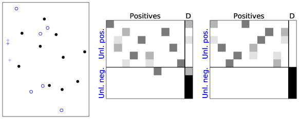
Figure 2: (Left) Positives (black) and Unlabeled (blue) samples (Middle) Transport matrix with no group constraints, where darker color indicates stronger matching (Right) Transport matrix with group constraints.“D” is the dummy point.

Appendix F Standard deviation of accuracy rates of the experiments

Table 3: Standard deviation of accuracy rates on different datasets and scenarios.

Dataset/Scenario	$\pi$	pu	pusb	p-w 0	p-w 0.025	p-gw 0	p-w 0.025
Mushrooms	51.8	0.040	0.047	0.012	0.008	0.008	0.011
Shuttle	78.6	0.032	0.045	0.009	0.012	0.018	0.017
Pageblocks	89.8	0.012	0.010	0.014	0.007	0.012	0.010
USPS	16.7	0.012	0.014	0.004	0.006	0.020	0.021
Connect-4	65.8	0.003	0.010	0.017	0.016	0.019	0.017
Spambase	39.4	0.036	0.039	0.026	0.023	0.022	0.021
Original mnist	10	0.005	0.005	0.005	0.004	0.004	0.01
Colored mnist	10	0.035	0.034	0.004	0.006	0.008	0.012
surf c$\rightarrow$surf c	10	0.019	0.015	0.017	0.014	0.015	0.017
surf c$\rightarrow$surf a	10	0.014	0.018	0.012	0.014	0.018	0.016
surf c$\rightarrow$surf w	10	0.010	0.064	0.014	0.013	0.016	0.010
surf c$\rightarrow$surf d	10	0.006	0.036	0.000	0.000	0.022	0.020
decaf c$\rightarrow$decaf c	10	0.022	0.017	0.013	0.016	0.013	0.009
decaf c$\rightarrow$decaf a	10	0.019	0.022	0.006	0.006	0.004	0.014
decaf c$\rightarrow$decaf w	10	0.030	0.009	0.006	0.006	0.014
decaf c$\rightarrow$decaf d	10	0.033	0.008	0.010	0.009	0.015	0.003
surf c$\rightarrow$decaf c	10	-	-	-	-	0.012	0.013
surf c$\rightarrow$decaf a	10	-	-	-	-	0.011	0.011
surf c$\rightarrow$decaf w	10	-	-	-	-	0.006	006
surf c$\rightarrow$decaf d	10	-	-	-	-	0.010	0.010
decaf c$\rightarrow$surf c	10	-	-	-	-	0.024	0.024
decaf c$\rightarrow$surf a	10	-	-	-	-	0.037	0.037
decaf c$\rightarrow$surf w	10	-	-	-	-	0.022	0.022
decaf c$\rightarrow$surf d	10	-	-	-	-	0.013	0.013

References

• Arjovsky et al. (2019) Arjovsky, M., L. Bottou, I. Gulrajani, and D. Lopez-Paz (2019). Invariant risk minimization. arXiv preprint arXiv:1907.02893.
• Arjovsky et al. (2017) Arjovsky, M., S. Chintala, and L. Bottou (2017). Wasserstein Generative Adversarial Networks. In Proceedings of the 34th International Conference on Machine Learning, Volume 70, pp.  214–223.
• Bekker and Davis (2018) Bekker, J. and J. Davis (2018). Learning from positive and unlabeled data under the selected at random assumption. In Proceedings of Machine Learning Research, Volume 94, pp. 8–22.
• Bekker and Davis (2020) Bekker, J. and J. Davis (2020). Learning from positive and unlabeled data: A survey. Machine Learning 109(719-760).
• Benamou et al. (2015) Benamou, J. D., G. Carlier, M. Cuturi, L. Nenna, and G. Peyré (2015). Iterative Bregman projections for regularized transportation problems. SIAM J. Scientific Computing 37.
• Bonneel and Coeurjolly (2019) Bonneel, N. and D. Coeurjolly (2019). Spot: sliced partial optimal transport. ACM Transactions on Graphics (TOG) 38(4), 1–13.
• Bonneel et al. (2011) Bonneel, N., M. Van de Panne, S. Paris, and W. Heidrich (2011). Displacement interpolation using lagrangian mass transport. ACM Trans. Graph. 30(6), 158:1–12.
• Brécheteau (2019) Brécheteau, C. (2019). A statistical test of isomorphism between metric-measure spaces using the distance-to-a-measure signature. Electronic Journal of Statistics 13(1), 795–849.
• Caffarelli and McCann (2010) Caffarelli, L. A. and R. J. McCann (2010). Free boundaries in optimal transport and monge-ampère obstacle problems. Annals of Mathematics 171(2), 673–730.
• Chizat et al. (2018) Chizat, L., G. Peyré, B. Schmitzer, and F.-X. Vialard (2018). Scaling algorithms for unbalanced optimal transport problems. Math. Comput. 87, 2563–2609.
• Courty et al. (2017) Courty, N., R. Flamary, D. Tuia, and A. Rakotomamonjy (2017). Optimal transport for domain adaptation. IEEE transactions on pattern analysis and machine intelligence 39(9), 1853–1865.
• Cuturi (2013) Cuturi, M. (2013). Sinkhorn distances: Lightspeed computation of optimal transport. In Advances in Neural Information Processing Systems 26, pp. 2292–2300.
• Demyanov and Rubinov (1970) Demyanov, V. F. and A. M. Rubinov (1970). Approximate methods in optimization problems. Elsevier Publishing Company 53.
• Donahue et al. (2014) Donahue, J., Y. Jia, O. Vinyals, J. Hoffman, N. Zhang, E. Tzeng, and T. Darrell (2014). Decaf: A deep convolutional activation feature for generic visual recognition. In International conference on machine learning, pp. 647–655.
• Du Plessis et al. (2014) Du Plessis, M., G. Niu, and M. Sugiyama (2014). Analysis of learning from positive and unlabeled data. In Advances in neural information processing systems, pp. 703–711.
• Elkan and Noto (2008) Elkan, C. and K. Noto (2008). Learning classifiers from only positive and unlabeled data. In Proceedings of the 14th ACM SIGKDD international conference on Knowledge discovery and data mining, pp.  213–220.
• Ferradans et al. (2013) Ferradans, S., N. Papadakis, J. Rabin, G. Peyré, and J. F. Aujol (2013). Regularized discrete optimal transport. In A. Kuijper, K. Bredies, T. Pock, and H. Bischof (Eds.), Scale Space and Variational Methods in Computer Vision, Berlin, Heidelberg, pp. 428–439. Springer Berlin Heidelberg.
• Figalli (2010) Figalli, A. (2010). The optimal partial transport problem. Archive for Rational Mechanics and Analysis 195(2), 533–560.
• Flamary and Courty (2017) Flamary, R. and N. Courty (2017). Pot python optimal transport library. https://github.com/rflamary/POT.
• Frank and Wolfe (1956) Frank, M. and P. Wolfe (1956). An algorithm for quadratic programming. Naval Research Logistics Quarterly 3(1-2), 95–110.
• Griffin et al. (2007) Griffin, G., A. Holub, and P. Perona (2007). Caltech-256 object category dataset. Technical report, California Institute of Technology.
• Guittet (2002) Guittet, K. (2002). Extended kantorovich norms: a tool for optimization. Tech. Rep. 4402.
• Ho et al. (2017) Ho, N., X. L. Nguyen, M. Yurochkin, H. H. Bui, V. Huynh, and D. Phung (2017). Multilevel clustering via wasserstein means. In Proceedings of the 34th International Conference on Machine Learning - Volume 70, pp.  1501–1509.
• Hsieh et al. (2019) Hsieh, Y., G. Niu, and M. Sugiyama (2019). Classification from positive, unlabeled and biased negative data. In Proceedings of the 36th International Conference on Machine Learning, Volume 97.
• Jaggi (2013) Jaggi, M. (2013). Revisiting Frank-Wolfe: Projection-free sparse convex optimization. In Proceedings of the 30th International Conference on Machine Learning, Number 1, pp.  427–435.
• Kato et al. (2019) Kato, M., T. Teshima, and J. Honda (2019). Learning from positive and unlabeled data with a selection bias. In ICLR.
• Kriege and Mutzel (2012) Kriege, N. and P. Mutzel (2012). Subgraph matching kernels for attributed graphs. In Proceedings of the 29th International Conference on Machine Learning.
• Lacoste-Julien (2016) Lacoste-Julien, S. (2016). Convergence rate of Frank-Wolfe for non-convex objectives. CoRR abs/1607.00345.
• Lacoste-Julien and Jaggi (2015) Lacoste-Julien, S. and M. Jaggi (2015). On the global linear convergence of frank-wolfe optimization variants. Neural Information Processing Systems 2015, 496–504.
• Lee et al. (2019) Lee, J., N. Bertrand, and C. Rozell (2019). Parallel unbalanced optimal transport regularization for large scale imaging problems. Technical report, arXiv preprint arXiv:1909.00149. Under review.
• Mémoli (2011) Mémoli, F. (2011). Gromov–Wasserstein distances and the metric approach to object matching. Foundations of Computational Mathematics 11(4), 417–487.
• Peyré and Cuturi (2019) Peyré, G. and M. Cuturi (2019). Computational optimal transport. Foundations and Trends® in Machine Learning 11(5-6), 355–607.
• Peyré et al. (2016) Peyré, G., M. Cuturi, and J. Solomon (2016). Gromov-Wasserstein averaging of kernel and distance matrices. In Proceedings of the 33rd International Conference on International Conference on Machine Learning - Volume 48, pp.  2664–2672.
• Plessis et al. (2017) Plessis, M. C., G. Niu, and M. Sugiyama (2017, April). Class-prior estimation for learning from positive and unlabeled data. Mach. Learn. 106(4), 463–492.
• Ramaswamy et al. (2016) Ramaswamy, H., C. Scott, and A. Tewari (2016). Mixture proportion estimation via kernel embeddings of distributions. In International Conference on Machine Learning, pp. 2052–2060.
• Saenko et al. (2010) Saenko, K., B. Kulis, M. Fritz, and T. Darrell (2010). Adapting visual category models to new domains. In European conference on computer vision, pp.  213–226.
• Solomon et al. (2015) Solomon, J., F. de Goes, G. Peyré, M. Cuturi, A. Butscher, A. Nguyen, T. Du, and L. Guibas (2015). Convolutional wasserstein distances: Efficient optimal transportation on geometric domains. ACM Trans. Graph. 34(4), 66:1–66:11.
• Sturm (2006) Sturm, K. T. (2006). On the geometry of metric measure spaces. Acta Math. 196(1), 133–177.
• Vayer et al. (2018) Vayer, T., L. Chapel, R. Flamary, R. Tavenard, and N. Courty (2018). Fused gromov-wasserstein distance for structured objects: theoretical foundations and mathematical properties. CoRR abs/1811.02834.
• Vayer et al. (2019) Vayer, T., R. Flamary, R. Tavenard, L. Chapel, and N. Courty (2019). Sliced gromov-wasserstein. In Advances in Neural Information Processing Systems 32, pp. 14726–14736. Curran Associates, Inc.
• Villani (2009) Villani, C. (2009). Optimal Transport: Old and New, Volume 338. Springer Berlin Heidelberg.
• Yang and Uhler (2019) Yang, K. D. and C. Uhler (2019). Scalable unbalanced optimal transport using generative adversarial networks. In International Conference on Learning Representations.
• Zhao et al. (2011) Zhao, Y., X. Kong, and S. Philip (2011). Positive and unlabeled learning for graph classification. In 2011 IEEE 11th International Conference on Data Mining, pp. 962–971. IEEE.