Faster uphill relaxation in thermodynamically equidistant temperature quenches

Abstract

We uncover an unforeseen asymmetry in relaxation – for a pair of thermodynamically equidistant temperature quenches, one from a lower and the other from a higher temperature, the relaxation at the ambient temperature is faster in case of the former. We demonstrate this finding on hand of two exactly solvable many-body systems relevant in the context of single-molecule and tracer-particle dynamics. We prove that near stable minima and for all quadratic energy landscapes it is a general phenomenon that also exists in a class of non-Markovian observables probed in single-molecule and particle-tracking experiments. The asymmetry is a general feature of reversible overdamped diffusive systems with smooth single-well potentials and occurs in multi-well landscapes when quenches disturb predominantly intra-well equilibria. Our findings may be relevant for the optimization of stochastic heat engines.

Relaxation processes are a paradigm for condensed matter [1, 2], single-molecule experiments [3] and tracer-particle transport in complex media [4, 5, 6, 7, 8]. Relaxation close to equilibrium was described by the mechanical Onsager-Casimir [9, 10] and thermal Kubo-Yokota-Nakajima [11] linear laws. These pioneering ideas were consistently generalized in numerous ways, most notably, to thermodynamics along individual stochastic trajectories driven far from equilibrium at weak [12, 13] and strong [14, 15, 16, 17, 18] coupling with the bath, anomalous diffusion phenomena [19, 20, 21, 22], and the so-called ’frenesis’ focusing on the dynamical activity – a dynamic counterpart to changes in entropy [23, 24]. Many of these new concepts have been verified by and/or successfully applied in experiments in colloidal systems [25, 26, 27] and single-molecule experiments on nucleic acids [28, 29, 30] and larger biomolecular machines [31].

Not as much is known about transients, in particular those evolving from non-stationary initial conditions. Our present understanding of thermodynamics and in particular the kinetics in transient systems, reversible as well as irreversible, is mostly limited to small deviations from equilibrium [9, 10], non-equilibrium steady states [32, 33, 23, 34, 35], and statistics of the ’house-keeping’ heat [36, 37] and entropy production [38]. The rôle of initial conditions in relaxation was recently studied in the context of the ’Mpemba effect’ – the phenomenon where a hot system can cool down faster than the same system initiated at a lower temperature [39, 40]. Notable recent advances include an information-theoretic bound on the entropy production during relaxation far from equilibrium [41] and a spectral duality between relaxation and first passage processes [42, 43].

It is meanwhile possible to probe the transient, non-equilibrium dynamics of colloids and single molecules, e.g. by temperature-modulated particle tracking [4], time-[44] and temperature-modulated [45], temperature-jump [46] and holographic [47] optical tweezers as well as optical pushing [48]. These experiments allow for systematic investigations of the dependence of relaxation on the direction of the displacement from equilibrium, which is the central question of the present Letter.

Notwithstanding, the dependence of relaxation on the direction of the displacement from equilibrium (see Fig.1) remains elusive. Moreover, as a result of the projection to a lower-dimensional subspace it is expected that observables in many experiments, in particular those tracking individual particles [4] and single-molecules [46, 47], relax in a manner that is not Markovian [8].

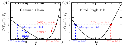
Figure 1: Non-equilibrium free energy after a temperature quench $T\to T_{\mathrm{eq}}$ at time $t=0$ in units of $k_{\mathrm{B}}T_{\mathrm{eq}}$, $\Delta F_{\tilde{T}}=\mathcal{D}[\mathcal{P}_{\tilde{T}}(t=0^{+})||\mathcal{P}^{\mathrm{eq}}_{1}]$ (see Eq. (3)), as a function of the relative pre-quench temperature $\tilde{T}=T/T_{\mathrm{eq}}$ (note the logarithmic scale); a) refers to the end-to-end distance of a Gaussian chain with 100 beads and b) to the 7-th in a single file of 10 particles in a linear potential with slope 10 confined to a unit box. The blue and red points depict a pair of thermodynamically equidistant temperature quenches, $\tilde{T}^{-},\tilde{T}^{+}$, with corresponding excess potential energies $\langle\Delta U\rangle_{\tilde{T}^{\pm}}\equiv\langle U(0^{+})\rangle_{\tilde{T}^{\pm}}-\langle U\rangle_{1}$.

Here, we address relaxation from an instantaneous temperature quench $T\to T_{\mathrm{eq}}$ at time $t=0$ with respect to its directionality, $T^{-}\uparrow T_{\mathrm{eq}}$ versus $T^{+}\downarrow T_{\mathrm{eq}}$. We uncover an unforeseen dependence on the direction of the quench – for a given pair of temperatures $T^{-}<T_{\mathrm{eq}}<T^{+}$ at which the thermodynamic displacement from equilibrium at $t=0^{+}$ in the sense of $\mathcal{D}_{T^{\pm}}(0^{+})$ – the non-equilibrium free energy difference or ’lag’ [49, 50, 51, 52, 53, 54, 55]– is equal, i.e. $\mathcal{D}_{T^{+}}(0^{+})=\mathcal{D}_{T^{-}}(0^{+})$ (see Fig. 1), relaxation evolves, contrary to intuition, faster ’uphill’ ($\langle\Delta U\rangle_{T^{-}}<0$) than ’downhill’ ($\langle\Delta U\rangle_{T^{+}}>0$) the energy landscape. This always holds for single-well potentials and occurs in near degenerate multi-well potentials with high energy barriers, under Markovian dynamics as well as for a class of non-Markovian observables probed by single-molecule and particle-tracking experiments. We demonstrate the asymmetry on hand of the Gaussian polymer chain [56], single-file diffusion in a tilted box [8] and for diffusion in nearly degenerate multi-well potentials. For relaxation near a stable minimum and thus for all reversible Ornstein-Uhlenbeck processes we prove that the asymmetry, albeit counter-intuitive, is general.

Theory.— We consider $d$-dimensional Markovian diffusion with a $d\times d$ symmetric positive-definite diffusion matrix $\mathbf{D}$ and mobility tensor $\mathbf{M}_{T}=\mathbf{D}/k_{\mathrm{B}}T$ in a drift field $\mathbf{F}(\mathbf{x})$ such that $\mathbf{M}_{T}^{-1}\mathbf{F}(\mathbf{x})=-\nabla U(\mathbf{x})$ is a gradient flow. The evolution of the probability density at temperature $T$ is governed by the Fokker-Planck operator $\hat{\mathcal{L}}_{T}\equiv\nabla\cdot\mathbf{D}\nabla-\nabla\cdot\mathbf{M}_{T}\mathbf{F}(\mathbf{x})$. We let $G_{T}(\mathbf{x},t|\mathbf{x}_{0})$ be the Green’s function of the initial value problem $(\partial_{t}-\hat{\mathcal{L}}_{T})G_{T}(\mathbf{x},t|\mathbf{x}_{0})=0$, and assume that the potential $U(\mathbf{x})$ is confining (i.e. $\lim_{|\mathbf{x}|\to\infty}U(\mathbf{x})=\infty$). This assures the existence of an invariant Maxwell-Boltzmann measure with density $\lim_{t\to\infty}G_{T}(\mathbf{x},t|\mathbf{x}_{0})\equiv P_{T}^{\mathrm{eq}}(\mathbf{x})=Q_{T}^{-1}\mathrm{e}^{-U(\mathbf{x})/k_{\mathrm{B}}T},\forall\mathbf{x}_{0}$ with partition function $Q_{T}=\int\mathrm{e}^{-U(\mathbf{x})/k_{\mathrm{B}}T}d\mathbf{x}$.

The system is prepared at equilibrium with a temperature $T$, $P_{T}^{\mathrm{inv}}(\mathbf{x})$, whereupon an instantaneous temperature quench is performed to the ambient temperature $T_{\mathrm{eq}}$ at $t=0$. The relaxation evolves at $T_{\mathrm{eq}}$ according to $\hat{\mathcal{L}}_{T_{\mathrm{eq}}}$ and for a given system it is uniquely characterized by $T$. For convenience we define $\tilde{T}\equiv T/T_{\mathrm{eq}}$ , such that

$$P_{\tilde{T}}(\mathbf{x},t)=\!\int\!\!d\mathbf{x}_{0}G_{1}(\mathbf{x},t|\mathbf{x}_{0})P_{\tilde{T}}^{\mathrm{eq}}(\mathbf{x}_{0})\xrightarrow[t\to\infty]{}P_{1}^{\mathrm{eq}}(\mathbf{x}).$$ (1)

The instantaneous entropy and mean energy are given by $S_{\tilde{T}}(t)\equiv-k_{\mathrm{B}}\int d\mathbf{x}P_{\tilde{T}}(\mathbf{x},t)\ln P_{\tilde{T}}(\mathbf{x},t)$ and $\langle U(t)\rangle_{\tilde{T}}=\int d\mathbf{x}P_{\tilde{T}}(\mathbf{x},t)U(\mathbf{x})$, respectively, where $\langle\cdot\rangle_{\tilde{T}}$ denotes an average over all paths $\mathbf{x}(t)$ starting from $P_{\tilde{T}}^{\mathrm{inv}}(\mathbf{x}_{0})$.

Let the measured physical observable be $\mathbf{q}=\bm{\Gamma}(\mathbf{x})$. Its probability density function corresponds to [8]

$$\mathcal{P}_{\tilde{T}}(\mathbf{q},t)=\hat{\Pi}_{\mathbf{x}}(\mathbf{q})P_{\tilde{T}}(\mathbf{x},t)\!\equiv\!\!\int\!\!d\mathbf{x}\delta(\bm{\Gamma}(\mathbf{x})-\mathbf{q})P_{\tilde{T}}(\mathbf{x},t),$$ (2)

which in general displays non-Markovian dynamics as soon as $\mathbf{q}$ corresponds to a low-dimensional projection [8]. Once equilibrium is reached we have $\lim_{t\to\infty}\mathcal{P}_{\tilde{T}}(\mathbf{q},t)=\mathcal{P}^{\mathrm{eq}}_{1}(\mathbf{q})$, or, expressed via the so-called potential of mean force $\mathcal{U}(\mathbf{q})$ , $\mathcal{P}^{\mathrm{eq}}_{1}(\mathbf{q})=\mathrm{e}^{-\beta_{\mathrm{eq}}\mathcal{U}(\mathbf{q})}$ [59, 14, 17]. Obviously, when $\bm{\Gamma}(\mathbf{x})=\mathbf{x}$ we have $\mathcal{P}_{\tilde{T}}(\mathbf{q},t)=P_{\tilde{T}}(\mathbf{x},t)$.

We quantify the instantaneous displacement from equilibrium with the Kullback-Leibler divergence [49, 50, 51, 52, 53, 54, 55]

$$\mathcal{D}[\mathcal{P}_{\tilde{T}}(t)||\mathcal{P}^{\mathrm{eq}}_{1}]=\int d\mathbf{q}\mathcal{P}_{\tilde{T}}(\mathbf{q},t)\ln(\mathcal{P}_{\tilde{T}}(\mathbf{q},t)/\mathcal{P}^{\mathrm{eq}}_{1}(\mathbf{q})).$$ (3)

Writing this out for the Markovian case we find, upon identifying $S_{\tilde{T}}(t)$ and $\langle U_{\tilde{T}}(t)\rangle$

$$\mathcal{D}[P_{\tilde{T}}(t)||P^{\mathrm{eq}}_{1}]=-S_{\tilde{T}}(t)/k_{\mathrm{B}}+\beta_{\mathrm{eq}}\langle U(t)\rangle_{\tilde{T}}+\ln Q_{T_{\mathrm{eq}}}.$$ (4)

Recalling the definition of free energy $F=-\beta_{\mathrm{eq}}^{-1}\ln Q_{T_{\mathrm{eq}}}$ and defining the instantaneous generalized free energy (GFE) [52] or ’lag’ [55] as $F_{\tilde{T}}(t)=\langle U(t)\rangle_{\tilde{T}}-T_{\mathrm{eq}}S_{\tilde{T}}(t)$ we see, upon multiplying through by $\beta_{\mathrm{eq}}^{-1}=k_{\mathrm{B}}T_{\mathrm{eq}}$, that in the Markovian case Eq. (3) is the excess GFE in units of $k_{\mathrm{B}}T_{\mathrm{eq}}$, i.e. $\mathcal{D}_{\tilde{T}}^{M}(t)\equiv\mathcal{D}[P_{\tilde{T}}(t)||P_{1}^{\mathrm{eq}}]=\beta_{\mathrm{eq}}(F_{\tilde{T}}(t)-F)$ [51, 52]. Writing out Eq. (3) for the non-Markovian case and identifying $\mathcal{S}_{\tilde{T}}(t)$ and $\mathcal{U}(\mathbf{q})$ (calligraphic letters denote potentials of projected observables) we find

$$\mathcal{D}_{\tilde{T}}^{nM}(t)\equiv\mathcal{D}[\mathcal{P}_{\tilde{T}}(t)||\mathcal{P}_{1}^{\mathrm{eq}}]=\!\!-\mathcal{S}_{\tilde{T}}(t)/k_{\mathrm{B}}+\beta_{\mathrm{eq}}\langle\mathcal{U}(t)\rangle_{\tilde{T}},$$ (5)

which is the non-Markovian GFE, $\mathcal{D}_{\tilde{T}}^{nM}(t)=\beta_{\mathrm{eq}}\mathcal{F}_{\tilde{T}}(t)$. Note that $\mathcal{U}(\mathbf{q})$ itself is an effective free energy, i.e. $\beta_{\mathrm{eq}}\mathcal{U}(\mathbf{q})\equiv-\ln\langle\delta(\bm{\Gamma}(\mathbf{x})-\mathbf{q})\rangle_{1}=-\ln\int d\mathbf{x}\delta(\bm{\Gamma}(\mathbf{x})-\mathbf{q})\mathrm{e}^{-\beta_{\mathrm{eq}}U(\mathbf{x})}+\ln Q_{T_{\mathrm{eq}}}$ and $\mathcal{S}_{1}=-\langle\mathcal{U}\rangle_{1}$. We henceforth express energies in units of $k_{\mathrm{B}}T_{\mathrm{eq}}$. If (and only if) latent degrees of freedom (i.e. those integrated out) relax much faster than $\mathbf{q}(t)$, Eqs. (4) and (5) are equivalent and $\mathbf{q}(t)$ is a Markovian diffusion in the free energy landscape $\mathcal{U}(\mathbf{q})$ [8]. In absence of a time-scale separation, however, both $\mathcal{S}_{\tilde{T}}(t)$ and $\langle\mathcal{U}(t)\rangle_{\tilde{T}}$ contain contributions from the (hidden) relaxation of the latent degrees of freedom.

Consider now a pair of temperatures $\tilde{T}^{+}>1$ and $\tilde{T}^{-}<1$ corresponding to equal displacements immediately after the quench: $\mathcal{D}^{M,nM}_{\tilde{T}^{-}}(0^{+})=\mathcal{D}^{M,nM}_{\tilde{T}^{+}}(0^{+})$. The existence of (at least) two such temperatures is guaranteed within an interval $\tilde{T}\in(\tilde{T}_{\mathrm{min}},\tilde{T}_{\mathrm{max}})$ where $\mathcal{D}^{M,nM}_{\tilde{T}}(0^{-})=f(\tilde{T})$ has no local maximum. The central question of this Letter addresses the rate of the ’uphill’ ($\tilde{T}^{-}<1$) versus ’downhill’ ($\tilde{T}^{+}>1$) relaxation.

Gaussian Chain.— In the context of single-molecule experiments we consider the overdamped dynamics of a chain of $N+1$ beads with coordinates $\{\mathbf{r}_{i}\}$ connected by harmonic springs with potential $U(\{\mathbf{r}_{i}\})=\sum_{i=1}^{N}(\mathbf{r}_{i+1}-\mathbf{r}_{i})^{2}$ (general harmonic networks are treated in the SM). In the Markovian setting we consider all monomers, $P_{\tilde{T}}(\{\mathbf{r}_{i}\},t)$ in Eq. (1), while single-molecule experiments (e.g. FRET [60, 61] or optical tweezers [46, 47]) typically track a single (e.g end-to-end) distance within the macromolecule, $\mathbf{q}\equiv d=|\mathbf{r}_{1}-\mathbf{r}_{N}|$ with $\mathcal{P}_{\tilde{T}}(d,t)$ from Eq. (2), evolving according to non-Markovian dynamics.

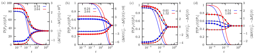
Figure 2: $\mathcal{D}[\mathcal{P}_{\tilde{T}}(t)||\mathcal{P}^{\mathrm{eq}}_{1}]$ (full lines) for the Gaussian chain (a and b) and single-file with 10 particles in a linear potential with slope $g=10$ (s and d). a) refers to the entire chain of 100 beads (Eq. (4)) and b) to the end-to-end distance (Eq. (5)) for equidistant quenches from $\tilde{T}^{-}=0.24$ (blue) and $\tilde{T}^{+}=2.64$ (red); c) stands for the full single file for equidistant quenches from $\tilde{T}^{-}=0.61$ (blue) and $\tilde{T}^{+}=1.52$ (red); d) the 7-th particle for equidistant quenches from $\tilde{T}^{-}=0.54$ (blue) and $\tilde{T}^{+}=1.69$. The circles refer to $\langle\Delta U(t)\rangle_{\tilde{T}^{\pm}}$ and $\langle\Delta\mathcal{U}(t)\rangle_{\tilde{T}^{\pm}}$ in a and c, and b and d, respectively, and triangles denote $\Delta S_{\tilde{T}^{\pm}}(t)$ and $\Delta\mathcal{S}_{\tilde{T}}(t)$. Note the second axes for $\langle\Delta U(t)\rangle_{\tilde{T}^{\pm}},\langle\Delta\mathcal{U}(t)\rangle_{\tilde{T}^{\pm}}$ and $\Delta S_{\tilde{T}^{\pm}}(t),\Delta\mathcal{S}_{\tilde{T}}(t)$. Note that $\mathcal{S}_{\tilde{T}}(\infty)=\mathcal{S}_{1}=-\langle\mathcal{U}\rangle_{1}$.

The excess GFE is given by (see derivation in the SM)

$$\mathcal{D}^{M}_{\tilde{T}}(t) = \frac{3}{2}\sum_{k=1}^{N}\left[\Lambda_{k}^{\tilde{T}}(t)-1-\ln\Lambda_{k}^{\tilde{T}}(t)\right]$$ (6)

$$\mathcal{D}_{\tilde{T}}^{nM}(t) = \frac{3}{2}\left[\frac{\mathcal{A}_{\tilde{T}}^{1N}(t)}{\mathcal{A}_{1}^{1N}(0)}-1-\ln\frac{\mathcal{A}_{\tilde{T}}^{1N}(t)}{\mathcal{A}^{1N}_{1}(0)}\right],$$ (7)

where $\Lambda_{k}^{\tilde{T}}(t)\equiv 1+(\tilde{T}-1)\mathrm{e}^{-2\mu_{k}t}$ with $\mu_{k}=4\sin^{2}(\frac{k\pi}{2(N+1)})$ and we introduced $\mathcal{A}_{\tilde{T}}^{ij}(t)\equiv\sum_{k=1}^{N}\Lambda_{k}^{\tilde{T}}(t)\mathcal{C}_{k}^{ij}/2\mu_{k}$ with $\mathcal{C}_{k}^{ij}\geq 0$ given explicitly in the SM. The initial excess free energies are both convex in $\tilde{T}$ and read

$$\mathcal{D}_{\tilde{T}}^{M}(0^{+})=3N(\tilde{T}-1-\ln\tilde{T})/2=N\mathcal{D}_{\tilde{T}}^{nM}(0^{+}).$$ (8)

The instantaneous potential energy of the full system and the potential of mean force in turn read $\langle U(t)\rangle_{\tilde{T}}=\frac{3}{2}\sum_{k=1}^{N}\Lambda_{k}^{\tilde{T}}(t)$ and $\mathcal{U}(d)=-\ln\mathcal{P}_{1}^{\mathrm{eq}}(d)$, respectively. Aside from specific values of $\mu_{k}$ and $\mathcal{C}^{ij}_{k}$ Eqs. (6-8) hold for any reversible Ornstein-Uhlenbeck process, that is for any $\tilde{T}$, connectivity/topology, and tagged distance.

The results for $\mathcal{D}_{\tilde{T}}^{M,nM}(t)$ and their decomposition into $\langle U\rangle_{\tilde{T}},\langle\mathcal{U}(t)\rangle_{\tilde{T}},S_{\tilde{T}}(t),$ and $\mathcal{S}_{\tilde{T}}(t)$ for a pair of equidistant temperature quenches are shown in Fig. 2 and demonstrate that the uphill relaxation is always faster than downhill relaxation. As we prove below this is true for any reversible Ornstein-Uhlenbeck process (OUp) quenched arbitrarily far from equilibrium.

The energy and entropy differences relative to their equilibrium values (i.e. at $t=\infty$) in Fig. 2a suggest that the Markovian uphill and downhill relaxation are dominated by $\langle\Delta U(t)\rangle_{\tilde{T}^{+}}$ and $\Delta S_{\tilde{T}^{-}}$, respectively. Surprisingly, entropy pushing the system uphill against the deterministic force is more efficient. Notably, the magnitude of individual contributions is smaller for uphill relaxation, i.e. $\langle\Delta U\rangle_{\tilde{T}^{+}}>-\langle\Delta U\rangle_{\tilde{T}^{-}}$ and $\Delta S_{\tilde{T}^{+}}>-\Delta S_{\tilde{T}^{-}}$. Thus, a larger energy excess and entropy deficit are dissipated during downhill relaxation. Conversely, the partitioning into $\mathcal{S}_{\tilde{T}}(t)$ and $\langle\mathcal{U}(t)\rangle_{\tilde{T}}$ of the non-Markovian relaxation depends on the details of the projection and is less intuitive (in our example in Fig. 2b it is in fact reversed).

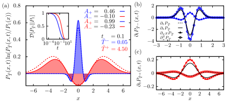
Figure 3: a) Integrand of Eq. (3) at $t=0.1$ for a one-dimensional OUp (full line) for uphill (blue) and downhill (red) relaxation with the positive $A_{+}$ and negative $A_{-}$ area under the curve; Inset: The corresponding $\mathcal{D}_{\tilde{T}}^{M}(t)$. b-c) Decomposition of $\partial_{t}P_{\tilde{T}}(x,t)$ into diffusive $\partial^{2}_{x}P_{\tilde{T}}$ (circles) and advective $\partial_{x}xP_{\tilde{T}}$ (triangles) contribution for uphill (b) and downhill (c) relaxation. Dashed lines correspond to free diffusion evolving from the same initial condition.

To explain why uphill relaxation is faster we inspect in Fig. 3 local contributions to $\mathcal{D}_{\tilde{T}}^{M}(t)$ for a one-dimensional OUp. An uphill quench localizes $P_{\tilde{T}^{-}}(x,0^{+})$ near the origin, whereas a downhill quench broadens $P_{\tilde{T}^{+}}(x,0^{+})$ rendering the integrand of Eq. (4) non-zero over a larger domain (Fig. 3a, red line). The evolution of $P_{\tilde{T}}(x,t)$ is driven by diffusion $\propto\partial^{2}_{x}P_{\tilde{T}}$ and advection $\propto\partial_{x}xP_{\tilde{T}}$. By forcing probability mass towards the origin advection seems to oppose uphill relaxation (triangles in Fig. 3b) but thereby actually sustains an even faster diffusion rate compared to free diffusion (compare circles and dashed line in Fig. 3b). The net effect is an overall relaxation nearly as fast as free diffusion (compare full and dashed line in Fig. 3b). Downhill relaxation is advection-dominated and weakly opposed by diffusion, which is almost unaffected by the potential (Fig. 3c). The overall dynamics is much slower (compare full lines in Fig. 3b & c). Faster diffusion from a localized initial distribution thereby renders uphill relaxation faster – an effect that will exist in any confining potential well with ruggedness $\ll k_{\rm B}T_{\mathrm{eq}}$. $\hat{\mathcal{L}}_{T}$ of any reversible OUp is diagonalizable and thus uniquely decomposable into one-dimensional OUps, extending our explanation to arbitrary dimensions.

Non-Markovian relaxation displays the same asymmetry but the dominant driving forces, here $\mathcal{S}_{\tilde{T}}$ and $\langle\mathcal{U}_{\tilde{T}}\rangle$, may become reversed (see Fig. 2b). Since $\mathcal{U}_{\tilde{T}}$ contains entropic effects of latent degrees of freedom the partitioning between $\mathcal{S}_{\tilde{T}}$ and $\langle\mathcal{U}_{\tilde{T}}\rangle$ is in general projection-dependent.

Tilted Single File.— In the context of tracer-particle dynamics we consider $N$ hard-core Brownian point particles with positions $\{x_{i}(t)\}$ (the extension to a finite diameter is straightforward [6, 5]) diffusing in a box of unit length in the presence of a linear potential (e.g. the gravitational field), $U(\{x_{i}\})=\sum_{i=1}^{N}gx_{i}$. The probability density of $\{x_{i}(t)\}$ upon a quench from $\tilde{T}$, $P_{\tilde{T}}(\{x_{i}(t)\},t)$, evolves according to $\hat{\mathcal{L}}_{1}=\sum_{i=1}^{N}(\partial_{x_{i}}^{2}+g\partial_{x_{i}})$ under non-crossing conditions [7, 8]. In the SM we solve the problem exactly via the coordinate Bethe ansatz [7, 8], both for the Markovian complete single file and the non-Markovian probability density of a tagged particle $\mathcal{P}_{\tilde{T}}(z,t)$ (i.e. $\mathbf{q}\equiv x_{\mathcal{T}}=z$).

$\mathcal{D}^{M}_{\tilde{T}}(t)$ with corresponding $\langle\Delta U(t)\rangle_{\tilde{T}},\langle\mathcal{U}(t)\rangle_{\tilde{T}},\Delta S_{\tilde{T}}(t)$ and $\mathcal{S}_{\tilde{T}}(t)$ for the complete and tagged particle dynamics are shown in Fig. 2 c and d. As for the Gaussian chain uphill relaxation in the tilted single file, both full as well as for a tagged particle, seems to always be faster, irrespective of which particle we tag and for any $\tilde{T},N$ and tilting strength $g>0$ (see also SM). The Markovian uphill relaxation is dominated by $\Delta S_{\tilde{T}^{-}}(t)$ and downhill by $\langle\Delta U(t)\rangle_{\tilde{T}^{+}}$, and a larger energy and entropy difference must be dissipated during downhill relaxation (see Fig. 2c). For a tagged-particle the partitioning between $\langle\mathcal{U}(t)\rangle_{\tilde{T}^{-}}$ and $\mathcal{S}(t)_{\tilde{T}^{-}}$ varies depending on which particle we tag as a result of the shape of $\mathcal{U}(z)$ and the dependence of $\mathcal{P}_{\tilde{T}}(z,0^{-})$ on $\tilde{T}$, which in turn both depend on the tagged particle as well as $T_{\mathrm{eq}},N$ and $g$.

Is the asymmetry universal?— We first focus on dynamics near a stable minimum at $\mathbf{R}_{0}$, $\delta\mathbf{R}(t)=\mathbf{R}(t)-\mathbf{R}_{0}$, which is well described by an Ornstein-Uhlenbeck process (OUp), i.e. $d\delta\mathbf{R}(t)=\mathrm{\mathbf{H}}\delta\mathbf{R}(t)dt+\sqrt{2}d\mathbf{W}_{t}$, where $(\mathrm{\mathbf{H}})_{ij}=\sum_{ij}\partial_{R_{i}}\partial_{R_{j}}U(\mathbf{R})|_{\mathbf{R}_{0}}$ is the Hessian.

Theorem 1.

For a general diffusion sufficiently close to a stable minimum and for any stable reversible OUp the relaxation from a pair of equidistant quenches of arbitrary magnitude (as defined above) is always faster uphill.

Proof.

(See Erratum) Any pair $0<\tilde{T}^{-}\leq 1$ and $1\leq\tilde{T}^{+}<\infty$ with $\mathcal{D}_{\tilde{T}^{+}}(0^{+})=\mathcal{D}_{\tilde{T}^{-}}(0^{+})$ satisfies by construction $\tilde{T}^{+}-\tilde{T}^{-}=\ln(\tilde{T}^{+}/\tilde{T}^{-})$. We first prove the claim for the Markovian setting, where Eq. (6) has the structure $\mathcal{D}_{\tilde{T}}^{M}(t)=\sum_{k=1}^{N}\mathcal{D}^{\pm}_{k}(t)$. We set $\varphi\equiv\tilde{T}^{+}/\tilde{T}^{-}>1$, $\delta_{\pm}\equiv\tilde{T}^{\pm}-1$, and write $\Delta\mathcal{D}_{k}(t)\equiv\mathcal{D}^{+}_{k}(t)-\mathcal{D}^{-}_{k}(t)=\ln Z_{\varphi}(\mu_{k}t)$, such that

$$Z_{\varphi}(\tau) = \varphi^{\mathrm{e}^{-\tau}}(1+\delta_{-}\mathrm{e}^{-\tau})/(1+\delta_{+}\mathrm{e}^{-\tau})$$ (9)

$$= [\varphi(1+\delta_{-}\mathrm{e}^{-\tau})^{\mathrm{e}^{\tau}}]^{\mathrm{e}^{-\tau}}/(1+\delta_{+}\mathrm{e}^{-\tau})$$

$$\geq [\varphi(1+\delta_{-})/(1+\delta_{+})]^{\mathrm{e}^{-\tau}}\geq 1,$$

where we have used both generalized Bernoulli inequalities, i.e. for any real $0\leq y_{-}\leq 1$, $y_{+}\geq 1$ and $x\geq-1$ we have $(1+x)^{y_{+}}\geq 1+y_{+}x$ and $(1+x)^{y_{-}}\leq 1+y_{-}x$. Recalling the definition of $\Delta\mathcal{D}_{k}(t)$ completes the proof.

To prove the claim in the non-Markovian setting for projections of type $q=|\delta\mathbf{R}_{i}-\delta\mathbf{R}_{j}|$ we first realize that $\dot{\mathcal{A}}_{\tilde{T}^{+}}^{ij}(t)\leq 0$ and $\dot{\mathcal{A}}_{\tilde{T}^{-}}^{ij}(t)\geq 0$, where $\dot{f}(t)\equiv\frac{d}{dt}f(t)$. Setting $\Delta\mathcal{D}(t)\equiv\mathcal{D}^{nM}_{\tilde{T}^{+}}(t)-\mathcal{D}^{nM}_{\tilde{T}^{-}}(t)$ and using Eq.(7) we find, upon taking the derivative

$$\Delta\dot{\mathcal{D}}(t)=\frac{\dot{\mathcal{A}}_{\tilde{T}^{+}}^{ij}(t)}{\mathcal{A}_{\tilde{T}^{+}}^{ij}(0)}-\frac{\dot{\mathcal{A}}_{\tilde{T}^{+}}^{ij}(t)}{\mathcal{A}_{\tilde{T}^{+}}^{ij}(t)}-\frac{\dot{\mathcal{A}}_{\tilde{T}^{-}}^{ij}(t)}{\mathcal{A}_{\tilde{T}^{-}}^{ij}(0)}+\frac{\dot{\mathcal{A}}_{\tilde{T}^{-}}^{ij}(t)}{\mathcal{A}_{\tilde{T}^{-}}^{ij}(t)}.$$ (10)

Eq. (10) implies $\Delta\dot{\mathcal{D}}(t)\geq 0$ because $\mathcal{A}_{\tilde{T}^{+}}^{ij}(t)\geq\mathcal{A}_{\tilde{T}^{+}}^{ij}(0)$ while $\mathcal{A}_{\tilde{T}^{-}}^{ij}(t)\leq\mathcal{A}_{\tilde{T}^{+}}^{ij}(0)$, which completes the proof. ∎

The fact that tilted single-file diffusion, being anharmonic and asymmetric with non-perturbative interactions, displays the asymmetry for quenches of arbitrary magnitude and for any steepness of the potential hints that the asymmetry might be more general. Note that tagging different particles in different slopes $g>0$ we can construct $\mathcal{U}(z)$ with arbitrary asymmetry. Alongside the physical principle underlying the asymmetry established for the OUp and Theorem 1 this strongly suggest that uphill relaxation in smooth single-well potentials could be universally faster (see SM). Since the projection (2) is independent of $\tilde{T}$ these statements should extend also to non-Markovian observables, in particular those probed in many single-molecule and particle-tracking experiments.

As a corollary uphill relaxation is faster also in multi-well potentials for equidistant quenches that predominantly disturb only the intra-well equilibria, in particular for nearly degenerate basins separated by sufficiently high barriers [62] (for reasoning and examples see SM). This is violated in asymmetric multi-wells and examples with faster downhill relaxation are constructed in the SM.

Conclusion.— We uncovered an unforeseen asymmetry in the relaxation to equilibrium in equidistant temperature quenches. Uphill relaxation was found to be faster – a phenomenon we proved to be universal for quenches of dynamics near stable minima. We hypothesize that it is a general phenomenon in reversible overdamped diffusion in single-well potentials extending to degenerate multi-well potentials for quenches leaving inter-well equilibria virtually intact. The dependence on the direction of the quench, which so far seems to have been overlooked, implies a systematic asymmetry in the dissipation of the system’s entropy $\dot{S}_{\tilde{T}}(t)$ versus heat $\langle\dot{U}(t)\rangle_{\tilde{T}}$ [12] and, for specific projections, the modified entropy $\dot{\mathcal{S}}_{\tilde{T}}(t)$ versus ’strong coupling heat’ $\langle\dot{\mathcal{U}}(t)\rangle_{\tilde{T}}$ [14, 17], which seems to be relevant for the efficiency of stochastic heat engines [44, 63, 64]. Implying that the hot isothermal step can be shorter than the cold one, which reduces cycle times, the asymmetry may also be relevant for the optimization of the engine’s output power [44, 63, 64]. Our results can readily be tested by single-molecule and particle-tracking experiments [4, 44, 45, 46, 47, 48]. To understand the asymmetry on the level of individual trajectories it would be interesting to analyze relaxation from equidistant quenches in terms of occupation measures [7, 8] and from the perspective of stochastic thermodynamics [12, 14].

Erratum:
Faster Uphill Relaxation in Thermodynamically Equidistant Temperature Quenches

While Theorem 1 in [1] holds true as stated, the proof of the theorem contains a technical error, i.e. one of the inequalities in Eq. (9) was unfortunately applied in the false direction and there is also an error in Eq. (10), which renders the proof invalid. Most importantly, the statement of Theorem 1 as well as all the results and conclusions of the Letter [1] remain entirely unaffected.

Here we provide a valid proof of Theorem 1, which is slightly longer but straightforward. The present proof covers both cases, Eqs. (9) and (10). We introduce $\Gamma(t)\equiv\sum_{k}[\mathcal{C}_{k}\mathrm{e}^{-2\mu_{k}t}/\mu_{k}]/\sum_{k}[\mathcal{C}_{k}/\mu_{k}]$ such that $0<\Gamma(t)\leq 1$, with the notation $\delta_{\pm}\equiv\tilde{T}_{\pm}-1$ as in [1] we may write for the Markovian, $\Delta\mathcal{D}_{k}(t)$, and non-Markovian, $\Delta\mathcal{D}^{\rm nM}(t)$, setting

$$\Delta\mathcal{D}_{k}(t)=\frac{3}{2}\left[(\delta_{+}-\delta_{-})e^{-2\mu_{k}t}-\ln\left(\frac{1+\delta_{+}e^{-2\mu_{k}t}}{1+\delta_{-}e^{-2\mu_{k}t}}\right)\right],\qquad\Delta\mathcal{D}^{\rm nM}(t)=\frac{3}{2}\left[(\delta_{+}-\delta_{-})\Gamma(t)-\ln\left(\frac{1+\delta_{+}\Gamma(t)}{1+\delta_{-}\Gamma(t)}\right)\right].$$ (E11)

It is to prove that $\Delta\mathcal{D}_{k}(t)\geq 0$ for all $t$. By defining $y\equiv e^{2\mu_{k}t}$ or $y\equiv\Gamma^{-1}(t)$ this is equivalent to showing

$$y\ln\left(\frac{y+\delta_{+}}{y+\delta_{-}}\right)\leq\delta_{+}-\delta_{-}\ .$$ (E12)

for all $y\geq 1$. Since $\delta_{+}\geq 0\geq\delta_{-}>-1$ we have that $x\equiv(y+\delta_{+})/(y+\delta_{-})\geq 1$ and we can further apply that for $x\geq 1$ we have $\ln(x)\leq(x-1)/\sqrt{x}$ [3] to obtain

$$y\ln\left(\frac{y+\delta_{+}}{y+\delta_{-}}\right)\leq y\frac{\frac{y+\delta_{+}}{y+\delta_{-}}-1}{\sqrt{\frac{y+\delta_{+}}{y+\delta_{-}}}}=\frac{\delta_{+}-\delta_{-}}{\sqrt{(1+\delta_{+}/y)(1+\delta_{-}/y)}},$$ (E13)

which allows to conclude Eq. (E12) (and thus completes the proof) for any $y$ with $(1+\delta_{+}/y)(1+\delta_{-}/y)\geq 1$.

For the case $(1+\delta_{+}/y)(1+\delta_{-}/y)\leq 1$ we need a different approach. Here, we write

$$x^{\prime} \equiv 1-\frac{(y+\delta_{+})(1+\delta_{-})}{(y+\delta_{-})(1+\delta_{+})}=\frac{(y+\delta_{-})(1+\delta_{+})-(y+\delta_{+})(1+\delta_{-})}{(y+\delta_{-})(1+\delta_{+})}=\frac{(\delta_{+}-\delta_{-})(y-1)}{(y+\delta_{-})(1+\delta_{+})}\geq 0,$$ (E14)

($x^{\prime}\geq 0$ since $y+\delta_{-}>y-1\geq 0$ and $\delta_{+}-\delta_{-}\geq 0$), such that we can re-write the left hand side of Eq. (E12) as

$$y\ln\left(\frac{y+\delta_{+}}{y+\delta_{-}}\right) =y\ln\left(\frac{(y+\delta_{+})(1+\delta_{-})}{(y+\delta_{-})(1+\delta_{+})}\times\frac{1+\delta_{+}}{1+\delta_{-}}\right)=y\ln(1-x^{\prime})+y\ln\left(\frac{1+\delta_{+}}{1+\delta_{-}}\right)=y\ln(1-x^{\prime})+y(\delta_{+}-\delta_{-}),$$ (E15)

where we used the equidistant quenches condition $\ln\left(\frac{1+\delta_{+}}{1+\delta_{-}}\right)=\delta_{+}-\delta_{-}$. Recall that we are now considering $(1+\delta_{+}/y)(1+\delta_{-}/y)\leq 1$ and thus $\delta_{+}\delta_{-}+y(\delta_{+}+\delta_{-})\leq 0$, and it follows (note that $\tilde{T}_{-}=-W_{0}(-\tilde{T}_{+}\mathrm{e}^{-\tilde{T}_{+}})$ with $W_{0}(z)$ denoting the principal branch of the Lambert-W function [1], and $\delta_{+}+\delta_{-}=\tilde{T}_{+}+\tilde{T}_{-}-2\geq 0$ by Theorem 3.2 in [4])

$$2(y\!+\!\delta_{-})(1\!+\!\delta_{+})\!-\!(\delta_{+}\!-\!\delta_{-})(y-1) =2y-(y-1)(\delta_{+}\!+\!\delta_{-})\!+\!2[\delta_{+}\delta_{-}+y(\delta_{+}\!+\!\delta_{-})]\leq 2y-(y-1)(\delta_{+}+\delta_{-})\leq 2y.$$ (E16)

Applying $\ln(1-x^{\prime})\leq\frac{-2x^{\prime}}{2-x^{\prime}}$ for $0\leq x^{\prime}<1$ [3] ($x^{\prime}<1$ follows from Eq. (E14)) we further obtain, using Eq. (E14) and (E16)

$$y\ln(1-x^{\prime})\leq y\frac{-2x^{\prime}}{2-x^{\prime}}=-2y\frac{(\delta_{+}-\delta_{-})(y-1)}{2(y+\delta_{-})(1+\delta_{+})-(\delta_{+}-\delta_{-})(y-1)}\overset{{\rm Eq.}\leavevmode\nobreak\ \eqref{some ineq}}{\leq}-(\delta_{+}-\delta_{-})(y-1),$$ (E17)

noting that the expressions negative. Plugging this into Eq. (E15) yields Eq. (E12) and thus completes the proof.

Acknowledgments. We thank Cai Dieball for discovering the error, and for his major contribution to finding the shortest and most elegant proof of the theorem.

Abstract

In this Supplementary Material (SM) we present detailed derivations of the main results for the Gaussian-Chain and tilted single-file diffusion model presented in the main Letter, as well as several supplementary examples with figures. We also present counterexamples demonstrating that the uphill-downhill asymmetry is not universal as it vanishes in sufficiently asymmetric multi-well potentials. However, we establish generic conditions under which the asymmetry is obeyed. Finally, we also discuss the non-Markovian Mpemba effect.

I Gaussian Chain and Ornstein-Uhlenbeck process

We consider a Gaussian Chain with N+1 beads with coordinates $\mathbf{R}=\{\mathbf{r}_{i}\}$ connected by harmonic springs with potential energy $U(\mathbf{R})=\frac{1}{2}\sum_{i=1}^{N}|\mathbf{r}_{i}-\mathbf{r}_{i+1}|^{2}$. The overdamped Langevin equation governing the dynamics of a Gaussian Chain with N+1 beads connected by ideal springs with zero rest-length and diffusion coefficient $D$ is given by the set of coupled Itô equations

$$d\mathbf{r}_{1}(t) = [-\mathbf{r}_{1}(t)+\mathbf{r}_{2}(t)]dt+\sqrt{2D}\bm{\xi}_{1}(t)$$

$$d\mathbf{r}_{i}(t) = [\mathbf{r}_{i-1}(t)-2\mathbf{r}_{i}(t)+\mathbf{r}_{i+1}(t)]dt+\sqrt{2D}\bm{\xi}_{i}(t)$$

$$d\mathbf{r}_{N+1}(t) = [-\mathbf{r}_{N+1}(t)+\mathbf{r}_{N}(t)]dt+\sqrt{2D}\bm{\xi}_{N+1}(t),$$ (S1)

where $\bm{\xi}_{i}(t)$ stands for zero mean Gaussian white noise, i.e.

$$\langle\bm{\xi}_{i}(t)\rangle=0,\qquad\langle\xi_{i,k}(t)\xi_{i,l}(t^{\prime})\rangle=\delta_{kl}\delta(t-t^{\prime}).$$ (S2)

It is straightforward to generalize these formulas to any reversible $M$-dimensional Ornstein-Uhlenbeck process $\mathbf{R}(t)\equiv\{\mathbf{r}_{i}(t)\}$ with some $\mathbb{R}^{M}\times\mathbb{R}^{M}$ symmetric force matrix $\bm{\Xi}$ and potential energy function $U(\mathbf{R})=\frac{1}{2}\mathbf{R}^{T}\bm{\Xi}\mathbf{R}$

$$d\mathbf{R}(t)=\bm{\Xi}\mathbf{R}(t)dt+\sqrt{2}d\mathbf{W}_{t},$$ (S3)

where $d\mathbf{W}_{t}$ is the $M$-dimensional super-vector of independent Wiener increments with zero mean and unit variance, $\mathbb{E}[dW_{i,t}dW_{j,t^{\prime}}]=\delta_{i,j}\delta(t-t^{\prime})$. In this super-vector/super-matrix notation the Gaussian chain is recovered by introducing $\mathbb{R}^{3(N+1)}\times\mathbb{R}^{3(N+1)}$ tridiagonal super-matrix $\bm{\Xi}$ with elements

$$\bm{\Xi}_{ii}=\mathbbm{1},\quad\bm{\Xi}_{ii+1}=\bm{\Xi}_{ii-1}=(-1+(-1)^{\delta_{i,1}+\delta_{i,N+1}})\mathbbm{1},$$ (S4)

where $\mathbbm{1}$ is the $3\times 3$ identity matrix. This leads to the equations of motion presented in the Letter. Since $\bm{\Xi}$ is supposed to be symmetric these equations can be decoupled by diagonalizing $\bm{\Xi}$ i.e. by passing to normal coordinates $\mathbf{R}\to\mathbf{X}\equiv\{\mathbf{x}_{i}\}$:

$$\mathbf{A}^{T}\bm{\Xi}\mathbf{A}=\mathrm{diag}(\bm{\mu})$$ (S5)

where the diagonal matrix has elements $\mathrm{diag}(\bm{\mu})_{kk}=\mu_{k}$. This yields eigenvalues $\mu_{i}$ and orthogonal super-matrices $(\mathbf{A})_{ij}$, where the $i$th column $A^{\mathbf{k}}_{ji},j=1,N+1$ with $\mathbf{k}={1,2,3}$ corresponds to a “vector” of eigenvectors $x_{i}$, i.e. $\mathbf{x}_{i}=\{x_{i+1},x_{i+2},x_{i+3}\}$ with eigenvalues $\mu_{i+k}$ with $k=1,2,3$. In the specific case of the Gaussian chain $(\mathbf{A})_{ij}$ refer to super-matrices $(\mathbf{A})_{ij}\equiv A_{ij}\mathbbm{1}$, where the $i$th column $A_{ji},j=1,M$ corresponds to an eigenvector of the 1-dimensional contraction of $\bm{\Xi}$ (see e.g. Eq. (S4) for the Gaussian chain, i.e. $\bm{\Xi}_{ii}\to 1$ and $\bm{\Xi}_{ii-1}\to(-1+(-1)^{\delta_{i,1}+\delta_{i,N+1}})$).

In the particular case of the Gaussian chain with $M=3(N+1)$ the eigenvalues and eigenvectors read

$$\mu_{k}=4\sin^{2}\left(\frac{k\pi}{2(N+1)}\right),\qquad A_{ij}=\sqrt{\frac{2^{1-\delta_{j,0}}}{N+1}}\cos\left[\frac{(2i-1)j\pi}{2(N+1)}\right].$$ (S6)

The back-transformation in general corresponds to $(\mathbf{r}_{i})_{k}=\sum_{j=1}^{M}A^{k}_{ij}(\mathbf{x}_{j})_{k}$. In normal coordinates the the potential energy reads $U(\mathbf{X})=\frac{1}{2}\sum_{k}\mu_{k}x_{k}^{2}$ while the corresponding Fokker-Planck equation for the evolution of the Green’s function of internal degrees of freedom (i.e. excluding center of mass motion) at a temperature $T$, $G_{T}(\mathbf{x},t|\mathbf{x}_{0})$, reads

$$\left[\partial_{t}-D{\sum_{k}}^{\prime}\left(\partial^{2}_{\mathbf{x}_{k}}+\beta\mu_{k}\partial_{\mathbf{x}_{k}}\mathbf{x}_{k}\right)\right]G_{T}(\mathbf{x},t|\mathbf{x}_{0})=\delta(\mathbf{x}-\mathbf{x}_{0}),$$ (S7)

where $\beta=1/k_{\mathrm{B}}T$ and the primed sum runs over all non-zero eigenvalues $\mu_{k}$, i.e. ${\sum_{k}}^{\prime}=\sum_{k;\mu_{k}\neq 0}$. Note that we are interested only in internal dynamics and not on the center-of-mass dynamics, therefore we ignore in Eq. (S7) and what follows all contributions with $\mu_{k}=0$, as these pertain to (ideal) rigid-body motions motion (i.e. center of mass translation and rotation). Alternatively, we consider expansions around stable minima, such that $\bm{\Xi}$ is positive definite. Without any loss of generality we henceforth set $D=1$ and measure energies in units of $k_{\mathrm{B}}T_{\mathrm{eq}}$, where $T_{\mathrm{eq}}$ is the equilibrium (post-quench) temperature as defined in the manuscript. Moreover, since we are only interested in the evolution at temperature $T_{\mathrm{eq}}$, we further express temperature relative to $T_{\mathrm{eq}}$, i.e. $\tilde{T}\equiv T/T_{\mathrm{eq}}$, such that $\tilde{T}=1$ corresponds to $T_{\mathrm{eq}}$. The stationary solution of Eq. (S7) corresponds to the Boltzmann-Gibbs density

$$P^{\mathrm{eq}}_{\tilde{T}}(\mathbf{X})={\prod_{k}}^{\prime}\left(\frac{\mu_{k}}{2\pi}\right)^{3/2}\exp\left(-\frac{\mu_{k}\mathbf{x}_{k}^{2}}{2\tilde{T}}\right),$$ (S8)

where ${\prod_{k}}^{\prime}=\prod_{k;\mu_{k}\neq 0}$. The probability density of $\mathbf{X}$ starting from an initial probability density function $P^{\mathrm{eq}}_{\tilde{T}}(\mathbf{X})$ is obtained from the Green’s function via

$$P_{\tilde{T}}(\mathbf{X},t)=\!\int\!\!d\mathbf{X}_{0}G_{1}(\mathbf{X},t|\mathbf{X}_{0})P_{\tilde{T}}^{\mathrm{eq}}(\mathbf{X}_{0}),$$ (S9)

where

$$G_{1}(\mathbf{X},t|\mathbf{X}_{0},0)={\prod_{k}}^{\prime}\left(\frac{\mu_{k}}{2\pi(1-\mathrm{e}^{-2\mu_{k}t})}\right)^{3/2}\exp\left[-\frac{\mu_{k}}{2(1-\mathrm{e}^{-2\mu_{k}t})}\left(\mathbf{x}_{k}^{2}-2\mathbf{x}_{k}\cdot\mathbf{x}_{0k}\mathrm{e}^{-\mu_{k}t}+\mathbf{x}^{2}_{0k}\mathrm{e}^{-2\mu_{k}t}\right)\right],$$ (S10)

is the well-known Green’s function of an Ornstein-Uhlenbeck process. Note that $\lim_{t\to\infty}G_{\tilde{T}}(\mathbf{X},t|\mathbf{X}_{0},0)=P_{\tilde{T}}^{\mathrm{eq}}(\mathbf{X})$. The intergal Eq. (S9) can easily be performed analytically and yields

$$P_{\tilde{T}}(\mathbf{X},t)={\prod_{k}}^{\prime}\left(\frac{\mu_{k}}{2\pi[1+(\tilde{T}-1)\mathrm{e}^{-2\mu_{k}t}]}\right)\exp\left(-\frac{\mu_{k}\mathbf{x}_{k}^{2}}{2[1+(\tilde{T}-1)\mathrm{e}^{-2\mu_{k}t}]}\right).$$ (S11)

Eq. (S11) can now be used to calculate the Kullback-Leibler divergence (Eq. (3) in the Letter) to yield the first of Eqs. (8) in the Letter. Furthermore, the average potential energy and the system’s entropy are defined as

$$\langle U(t)\rangle_{\tilde{T}}\equiv\int d\mathbf{x}P_{\tilde{T}}(\mathbf{x},t)U(\mathbf{x}),\quad S_{\tilde{T}}(t)=-\int d\mathbf{x}P_{\tilde{T}}(\mathbf{x},t)\ln P_{\tilde{T}}(\mathbf{x},t)$$ (S12)

and read, upon performing the integration and introducing $\Lambda_{k}^{\tilde{T}}(t)\equiv 1+(\tilde{T}-1)\mathrm{e}^{-2\mu_{k}t}$,

$$\langle U(t)\rangle_{\tilde{T}}=\frac{3}{2}{\sum_{k}}^{\prime}\Lambda_{k}^{\tilde{T}}(t),\quad S_{\tilde{T}}(t)=\frac{3}{2}{\sum_{k}}^{\prime}\left[1-\ln\left(\frac{\mu_{k}}{2\pi\Lambda_{k}^{\tilde{T}}(t)}\right)\right].$$ (S13)

In the projected, non-Markovian setting we are interested in the dynamics of an internal distance $d_{ij}(t)\equiv|\mathbf{r}_{i}(t)-\mathbf{r}_{j}(t)|$. In normal coordinates this corresponds to

$$d_{ij}\equiv|\mathbf{r}_{i}-\mathbf{r}_{j}|={\sum_{k}}^{\prime}\left|\left(A_{ik}-A_{jk}\right)\mathbf{x}_{k}\right|.$$ (S14)

By doing so we project out $3(N-1)$ latent degrees of freedom and track only $d_{ij}$. The ’non-Markovian Green’s function’, that is, the probability density of $d_{ij}$ and time $t$ given that the full system evolves from $P_{\tilde{T}}^{\mathrm{eq}}(\mathbf{X}_{0})$ is defined as

$$\mathcal{P}_{\tilde{T}}(d,t) = \int d\Omega\int d\mathbf{X}_{0}\delta({\sum_{k}}^{\prime}[A_{ik}-A_{jk}]\mathbf{x}_{k}-\mathbf{d})G_{1}(\mathbf{X},t|\mathbf{X}_{0},0)P_{\tilde{T}}^{\mathrm{eq}}(\mathbf{X}_{0})$$ (S15)

$$= d^{2}\int_{0}^{\infty}dl_{0}l_{0}^{2}\int d\Omega\int d\Omega_{0}\delta({\sum_{k}}^{\prime}[A_{ik}-A_{jk}]\mathbf{x}_{k}-\mathbf{d})\delta({\sum_{k}}^{\prime}[A_{ik}-A_{jk}]\mathbf{x}_{k,0}-\mathbf{l}_{0})G_{1}(\mathbf{X},t|\mathbf{X}_{0},0)P_{\tilde{T}}^{\mathrm{eq}}(\mathbf{X}_{0})$$

$$\equiv \int_{0}^{\infty}dl_{0}\mathcal{P}_{\tilde{T}}(d,t,l_{0};P_{\tilde{T}}^{\mathrm{eq}}),$$

where we first project onto the vectors $\mathbf{d}$ and $\mathbf{d}_{0}$ and afterwards marginalize over all respective angles $\Omega$ and $\Omega_{0}$. Note that the stept in line 2 of Eq. (S15) is actually not necessary but is preferable if one also wants to access the general non-Markovian two-point joint density $\mathcal{P}_{\tilde{T}}(d,t,d_{0};P_{\tilde{T}}^{\mathrm{eq}})$. The calculation proceeds as follows.

We first preform two 3-dimensional Fourier transforms $\mathbf{d}_{0}\to\mathbf{u}$ and $\mathbf{d}\to\mathbf{v}$:

$$\hat{\mathcal{P}}_{\tilde{T}}(\mathbf{u},t,\mathbf{v}_{0};P_{\tilde{T}}^{\mathrm{eq}}) \equiv \displaystyle{\frac{1}{(2\pi)^{6}}\int d\mathbf{d}\mathrm{e}^{-i\mathbf{v}\cdot\mathbf{d}}\int d\mathbf{d}_{0}\mathrm{e}^{-i\mathbf{u}\cdot\mathbf{d}_{0}}\mathcal{P}_{\tilde{T}}(\mathbf{d},t,\mathbf{d}_{0};P_{\tilde{T}}^{\mathrm{eq}})}$$ (S16)

$$= \displaystyle{\frac{1}{(2\pi)^{6}}{\prod_{k}}^{\prime}\exp\left[-\frac{\mathcal{C}_{k}^{ij}}{2\mu_{k}}(1+(\tilde{T}-1)\mathrm{e}^{-2\mu_{k}t})\mathbf{v}^{2}-\frac{\mathcal{C}^{ij}_{k}}{2\mu_{k}}\mathbf{u}^{2}-2\frac{\mathcal{C}^{ij}_{k}}{2\mu_{k}}\mathrm{e}^{-\mu_{k}t}\mathbf{v}\cdot\mathbf{u}\right]\!,}$$

where we have introduced the short-hand notation

$$\mathcal{C}_{k}^{ij}\equiv(A_{ik}-A_{jk})^{2}.$$ (S17)

Now we define, as in the main text, $\Lambda_{k}^{\tilde{T}}(t)\equiv 1+(\tilde{T}-1)\mathrm{e}^{-2\mu_{k}t}$ as well as

$$\mathcal{A}_{\tilde{T}}^{ij}(t)\equiv{\sum_{k}}^{\prime}\Lambda_{k}^{\tilde{T}}(t)\mathcal{C}_{k}^{ij}/2\mu_{k},\quad\mathcal{B}_{\tilde{T}}^{ij}(t)\equiv\tilde{T}{\sum_{k}}^{\prime}\mathcal{C}_{k}^{ij}\mathrm{e}^{-\mu_{k}t}/2\mu_{k},$$ (S18)

and rewrite Eq. (S16) as

$$\hat{\mathcal{P}}_{\tilde{T}}(\mathbf{u},t,\mathbf{v}_{0};P_{\tilde{T}}^{\mathrm{eq}})=\frac{1}{(2\pi)^{6}}\exp\left(-\mathcal{A}_{\tilde{T}}^{ij}(t)\mathbf{v}^{2}-\mathcal{A}_{\tilde{T}}^{ij}(0)\mathbf{u}^{2}-2\mathcal{B}_{\tilde{T}}^{ij}(t)\mathbf{v}\cdot\mathbf{u}\right),$$ (S19)

which can be easily inverted back to give

$$\mathcal{P}_{\tilde{T}}(\mathbf{d},t,\mathbf{d}_{0};P_{\tilde{T}}^{\mathrm{eq}})=(4\pi)^{-3}[\mathcal{A}_{\tilde{T}}^{ij}(t)\mathcal{A}_{\tilde{T}}^{ij}(0)-\mathcal{B}_{\tilde{T}}^{ij}(t)^{2}]^{-3/2}\exp\left(-\frac{1}{4}\frac{\mathcal{A}_{\tilde{T}}^{ij}(0)\mathbf{d}^{2}-2\mathcal{B}_{\tilde{T}}^{ij}(t)\mathbf{d}\cdot\mathbf{d}_{0}+\mathcal{A}_{\tilde{T}}^{ij}(t)\mathbf{d}_{0}^{2}}{\mathcal{A}_{\tilde{T}}^{ij}(t)\mathcal{A}_{\tilde{T}}^{ij}(0)-\mathcal{B}_{\tilde{T}}^{ij}(t)^{2}}\right).$$ (S20)

The marginalization is henceforth straightforward and yields

$$\mathcal{P}_{\tilde{T}}(d,t,d_{0};P_{\tilde{T}}^{\mathrm{eq}}) = \frac{(dd_{0})^{2}\exp\left(-\frac{1}{4}\frac{\mathcal{A}_{\tilde{T}}^{ij}(0)\mathbf{d}^{2}+\mathcal{A}_{\tilde{T}}^{ij}(t)\mathbf{d}_{0}^{2}}{\mathcal{A}_{\tilde{T}}^{ij}(t)\mathcal{A}_{\tilde{T}}^{ij}(0)-\mathcal{B}_{\tilde{T}}^{ij}(t)^{2}}\right)}{2\pi[\mathcal{A}_{\tilde{T}}^{ij}(t)\mathcal{A}_{\tilde{T}}^{ij}(0)-\mathcal{B}_{\tilde{T}}^{ij}(t)^{2}]^{3/2}}\int_{0}^{\pi}d\cos\theta\exp\left(\frac{1}{2}\frac{dd_{0}\mathcal{B}_{\tilde{T}}^{ij}(t)\cos\theta}{\mathcal{A}_{\tilde{T}}^{ij}(t)\mathcal{A}_{\tilde{T}}^{ij}(0)-\mathcal{B}_{\tilde{T}}^{ij}(t)^{2}}\right)$$ (S21)

$$= \frac{dd_{0}}{2\pi\mathcal{B}_{\tilde{T}}^{ij}(t)}\frac{\exp\left(-\frac{1}{4}\frac{\mathcal{A}_{\tilde{T}}^{ij}(0)\mathbf{d}^{2}+\mathcal{A}_{\tilde{T}}^{ij}(t)\mathbf{d}_{0}^{2}}{\mathcal{A}_{\tilde{T}}^{ij}(t)\mathcal{A}_{\tilde{T}}^{ij}(0)-\mathcal{B}_{\tilde{T}}^{ij}(t)^{2}}\right)}{[\mathcal{A}_{\tilde{T}}^{ij}(t)\mathcal{A}_{\tilde{T}}^{ij}(0)-\mathcal{B}_{\tilde{T}}^{ij}(t)^{2}]^{1/2}}\sinh\left(\frac{1}{2}\frac{\mathcal{B}_{\tilde{T}}^{ij}(t)dd_{0}}{\mathcal{A}_{\tilde{T}}^{ij}(t)\mathcal{A}_{\tilde{T}}^{ij}(0)-\mathcal{B}_{\tilde{T}}^{ij}(t)^{2}}\right).$$

The probability density of $d$ at time $t$ after having started from an initial density $P^{\mathrm{eq}}_{\tilde{T}}(\mathbf{X}_{0})$ (i.e. the pre-quench equilibrium) follows by simple integration and finally reads

$$\mathcal{P}_{\tilde{T}}(d,t)=\int_{0}^{\infty}dl_{0}\mathcal{P}_{\tilde{T}}(d,t,l_{0};P_{\tilde{T}}^{\mathrm{eq}})\equiv\frac{d^{2}}{2\sqrt{\pi}}\mathcal{A}_{\tilde{T}}^{ij}(t)^{-3/2}\mathrm{e}^{-d^{2}/4\mathcal{A}_{\tilde{T}}^{ij}(t)},$$ (S22)

which is precisely Eq. (7) in the manuscript. The average potential of mean force, $\langle\mathcal{U}(t)\rangle_{\tilde{T}}\equiv-\langle\ln\mathcal{P}^{\mathrm{eq}}_{1}(d)\rangle_{\tilde{T}}$ and entropy, $\mathcal{S}_{\tilde{T}}(t)\equiv-\langle\ln\mathcal{P}_{\tilde{T}}(d,t)\rangle_{\tilde{T}}$ (in units of $k_{\mathrm{B}}T$), where $\langle f(d)\rangle_{\tilde{T}}\equiv\int dl\mathcal{P}_{\tilde{T}}(l,t)f(l)$, in turn read

$$\langle\mathcal{U}(t)\rangle_{\tilde{T}} = \ln\left(2\sqrt{\pi}\mathcal{A}_{\tilde{T}}^{ij}(0)^{3/2}\right)-\mathcal{A}_{\tilde{T}}^{ij}(t)^{1/2}(2-\gamma_{\mathrm{e}}+\ln\mathcal{A}_{\tilde{T}}^{ij}(t))+\frac{3}{2}\frac{\mathcal{A}_{\tilde{T}}^{ij}(t)}{\mathcal{A}_{\tilde{T}}^{ij}(0)}$$

$$\mathcal{S}_{\tilde{T}}(t) = \ln\left(2\sqrt{\pi}\mathcal{A}_{\tilde{T}}^{ij}(t)^{3/2}\right)-\mathcal{A}_{\tilde{T}}^{ij}(t)^{1/2}(2-\gamma_{\mathrm{e}}+\ln\mathcal{A}_{\tilde{T}}^{ij}(t))+\frac{3}{2}$$ (S23)

where $\gamma_{\mathrm{e}}$ denotes Euler’s gamma. Using the results in Eq. (S23) as well as the definition of the equilibrium free energy, $F=-\ln Q_{1}\equiv-\ln\int d\mathbf{X}\mathrm{e}^{-U(\mathbf{X})}$, (where all potentials are in units of $k_{\mathrm{B}}T_{\mathrm{eq}}$) we arrive at

$$\mathcal{D}[P_{\tilde{T}}(t)||P_{1}]=\langle U_{\tilde{T}}(t)\rangle-S_{\tilde{T}}(t)-F,\quad\mathcal{D}[\mathcal{P}_{\tilde{T}}(t)||\mathcal{P}_{1}]=\langle\mathcal{U}_{\tilde{T}}^{\mathrm{eff}}(t)\rangle-\mathcal{S}_{\tilde{T}}(t),$$ (S24)

which are exactly Eqs. (4) and (5) in the Letter. For any stable symmetric matrix $\bm{\Xi}$ the condition of equidistant quenches $\mathcal{D}[P_{\tilde{T}^{+}}(0^{+})||P_{1}]=\mathcal{D}[P_{\tilde{T}^{-}}(0^{+})||P_{1}]$ is satisfied by

$$\tilde{T}^{+}-\tilde{T}^{-}=\ln(\tilde{T}^{+}/\tilde{T}^{-})\quad\to\quad\tilde{T}^{+}(\tilde{T}^{-})=-W_{-1}(-\tilde{T}^{-}\mathrm{e}^{-\tilde{T}^{-}}),$$ (S25)

where $W_{-1}(x)$ defined for $x\in[-\mathrm{e}^{-1},0)$ denotes the second real branch of the Lambert-W function, which in turn satisfies the following sharp two-sided bound [1]

$$\frac{2}{3}\left[1+\sqrt{2(\tilde{T}^{-}-1-\ln\tilde{T}^{-})}+\tilde{T}^{-}-1-\ln\tilde{T}^{-}\right]\leq\tilde{T}^{+}(\tilde{T}^{-})\leq 1+\sqrt{2(\tilde{T}^{-}-1-\ln\tilde{T}^{-})}+\tilde{T}^{-}-1-\ln\tilde{T}^{-}.$$ (S26)

I.1 Kullback-Leibler divergence and uphill/downhill asymmetry in relaxation of a random Gaussian network

In the Letter we prove that for any reversible ergodic Ornstein-Uhlenbeck process uphill relaxation (i.e. for a quench from $\tilde{T}^{-}\uparrow 1$ for which $\langle U(0^{+})\rangle_{\tilde{T}^{-}}-\langle U\rangle_{1}<0$) is always faster that downhill relaxation (i.e. for a quench from $\tilde{T}^{+}\downarrow 1$ for which $\langle U(0^{+})\rangle_{\tilde{T}^{-}}-\langle U\rangle_{1}>0$), where the pair of equidistant quenches $\tilde{T}^{+}$ and $\tilde{T}^{-}$ is defined in the Letter. To visualize this on hand of an additional instructive example, we generated a random Gaussian network with 10 beads by filling elements of the upper-triangular part of the connectivity matrix with a $-1$ according to a Bernulli distribution with $p=0.7$. The resulting matrix was then symmetrized and the diagonal elements chosen to assure sure mechanical stability (i.e. ’connectedness’). The resulting connectivity matrix $\bm{\Gamma}$ is related to the general Ornstein-Uhlenbeck matrix in Eq. (S3) via $\bm{\Xi}=\bm{\Gamma}\otimes\mathbbm{1}$, where

$$\bm{\Gamma}=\begin{pmatrix}5&-1&-1&0&-1&0&0&0&-1&-1\\ -1&5&-1&0&-1&-1&0&0&0&-1\\ -1&-1&8&-1&-1&0&-1&-1&-1&-1\\ 0&0&-1&7&-1&-1&-1&-1&-1&-1\\ -1&-1&-1&-1&9&-1&-1&-1&-1&-1\\ 0&-1&0&-1&-1&7&-1&-1&-1&-1\\ 0&0&-1&-1&-1&-1&7&-1&-1&-1\\ 0&0&-1&-1&-1&-1&-1&7&-1&-1\\ -1&0&-1&-1&-1&-1&-1&-1&8&-1\\ -1&-1&-1&-1&-1&-1&-1&-1&-1&9\end{pmatrix}.$$ (S27)

The corresponding results for $\mathcal{D}[\mathcal{P}_{\tilde{T}}(t)||\mathcal{P}_{1}]$, whereby we tagged the distance between the 1st and 10th bead, i.e. $d=|\mathbf{r}_{1}-\mathbf{r}_{10}|$ are shown in Fig. S4.

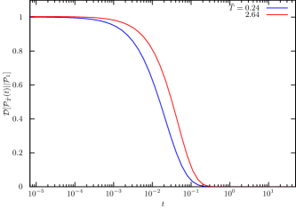
Figure S4: $\mathcal{D}[\mathcal{P}_{\tilde{T}^{\pm}}(t)||\mathcal{P}_{1}]$ as a function of time for a pair of equidistant quenches with $\tilde{T}^{+}=2.64$ and $\tilde{T}^{-}=0.24$, which illustrates the asymmetry in the thermal relaxation holds for any Gaussian Network (according to our proof).

II Tilted Single File

We consider a system of $N$ hard-core point-particles (the extension to a finite diameter is straightforward [2, 3]) diffusing in a box of unit length with a diffusion coefficient $D$, which we set equal to 1 and express energies in units of $k_{\mathrm{B}}T_{\mathrm{eq}}$ without any loss of generality. The particles with positions $\mathbf{x}=\{x_{i}\}$ feel the presence of a linear potential $U(\{x_{i}\})=\sum_{i=1}^{N}gx_{i}$. The Green’s function of the system obeys the many-body Fokker-Planck equation

$$(\partial_{t}-\hat{\mathcal{L}}_{\tilde{T}})G_{\tilde{T}}(\mathbf{x},t|\mathbf{x}_{0})\equiv\left(\partial_{t}-\sum_{i=1}^{N}(\partial_{x_{i}}^{2}+g\tilde{T}^{-1}\partial_{x_{i}})\right)G_{\tilde{T}}(\mathbf{x},t|\mathbf{x}_{0})=\delta(\mathbf{x}-\mathbf{x}_{0})$$ (S28)

The confining walls are assumed to be perfectly reflecting, i.e $J(x_{i})|_{x_{i}=0}=J(x_{i})|_{x_{i}=1}=-D(g/\tilde{T}-\partial_{x_{i}})G_{\tilde{T}}(\mathbf{x},t|\mathbf{x}_{0})=0,\forall i$. Moreover, particles are not allowed to cross, which introduces the following set of internal boundary conditions

$$\left(\partial_{x_{i+1}}-\partial_{x_{i}}\right)G_{\tilde{T}}(\mathbf{x},t|\mathbf{x}_{0})|_{x_{i+1}-x_{i}=0}=0,\forall i.$$ (S29)

Eq. (S28) with reflecting external boundary conditions $J(x_{i})|_{x_{i}=0}=J(x_{i})|_{x_{i}=1}=0,\forall i$ and internal boundary conditions in Eq. (S29) is solved exactly using the coordinate Bethe ansatz (we do not repeat the results here as they can be found in [4]). It is convenient to introduce the particle-ordering operator

$$\hat{\mathcal{O}}_{\mathbf{x}}\equiv\prod_{i=2}^{N}\theta(x_{i}-x_{i-1}),$$ (S30)

where $\theta(x)$ is the Heaviside step-function. Let $\zeta_{\tilde{T}}(x_{i},t|x_{0i})$ be the Green’s function of the corresponding single-particle problem and $P^{\mathrm{eq}}_{\tilde{T}}(x_{i})=\lim_{t\to\infty}\zeta_{\tilde{T}}(x_{i},t|x_{0i})$ the density of the equilibrium measure at temperature $\tilde{T}$, then the Green’s function can be written directly as

$$G_{1}(\mathbf{x},t|\mathbf{x}_{0})=N!\hat{O}_{\mathbf{x}}\prod_{i=1}^{N}\zeta_{1}(x_{i},t|x_{0i})\to P_{\tilde{T}}(\mathbf{x},t)=N!\hat{O}_{\mathbf{x}}\prod_{i=1}^{N}\int_{0}^{1}dx_{i0}\zeta_{1}(x_{i},t|x_{i0})P^{\mathrm{eq}}_{\tilde{T}}(x_{i0}),$$ (S31)

where the normalization factor $N!$ assures a correct re-weighing of non-crossing trajectories [4]. We expand the Green’s function for a single particle at $\tilde{T}=1$ in a bi-orthonormal eigenbasis, $\zeta(x,t|x_{0})=\sum_{k}\phi_{k}^{R}(x)\phi_{k}^{L}(x_{0})\mathrm{e}^{-\lambda_{k}t}$, where $\lambda_{0}=0$, $\lambda_{k}=\pi^{2}k^{2}+g^{2}/4$ and

$$\phi^{L}_{k}(x)=\frac{\mathrm{e}^{gx/2}}{\sqrt{2\lambda_{k}}}\left(g\sin(k\pi x)-2k\pi\cos(k\pi x)\right),k>0$$ (S32)

and $\phi^{R}_{k}(x)=\mathrm{e}^{-gx}\phi^{L}_{k}(x)$, whereas for $k=0$ we have $\phi^{L}_{0}(x)=1$, $\phi^{R}_{0}(x)=P_{1}^{\mathrm{eq}}(x)$.

A key simplification in the calculation of order-preserving integrals as well as all projected, tagged-particle observables (incl. functionals; see e.g. [4]) is the so-called ’extended phase space integration’ introduced by Lizana and Ambjörnsson [2, 3], according to which for any $1\leq M\leq N$ and some function $f(\mathbf{x})$ that is symmetric with respect to permutation of coordinates $x_{i}$

$$\hat{O}_{\mathbf{x}}\prod_{i=1}^{N}\int_{0}^{1}dx_{i0}f(\mathbf{x})\delta(z-x_{M})=\prod_{i=1}^{M-1}\int_{0}^{z}dx_{i0}\prod_{j=M+1}^{N}\int_{z}^{1}dx_{j0}\frac{f(x_{M}=z,\{x_{i\neq M}\})}{(M-1)!(N-M)!}.$$ (S33)

With the aid of Eq. (S33) it is possible to calculate the Kullback-Leibler divergence as

$$\mathcal{D}[P_{\tilde{T}}||P_{1}]=\int d\mathbf{x}P_{\tilde{T}}(\mathbf{x},t)\ln(P_{\tilde{T}}(\mathbf{x},t)/P_{1}(\mathbf{x}))\equiv\left[\int_{0}^{1}dxP^{1}_{\tilde{T}}(x,t)\ln(P^{1}_{\tilde{T}}(x,t)/P^{1}_{1}(x))\right]^{N},$$ (S34)

where $P^{1}_{\tilde{T}}(x,t)=\int_{0}^{1}dx_{0}\zeta_{1}(x,t|x_{0})P^{\mathrm{eq}}_{\tilde{T}}(x_{0})$, and the second equality is a result of applying Eq. (S33). The result in Eq. (S34) for a single file of 10 particles is depicted in Fig. (3a) in the Letter. For the sake of completeness, we also present the exact explicit result for $\langle U(t)\rangle_{\tilde{T}}\equiv gN\langle x(t)\rangle_{\tilde{T}}$, which reads

$$\langle U(t)\rangle_{\tilde{T}}=gN\left(\frac{1-\mathrm{e}^{g}+g}{g(1-\mathrm{e}^{g})}+8\sum_{k=1}^{\infty}\left(\frac{gk\pi}{\lambda_{k}}\right)^{2}\frac{(\tilde{T}-1)(\mathrm{e}^{g/2}-(-1)^{k})(\mathrm{e}^{g/\tilde{T}}-(-1)^{k}\mathrm{e}^{g/2})}{(\mathrm{e}^{g/\tilde{T}}-1)[(\tilde{T}-2)^{2}g^{2}+(2\pi k\tilde{T})^{2}]}\mathrm{e}^{-\lambda_{k}t}\right).$$ (S35)

The results for the non-Markovian tagged-particle dynamics can be derived analogously. The probability density function for tagging the $M$th particle is defined as

$$\mathcal{P}_{\tilde{T}}(z,t)=\hat{\Pi}_{\mathbf{x}}(z)P_{\tilde{T}}(\mathbf{x},t)\equiv\hat{O}_{\mathbf{x}}\prod_{i=1}^{N}\int_{0}^{1}dx_{i0}\delta(z-x_{\mathcal{T}})P_{\tilde{T}}(\mathbf{x},t)$$ (S36)

and since $P_{\tilde{T}}(\mathbf{x},t)$ is symmetric to permutation of particle indices Eq. (S33) can be applied. The exact result has the form of a spectral expansion and reads

$$\mathcal{P}_{\tilde{T}}(z,t)=\sum_{\mathbf{k}}V_{0\mathbf{k}}(z)\mathcal{V}_{\mathbf{k}0}^{\tilde{T}}\mathrm{e}^{-\lambda_{\mathbf{k}}t},$$ (S37)

where $\mathbf{k}=\{k_{i}\}$ is a $N$-tuple of non-negative integers and $\lambda_{\mathbf{k}}=\sum_{n=1}^{N}\lambda_{k_{n}}$ are Bethe eigenvalues of the operator $\hat{\mathcal{L}_{1}}=\sum_{i=1}^{N}(\partial_{x_{i}}^{2}+g\partial_{x_{i}})$ in a unit box under non-crossing conditions with $\lambda_{0}=0$ and $\lambda_{k_{i}}=\pi^{2}k_{i}^{2}+g^{2}/4,\forall k>0$. Let $N_{L}=\mathcal{T}-1$ and $N_{R}=N-\mathcal{T}$ be the total number of particles to the left and to the right of the tagged particle, respectively. Then $V_{0\mathbf{k}}(z)$ and $\mathcal{V}_{\mathbf{k}0}^{\tilde{T}}$ in Eq. (S37) are defined as

$$\!\!\!V_{0k}(z)=\frac{m_{\mathbf{k}}}{N_{L}!N_{R}!}\frac{2g\alpha}{\tilde{T}\Omega^{g}_{\tilde{T}}(0,1)}\sum_{\{k_{i}\}}T^{1}_{\mathcal{T}}(z)\prod_{i=1}^{N_{L}}L_{i}^{1}(z)\!\!\!\!\!\!\prod_{i=N_{L}+2}^{N}\!\!\!\!\!R_{i}^{1}(z)$$ (S38)

$$\!\!\!\mathcal{V}_{\mathbf{k}0}^{\tilde{T}}=\frac{N!}{N_{L}!N_{R}!}\frac{2g\alpha}{\tilde{T}\Omega^{g}_{\tilde{T}}(0,1)}\!\int_{0}^{1}\!\!dz\sum_{\{k_{i}\}}T^{\tilde{T}}_{\mathcal{T}}(z)\prod_{i=1}^{N_{L}}L_{i}^{\tilde{T}}(z)\!\!\!\!\!\!\prod_{i=N_{L}+2}^{N}\!\!\!\!\!R_{i}^{\tilde{T}}(z)$$ (S39)

where $\alpha=\tilde{T}/(2-\tilde{T})$, $\Omega^{g}_{\tilde{T}}(x,y)\equiv\mathrm{e}^{-gx/\tilde{T}}-\mathrm{e}^{-gy/\tilde{T}}$, and $m_{\mathbf{k}}=\prod_{i}n_{k_{i}}!$ is the multiplicity of the Bethe eigenstate corresponding to the $N$-tuple $\mathbf{k}$, and the number $n_{k_{i}}$ counts how many times the eigenindex $k_{i}$ appears in the Bethe eigenstate [4]. In Eq. (S39) we have introduced the auxiliary functions

$$T^{\tilde{T}}_{\mathcal{T}}(z)=P_{\tilde{T}}^{\mathrm{eq}}(z)\frac{\mathrm{e}^{gx/2}\left(g\sin(k_{\mathcal{T}}\pi z)-2k_{\mathcal{T}}\pi\cos(k_{\mathcal{T}}\pi z)\right)}{\sqrt{2\lambda_{k_{\mathcal{T}}}}},\forall k_{\mathcal{T}}>0$$ (S40)

and $T^{\tilde{T}}_{\mathcal{T}}(z)=P_{\tilde{T}}^{\mathrm{eq}}(z)$ for $k_{\mathcal{T}}>0$ where $P_{\tilde{T}}^{\mathrm{eq}}(z)$ is defined as

$$\mathcal{P}_{\tilde{T}}^{\mathrm{eq}}(z)=\frac{gN!}{N_{L}!N_{R}!}\frac{\Omega^{g}_{\tilde{T}}(0,z)^{N_{L}}\Omega^{g}_{\tilde{T}}(z,1)^{N_{R}}}{\tilde{T}\Omega^{g}_{\tilde{T}}(0,1)}\mathrm{e}^{-gz/\tilde{T}},$$ (S41)

as well as

$$L_{i}^{\tilde{T}}(z) = \begin{cases}\Omega_{\tilde{T}}^{g}(0,z)/\Omega_{\tilde{T}}^{g}(0,1),\quad k_{i}=0\\ \lambda_{\sqrt{\alpha}k_{i}}\Phi_{k_{i}}^{g,\alpha}(0,z)+k_{i}\pi g\Psi_{k_{i}}^{g,\alpha}(0,z)(\tilde{T}-1)/(2-\tilde{T}),\quad k_{i}>0\\ \end{cases}$$

$$R_{i}^{\tilde{T}}(z) = \begin{cases}\Omega_{\tilde{T}}^{g}(z,1)/\Omega_{\tilde{T}}^{g}(0,1),\quad k_{i}=0\\ \ \lambda_{\sqrt{\alpha}k}\Phi_{k_{i}}^{g,\alpha}(z,1)+k_{i}\pi g\Psi_{k_{i}}^{g,\alpha}(z,1)(\tilde{T}-1)/(2-\tilde{T}),\quad k_{i}>0,\ \end{cases}$$

Note that $\lambda_{xk}\equiv\pi^{2}(xk_{i})^{2}+g^{2}/4,\forall k>0$, and $\sum_{\{k_{i}\}}$ denotes the sum over all possible permutations of $\mathbf{k}$ and the functions $\Phi_{k}^{g,\alpha}(x,y)$ and $\Psi_{k}^{g,\alpha}(x,y)$ are defined as

$$\!\!\!\!\!\!\!\Phi_{k}^{g,\alpha}(x,y) = \frac{\mathrm{e}^{-gx/2\alpha}\sin(k\pi x)-\mathrm{e}^{-gy/2\alpha}\sin(k\pi y)}{\lambda_{\alpha k}\sqrt{2\lambda_{k}}}$$

$$\!\!\!\!\!\!\!\Psi_{k}^{g,\alpha}(x,y) = \frac{\mathrm{e}^{-gx/2\alpha}\cos(k\pi x)-\mathrm{e}^{-gy/2\alpha}\cos(k\pi y)}{\lambda_{\alpha k}\sqrt{2\lambda_{k}}}.$$ (S42)

Details of the calculations can be found in [4]. The evaluation of Kullback-Leibler divergence, $S_{\tilde{T}}(t),\mathcal{S}_{\tilde{T}}(t)$ as well as $\langle\mathcal{U}(t)\rangle_{\tilde{T}}$ cannot be carried out analytically and we therefore resort to efficient and accurate numerical quadratures. The results are presented in Fig. (3) in the Letter.

We performed extensive systematic calculations for different values of $g$ and $N$, various combinations of $\tilde{T}^{\pm}$ as well as for different choices for tagged particles. All these calculations gave the same qualitative picture – without any exceptions ’uphill’ relaxation was always faster. However, we are not able to prove rigorously that this is indeed always the case. Therefore, for the single file the universally faster uphill relaxation is only a conjecture.

III Non-existence of a unique relaxation asymmetry in multi-well potentials and generic conditions when the asymmetry is obeyed

In the letter we demonstrated that the relaxation in single-well potentials is faster uphill than downhill. We have proven that this is always the case near stable minima and for any reversible Ornstein-Uhlenbeck process. Based on additional physical arguments we hypothesized that the asymmetry is a general feature of diffusion in single-well potentials. However, as we remarked in the Letter, it is not difficult to construct counterexamples proving that the asymmetry is not a general phenomenon in all reversible ergodic diffusion processes.

To that end we condider Markovian diffusion in rugged, multi-well potentials parametrized by

$$U(x)=e(ax^{6}+bx^{4}+cx^{3}+dx^{2}),$$ (S43)

with some appropriately chosen constants $a,b,c,d$ and $e$. Let the dynamics evolve according to $\hat{L}_{\tilde{T}}=\partial^{2}_{x}-\tilde{T}^{-1}\partial_{x}F(x)$, where $F(x)=-6e(ax^{5}+4bx^{3}+3cx^{2}+2dx)$ in a finite domain $a\leq x\leq b$ with reflecting boundaries, and let the corresponding Green’s function be the solution of the following initial-boundary value problem

$$(\partial_{t}-\hat{L}_{\tilde{T}})G_{\tilde{T}}(x,t|x_{0})=\delta(x-x_{0}),\quad-(\partial_{x}-\tilde{T}^{-1}F(x))G_{\tilde{T}}(x,t|x_{0})|_{x=a}=-(\partial_{x}-\tilde{T}^{-1}F(x))G_{\tilde{T}}(x,t|x_{0})|_{x=b}=0.$$ (S44)

We solve the Fokker-Plank equation so defined via the Method of Lines. The results for three distinct parameter sets is shown in Fig. (S5).

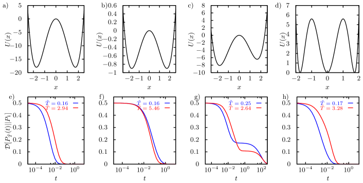
Figure S5: In panels a,b) and e,f) the potential is a quartic with parameter $a=0,b=1,c=0,d=-6,e=2$ in panels a and f and$a=0,b=1,c=0,d=-6,e=0.1$ in panels b and f. In the asymmetric potential in panels c and g with $a=0,b=1,c=0.2,d=-6,e=0.8$ and panels c and f with $a=1,b=-6,c=0,d=9,e=1.4$, respectively, the single-well asymmetry-pattern in fact becomes reversed. In a tripple-well with equally deep wells the asymmetry is again obeyed despite the middle well being wider.

We did not perform a systematic analysis of all the possible potentials. However, based on our observations it seems that the different uphill/downhill relaxation patterns depend on how different entropic contributions (i.e. intra-well entropy versus inter-well configuration entropy) change qualitatively with temperature for potentials with several minima.

If we focus on the asymmetric case (Fig. S5c) we find that uphill relaxation is initially always faster, which is a direct result of the physical mechanism at play that we present in the Letter. At longer time the asymmetry gets inverted by the slow inter-well partitioning of probability mass. It is now not diffcult to understand that by making the asymmetry smaller we will move the crossing point, where the corves intersect, closer to $\mathcal{D}[P_{\tilde{T}^{\pm}}(t)||P_{1}^{\mathrm{eq}}]=0$, such that for a sufficiently small asymmetry – which in the letter we refer to near degeneracy – uphill relaxation will eventually be faster for all times, for which $\mathcal{D}[P_{\tilde{T}^{\pm}}(t)||P_{1}^{\mathrm{eq}}]$ differs from zero by an amount that is not neglgible/detectable. For a formal discussion of this situation see below.

It is interesting and important to note that the asymmetry is also obeyed if the barrier is moderately high, i.e. such that a small but non-neglible probability mass is located at the barrier (see Fig. S6). However, the quench must then not be too strong. That is, an ’infinitely’ high barrier effecting a strict time-scale separation betwenn intra-well and inter-well relaxation is not a neccessarry condition for the asymmetry to occur. To demonstrate this we inspect overdamped relaxation according to Eq. (S44) in the following double well potential $U(x)=\Delta(x^{2}-1)^{2}$, where we choose (in units of $k_{\rm B}T_{\rm eq}$) $\Delta=3$ and $F(x)=-U(x)^{\prime}$.

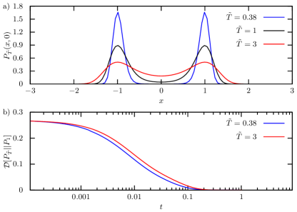
Figure S6: a) Density of invariant measure at $\tilde{T}=1$ (i.e. equilibrium probability density), and the equidistant post-quench probability densities at $\tilde{T}^{+}=3$ and $\tilde{T}^{-}=0.38$; b) Corresponding time evolution of the Kullback-Leibler divergence depicting that the asymmetry is obeyed.

In order to check that the observed effect in multi-well potentials is not an artifact of one-dimensional systems now also inspect 2-dimensional multi-well potentials. To that end we consider 4-well potentials parametrized by

$$U(x,y)=\Delta_{x}(x^{2}-x_{0}^{2})^{2}+\Delta_{y}(y^{2}-y_{0}^{2}),$$ (S45)

where energy is measured in units of $k_{\rm B}T_{\rm eq}$. We solve the problem by the Alternating Direction Implicit method (ADI) developed in [5] with 4-step operator splitting. We first focus on the limit of high barriers and quenches leaving the inter-well partitioning of probability mass unaffected (see Fig. S7). According to the proposed principle and prediction the symmetry is obeyes and uphill relaxation is always faster.

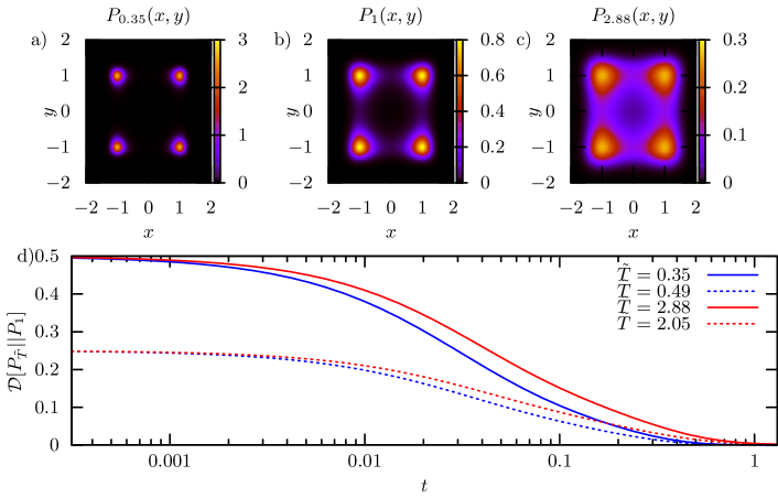
Figure S7: Density of invariant measure at $\tilde{T}=1$ (b) (i.e. equilibrium probability density), and the equidistant post-quench probability densities at (c) $\tilde{T}^{+}=2.88$ and (a) $\tilde{T}^{-}=0.35$ for the 4-well potential in Eq. (S45) with parameters $\Delta_{x}=\Delta_{y}=3$ and $x_{0}=y_{0}=1$.; d) Corresponding time evolution of the Kullback-Leibler divergence depicting that the asymmetry is obeyed for two pairs of equidistant temperatures.

In Fig. S8 now inspect the case of a moderately high barriers (where the probability density on top of the barriers does not vanishes). As expected the asymmetry is obeyed only for sufficiently small quenches, whereas it becomes violated for stronger quenches (compare full and dashed lines). The reason for the violation is the fact that the inter-well redistribution becomes the dominant step for strong quenches.

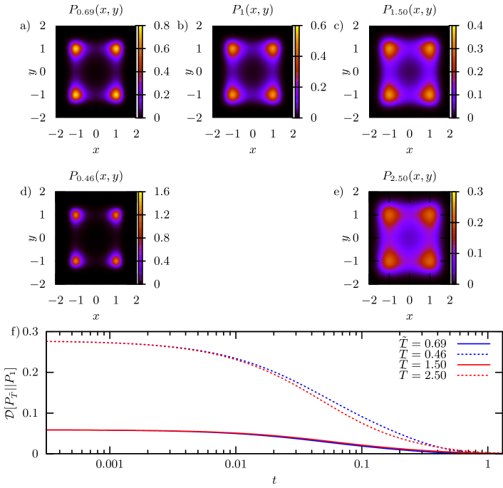
Figure S8: Density of invariant measure at (a) $\tilde{T}^{-}=0.69$ (b) at $\tilde{T}=1$, and at (c) $\tilde{T}^{+}=1.5$, (d) $\tilde{T}^{-}=0.46$ and (e) $\tilde{T}^{+}=2.5$ corresponding to the 4-well potential in Eq. (S45) with parameters $\Delta_{x}=\Delta_{y}=2$ and $x_{0}^{2}=y_{0}^{2}=1$.; b) Corresponding time evolution of the Kullback-Leibler divergence depicting that the asymmetry is obeyed for small quenches (a and c) and violated for strong quenches (d and e).

It seems that the asymmetry observed in single-well potentials persists in nearly degenerate potentials and ceases to exists as soon as the potential becomes sufficiently asymmetric with sufficiently deep wells, where entropy attains an additional inter-well configurational component, such that during relaxation the probability mass becomes re-distributed between the wells in an asymmetric manner.

III.1 The asymmetry is obeyed in degenerate potentials in the presence of a time-scale separation

We now provide also formal arguments confirming that the symmetry must be obeyed in degenerate potentials in the presence of a time-scale separation. We follow the work of Moro [6]. Since we are dealing with systems obeying detailed balance the generator of the relaxation dynamics $\hat{\mathcal{L}}$ is always diagonalizable, i.e.

$$\hat{\mathcal{L}}_{T}=\sum_{k\geq 0}-\lambda_{k}\psi_{k}^{R}(\mathbf{x})\psi_{k}^{L}(\mathbf{x}_{0})$$ (S46)

where $\psi_{k}^{R}(\mathbf{x})$ and $\psi_{k}^{L}(\mathbf{x})$ are the orthonormal right and left eigenfunctions, respectively, (i.e. $\int\psi_{k}^{L}(\mathbf{x})\psi_{l}^{R}(\mathbf{x})d\mathbf{x}=\delta_{kl}$) and $-\lambda_{k}$ are real eigenvalues ($\lambda_{0}=0$ as we have assumed that the potential is confining and the dynamics is ergodic). The eigenfunctions constitute a complete bi-orthonormal basis, $\sum_{k}\psi_{k}^{L}(\mathbf{x})\psi_{k}^{R}(\mathbf{x}^{\prime})=\delta(\mathbf{x}-\mathbf{x}^{\prime})$. As a result of detailed balance we have $\psi_{k}^{R}(\mathbf{x})=\mathrm{e}^{-U(\mathbf{x})/k_{\rm B}T}\psi_{k}^{L}(\mathbf{x})$ and $\psi_{0}^{R}(\mathbf{x})=P_{T}^{\mathrm{eq}}\equiv\mathrm{e}^{-U(\mathbf{x})/k_{\rm B}T}/\int\mathrm{e}^{-U(\mathbf{x})/k_{\rm B}T}d\mathbf{x}$ and $\psi_{0}^{L}(\mathbf{x})=1$. Let $\hat{\mathcal{L}}_{T}^{\dagger}$ be the adjoint (or ’backward’) generator, then we have the pair of eigenproblems $\hat{\mathcal{L}}_{T}\psi_{k}^{R}(\mathbf{x})=-\lambda_{k}\psi_{k}^{R}(\mathbf{x})$ and $\hat{\mathcal{L}}^{\dagger}_{T}\psi_{k}^{L}(\mathbf{x})=-\lambda_{k}\psi_{k}^{L}(\mathbf{x})$.

The Green’s function of the relaxation problem, $(\partial_{t}-\hat{\mathcal{L}}_{T})G_{T}(\mathbf{x},t|\mathbf{x}_{0})=0$ with $G_{T}(\mathbf{x},0|\mathbf{x}_{0})=\delta(\mathbf{x}-\mathbf{x}_{0})$, decomposes to

$$G_{T}(\mathbf{x},t|\mathbf{x}_{0})=\sum_{k\geq 0}\psi_{k}^{R}(\mathbf{x})\psi_{k}^{L}(\mathbf{x}_{0})\mathrm{e}^{-\lambda_{k}t}\to\quad P_{\tilde{T}}(\mathbf{x},t)=\int G_{1}(\mathbf{x},t|\mathbf{x}_{0})P_{\tilde{T}}^{\mathrm{eq}}(\mathbf{x}_{0})d\mathbf{x}_{0}.$$ (S47)

In presence of a time-scale separation (as a result of the existence of one or more high energy barriers) the eigenvalue spectrum of $\hat{\mathcal{L}}$ has a gap, i.e. $\exists k_{\rm min}$ such that $\lambda_{k_{\rm min}+l}\gg k_{\rm min}\forall l\geq 1$.

Assume now a set of $M$ well-defined deep minima at $\hat{\mathbf{x}}_{i},i=1,\ldots,M$. This implies $k_{\rm min}=M-1$. Let us define localizing functions $g_{i}(\mathbf{x}),i\in[1,M]$ such that

$$c_{i}^{\mathrm{eq}}\equiv\int g_{i}(\mathbf{x})P_{1}^{\mathrm{eq}}(\mathbf{x})d\mathbf{x}\quad\to\quad\int g_{i}(\mathbf{x})\psi_{k}^{R}(\mathbf{x})=0,\forall k\geq M,$$ (S48)

$c_{i}^{\mathrm{eq}}$ are the equilibrium site populations. The localizing functions therefore by definition separate the intra-well relaxation from the inter-well ’hopping’ of probability mass. In turn this implies that $g_{i}(\mathbf{x})$ belong to the subspace $\{\psi_{k}^{L}(\mathbf{x})\},k<M$, i.e.

$$g_{i}(\mathbf{x})=\sum_{k=0}^{M-1}B_{ik}\psi_{k}^{L}(\mathbf{x}),\forall i\in[1,M]$$ (S49)

and are thus by construction linearly independent but are so far only defined up to the expansion matrix $\mathbf{B}$. We determine $\mathbf{B}$ by imposing that the localizing functions should be localized near only one minimum $\hat{\mathbf{x}}_{i}$ and vanish at all remaining minima, i.e. $g_{i}(\hat{\mathbf{x}}_{j})\simeq\delta_{i,j}$. Let the inverse of $\mathbf{B}$ be $\mathbf{B}^{-1}$, $\mathbf{B}^{-1}\mathbf{B}=\mathbbm{1}$. We finally fix $g_{i}(\mathbf{x})$ by imposing the following resolution of identity $\sum_{I=1}^{M}g_{i}(\mathbf{x})=1$, which allows us to write

$$\psi_{i}^{L}(\mathbf{x})=\sum_{k=1}^{M}B^{-1}_{ik}g_{k}(\mathbf{x}),\forall i\in[0,M-1],$$ (S50)

We now define the time-dependent population of the localizing sites (i.e. basins)

$$c_{i}(t)\equiv\int g_{i}(\mathbf{x})G(\mathbf{x},t|\mathbf{x}_{0})d\mathbf{x}.$$ (S51)

The fact that $g_{j}(\mathbf{x})$ decompose unity implies that the total site population is conserved in time, i.e.

$$\sum_{i=1}^{M}c_{i}(t)\equiv\sum_{i=1}^{M}\int g_{i}(\mathbf{x})G(\mathbf{x},t|\mathbf{x}_{0})d\mathbf{x}=\int\sum_{i=1}^{M}g_{i}(\mathbf{x})G(\mathbf{x},t|\mathbf{x}_{0})d\mathbf{x}=1,$$ (S52)

where we have used the fact that the integral and sum commute by Fubini’s theorem (note that we can write the sum as an integral with respect to a counting measure). The localizing functions are linearly independent but not orthonormal. For this purpose we define the $M\times M$ superposition matrix $\mathbf{S}$ with elements $S_{ij}\equiv\int g_{i}(\mathbf{x})P_{1}^{\mathrm{eq}}(\mathbf{x})g_{j}(\mathbf{x})d\mathbf{x}$ such that we can re-write the equilibrium site population as

$$c_{i}^{\mathrm{eq}}=\int g_{i}(\mathbf{x})P_{1}^{\mathrm{eq}}(\mathbf{x})\sum_{j=1}^{M}g_{j}(\mathbf{x})d\mathbf{x}=\sum_{j=1}^{M}S_{ij}.$$ (S53)

We now define a projection operator projecting onto the space of localizing functions

$$\hat{\mathrm{P}}q(\mathbf{x})\equiv\sum_{i=1}^{M}q_{i}g_{i}(\mathbf{x}),\quad q_{i}\equiv\sum_{k=1}^{M}S^{-1}_{i,k}\int g_{i}(\mathbf{x})P_{1}^{\mathrm{eq}}(\mathbf{x})q(\mathbf{x})d\mathbf{x}.$$ (S54)

The time evolution of site populations then follows

$$\frac{dc_{j}(t)}{dt} = \int g_{j}(\mathbf{x})\partial_{t}G_{\tilde{T}}(\mathbf{x},t|\mathbf{x}_{0})d\mathbf{x}=\int g_{j}(\mathbf{x})\hat{\mathcal{L}}_{1}G_{\tilde{T}}(\mathbf{x},t|\mathbf{x}_{0})d\mathbf{x}=\int G_{\tilde{T}}(\mathbf{x},t|\mathbf{x}_{0})\hat{\mathcal{L}}_{1}^{\dagger}g_{j}(\mathbf{x})d\mathbf{x}$$ (S55)

$$\equiv \int G_{\tilde{T}}(\mathbf{x},t|\mathbf{x}_{0})\hat{\mathrm{P}}\hat{\mathcal{L}}_{1}^{\dagger}g_{j}(\mathbf{x})d\mathbf{x}=\sum_{k,i}c_{k}(t)S^{-1}_{k,i}\int g_{i}(\mathbf{y})\hat{\mathcal{L}}_{1}^{\dagger}P_{1}^{\mathrm{eq}}(\mathbf{y})g_{j}(\mathbf{y})d\mathbf{y}\equiv\sum_{k,i}c_{k}(t)S^{-1}_{k,i}\Gamma_{ij},$$ (S56)

where in the second line we used the fact that $\hat{\mathcal{L}}_{1}^{\dagger}g_{j}(\mathbf{x})$ already lies in the subspace of localizing functions (because $\hat{\mathcal{L}}^{\dagger}_{T}\psi_{k}^{L}(\mathbf{x})=-\lambda_{k}\psi_{k}^{L}(\mathbf{x})$ and Eq. (S49)) and the projection operator projects back onto said subspace. By defining $\mathbf{c}(t)=(c_{i}(t),\ldots,c_{M}(t))^{T}$ we recognize from Eq. (S56) that the site populations obey the Markovian master equation

$$\frac{d}{dt}\mathbf{c}(t)=\mathbf{M}\mathbf{c}(t),\quad M_{jk}\equiv\sum_{i}S^{-1}_{k,i}\Gamma_{ij},$$ (S57)

where it can be shown that the transition rates entering $\mathbf{M}$ obey detailed balance [6]. It is obvious that $\mathbf{M}\mathbf{c}^{eq}=0$ and therefore an equilibrated site-population does not lead to any inter-well dynamics. The evolution upon a temperature quench from $\tilde{T}$ follows from the evolution of the Green’s function, i.e. $P_{\tilde{T}}(\mathbf{x},t)=\int G_{1}(\mathbf{x},t|\mathbf{x}_{0})P_{\tilde{T}}^{\mathrm{eq}}(\mathbf{x}_{0})d\mathbf{x}_{0}$. Therefore, any quench that will leave the site populations given the potential $U(\mathbf{x})$ and Fokker-Planck operator $\hat{\mathcal{L}}_{1}$ ($\hat{\mathcal{L}}_{1}^{\dagger}$ respectively) almost unaffected, i.e.

$$\mathbf{M}\mathbf{c}(0)\simeq 0,\quad{\rm where}\quad c_{i}(0)=\int g_{i}(\mathbf{x})P_{\tilde{T}}(\mathbf{x},t=0|\mathbf{x}_{0})d\mathbf{x}\equiv\int g_{i}(\mathbf{x}_{0})P_{\tilde{T}}^{\mathrm{eq}}(\mathbf{x}_{0})d\mathbf{x}_{0},$$ (S58)

will lead to a faster uphill relaxation as a direct consequence of the fact that the intra-well (i.e. in each individual well) relaxation is faster uphill. The above arguments can be arranged in a form that is fully rigorous, but since the argumentation is essentially straightforward, we do not find it necessary to do so.

III.2 Small local modulations do not spoil the asymmetry

As stated in the Letter, small local modulations of the potential ($\ll k_{\rm B}T_{\mathrm{eq}}$) do not affect the asymmetry as longs as the uphill quench is sufficiently small to assure that the modulation is $\lesssim k_{\rm B}T^{-}$ . Then the system relaxes similarly as in a perfectly smooth single well. To demonstrate that this is indeed the case we inspect the relaxation from equidistant quenches in the potential in Eq. (S45) with $\Delta_{x}=\Delta_{y}=2$ and $x_{0}^{2}=y^{2}=0.4$ depicted in Fig. S9. If, however, we make the quench too severe, such that the local modulations of the potential effectively reach $|\Delta U(\mathbf{x})|\gtrsim k_{\rm B}T^{-}$ the asymmetry would become violated and the curves will eventually cross, rendering downhill relaxation faster.

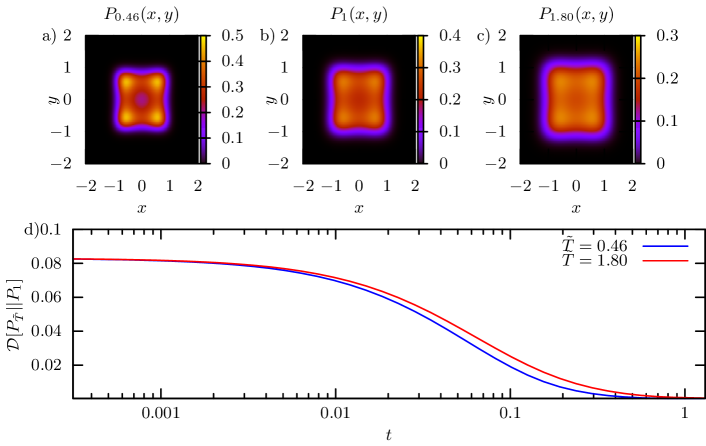
Figure S9: a) Density of invariant measure at $\tilde{T}=1$ (i.e. equilibrium probability density), and the equidistant post-quench probability densities at $\tilde{T}^{+}=1.8$ and $\tilde{T}^{-}=0.46$ for the 4-well potential in Eq. (S45) with parameters $\Delta_{x}=\Delta_{y}=2$ and $x_{0}^{2}=y_{0}^{2}=0.4$.; b) Corresponding time evolution of the Kullback-Leibler divergence depicting that the asymmetry is obeyed.

A a final example we focus on an asymmetric quadruple-well with a pair of high barriers and a pair of low barriers (the latter creating a small local modulation of the potential). In particular, we consider the relaxation in the potential given in Eq. (S45) with parameters $\Delta_{x}=3,\Delta_{y}=2$ and $x_{0}=0.5,y_{0}=1$ and inspect in Fig. S10 the following pairs of thermodynamically equidistant temperatures, $\tilde{T}^{-}=0.8,\tilde{T}^{+}=1.25$ and $\tilde{T}^{-}=0.5,\tilde{T}^{+}=2.$.

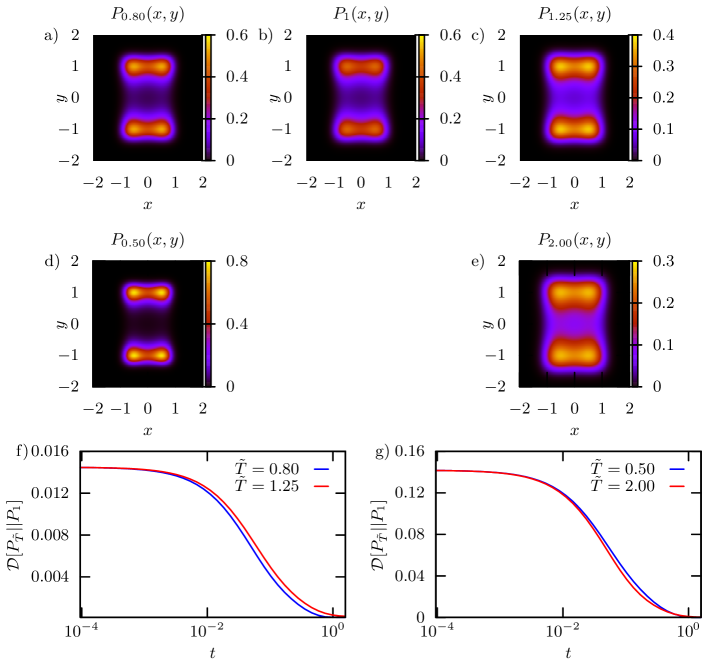
Figure S10: b) Density of invariant measure at $\tilde{T}=1$ (i.e. equilibrium probability density), and two pairs of equidistant post-quench probability densities at $\tilde{T}^{+}=1.25$ (c) and $2$ (e) and corresponding equidistant $\tilde{T}^{-}=0.8$ (a) and $0.5$ (d), respectively, for the 4-well potential in Eq. (S45) with parameters $\Delta_{x}=3,\Delta_{y}=2$ and $x_{0}=0.5,y_{0}=1$.; f-g) Corresponding time evolution of the Kullback-Leibler divergence depicting that the asymmetry is obeyed for small enough quenches but becomes violated (in the form of an Mpemba-like effect) for stronger quenches.

As anticipated, the uphill relaxation is faster for sufficiently small quenches (see Fig. S10f) and becomes violated for stronger quenches (see Fig. S10g), where the Kullback-Leibler divergences also display an Mpemba-like effect (see also next section).

IV Generalized Mpemba effect for non-Markovian dynamics

A phenomenon closely linked to relaxation from a quench is the so-called Mpemba effect [7, 8, 9], according to which a liquid upon cooling can freeze faster if its initial temperature is higher. Meanwhile the phenomenon has been extended to cover relaxation processes in different systems: magneto-resistors [10], carbon-nanotubes [11], polymers crystallization [12], clathrate hydrates [13], granular systems [14] and spin glasses [15]. Recently theoretical generalizations of it for Markovian observables have been published [16, 17, 18]. Not long ago the phenomenon was also adressed in more detail in the context of Markovian stochastic dynamics [16, 18].

Here we further extend the concept of the Mpemba effect to projected, non-Markovian observables. As before we focus on the distance of two different generic configurations displaced from equilibrium at $t=0$, such that one is displaced further away than the other, whereas the time-evolution of the entire system is governed by the same Fokker-Planck operator. In this setting, there are cases, where the more distant initial configuration reaches equilibrium faster that the closer one. One can observe this effect in the two systems analyzed in the Letter (see Fig. S11).

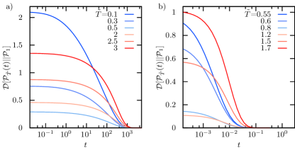
Figure S11: In the left panel we show time dependence of the Kullback-Leibler divergence for a Gaussian Chain of 100 beads, while the right panel depicts a Single File of 10 particles ($g=5$). In both cases we focus on non-Markovian observables, the end-to-end distance for the Gaussian chain and on the 7th particle of the single file, respectively. For some pairs of initial temperatures we notice the generalized Mpemba effect: systems that start further away from the equilibrium approach the equilibrium configuration faster.

It is worth to stress that the presence of the generalized Mpemba effect not only depends on the system and the initial condition (like in the Markovian case) but also on the particular type of projection In Fig. S12 we demonstrate, on hand of the same system (a tilted single file of 5 particles) from the same pair of pre-quench temperatures, that we can switch the generalized Mpemba effect on and off by simply changing the particle we are tagging.

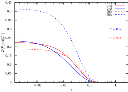
Figure S12: Kullback-Leibler divergences for a single file of 5 particles with $g=1$. If we tag the 2nd particle (solid lines) or the 5th (dashed lines) for the same pair of pre-quench temperatures one projection displays the generalized Mpemba effect while the other one does not.

References

Supplementary Material for: