Model of a gap formed by a planet with fast inward migration

Abstract

A planet is formed within a protoplanetary disk. Recent observations have revealed substructures such as gaps and rings, which may indicate forming planets within the disk. Due to disk–planet interaction, the planet migrates within the disk, which can affect a shape of the planet-induced gap. In this paper, we investigate effects of fast inward migration of the planet on the gap shape, by carrying out hydrodynamic simulations. We found that when the migration timescale is shorter than the timescale of the gap-opening, the orbital radius is shifted inward as compared to the radial location of the gap. We also found a scaling relation between the radial shift of the locations of the planet and the gap as a function of the ratio of the timescale of the migration and gap-opening. Our scaling relation also enables us to constrain the gas surface density and the viscosity when the gap and the planet are observed. Moreover, we also found the scaling relation between the location of the secondary gap and the aspect ratio. By combining the radial shift and the secondary gap, we may constrain the physical condition of the planet formation and how the planet evolves in the protoplanetary disk, from the observational morphology.

1 Introduction

In a protoplanetary disk, a planet is formed and its orbital radius of the planet varies by gravitational interaction to the surrounding gas (e.g., Lin & Papaloizou, 1979; Goldreich & Tremaine, 1980), and its mass increases by the gas accretion onto the planet (e.g., Bryden et al., 1999; Kley, 1999; D’Angelo et al., 2003; Tanigawa & Watanabe, 2002; Machida et al., 2010). Moreover, when the mass of the planet is massive enough, the planet opens a density gap along with its orbit and it migrates with the gap (e.g., Lin & Papaloizou, 1986; Edgar, 2007; Crida & Morbidelli, 2007; Dürmann & Kley, 2015, 2017; Kanagawa et al., 2018b; Kanagawa, 2019). Outside of the gap, moreover, relatively large dust grains can be piled-up and a ring structure can be formed (e.g., Paardekooper & Mellema, 2004; Muto & Inutsuka, 2009; Zhu et al., 2012; Dong et al., 2015; Weber et al., 2018; Kanagawa et al., 2018a). Such gap/ring structures in protoplanetary disks can be considered as a signal of the planet formation.

Recent observations have revealed a large diversity of exoplanets including a close-in giant planet (Hot Jupiter) and Super-Earths (e.g., Winn & Fabrycky, 2015), and giant planets orbiting at large radii (e.g., Hashimoto et al., 2011). Although the origin of the diversity is still not understood, it could be related to how the planets form and evolve within protoplanetary disks. Thanks to e.g., the Atacama Large Millimeter/submillimeter Array (ALMA) and Subaru telescope, substructures such as rings, gaps, and spirals have been observed at protoplanetary disks (e.g., Fukagawa et al., 2013; ALMA Partnership et al., 2015; Akiyama et al., 2015; Momose et al., 2015; van der Plas et al., 2017; Fedele et al., 2017; Dong et al., 2018b; Long et al., 2018; van der Marel et al., 2019). From the depth and width of the observed gap, one can estimate the mass of the unseen planet embedded in the disk (e.g., Kanagawa et al., 2015, 2016; Rosotti et al., 2016; Zhang et al., 2018), if the gap is formed by the planet. Moreover, recent observations have discovered point sources in the protoplanetary disks, PDS 70 (Keppler et al., 2018; Müller et al., 2018), TW Hya (Tsukagoshi et al., 2019), which are candidates of the forming planet. These observations enable us to know the presence of the planet in the present stage. To reveal when and where the planet is formed, however, we need to consider how the planet evolves within the protoplanetary disk. It is still an open question how the planet evolves within the protoplanetary disks, though it has been actively studied from a theoretical point of view (e.g., Mordasini et al., 2012; Ida et al., 2013; Bitsch et al., 2015b; Ida et al., 2018; Johansen et al., 2019; Tanaka et al., 2019).

Meru et al. (2019) and Nazari et al. (2019) have investigated observational signatures of the planetary migration by focusing on locations of gas pressure bumps and dust rings. Weber et al. (2019) have also investigated the effects of the migration on the location of the dust rings in the case of low viscosity. Meru et al. (2019) also pointed out that the location of the planet can be shifted from the center of the gap. In this paper, we further investigate effects of the planetary migration on the locations of the planet and gaps, which could be applied to the observation of the gas in near future. From the recent ALMA observations, in the relatively outer region ($>30$ AU), the width of some observed gaps is relatively narrow and thus the planet mass estimated from the gap shape can be not so massive, typically Neptune size to sub-Jupiter size (e.g., Dipierro et al., 2015; Kanagawa et al., 2015; Nomura et al., 2016; Tsukagoshi et al., 2016; Zhang et al., 2018) when the gas viscosity is low as implied by observations (e.g. Pinte et al., 2016; Flaherty et al., 2015; Teague et al., 2016). Hence, we focus on the observational signatures from the Neptune-sized planet in this paper. We describe our model in Section 2 and present our results in Section 3. In Section 4, we discuss feasibility of observations and how to constrain the evolution of the planet from the observational signatures. We summarize our results in Section 5.

2 Basic equations and our model description

2.1 Basic equations

We investigate effects of a migrating planet on the gap structure, by carrying out two-dimensional hydrodynamic simulations with a planet. In our simulations, we use a geometrically thin and non-self-gravitating disk. We choose a two-dimensional cylindrical coordinate system $(R,\phi)$, and its origin locates at the position of the central star. The velocity is denoted as $\vec{v}=(\rm{v}_{R},\rm{v}_{\phi})$, where $\rm{v}_{R}$ and $\rm{v}_{\phi}$ are the velocities in the radial and azimuthal directions. The angular velocity is denoted by $\Omega=\rm{v}_{\phi}/R$. We adopt a simple isothermal equation of state, in which the vertically integrated pressure $P$ is given by $c_{s}^{2}\Sigma$, where $c_{s}$ is the isothermal speed of sound.

The vertically integrated equation of continuity is

$$\frac{\partial\Sigma}{\partial t}+\nabla\cdot\left(\Sigma\vec{v}\right) =0.$$ (1)

The equations of motion are

$$\frac{\partial\vec{v}}{\partial t}+\vec{v}\cdot\nabla\vec{v} =-\frac{\nabla P}{\Sigma}-\nabla\Psi+\vec{f}_{\nu},$$ (2)

where $\vec{f}_{\nu}$ represents the viscous force per unit mass (c.f., Nelson et al., 2000). The gravitational potential $\Psi$ is given by the sum of the gravitational potentials of the star and the planet as

$$\Psi =-\frac{\rm{G}M_{\ast}}{R}+\Psi_{p}+\frac{\rm{G}M_{\rm p}}{R_{\rm p}^{2}}R\cos\left(\phi-\phi_{p}\right),$$ (3)

where $\rm{G}$ is the gravitational constant. The first term of Equation (3) is the potential of the star and the third term represents the indirect terms due to planet–star gravitational interaction. The second term is the gravitational potential of the planet, which is given by

$$\Psi_{p} =-\frac{\rm{G}M_{\rm p}}{\left[R^{2}+2RR_{\rm p}\cos\left(\phi-\phi_{p}\right)+R_{\rm p}^{2}+\epsilon^{2}\right]^{1/2}},$$ (4)

where $\epsilon$ is a softening parameter.

2.2 Our setup of hydrodynamic simulations

To numerically solve Equations (1) and (2), we use the two-dimensional numerical hydrodynamic code FARGO Masset (2000), which is an Eulerian polar grid code with a staggered mesh. The softening parameter $\epsilon$ in the gravitational potential of Equation (4) is set to be $0.6$ times the disk scale height at the location of the planet. Considering the existence of the circumplanetary disk, we exclude $60\%$ of the planets’ Hill radius when calculating the force exerted by the disk on the planet. For simplicity, we neglect the disk gas accretion onto the planet.

From the relation between the planet mass and the width (and depth) of the gap, we can estimate the mass of the planet within the observed gap (e.g., Kanagawa et al., 2015; Rosotti et al., 2016; Dong & Fung, 2017; Zhang et al., 2018). Recent observations have revealed relatively narrow gaps which can be carved by the planet around the Neptune-mass to sub-Jupiter mass, for instance, the gap at $\sim 70$ AU in the disk around HL Tau ($M_{\rm p}\simeq 0.3M_{J}$ with $\alpha=10^{-3}$, the same $\alpha$ is assumed for the following planet mass) (e.g., Kanagawa et al., 2016; Jin et al., 2016), the gap at $22$ AU in the disk of TW Hya ($M_{\rm p}\simeq 0.06M_{J}$) (Tsukagoshi et al., 2016), the gap at $97$ AU in the disk of RX J1615e ($M_{\rm p}=0.22M_{J}$) (Dong & Fung, 2017), and the gap at $69$ AU of Elias 27 disk ($M_{\rm p}\sim 0.1M_{J}$), the gap at $86$ AU in the disk of HD 163296 ($M_{\rm p}\simeq 0.3M_{J}$) (Zhang et al., 2018). Moreover, recent observation done by Tsukagoshi et al. (2019) has discovered the excess of the millimeter flux at $\sim 50$ AU. From the excess of the flux, the mass of the planet is estimated as the Neptune size. Hence, in this paper, we adopt the mass of the planet around Neptune-mass.

The recent observations give an upper limit on the $\alpha$-parameter on the viscosity for a few protoplanetary disks, namely, $\alpha\lesssim 10^{-3}$ in the disk of HD 163296 (Flaherty et al., 2015, 2017) and in the disk of TW Hya (Teague et al., 2016; Flaherty et al., 2018). Motivated by those observations, we adopt a relatively small value of $\alpha$.

The computational domain runs from $R=0.1R_{0}$ to $R=2.4R_{0}$, where we use a unit of the radius as an arbitrary value $R_{0}$ and a unit of the mass as $M_{\ast}$ (the mass of the central star). The domain is divided into 512 meshes in the radial direction (logarithmic equal spacing) and 1024 meshes in the azimuthal direction (equal spacing). The orbital radius of the planet is initially set to be $R=R_{0}$. The surface density is thus normalized by $M_{\ast}/R_{0}^{2}$, and we choose $M_{\ast}=1M_{\odot}$ as the fiducial value. Since focusing on the planet orbiting at larger radii, we assume $R_{0}=100$ AU in this paper. For convenience, we define $t_{0}$ as the Keplerian orbital time at $R=R_{0}$. We compute the migration of the planet during $t=1000\ t_{0}$ (which corresponds to 1 Myr when $R_{0}=100$ AU). We assume a uniform distribution of the disk aspect ratio, $h/R=0.05$. Since we adopt a structure in steady state of viscous accretion disk (c.f. Lynden-Bell & Pringle, 1974) as the initial condition, the unperturbed distribution of the surface density given by

$$\Sigma_{\rm un}(R)=\Sigma_{0}\left(\frac{R}{R_{0}}\right)^{-1/2}.$$ (5)

The initial angular velocity of the gas is given by $\Omega_{\rm K}\sqrt{1-2\eta}$, where $\eta=(1/2)(h/R)^{2}d\ln P/d\ln R$. The initial radial drift velocity of the gas is given by $v_{R}=-3\nu/(2R)$. The parameters we investigate in this paper are summarized in Table 1. Note that when $M_{\ast}=1M_{\odot}$ and $R_{0}=100$ AU, the surface density is $0.9\rm{g/cm}^{2}(\Sigma_{0}/10^{-3})$ at $R=100$ AU. For simplicity we do not consider growth of the mass of the planet, whereas the planetary orbit varies with time according to the disk-planet interaction.

Table 1: Parameters

$\alpha$	$\Sigma_{0}$	$M_{\rm p}/M_{\ast}$	$H_{0}$
$5\times 10^{-5}$	$[1,3,5,7,10]\times 10^{-4}$	$5\times 10^{-5}$	$0.05$
$1\times 10^{-4}$	$[1,3,5,7,10]\times 10^{-4}$	$5\times 10^{-5}$	$0.05$
$3\times 10^{-4}$	$[1,3,5,7,10]\times 10^{-4}$	$5\times 10^{-5}$	$0.05$
$5\times 10^{-4}$	$[1,5,10]\times 10^{-4}$	$5\times 10^{-5}$	$0.05$
$1\times 10^{-3}$	$[1,3,5,7,10]\times 10^{-4}$	$5\times 10^{-5}$	$0.05$
$1\times 10^{-4}$	$[1,3,5,7,10]\times 10^{-4}$	$1\times 10^{-4}$	$0.05$
$1\times 10^{-3}$	$[1,3,5,7,10]\times 10^{-4}$	$1\times 10^{-4}$	$0.05$
$5\times 10^{-5}$	$[1,5,10]\times 10^{-4}$	$5\times 10^{-5}$	$0.07$
$1\times 10^{-4}$	$[1,5,10]\times 10^{-4}$	$5\times 10^{-5}$	$0.07$
$1\times 10^{-4}$	$[1,5,10]\times 10^{-4}$	$1\times 10^{-4}$	$0.07$
$5\times 10^{-5}$	$[1,5,10]\times 10^{-4}$	$1\times 10^{-4}$	$0.1$

At the inner and outer boundaries, the velocity of the gas is set to be the initial value. The surface density of the gas is also set so that the mass flux is constant. We define wave-killing zones which are located from $R_{\rm out}-0.1R_{0}$ to $R_{\rm out}$ for the outer boundary and from $R_{\rm in}$ to $R_{\rm in}+0.1R_{0}$ for the inner boundary, where $R_{\rm out}$ and $R_{\rm in}$ are the radius of the outer and inner boundaries, respectively. To avoid an artificial wave reflection, we force all the physical quantities to be azimuthally constant within the wave-killing zones, by overwriting the quantities with their azimuthal average at every time step (c.f., de Val-Borro et al., 2006; Kanagawa et al., 2017b).

3 Results of hydrodynamic simulations

3.1 Radial shift between the locations of the planet and the gap

Here, we define the location of the gap as the location where the azimuthally averaged surface density normalized by the unperturbed surface density $\Sigma_{\rm un}$ is the minimum in the region of $R>R_{\rm p}$ . We denote this radius of the gap as $R_{\rm gap}$, and $R_{\rm p}$ denotes the orbital radius of the planet. In our simulations, the secondary gap is formed in the inner disk of the planet, as shown by e.g., Bae et al. (2017); Dong et al. (2017). For convenience, we define the location of the secondary gap $R_{\rm gap}^{\rm 2nd}$ as the position where $\Sigma/\Sigma_{\rm un}$ takes the first local minimum from $R_{\rm p}$ in the inner disk.

The depth of the secondary gap $\delta_{\rm gap}^{\rm 2nd}$ is defined by the ratio of the surface densities at $R=R_{\rm gap}^{\rm 2nd}$ and the position where $\Sigma/\Sigma_{\rm un}$ takes the first local maximum from $R_{\rm p}$ in the inner disk. In Figure 1, we illustrate the definitions of $R_{\rm gap}$, $R_{\rm gap}^{\rm 2nd}$ and $\delta_{\rm gap}^{\rm 2nd}$.

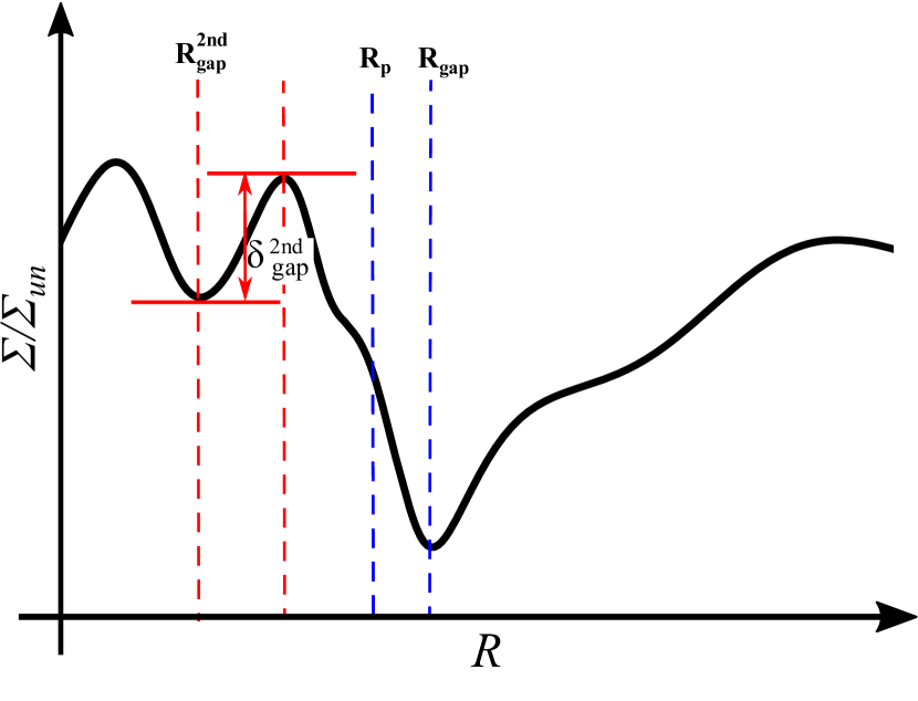
Figure 1: Schematic picture for the definition of the location of the (primary) gap $R_{\rm gap}$, the location of the secondary gap $R_{\rm gap}^{\rm 2nd}$, and the depth of the secondary gap $\delta_{\rm gap}^{\rm 2nd}$.

First we show the results in the case of $M_{\rm p}/M_{\ast}=5\times 10^{-5}$, $h/R=0.05$, and $\alpha=1\times 10^{-4}$, as the fiducial case.

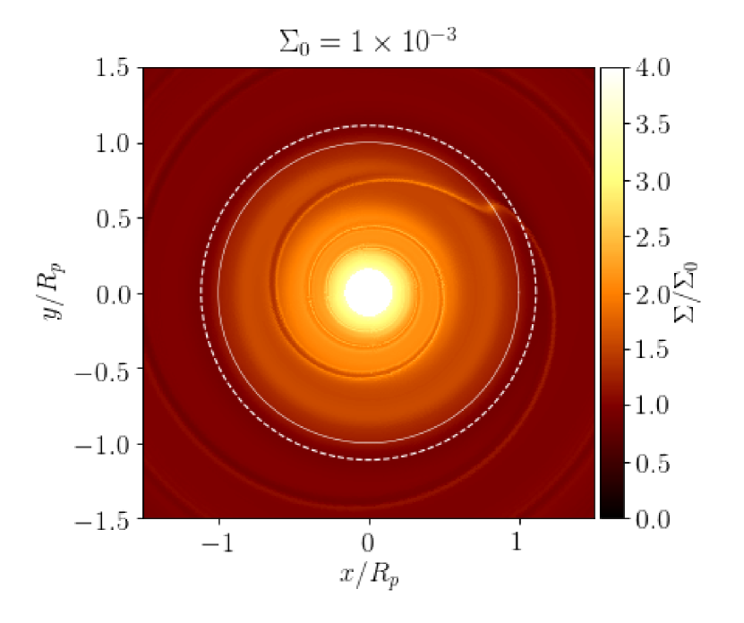
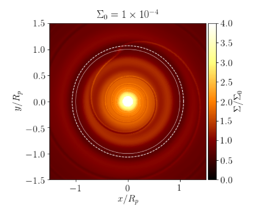
Figure 2: Two-dimensional distributions of the gas surface density in the cases of $\Sigma_{0}=1\times 10^{-3}$ (Left) and $\Sigma_{0}=10^{-4}$ (Right) at $t=1000\ t_{0}$. The mass of the planet is $M_{\rm p}/M_{\ast}=5\times 10^{-5}$, and $H_{0}=0.05$ and $\alpha=10^{-4}$, respectively. The white solid and dashed lines denote the orbital radius of the planet ($R=R_{\rm p}$)and the radial position of the gap (location with the minimum surface density within the gap, $R=R_{\rm gap}$). The vertical and horizontal axes are normalized by $R_{\rm p}$, and $R_{\rm p}=0.61R_{0}$ in the right panel and $R_{\rm p}=0.95R_{0}$ in the left panel, respectively (see also Figure 3).

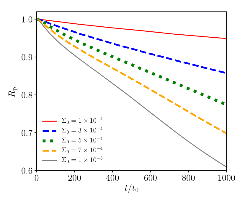
Figure 3: Time variations of the semi-major axis of the planet for various values of $\Sigma_{0}$. The planet mass, aspect ratio and the viscosity are the same as those of the case shown in Figure 2 ($M_{\rm p}/M_{\ast}=5\times 10^{-5},H_{0}=0.05,\alpha=10^{-4}$).

Figure 2 illustrates the two-dimensional distributions of the gas surface density at $t=1000\ t_{0}$ in the fiducial cases with $\Sigma_{0}=10^{-3}$ and $\Sigma_{0}=10^{-4}$. In both the cases, the planet migrates inward and the inward migration velocity is faster with the larger $\Sigma_{0}$ (Figure 3). As can be seen from Figure 2, the orbital radius of the planet ($R_{\rm p}$, it is denoted by the white solid cycle in the figure) and the radius of the gap ($R_{\rm gap}$, the white dashed cycle) are different in both the cases. However, the radial difference between $R_{\rm gap}$ and $R_{\rm p}$ in the case with $\Sigma_{0}=10^{-3}$ is larger than that in the case of $\Sigma_{0}=10^{-4}$. This radial shift between $R_{\rm p}$ and $R_{\rm gap}$ is also pointed out by Meru et al. (2019). As shown by Bae et al. (2017) and Dong et al. (2017), moreover, the secondary gap is formed at the inner disk of the planet, since we assume the small value of the $\alpha$ parameter. Note that we carried out hydrodynamic simulations with a higher resolution (1024 meshes in radial direction and 2048 meshes in azimuthal direction) and confirmed that a migration velocity and a distribution of azimuthal averaged surface density are converged (see Appendix A).

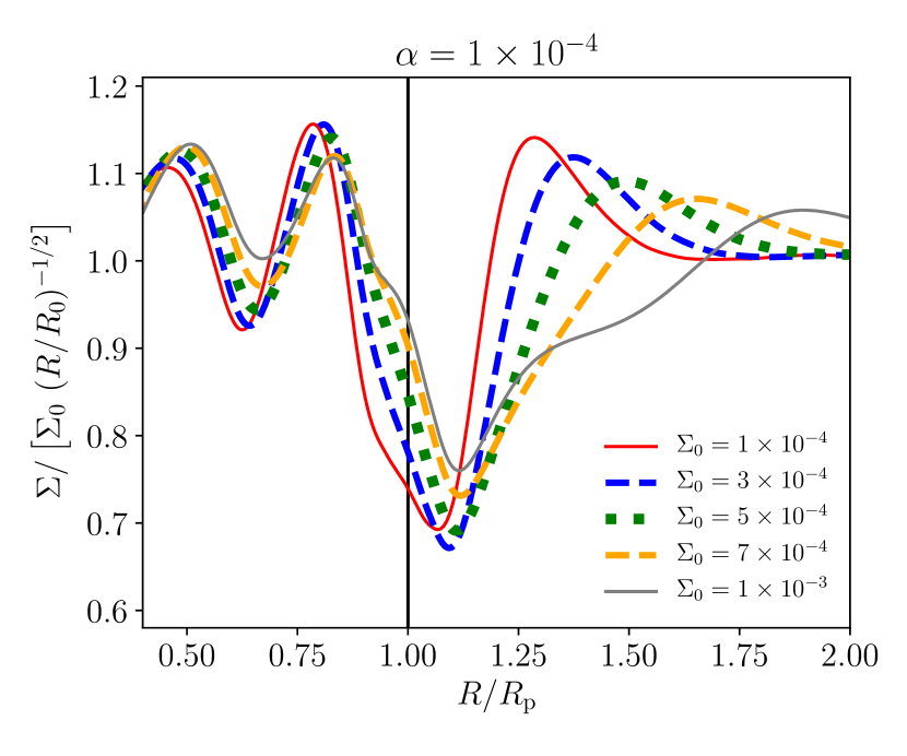
Figure 4: Azimuthally averaged surface density normalized by the initial surface density ($=\Sigma_{0}(R/R_{0})^{-1/2}$) for the cases of $\alpha=10^{-4}$ at $t=1000\ t_{0}$. The planet mass and aspect ratio are the same as those of the case shown in Figure 2.

Dependence of the radial difference between $R_{\rm gap}$ and $R_{\rm p}$ is clearly shown in Figure 4 which illustrates the azimuthally averaged surface density normalized by $R^{-1/2}$ for various values of $\Sigma_{0}$. The planet mass, aspect ratio, and the viscosity are the same as those in the case shown in Figure 2. The location with the smallest $\Sigma/\Sigma_{\rm un}$ in the outer disk of the planet corresponds to $R_{\rm gap}$ (see Figure 1). As can be seen from Figure 4, the difference between $R_{\rm gap}$ and $R_{\rm p}$ becomes larger, with the larger $\Sigma_{0}$. When $\Sigma_{0}=10^{-4}$, the planet locates close to the location of the gap bottom. On the other hand, the planet locates at the inner edge of the gap and the $R_{\rm p}$ and $R_{\rm gap}$ are significantly different from each other when $\Sigma_{0}=10^{-3}$.

In all the cases shown in Figure 4, a visible secondary gap is formed. The location of the secondary gap weakly depends on $\Sigma_{0}$, namely, it forms at slightly smaller radii with a smaller $\Sigma_{0}$ ($R^{\rm 2nd}_{\rm gap}/R_{\rm p}=0.67$ in the case with $\Sigma_{0}=10^{-3}$, and $R^{\rm 2nd}_{\rm gap}/R_{\rm p}=0.63$ in the case with $\Sigma_{0}=10^{-4}$). The depths of the gap in the vicinity of the planet (primary gap) and the secondary gap hardly depends on $\Sigma_{0}$.

The radial shift between the locations of the planet and the gap depends on the $\alpha$ parameter and the aspect ratio.

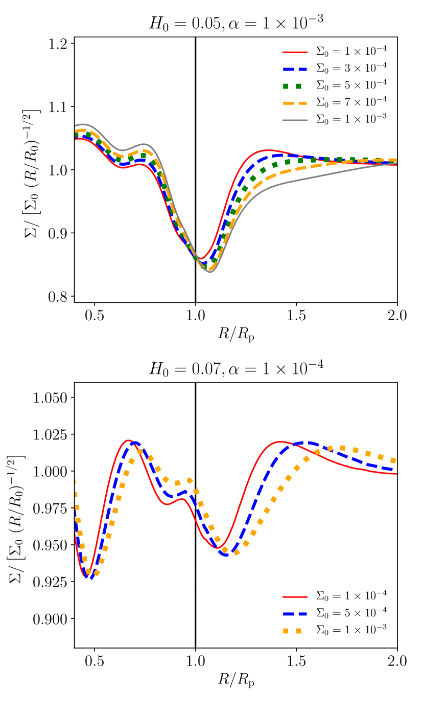
Figure 5: The same as Figure 4, but for the case with $\alpha=10^{-3}$ (upper panel) and for the case with $H_{0}=0.07$.

The upper panel of Figure 5 shows the azimuthally averaged surface density normalized by the initial surface density distribution in the case with $\alpha=10^{-3}$, and the planet mass and aspect ratio are the same as those in the fiducial case. As shown in Figure 5, the radial difference hardly depends on $\Sigma_{0}$ when $\alpha=10^{-3}$. Although the secondary gap is formed in this case at $R/R_{\rm p}=0.64$, moreover, it is not visible because its depth is very shallow. The lower panel of Figure 5 shows the case with $H_{0}=0.07$. Even when the aspect ratio is larger than that in the fiducial case, the radial difference between $R_{\rm p}$ and $R_{\rm gap}$ becomes larger with the larger $\Sigma_{0}$, which is the same as that shown in Figure 4. Although the gap around the planet (primary gap) is shallower than that in the case of Figure 4 due to the larger $H_{0}$, the depth of the secondary gap is similar to that in the case shown in Figure 4. The location of the secondary gap is formed at the smaller radii ($R/R_{\rm p}\simeq 0.5$) than that in the case shown in Figure 4. In Section 3.3, we discuss the parameter dependence of the secondary gap.

3.2 Empirical formula for the radial shift between the locations of the planet and the gap

3.2.1 Timescales

As shown in the previous subsections, the radial difference between the locations of the planet and the gap becomes larger with the lower viscosity and higher surface density. This radial difference may be explained by the ratio of the timescales of the gap formation and the radial migration. According to Kanagawa et al. (2017a), the timescale of the gap formation $t_{\rm gap}$ is

$$t_{\rm gap} =\left(\frac{\Delta_{\rm gap}}{2R_{\rm p}}\right)^{2}\left(\frac{h_{\rm p}}{R_{\rm p}}\right)^{-2}\alpha^{-1}\Omega_{\rm K,p}^{-1},$$ (6)

where $\Delta_{\rm gap}$ is the half width of the gap which can be given by

$$\frac{\Delta_{\rm gap}}{R_{\rm p}} =0.41K^{\prime 1/4},$$ (7)

$$K^{\prime} =\left(\frac{M_{\rm p}}{M_{\ast}}\right)^{2}\left(\frac{h_{\rm p}}{R_{\rm p}}\right)^{-3}\alpha^{-1},$$ (8)

where $\Omega_{\rm K}$ denote the Keperian angular velocity, and the subscription ’p’ indicates the value at $R=R_{\rm p}$. Equation (6) can be rewritten as

$$t_{\rm gap} =4.24\left(\frac{M_{\rm p}/M_{\ast}}{5\times 10^{-5}}\right)\left(\frac{h_{\rm p}/R_{\rm p}}{0.05}\right)^{-7/2}$$

$$\quad\times\left(\frac{\alpha}{10^{-4}}\right)^{-3/2}\left(\frac{M_{\ast}}{1M_{\odot}}\right)^{-1/2}\left(\frac{R_{\rm p}}{50\ \mbox{AU}}\right)^{3/2}\ \mbox{Myr}$$ (9)

When the radial migration is progressing slower than its gap formation, the gap shape can reach that in steady state before the planet moves significantly. In this case, the migration timescale $t_{\rm mig}{}_{\rm,steady}$ can be given by (Kanagawa et al., 2018b),

$$t_{\rm mig}{}_{\rm,steady} =\frac{\Sigma_{\rm un,p}}{\Sigma_{\rm gap}}\tau_{I},$$

$$=\left(1+0.04K\right)\tau_{I}$$ (10)

where $\Sigma_{\rm un,p}$ is the unperturbed surface density at $R_{\rm p}$ and $K$ is defined by

$$K =\left(\frac{M_{\rm p}}{M_{\ast}}\right)^{2}\left(\frac{h_{\rm p}}{R_{\rm p}}\right)^{-5}\alpha^{-1},$$ (11)

and $\Sigma_{\rm gap}$ is the surface density at the bottom of the gap in steady state:

$$\frac{\Sigma_{\rm gap}}{\Sigma_{\rm un,p}} =\frac{1}{1+0.04K}.$$ (12)

The migration timescale predicted by the type I migration $\tau_{I}$ is expressed by (Tanaka et al., 2002; Paardekooper et al., 2010)

$$\tau_{I} =\frac{1}{2c}\left(\frac{M_{\rm p}}{M_{\ast}}\right)^{-1}\left(\frac{M_{\ast}}{\Sigma_{\rm un,p}R_{\rm p}^{2}}\right)\left(\frac{h_{\rm p}}{R_{\rm p}}\right)^{2}\Omega_{\rm K,p}^{-1},$$ (13)

$$=1.68\left(\frac{c}{3}\right)\left(\frac{M_{\rm p}/M_{\ast}}{5\times 10^{-5}}\right)^{-1}\left(\frac{\Sigma_{\rm un,p}}{1\mbox{ g/cm}^{2}}\right)^{-1}$$

$$\qquad\left(\frac{h_{\rm p}/R_{\rm p}}{0.05}\right)^{2}\left(\frac{M_{\ast}}{1M_{\odot}}\right)^{1/2}\left(\frac{R_{\rm p}}{50\mbox{ AU}}\right)^{1/2}\mbox{ Myr},$$ (14)

where the coefficient $c$ is related to the radial distributions of $\Sigma$ and $h$, here we adopt $c=3$. When $t_{\rm gap}$ is much longer than $1000\ t_{0}$, the migration timescale can not reach the value in steady state, which is given by Equation (10).

When the viscosity is very low as in the case we assume in this paper, the gap-opening time is much longer than the migration timescale given by Equation (10). In this case, the planet migrates with a gap which is not fully formed and the migration timescale must be shorter than that given by Equation (10), due to the incomplete gap formation. Considering this effect of the incomplete formation of the gap, Kanagawa et al. (2018b) also gives the following formula:

$$t_{\rm mig} =\left[1+0.04K\left(1-e^{-t/t_{\rm gap}}\right)\right]\tau_{I}.$$ (15)

In particular, the migration timescale is approximately given by $\tau_{I}$ during $1000t_{0}$ (our simulation time) when the viscosity is very small, namely $\alpha\sim 1\times 10^{-4}$, since $t_{\rm gap}\gg 1000t_{0}$.

3.2.2 Empirical formula

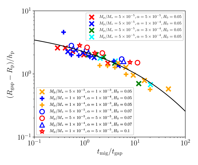
Figure 6: Radial shift ($\Delta$) between the planetary position ($R_{\rm p}$) to the location of the gap ($R_{\rm gap}$) for various planet masses, $\alpha$ and $\Sigma_{0}$. The thin solid line denotes our empirical formula (Equation 16).

We estimate the gap-opening timescale $t_{\rm gap}$ by Equation (6) and the migration timescale $t_{\rm mig}$ by Equation (15). Figure 6 shows the radial difference between the locations of the planet and the gap, as a function of the ratio of $t_{\rm mig}$ and $t_{\rm gap}$. As can be seen from the figure, the shift can be fitted by the following empirical formula as a function of $t_{\rm mig}/t_{\rm gap}$, as

$$\frac{R_{\rm gap}-R_{\rm p}}{h_{\rm p}} =6.05\exp\left[-\left(\frac{t_{\rm mig}}{t_{\rm gap}}\right)^{0.25}\right].$$ (16)

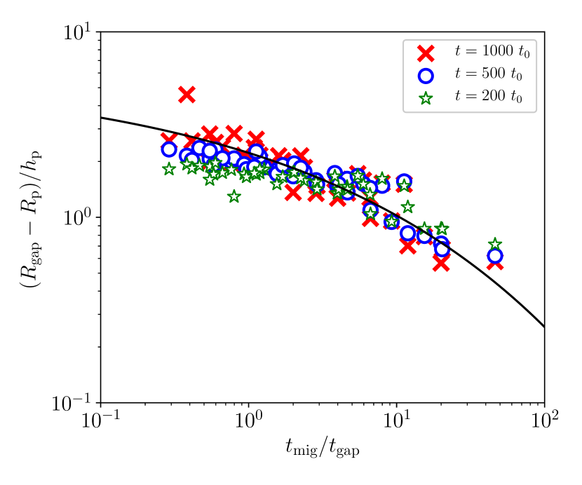
Figure 7: The same as Figure 6, but for different moments, $t=200\ t_{0}$ (0.2 Myr when $R_{0}=100$ AU), $t=500t_{0}$ (0.5 Myr) and $t=1000t_{0}$ (1 Myr shown in Figure 6).

In Figure 7, we show the relation between the radial difference between $R_{\rm p}$ and $R_{\rm gap}$ at the different moments. As can be seen from the figure, the scaling relation given by Equation (16) is still valid, regardless of the time. This result implies that Equation (16) can be applied to protoplanetary disks, regardless of the evolution phases, from Class I to Class II. Observational implications of Equation (16) is discussed in Section 4.2.

3.3 Secondary gap

When the viscosity is relatively low, the planet can form the secondary gap in the inner disk of the planet (e.g., Bae et al., 2017; Dong et al., 2017). From the depth and the location of the secondary gap, we can constrain the viscosity and the scale height.

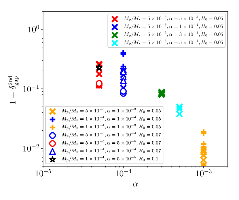
Figure 8: Depths of the secondary gap for various runs at $t=1000\ t_{0}$.

In Figure 8, we illustrate the depth of the secondary gaps given by our simulations ($\delta_{\rm gap}^{\rm 2nd}$) at $t=1000\ t_{0}$. When the $\alpha$-parameter is relatively large as $\sim 10^{-3}$, only the shallow gap is formed. In this case, the secondary gap could not be observed. On the other hand, in the case with the low viscosity, namely $\alpha\lesssim 3\times 10^{-4}$, the relatively deep gap is formed, namely $\delta_{\rm gap}^{\rm 2nd}\lesssim 0.9$. For $\alpha\lesssim 3\times 10^{-4}$, the depth of the secondary gap is not sensitive to $\alpha$. Hence, we can obtain the constraint of $\alpha\lesssim 3\times 10^{-4}$ if the secondary gap is observed. Otherwise, we can constrain the lower limit as $\alpha\gtrsim 3\times 10^{-4}$.

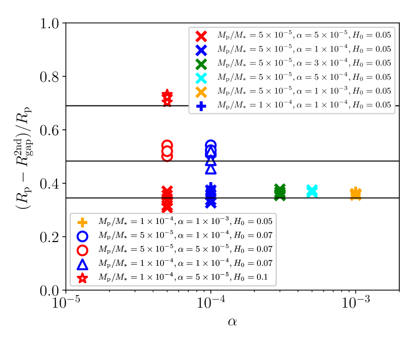
Figure 9: Locations of the secondary gap at $t=1000\ t_{0}$. The solid lines indicate Equation (17) with $(h/R)^{\rm 2nd}_{\rm gap}=0.05$, $0.07$, and $0.1$ from the bottom. Note that in the cases shown in this figure, the aspect ratio is constant throughout the computational domain.

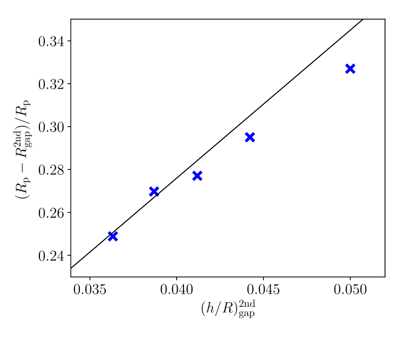
Figure 10: Location of the secondary gap at $t=1000\ t_{0}$ as a function of the aspect ratios at the secondary gap when the aspect ratio depends on radii, $h/R=H_{0}(R/R_{0})^{f}$. From the left, the crosses correspond to the cases of $f=0.5$, $f=0.35$, $f=0.25$, $f=0.15$, and $f=0$, respectively. The planet mass, the value of $\alpha$-parameter, the disk aspect ratio at $R=R_{0}$ are the same as those in our fiducial case. The solid line denotes Equation (17).

Figure 9 illustrates the locations of the secondary gap. As different from the dependence of $\delta_{\rm gap}^{\rm 2nd}$, the location does not depend on $\alpha$. We found that $R_{\rm gap}^{\rm 2nd}-R_{\rm p}$ is proportional to $H_{0}$. The location of the secondary gap also depends on a radial distribution of the aspect ratio. To investigate effects of the radial distribution of the aspect ratio, assuming the $h/R=H_{0}(R/R_{0})^{f}$, we carried out additional hydrodynamic simulations with different values of $f$ ($f=0.15,0.25,0.35,0.5$). The other parameters (e.g., $M_{\rm p},\alpha,H_{0}$) are the same as those of our fiducial case. Results of these simulations are shown in Figure 10. As can be seen from the figure, the location of the secondary gap is proportional to the aspect ratio at the secondary gap $(h/R)_{\rm gap}^{\rm 2nd}$, rather than that at the planetary orbital radius.

Taking into account Figures 9 and 10, we can obtain the relation between the location of the secondary gap and the aspect ratio as

$$\frac{R_{\rm gap}^{\rm 2nd}-R_{\rm p}}{R_{\rm p}}=0.345\left[\frac{(h/R)^{\rm 2nd}_{\rm gap}}{0.05}\right].$$ (17)

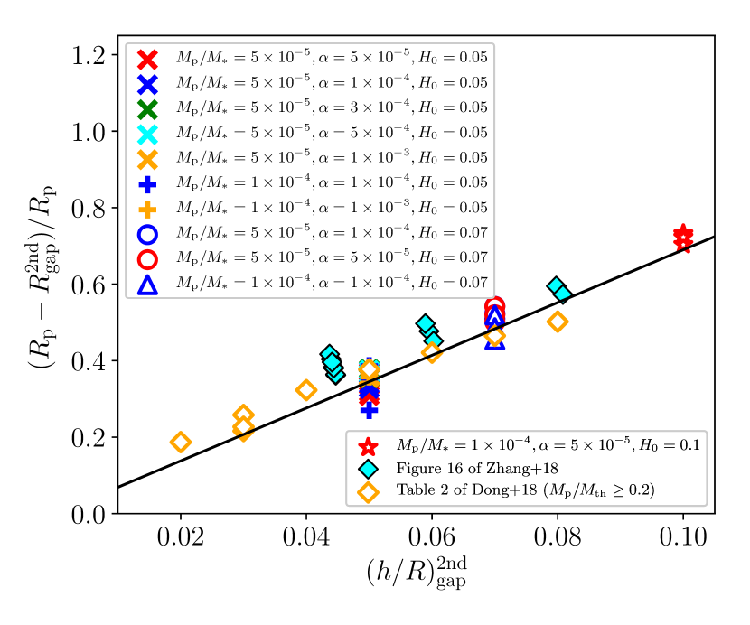
Figure 11: The same as Figure 9, but it is shown by a function of the aspect ratio at the location of the secondary gap. The solid line denotes Equation (17)

Figure 11 shows the same as that shown in Figure 9, but as a function of the aspect ratio at the location of the secondary gap. This figure shows that the fitting formula of Equation (17) also can well reproduce the location of the secondary gap. We should note that the position of the secondary gap also depends on the migration speed, though its dependence is weak as pointed out in Section 3.1. When the migration is slow in the case with a smaller $\Sigma_{0}$, $1-R_{\rm gap}^{\rm 2nd}/R_{\rm p}$ is slightly larger. Because of it, the locations of the secondary gap are spread within the range of $\sim 0.1R_{\rm p}$ in Figure 11 even when the mass of the planet, aspect ratio and viscosity are the same. We also confirmed this trend by carrying out the simulation with a fixed orbit. In the case of the planet with a fixed orbit, the value of $1-R_{\rm gap}^{\rm 2nd}/R_{\rm p}$ is almost the same as the upper values shown in Figure 11.

Dong et al. (2018a) and Zhang et al. (2018) have also shown that the location of the secondary gap depends on the disk scale height, and they give similar scaling relations to Equation (17). In Figure 11, we plot the data extracted from Table 2 of Dong et al. (2018a) (data for $M_{\rm p}/M_{\rm th}\geq 0.2$, where $M_{\rm th}=(h_{\rm p}/R_{\rm p})^{3}$) and Figure 16 of Zhang et al. (2018). Equation (17) also can reproduce both the results given by Dong et al. (2018a) and Zhang et al. (2018). In the scaling of Zhang et al. (2018), the power of $h/R$ is smaller than that of Equation (17), namely $R_{\rm p}-R_{\rm gap}^{\rm 2nd}\propto(h/R)^{0.58}$, though it hardly depends on the mass of the planet similar to Equation (17). The difference of the power of $h/R$ could be caused by the spatial distribution of the aspect ratio. Since Zhang et al. (2018) assumes $h/R\propto R^{0.25}$, the aspect ratio at the location of the secondary gap is smaller than that at the location of the planet.

Dong et al. (2018a) assume a constant aspect ratio ($h/R=\mbox{const}$) and gives a similar power of $h/R$, namely $\propto(h/R)^{1.3}$, but it depends on $M_{\rm p}^{0.2}$. The formula given by Dong et al. (2018a) give a better fit when the planet is small, namely $M_{\rm p}/M_{\rm th}\lesssim 0.2$. However, the prediction given by the formula of Dong et al. (2018a) does not fit the results of simulations when $M_{\rm p}/M_{\rm th}\gg 1$ (see Appendix B). For a relatively large planet which can be detected by ALMA, Equation (17) may be convenient, rather than the formula given by Dong et al. (2018a).

4 Discussion

4.1 Feasibility of observations

In the above section, we show that when the inward migration of the planet is faster than the gap-opening, the orbital radius of the planet $R_{\rm p}$ is smaller than that of the gap $R_{\rm gap}$. If such a difference is observed, it could be evidence that the planet is formed in the outer region and it is migrating inward quickly. We also found the scaling relation of Equation (16) which gives the relation of the radial difference between $R_{\rm p}$ and $R_{\rm gap}$ and the ratio of the timescale of the migration and gap-opening given by Equations (15) and (6), respectively. If the secondary gap is observed, we also can constrain the disk viscosity and aspect ratio as shown in Section 3.3. In this subsection, we discuss feasibility of the observations of gap profile of gas and excess of the dust emission from a planet embedded within the disk.

The CO line emission has been detected by the observation with ALMA in Band 7 in Cycle 2 at the disk around TW Hya (Nomura et al., 2016). By using the line emission from ¹³CO and C¹⁸O J= 3–2, Nomura et al. (2016) has obtained the column density distribution of CO. Since the C¹⁸O emission is likely to be optically thin in an outer region of the disk, the CO column density can be directly compared with the gas surface density given by hydrodynamic simulations . In the recent observation with higher angular resolution ($\sim$ 0.15 arcsec, $\sim 9$ AU resolution) and 2.3 hours on-source integration time, the gap profile of CO is possibly detected around $\sim 50$ AU (Nomura et al. in prep). With ALMA in Band 7 in Cycle 3, Tsukagoshi et al. (2019) has detected the point source in dust continuum emission at $52$ AU in the disk around TW Hya. The angular resolution and the on-source integration time of that observation are $\sim$ 0.043 arcsec ($\sim 3$ AU resolution) and 3.5 hours, respectively.

In the basis of the observations of TW Hya mentioned above, we estimate feasibility of the detection of CO and dust point source in other protoplanetary disks. We assume that a distance to the protoplanetary disk is around $130$pc in this estimate (the distance to TW Hya is about $60$pc). Because of the larger distance, it takes higher angular resolution and longer integration time to detect the CO line and a point source in dust emission. To achieve the same spatial resolutions of Nomura et al. (2016) and Tsukagoshi et al. (2019), the angular resolution of $0.07$ arcsec for CO line observation and $0.023$ arcsec for the dust continuum observation are required. Since a required integration time is proportional to 4th power of the angular resolution, it can be estimated as $\sim 50$  hours, which is unreasonably long at the current moment. However, since the gap width is scaled by the orbital radius of the planet (see e.g., Kanagawa et al., 2016), the gap profile can be detected in an outer region with lower angular resolution. When $R_{\rm p}\sim 100$ AU, one could observe the gap of CO emission and the point source of the dust emission with the similar angular resolutions and integration times, for the disk with the distance of $\simeq 130$pc.

In the outer region ($\sim 100$ AU), the CO column density and the temperature may be smaller and lower than these of TW Hya at $\sim 50$ AU. With lower CO column density and temperature, a longer integration time would be required due to weak emission. For instance, however, Isella et al. (2016) has shown that in the case of the disk around HD 163296, the C¹⁸O J = 2–1 emission at $100$ AU ($\sim 0.65$ Jy/arcsec²/(km/s)) is comparable to the C¹⁸O J= 3–2 emission at $50$ AU in the disk of TW Hya ($\sim 0.14$ Jy/arcsec²/(km/s)). Moreover, DSHARP program has observed the ¹² CO J= 2–1 emission and revealed that in some disks, i.e., AS 209 (Guzmán et al., 2018) and HD 143006 (Pérez et al., 2018), the ¹² CO emission around 100 AU is comparable with or larger than the C¹⁸O emission at 50 AU in TW Hya disk. For the disks around Herbig stars, the CO emission at $100$ AU can be comparable with that at $50$ AU in the disk around TW Hya. The gap in the CO emission and the point source in the dust emission could be observed with the similar angular resolutions and integration times as these of Nomura et al. (2016) and Tsukagoshi et al. (2019).

Detecting the secondary gap in the gas might be challenging because it is shallow and narrow, moreover formed in an inner region than the primary gap. However, the secondary gap is easier to be observed by the observations of the dust continuum. We can estimate the disk scale height from the location of the secondary gap measured by the location of the secondary gap by dust observations, by Equation (17). The depth of the secondary gap could be affected by the size of the dust grains, as well as the gas viscosity. Hence, we need to take care of the size of the dust to estimate the upper/lower limit of viscosity.

4.2 Observational implications

In this subsection , we discuss what can constrained when the gap and planet are observed. The difference between $R_{\rm p}$ and $R_{\rm gap}$ depends on $t_{\rm mig}/t_{\rm gap}$, that is, it depends on the mass of the planet, the disk viscosity, aspect ratio and the gas surface density of the disk, as can be seen from Equation (16). The mass of the planet can be estimated from the excess of the flux at the planet location (e.g., Ayliffe & Bate, 2009; Wang et al., 2014; Szulágyi et al., 2018), and the aspect ratio can be also estimated from the brightness temperature of the dust emission if the dust emission is detected (e.g., Nomura et al., 2016). On the other hand, the viscosity and the gas surface density (not dust and CO densities) are relatively difficult to be constrained from the observation. However, by using Equation (16), we can constrain the viscosity and the gas surface density from the observed radial difference between $R_{\rm p}$ and $R_{\rm gap}$.

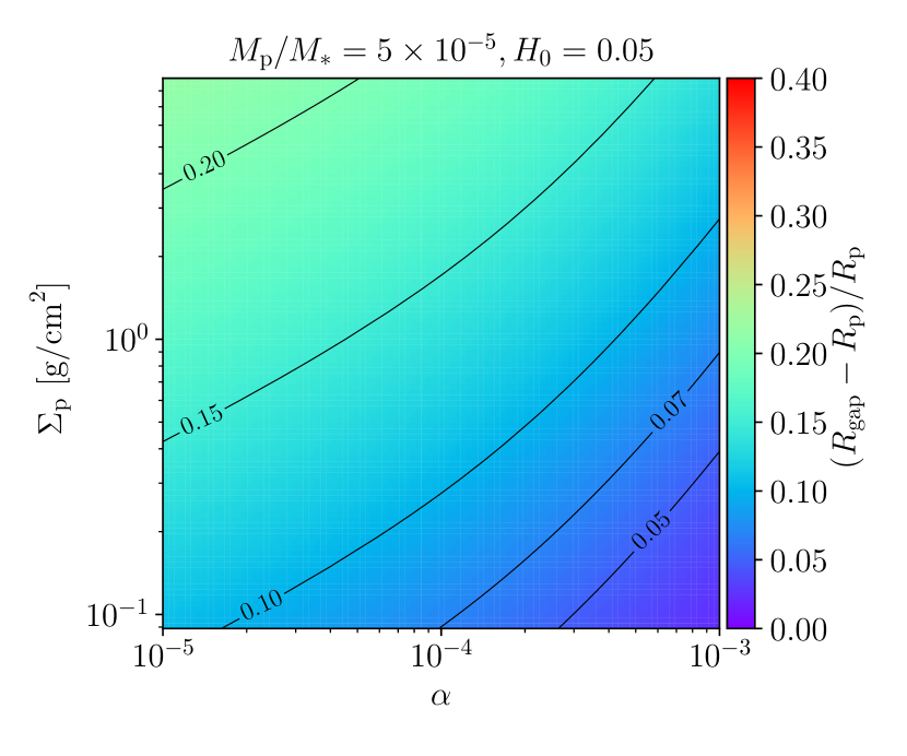
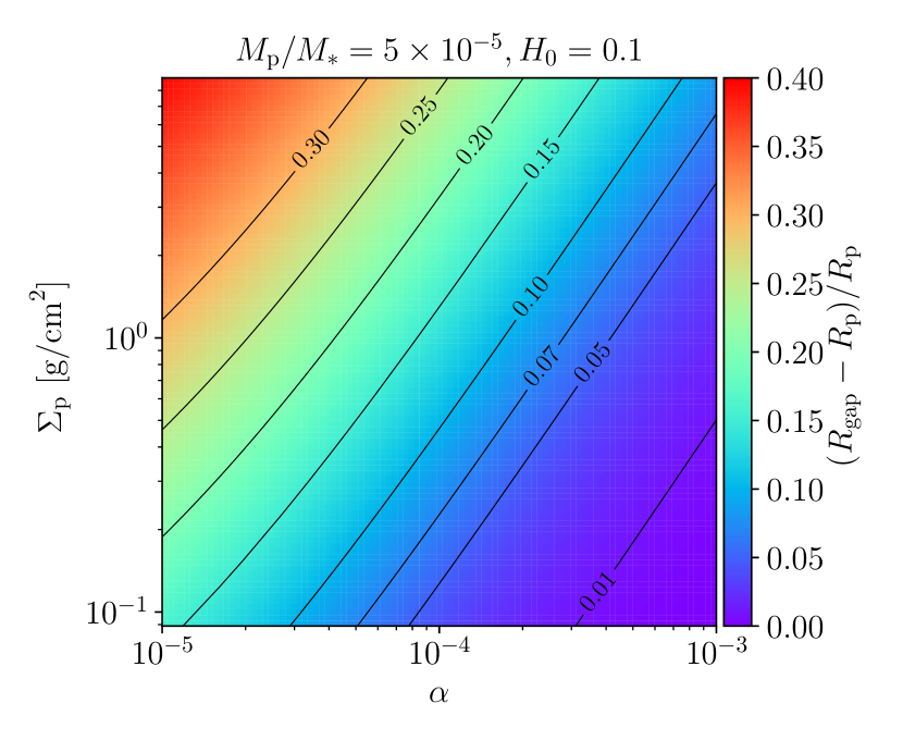
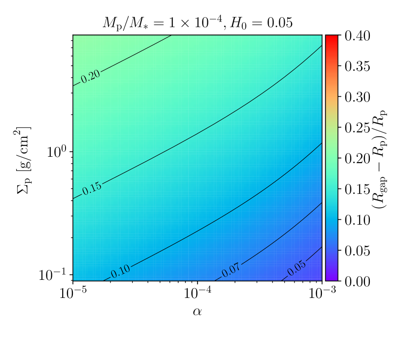
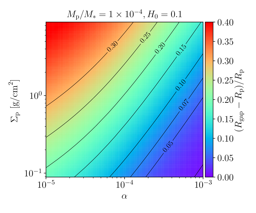
Figure 12: Radial difference between $R_{\rm p}$ and $R_{\rm gap}$ as a function of the viscosity $\alpha$ and the gas surface density $\Sigma_{\rm un,p}$. The planet mass is $M_{\rm p}/M_{\ast}=5\times 10^{-5}$ (Neptune size) in the upper raw, and $M_{\rm p}/M_{\ast}=1\times 10^{-4}$ in the lower raw, respectively, and we also assume $M_{\ast}=1M_{\odot}$ and $R_{0}=100$ AU in the figures. The disk aspect ratio is $0.05$ in the left column and $H_{0}=0.1$ in the right column, respectively.

Figure 12 shows that the radial difference between $R_{\rm p}$ and $R_{\rm gap}$ as a function of $\alpha$ and $\Sigma_{\rm un,p}$ with the given planet masses ($M_{\rm p}/M_{\ast}=5\times 10^{-5}$ in the upper panels and $M_{\rm p}/M_{\ast}=1\times 10^{-4}$ in the lower panels) and aspect ratios ($H_{0}=0.05$ in the left panels and $H_{0}=0.1$ in the right panels). When the difference between $R_{\rm p}$ and $R_{\rm gap}$ is measured from the observation, we can constrain $\alpha$ and $\Sigma_{0}$ along the line corresponding to be the observed value of $R_{\rm p}-R_{\rm gap}$ in Figure 12. As can be seen from the figure, the difference between $R_{\rm p}$ and $R_{\rm gap}$ is relatively sensitive on $H_{0}$, whereas it does not significantly depend on the mass of the planet.

In addition to the difference between $R_{\rm p}$ and $R_{\rm gap}$, we may constrain the viscosity and the disk aspect ratio from the secondary gap formed in the inner disk, as shown in Section 3.3. When the visible secondary gap is observed, we can give the upper limit of the $\alpha$-parameter, namely $\alpha\lesssim 3\times 10^{-4}$, in the vicinity of the planet. When no secondary gap is observed, on the other hand, we can give the lower limit of the $\alpha$-parameter as $\alpha\gtrsim 3\times 10^{-4}$. Moreover, if the secondary gap is observed, the aspect ratio can be estimated from the location of the secondary gap by Equation (17), which is an independent constraint from that by dust/gas emissions. With the upper/lower limit of $\alpha$ and the constraint of the disk aspect ratio from the depth and the location of the secondary gap, we can more accurately estimate the viscosity and, especially the gas surface density from Figure 12.

4.3 Caveat of our model

In this paper, we adopt the simple locally isothermal equation of state (EoS). However, recently Miranda & Rafikov (2019) shows that simulations with the locally isothermal EoS can overestimate the contrast of ring and gaps features, as compared with results given by simulations with adiabatic EoS, even when the adiabatic index is $1.001$. As can be seen from Figure 2 of Miranda & Rafikov (2019), this discrepancy becomes significant for the gap and ring structures formed by a relatively large dust grains ($St\gtrsim 0.01$). For the gas structures, the location of the primary and secondary gaps do not change much between locally isothermal EoS and adiabatic EoS cases. In this paper, we consider the primary and secondary gaps. Hence, our results would not be significantly affected in the adiabatic disk with the adiabatic index being $1.001$.

In the adiabatic disk, the torque exerted on the planet (especially the horseshoe torque) can be different from that in the locally isothermal disk (e.g., Paardekooper et al., 2010). The migration velocity of the planet in the adiabatic disk can be slower than that in the locally isothermal disk (e.g., Bitsch et al., 2015a). The non-isothermal effects may affect the gap structure, though it may not be significant (Kley & Crida, 2008). However, in an outer region where is optically thin, the cooling can be efficient. In this case, the isothermal EoS could be good approximation.

The torque exerted from the large dust grains (so-called pebbles) can significantly slow the inward planetary migration down due to an asymmetric distribution of pebbles, as discussed by Benítez-Llambay & Pessah (2018). However, when the planet forms gap and the mass of the planet is larger than the so-call pebble-isolation mass (e.g., Morbidelli & Nesvorny, 2012; Lambrechts et al., 2014; Bitsch et al., 2018), such large dust grains cannot reach the vicinity of the planet. In this case, the planet hardly feels the torque exerted from the pebble. When the mass of the planet is larger than the pebble-isolation mass, the pebbles accumulate at an outer edge of the gap. Since the surface density of the gas at the outer edge decreases due to the feedback from the pebbles accumulated at the outer edge, the inward migration of the planet also significantly slows down or change a direction of the migration (Kanagawa, 2019). However, this effects is significant when an amount of the pebbles are accumulated at the outer edge by catching up with the planet. When the inward migration of the planet is fast, this effect may be inefficient since the relative speed between the pebble and the planet is not large enough.

If an actual migration velocity is deviated from that given by Equation (15), we could overestimate/underestimate the surface density of gas around the planet. This overestimate/underestimate could be found by comparing with the CO density estimated by the CO emission, though the CO density also has uncertainties related to e.g., CO/H ratio.

In the parameter range that we investigated in this paper, the planet migrates only inward. However, several mechanisms discussed above may change the migration speed and let the planetary migration outward. Even when the outward migration, the location of the planet and the gap could be shifted. In this case, the planet would be detected at the outer edge of the gap and thus $R_{\rm p}>R_{\rm gap}$.

5 Summary

We investigated effects of the fast inward migrating planet on the shape of the gap in the protoplanetary disk when both the planet and the gap are observed, by carrying out hydrodynamic simulations. Our results are summarized as follows:

1. we found that the orbital radius of the planet ($R_{\rm p}$) can be shifted inward from the location of the gap ($R_{\rm gap}$). When the radial shift between the locations of the planet and the gap is observed, it can be evidence that the planet is formed in the outer region and migrating to the inner region quickly.

2. We also derived the empirical formula between the radial shift of $R_{\rm p}$ and $R_{\rm gap}$ and the ratio of the migration and gap-opening timescales (Equation 16). The radial difference between $R_{\rm p}$ and $R_{\rm gap}$ becomes larger as the migration timescale is shorter than the timescale of the gap-opening.

3. Since the ratio of the timescales of the migration and the gap-opening is a function of the planet mass and disk parameters (gas surface density, aspect ratio, viscosity), we can constrain these quantities (especially the viscosity and the gas surface density) from the observation, by using Equation (16).

4. When the viscosity is relatively low, the secondary gap can be formed in the inner disk. The depth and location of the secondary gap depends on the viscosity and the aspect ratio, respectively (Figures 8 and 9). If the secondary gap is observed, we can constraint the viscosity as $\alpha\lesssim 3\times 10^{-4}$. Otherwise, we can obtain the lower limit of the viscosity as $\alpha\gtrsim 3\times 10^{-4}$. The secondary gap is formed in a more inner part with a larger disk aspect ratio (Equation 17). By using these constraints from the secondary gap, we can further estimate the parameters in the planet formation region.

Appendix A Resolution dependence

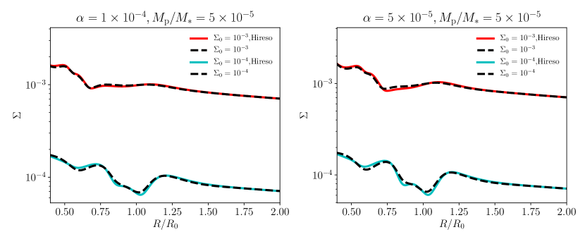
Figure 13: Azimuthally averaged surface density distributions at $t=1000\ t_{0}$, when $M_{\rm p}/M_{\ast}=5\times 10^{-5}$, $H_{0}=0.05$. In the left panel, $\alpha=1\times 10^{-4}$ and in the right panel, $\alpha=5\times 10^{-5}$. The solid lines indicate the results given by the simulations with the high-resolution ($N_{r}=1024,N_{\phi}=2048$) and the dashed lines indicate the results given by the simulations with the standard resolution ($N_{r}=512,N_{\phi}=1024$).

In this appendix, we discuss resolution convergence of our results. We carried out hydrodynamic simulations with higher resolution (1024 and 2048 meshes in radial and azimuthal directions, respectively) as compared with our standard resolution (512 and 1024 meshes in radial and azimuthal direction, respectively). In Figure 13, we compare the azimuthally averaged surface density at $t=1000\ t_{0}$ with the cases of the high-resolution and the standard resolution, when $M_{\rm p}/M_{\ast}=5\times 10^{-5}$, $H_{0}=0.05$ and $\alpha=1\times 10^{-4}$ (left panel) and $\alpha=5\times 10^{-5}$ (right panel). One can confirm that the surface density distributions are almost converged.

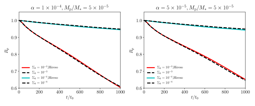
Figure 14: Comparison of evolution of the orbital radius of the planet given by the simulations with the high-resolution and standard resolution. The solid and dashed lines represent the results given by the simulations with the high-resolution and the standard resolution, respectively.

In Figure 14, we compare the evolution of the orbital radius of the planet given by the simulations with the high-resolution and the standard resolution. The evolution of the orbital radius is also quite similar to each other, in the cases of the high-resolution and the standard resolution.

Appendix B Location of the secondary gap

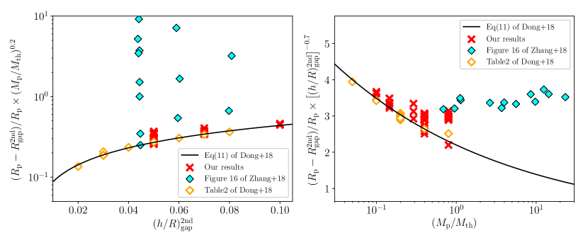
Figure 15: The same as Figure 11, but the axes are different. Moreover, we plot all the data of Dong et al. (2018a) including these for $M_{\rm p}/M_{\rm th}<0.2$. The red crosses, cyan diamonds, and orange diamonds represent the data given by this paper, Zhang et al. (2018) and Dong et al. (2018a), respectively. The solid line indicates the empirical formula given by Dong et al. (2018a).

Dong et al. (2018a) obtains the empirical formula as (Equation 11 of that paper)

$$\frac{R_{\rm gap}^{\rm 2nd}-R_{\rm p}}{R_{\rm p}} =0.27\left(\frac{M_{\rm p}}{M_{\rm th}}\right)^{-0.2}\left[\frac{(h/R)^{\rm 2nd}_{\rm gap}}{0.05}\right]^{0.7}.$$ (B1)

Since $M_{\rm th}=(h_{\rm p}/R_{\rm p})^{3}$, Equation (B1) depends on $(h/R)^{1.3}$ (where we neglect spatial distribution of $h/R$ for simplicity). In Figure 15, we compare the data given by our simulations, Dong et al. (2018a) and Zhang et al. (2018) with Equation (B1). In the left panel, we show the dependence of $h/R$. Equation (B1) well reproduces the results of Dong et al. (2018a) and ours, but it does not match to the results given by Zhang et al. (2018). In the right panel of Figure 15, we show the dependence of $M_{\rm p}/M_{\rm th}$. Our results are consistent with the prediction given by Equation (B1) when $M_{\rm p}/M_{\rm th}\lesssim 0.3$. As $M_{\rm p}/M_{\rm th}$ increases, the results given by our simulations deviates from the prediction given by Equation (B1). Since Zhang et al. (2018) investigated a large planet, namely $M_{\rm p}/M_{\rm th}\gtrsim 1$, Equation (B1) cannot reproduce these data.

References

- Akiyama et al. (2015) Akiyama, E., Muto, T., Kusakabe, N., et al. 2015, ApJ, 802, L17, doi: 10.1088/2041-8205/802/2/L17
- ALMA Partnership et al. (2015) ALMA Partnership, Brogan, C. L., Pérez, L. M., et al. 2015, ApJ, 808, L3, doi: 10.1088/2041-8205/808/1/L3
- Ayliffe & Bate (2009) Ayliffe, B. A., & Bate, M. R. 2009, MNRAS, 397, 657, doi: 10.1111/j.1365-2966.2009.15002.x
- Bae et al. (2017) Bae, J., Zhu, Z., & Hartmann, L. 2017, ApJ, 850, 201, doi: 10.3847/1538-4357/aa9705
- Benítez-Llambay & Pessah (2018) Benítez-Llambay, P., & Pessah, M. E. 2018, ApJ, 855, L28, doi: 10.3847/2041-8213/aab2ae
- Bitsch et al. (2015a) Bitsch, B., Johansen, A., Lambrechts, M., & Morbidelli, A. 2015a, A&A, 575, A28, doi: 10.1051/0004-6361/201424964
- Bitsch et al. (2015b) Bitsch, B., Lambrechts, M., & Johansen, A. 2015b, A&A, 582, A112, doi: 10.1051/0004-6361/201526463
- Bitsch et al. (2018) Bitsch, B., Morbidelli, A., Johansen, A., et al. 2018, A&A, 612, A30, doi: 10.1051/0004-6361/201731931
- Bryden et al. (1999) Bryden, G., Chen, X., Lin, D. N. C., Nelson, R. P., & Papaloizou, J. C. B. 1999, ApJ, 514, 344, doi: 10.1086/306917
- Crida & Morbidelli (2007) Crida, A., & Morbidelli, A. 2007, MNRAS, 377, 1324, doi: 10.1111/j.1365-2966.2007.11704.x
- D’Angelo et al. (2003) D’Angelo, G., Kley, W., & Henning, T. 2003, ApJ, 586, 540, doi: 10.1086/367555
- de Val-Borro et al. (2006) de Val-Borro, M., Edgar, R. G., Artymowicz, P., et al. 2006, MNRAS, 370, 529, doi: 10.1111/j.1365-2966.2006.10488.x
- Dipierro et al. (2015) Dipierro, G., Price, D., Laibe, G., et al. 2015, MNRAS, 453, L73, doi: 10.1093/mnrasl/slv105
- Dong & Fung (2017) Dong, R., & Fung, J. 2017, ApJ, 835, 146, doi: 10.3847/1538-4357/835/2/146
- Dong et al. (2017) Dong, R., Li, S., Chiang, E., & Li, H. 2017, ApJ, 843, 127, doi: 10.3847/1538-4357/aa72f2
- Dong et al. (2018a) —. 2018a, ApJ, 866, 110, doi: 10.3847/1538-4357/aadadd
- Dong et al. (2015) Dong, R., Zhu, Z., & Whitney, B. 2015, ApJ, 809, 93, doi: 10.1088/0004-637X/809/1/93
- Dong et al. (2018b) Dong, R., Liu, S.-y., Eisner, J., et al. 2018b, ApJ, 860, 124, doi: 10.3847/1538-4357/aac6cb
- Dürmann & Kley (2015) Dürmann, C., & Kley, W. 2015, A&A, 574, A52, doi: 10.1051/0004-6361/201424837
- Dürmann & Kley (2017) —. 2017, A&A, 598, A80, doi: 10.1051/0004-6361/201629074
- Edgar (2007) Edgar, R. G. 2007, ApJ, 663, 1325, doi: 10.1086/518591
- Fedele et al. (2017) Fedele, D., Carney, M., Hogerheijde, M. R., et al. 2017, A&A, 600, A72, doi: 10.1051/0004-6361/201629860
- Flaherty et al. (2015) Flaherty, K. M., Hughes, A. M., Rosenfeld, K. A., et al. 2015, ApJ, 813, 99, doi: 10.1088/0004-637X/813/2/99
- Flaherty et al. (2018) Flaherty, K. M., Hughes, A. M., Teague, R., et al. 2018, ApJ, 856, 117, doi: 10.3847/1538-4357/aab615
- Flaherty et al. (2017) Flaherty, K. M., Hughes, A. M., Rose, S. C., et al. 2017, ApJ, 843, 150, doi: 10.3847/1538-4357/aa79f9
- Fukagawa et al. (2013) Fukagawa, M., Tsukagoshi, T., Momose, M., et al. 2013, PASJ, 65, L14, doi: 10.1093/pasj/65.6.L14
- Goldreich & Tremaine (1980) Goldreich, P., & Tremaine, S. 1980, ApJ, 241, 425, doi: 10.1086/158356
- Guzmán et al. (2018) Guzmán, V. V., Huang, J., Andrews, S. M., et al. 2018, ApJ, 869, L48, doi: 10.3847/2041-8213/aaedae
- Hashimoto et al. (2011) Hashimoto, J., Tamura, M., Muto, T., et al. 2011, ApJ, 729, L17, doi: 10.1088/2041-8205/729/2/L17
- Hunter (2007) Hunter, J. D. 2007, Computing in Science and Engineering, 9, 90, doi: 10.1109/MCSE.2007.55
- Ida et al. (2013) Ida, S., Lin, D. N. C., & Nagasawa, M. 2013, ApJ, 775, 42, doi: 10.1088/0004-637X/775/1/42
- Ida et al. (2018) Ida, S., Tanaka, H., Johansen, A., Kanagawa, K. D., & Tanigawa, T. 2018, ApJ, 864, 77, doi: 10.3847/1538-4357/aad69c
- Isella et al. (2016) Isella, A., Guidi, G., Testi, L., et al. 2016, Physical Review Letters, 117, 251101, doi: 10.1103/PhysRevLett.117.251101
- Jin et al. (2016) Jin, S., Li, S., Isella, A., Li, H., & Ji, J. 2016, ApJ, 818, 76, doi: 10.3847/0004-637X/818/1/76
- Johansen et al. (2019) Johansen, A., Ida, S., & Brasser, R. 2019, A&A, 622, A202, doi: 10.1051/0004-6361/201834071
- Kanagawa (2019) Kanagawa, K. D. 2019, ApJ, 879, L19, doi: 10.3847/2041-8213/ab2a0f
- Kanagawa et al. (2018a) Kanagawa, K. D., Muto, T., Okuzumi, S., et al. 2018a, ApJ, 868, 48, doi: 10.3847/1538-4357/aae837
- Kanagawa et al. (2015) Kanagawa, K. D., Muto, T., Tanaka, H., et al. 2015, ApJ, 806, L15, doi: 10.1088/2041-8205/806/1/L15
- Kanagawa et al. (2016) —. 2016, PASJ, 68, 43, doi: 10.1093/pasj/psw037
- Kanagawa et al. (2017a) Kanagawa, K. D., Tanaka, H., Muto, T., & Tanigawa, T. 2017a, PASJ, doi: 10.1093/pasj/psx114
- Kanagawa et al. (2018b) Kanagawa, K. D., Tanaka, H., & Szuszkiewicz, E. 2018b, ApJ, 861, 140, doi: 10.3847/1538-4357/aac8d9
- Kanagawa et al. (2017b) Kanagawa, K. D., Ueda, T., Muto, T., & Okuzumi, S. 2017b, ApJ, 844, 142, doi: 10.3847/1538-4357/aa7ca1
- Keppler et al. (2018) Keppler, M., Benisty, M., Müller, A., et al. 2018, A&A, 617, A44, doi: 10.1051/0004-6361/201832957
- Kley (1999) Kley, W. 1999, MNRAS, 303, 696, doi: 10.1046/j.1365-8711.1999.02198.x
- Kley & Crida (2008) Kley, W., & Crida, A. 2008, A&A, 487, L9, doi: 10.1051/0004-6361:200810033
- Lambrechts et al. (2014) Lambrechts, M., Johansen, A., & Morbidelli, A. 2014, A&A, 572, A35, doi: 10.1051/0004-6361/201423814
- Lin & Papaloizou (1979) Lin, D. N. C., & Papaloizou, J. 1979, MNRAS, 186, 799
- Lin & Papaloizou (1986) —. 1986, ApJ, 309, 846, doi: 10.1086/164653
- Long et al. (2018) Long, F., Pinilla, P., Herczeg, G. J., et al. 2018, ApJ, 869, 17, doi: 10.3847/1538-4357/aae8e1
- Lynden-Bell & Pringle (1974) Lynden-Bell, D., & Pringle, J. E. 1974, MNRAS, 168, 603
- Machida et al. (2010) Machida, M. N., Kokubo, E., Inutsuka, S.-I., & Matsumoto, T. 2010, MNRAS, 405, 1227, doi: 10.1111/j.1365-2966.2010.16527.x
- Masset (2000) Masset, F. 2000, A&AS, 141, 165, doi: 10.1051/aas:2000116
- Meru et al. (2019) Meru, F., Rosotti, G. P., Booth, R. A., Nazari, P., & Clarke, C. J. 2019, MNRAS, 482, 3678, doi: 10.1093/mnras/sty2847
- Miranda & Rafikov (2019) Miranda, R., & Rafikov, R. R. 2019, ApJ, 878, L9, doi: 10.3847/2041-8213/ab22a7
- Momose et al. (2015) Momose, M., Morita, A., Fukagawa, M., et al. 2015, PASJ, 67, 83, doi: 10.1093/pasj/psv051
- Morbidelli & Nesvorny (2012) Morbidelli, A., & Nesvorny, D. 2012, A&A, 546, A18, doi: 10.1051/0004-6361/201219824
- Mordasini et al. (2012) Mordasini, C., Alibert, Y., Benz, W., Klahr, H., & Henning, T. 2012, A&A, 541, A97, doi: 10.1051/0004-6361/201117350
- Müller et al. (2018) Müller, A., Keppler, M., Henning, T., et al. 2018, A&A, 617, L2, doi: 10.1051/0004-6361/201833584
- Muto & Inutsuka (2009) Muto, T., & Inutsuka, S.-i. 2009, ApJ, 695, 1132, doi: 10.1088/0004-637X/695/2/1132
- Nazari et al. (2019) Nazari, P., Booth, R. A., Clarke, C. J., et al. 2019, MNRAS, 485, 5914, doi: 10.1093/mnras/stz836
- Nelson et al. (2000) Nelson, R. P., Papaloizou, J. C. B., Masset, F., & Kley, W. 2000, MNRAS, 318, 18, doi: 10.1046/j.1365-8711.2000.03605.x
- Nomura et al. (2016) Nomura, H., Tsukagoshi, T., Kawabe, R., et al. 2016, ApJ, 819, L7, doi: 10.3847/2041-8205/819/1/L7
- Paardekooper et al. (2010) Paardekooper, S.-J., Baruteau, C., Crida, A., & Kley, W. 2010, MNRAS, 401, 1950, doi: 10.1111/j.1365-2966.2009.15782.x
- Paardekooper & Mellema (2004) Paardekooper, S.-J., & Mellema, G. 2004, A&A, 425, L9, doi: 10.1051/0004-6361:200400053
- Pérez et al. (2018) Pérez, L. M., Benisty, M., Andrews, S. M., et al. 2018, ApJ, 869, L50, doi: 10.3847/2041-8213/aaf745
- Pinte et al. (2016) Pinte, C., Dent, W. R. F., Ménard, F., et al. 2016, ApJ, 816, 25, doi: 10.3847/0004-637X/816/1/25
- Rosotti et al. (2016) Rosotti, G. P., Juhasz, A., Booth, R. A., & Clarke, C. J. 2016, MNRAS, 459, 2790, doi: 10.1093/mnras/stw691
- Szulágyi et al. (2018) Szulágyi, J., Cilibrasi, M., & Mayer, L. 2018, ApJ, 868, L13, doi: 10.3847/2041-8213/aaeed6
- Tanaka et al. (2019) Tanaka, H., Murase, K., & Tanigawa, T. 2019, arXiv e-prints, arXiv:1907.02627. https://arxiv.org/abs/1907.02627
- Tanaka et al. (2002) Tanaka, H., Takeuchi, T., & Ward, W. R. 2002, ApJ, 565, 1257, doi: 10.1086/324713
- Tanigawa & Watanabe (2002) Tanigawa, T., & Watanabe, S.-i. 2002, ApJ, 580, 506, doi: 10.1086/343069
- Teague et al. (2016) Teague, R., Guilloteau, S., Semenov, D., et al. 2016, A&A, 592, A49, doi: 10.1051/0004-6361/201628550
- Tsukagoshi et al. (2016) Tsukagoshi, T., Nomura, H., Muto, T., et al. 2016, ApJ, 829, L35, doi: 10.3847/2041-8205/829/2/L35
- Tsukagoshi et al. (2019) Tsukagoshi, T., Muto, T., Nomura, H., et al. 2019, The Astrophysical Journal, 878, L8, doi: 10.3847/2041-8213/ab224c
- van der Marel et al. (2019) van der Marel, N., Dong, R., di Francesco, J., Williams, J. P., & Tobin, J. 2019, ApJ, 872, 112, doi: 10.3847/1538-4357/aafd31
- van der Plas et al. (2017) van der Plas, G., Wright, C. M., Ménard, F., et al. 2017, A&A, 597, A32, doi: 10.1051/0004-6361/201629523
- van der Walt et al. (2011) van der Walt, S., Colbert, S. C., & Varoquaux, G. 2011, Computing in Science and Engineering, 13, 22, doi: 10.1109/MCSE.2011.37
- Wang et al. (2014) Wang, H.-H., Bu, D., Shang, H., & Gu, P.-G. 2014, ApJ, 790, 32, doi: 10.1088/0004-637X/790/1/32
- Weber et al. (2018) Weber, P., Benítez-Llambay, P., Gressel, O., Krapp, L., & Pessah, M. E. 2018, ApJ, 854, 153, doi: 10.3847/1538-4357/aaab63
- Weber et al. (2019) Weber, P., Pérez, S., Benítez-Llambay, P., et al. 2019, ApJ, 884, 178, doi: 10.3847/1538-4357/ab412f
- Winn & Fabrycky (2015) Winn, J. N., & Fabrycky, D. C. 2015, ARA&A, 53, 409, doi: 10.1146/annurev-astro-082214-122246
- Zhang et al. (2018) Zhang, S., Zhu, Z., Huang, J., et al. 2018, ApJ, 869, L47, doi: 10.3847/2041-8213/aaf744
- Zhu et al. (2012) Zhu, Z., Nelson, R. P., Dong, R., Espaillat, C., & Hartmann, L. 2012, ApJ, 755, 6, doi: 10.1088/0004-637X/755/1/6