A queueing system with batch renewal input and negative arrivals

Abstract: This paper studies an infinite buffer single server queueing model with exponentially distributed service times and negative arrivals. The ordinary (positive) customers arrive in batches of random size according to renewal arrival process, and joins the queue/server for service. The negative arrivals are characterized by two independent Poisson arrival processes, a negative customer which removes the positive customer undergoing service, if any, and a disaster which makes the system empty by simultaneously removing all the positive customers present in the system. Using the supplementary variable technique and difference equation method we obtain explicit formulae for the steady-state distribution of the number of positive customers in the system at pre-arrival and arbitrary epochs. Moreover, we discuss the results of some special models with or without negative arrivals along with their stability conditions. The results obtained throughout the analysis are computationally tractable as illustrated by few numerical examples. Furthermore, we discuss the impact of the negative arrivals on the performance of the system by means of some graphical representations.
Keywords: Batch arrival, Difference equation, Disasters, RCH, Renewal process, Negative customers

1 Introduction

Since the pioneering work of Gelenbe [16] in the year 1989, queueing models with negative arrivals (also termed as G-networks) have gained considerable attention. A negative arrival causes the removal of one or more ordinary customer (also called positive customer) from the system, and prevents it from getting served. In the literature, negative arrivals are generally introduced by the name of ‘negative customers’ and/or ‘disasters’. The arrival of a negative customer removes one ordinary customer from the system, according to a definite killing strategy i.e., RCH (Removal of Customer at the Head) or RCE (Removal of Customer at the End). Under RCH killing discipline, the customer who is undergoing service gets removed, while in case of RCE, the customer at the end of the queue is eliminated. Meanwhile, the occurrence of a disaster simultaneously removes all the present customers in the system thus making the system idle. Disasters are also known by the terms catastrophic events (Barbhuiya et al. [7]), mass exodus (Chen and Renshaw [12]) or queue flushing (Towsley and Tripathi [27]). Both, a negative customer and a disaster have no impact on the system when it is empty. For further references on different queueing models with negative arrivals the readers may refer to the bibliography by Van Do [28].

Initially, $M/M/1$ queueing model with positive and negative customers was studied by Harrison and Pitel [18]. They derived the Laplace transforms of the sojourn time density under both RCH and RCE killing discipline. They further extended their work to $M/G/1$ queue with negative arrivals and obtained the generating function of the queue length probability distribution (see Harrison and Pitel [19, 20]). Jain and Sigman [21] derived a Pollaczek-Khintchine formula for an $M/G/1$ queue with disasters using preemptive LIFO discipline, whereas Boxma et al. [8] considered the same model by assuming the disasters to occur in deterministic equidistant times or at random times. The $M/M/1$ queue with negative arrivals was first extended to the $GI/M/1$ queue by Yang and Chae [30], assuming the occurrence of negative customers (under RCE killing discipline) and disasters. Meanwhile, Abbas and Aïssani [1] investigated the strong stability conditions of the embedded Markov chain for $GI/M/1$ queue with negative customers. A discrete-time $GI/G/1$ queue with negative arrivals was considered by Zhou [31] where he derived the probability generating function of actual service time of ordinary customers. Recently, Chakravarthy [10] investigated a single server catastrophic queueing model assuming the arrival process to be versatile Markovian point process with phase type service time. All the work discussed till now was studied under steady-state condition. Kumar and Arivudainambi [23] and Kumar and Madheswari [24] obtained the transient solution of system size for the $M/M/1$ and $M/M/2$ queueing model with catastrophes, respectively. Following this, a time dependent solution for the system size of $M/M/c$ queue with heterogeneous servers and catastrophes was considered by Dharmaraja and Kumar [13]. A survey on queueing models with interruptions due to various reasons such as catastrophes, server breakdowns, etc. can be found in Krishnamoorthy et al. [22].

The papers referred above, studies queueing models with negative arrivals of one form or the other, under the assumption of single arrival of positive customers. But in most of the real-world scenario, the request for service arrives in groups of random size. For example, transmission of messages to the service station occurs in the form of packets in batches, unfinished goods arrives in bulk into the production systems for further processing. This gives us a practical motivation to relax the assumption of single arrival and consider batch arrival of the positive customers into the system. We study a continuous-time $GI^{X}/M/1$ queue which is influenced by negative customers (with RCH killing discipline) and disasters, occurring independently of one another according to Poisson process. The arrival of negative customers or disasters have no impact on the system when it is empty. We first formulate the model using the supplementary variable technique and then apply difference equation method to obtain the steady-state distribution of the number of positive customers in the system at different epochs. In the literature, most of the queueing models with negative arrivals are studied using the matrix geometric (matrix analytic) method or the embedded Markov chain technique. However, encouraged by some recent works (see Barbhuiya and Gupta [5, 6], Goswami and Mund [17]), we try to implement the methodology based on supplementary variable technique and difference equation method to study queueing models with negative arrivals. The whole procedure involved is analytically tractable and easy to implement, as we obtain explicit formulae of the system content distribution at pre-arrival and arbitrary epochs simultaneously, in terms of roots of the associated characteristic equation and the corresponding constants. We discuss the stability conditions along with some special cases of the model. We also present some numerical results in order to illustrate the applicability of our theoretical work and study the influence of different parameters on the system performance.

The queueing model described above may have possible use in computer communications and manufacturing systems (see Artalejo [3]). A real-world application can be experienced within a network of computers, where a message affected with virus often infects the whole system when it gets transferred from one node to another. A signal which immediately removes the message and prevents further transmission of it can be thought of as a negative customer. Moreover, a reset instruction in the computer database may be considered as a disaster as it clears all the stored files present in the system. In these systems, the stored files/data act as positive customers whereas clearing operation plays the role of the negative arrivals (see Wang et al. [29], Atencia and Moreno [4]).

The remaining portion of the paper is organized as follows. In Section 2 we give a comprehensive description of the model under consideration. In Section 3 we perform the steady-state analysis of the model and discuss the stability condition. We deduce the results of some special cases of our model in Section 4 which is followed by some illustrative numerical examples in Section 5. Finally, we give the concluding remarks in Section 6.

2 Model description

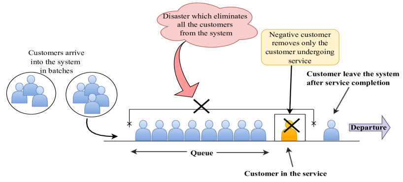
Figure 1: Pictorial representation of the $GI^{X}/M/1$ queue with negative customer and disaster

We consider an infinite buffer queueing model wherein customers (positive customers) arrive into the system in batches and joins the queue. The arriving batch size is a random variable $X$ with probability mass function $P(X=i)=g_{i}$, $i=1,2,\ldots$. For theoretical analysis and numerical implementation we assume that the maximum permissible size of the arriving batch is $b$, which also holds true in many real-world circumstances. Consequently, the mean arriving batch size is $\overline{g}=\sum_{i=1}^{b}ig_{i}$ and the probability generating function is $G(z)=\sum_{i=1}^{b}g_{i}z^{i}$. The inter-arrival times $T$ between the batches are independent and identically distributed continuous random variables with probability density function (pdf) $a(t)$, distribution function $A(t)$, the Laplace-Stieltjes transform (L.S.T) $A^{*}(s)$ and the mean inter-arrival time $\lambda^{-1}=a=-A^{*(1)}(0)$, where $\lambda$ is the arrival rate of the batches and $A^{*(1)}(0)$ is the derivative of $A^{*}(s)$ evaluated at $s=0$. The customers are served individually by a single server and the service time follows exponential distribution with parameter $\mu$.

The system is affected by negative arrivals which is characterized by two independent Poisson arrival processes namely, negative customers and disasters with rate $\eta$ and $\delta$, respectively. The negative customer follows RCH killing discipline and removes only the customer undergoing service, while the occurrence of a disaster eliminates all the customers from the system. We further assume that the negative customer or disaster have no impact on the system when it is empty. The arrival process, service process and the negative arrivals are independent of each other. The model described above may be mathematically denoted by $GI^{X}/M/1$ queue with negative customers and disasters. One may refer to Figure 1 for a pictorial representation of the model.

3 The steady-state analysis

In this section we analyze the model described in Section 2 in steady-state. We first formulate the governing equations of the system using supplementary variable technique (SVT) by considering the remaining inter-arrival time of the next batch as the supplementary variable. For this purpose, we denote the states of the system $N(t)$ and $U(t)$ respectively, as the number of customers in the system and the remaining inter-arrival time of the next batch, at time $t$. We further define

$$q_{n}(u,t)du=P[N(t)=n,u<U(t)\leq u+du],\leavevmode\nobreak\ \leavevmode\nobreak\ n\geq 0,u\geq 0,$$

and in steady-state

$$p_{n}(u)=\lim_{t\rightarrow\infty}q_{n}(u,t).$$

Relating the states of the system at two consecutive epochs $t$ and $t+\Delta t$ and using the arguments of SVT we obtain the following difference-differential equations in steady state.

$$-\frac{d}{du}p_{0}(u) = (\mu+\eta)p_{1}(u)+\delta\sum_{k=1}^{\infty}p_{k}(u),$$ (1)

$$-\frac{d}{du}p_{n}(u) = -(\mu+\eta+\delta)p_{n}(u)+a(u)\sum_{i=1}^{min\{n,b\}}g_{i}p_{n-i}(0)+(\mu+\eta)p_{n+1}(u),\leavevmode\nobreak\ \leavevmode\nobreak\ n\geq 1.$$ (2)

Obtaining the steady-state solution directly from (1) and (2) is a rather difficult task. Therefore, for further analysis we take the transform for which we define

$$p_{n}^{*}(s)=\int_{0}^{\infty}e^{-su}p_{n}(u)du\leavevmode\nobreak\ \Rightarrow\leavevmode\nobreak\ p_{n}=p_{n}^{*}(0)=\int_{0}^{\infty}p_{n}(u)du,\leavevmode\nobreak\ n\geq 0.$$

Multiplying (1)-(2) by $e^{-su}$, integrating with respect to $u$ over $0$ to $\infty$ and then separating equation (2) we obtain the transformed equations as

$$-sp^{*}_{0}(s) = (\mu+\eta)p^{*}_{1}(s)+\delta\sum_{k=1}^{\infty}p_{k}^{*}(s)-p_{0}(0),$$ (3)

$$(\mu+\eta+\delta-s)p^{*}_{n}(s) = A^{*}(s)\sum_{i=1}^{n}g_{i}p_{n-i}(0)+(\mu+\eta)p^{*}_{n+1}(s)-p_{n}(0),\leavevmode\nobreak\ 1\leq n\leq b-1,$$ (4)

$$(\mu+\eta+\delta-s)p^{*}_{n}(s) = A^{*}(s)\sum_{i=1}^{b}g_{i}p_{n-i}(0)+(\mu+\eta)p^{*}_{n+1}(s)-p_{n}(0),\leavevmode\nobreak\ \leavevmode\nobreak\ n\geq b.$$ (5)

Adding (3)-(5) for all values of $n$, taking limit $s\rightarrow 1$ and using the normalizing condition $\sum_{n=0}^{\infty}p_{n}=1$ we have

$$\sum\limits_{n=0}^{\infty}p_{n}(0)=\frac{1}{a}=\lambda.$$ (6)

The L.H.S of equation (6) denotes the mean number of arriving batch into the system per unit time such that the remaining inter-arrival time is 0, which is actually the arrival rate $\lambda$. We now define $p_{n}^{-}$ as the probability that the number of positive customers in the system is $n$ just before the arrival of a batch, i.e., at pre-arrival epoch. Since $p_{n}^{-}$ is proportional to $p_{n}(0)$ and $\sum_{n=0}^{\infty}p_{n}^{-}=1$, we have the relation between $p_{n}^{-}$ and $p_{n}(0)$ as

$$p_{n}^{-}=\frac{p_{n}(0)}{\sum_{k=0}^{\infty}p_{k}(0)}=\frac{p_{n}(0)}{\lambda},\leavevmode\nobreak\ \leavevmode\nobreak\ n\geq 0.$$ (7)

Based on the theory of difference equations we obtain the state probabilities at pre-arrival ($p_{n}^{-}$) and arbitrary ($p_{n}$) epochs in the following section.

3.1 Steady-state system-content distributions

We define the right shift operator $D$ on the sequence of probabilities $\{p_{n}(0)\}$ and $\{p_{n}^{*}(s)\}$ as $Dp_{n}(0)=p_{n+1}(0)$ and $Dp_{n}^{*}(s)=p_{n+1}^{*}(s)$ for all $n$. Thus, (5) can be rewritten in the form

$$\left(\delta-s+(\mu+\eta)(1-D)\right)p^{*}_{n}(s) = \left(A^{*}(s)\sum_{i=1}^{b}g_{i}D^{b-i}-D^{b}\right)p_{n-b}(0),\leavevmode\nobreak\ \leavevmode\nobreak\ n\geq b.$$ (8)

Substituting $s=\delta+(\mu+\eta)(1-D)$ in (8), we get the following homogeneous difference equation with constant coefficient:

$$\left[A^{*}(\delta+(\mu+\eta)(1-D))\sum_{i=1}^{b}g_{i}D^{b-i}-D^{b}\right]p_{n}(0)=0,\leavevmode\nobreak\ \leavevmode\nobreak\ n\geq 0.$$ (9)

The corresponding characteristic equation (c.e.) is

$$A^{*}(\delta+(\mu+\eta)(1-z))\sum_{i=1}^{b}g_{i}z^{b-i}-z^{b}=0,$$ (10)

which has exactly $b$ roots, denoted by $r_{1},r_{2},...,r_{b}$, inside the unit circle $|z|=1$. Thus the solution of (9) is of the form

$$p_{n}(0)=\sum_{i=1}^{b}c_{i}r_{i}^{n},\leavevmode\nobreak\ \leavevmode\nobreak\ n\geq 0,$$ (11)

where $c_{1},c_{2},...,c_{b}$ are the corresponding $b$ arbitrary constants independent of $n$. Now using (11) in (8) we have the following non-homogeneous difference equation

$$(\delta-s+(\mu+\eta)(1-D))p^{*}_{n}(s) = \sum_{j=1}^{b}c_{j}\left(A^{*}(s)\sum_{i=1}^{b}g_{i}r_{j}^{-i}-1\right)r_{j}^{n},\leavevmode\nobreak\ \leavevmode\nobreak\ n\geq b.$$ (12)

The general solution of (12) is of the form

$$p_{n}^{*}(s)=B\left(1+\frac{\delta-s}{\mu+\eta}\right)^{n}+\sum_{j=1}^{b}c_{j}\left\{\frac{A^{*}(s)G(r_{j}^{-1})-1}{\delta-s+(\mu+\eta)(1-r_{j})}\right\}r_{j}^{n},\leavevmode\nobreak\ \leavevmode\nobreak\ n\geq b,$$ (13)

where the first term in the R.H.S of (13) is the solution corresponding to the homogeneous equation of (12) for a fixed $s$, such that $B$ is an arbitrary constant. Meanwhile, the second term in the R.H.S. is a particular solution of (12). Taking limit as $s\rightarrow 0$ and summing over $n$ from $b$ to $\infty$ in (13), we have, $\sum_{n=b}^{\infty}p_{n}^{*}(0)=\sum_{n=b}^{\infty}p_{n}\leq 1$. However, $B\sum_{n=b}^{\infty}\left(1+\frac{\delta-s}{\mu+\eta}\right)^{n}$ tends to infinity as $s\rightarrow 0$. Thus to ensure the convergence of the solution we must have $B=0$ and thus (13) reduces to

$$p_{n}^{*}(s)=\sum_{j=1}^{b}c_{j}\left\{\frac{A^{*}(s)G(r_{j}^{-1})-1}{\delta-s+(\mu+\eta)(1-r_{j})}\right\}r_{j}^{n},\leavevmode\nobreak\ \leavevmode\nobreak\ n\geq b.$$ (14)

We now find the conditions under which $p_{n}^{*}(s)$ satisfies (14) for $1\leq n\leq b-1$ as well. Thus substituting the respective values in (4) we obtain

$$\sum_{j=1}^{b}c_{j}\left(\sum\limits_{i=n+1}^{b}g_{i}r_{j}^{n-i}\right)=0,\leavevmode\nobreak\ 1\leq n\leq b-1,$$

which reduces to the following on using the condition $g_{b}\neq 0$,

$$\sum_{j=1}^{b}c_{j}r_{j}^{n-b}=0,\leavevmode\nobreak\ 1\leq n\leq b-1.$$ (15)

Summing over $n$ from $0$ to $\infty$ in (11) and using relation (6) we obtain

$$\lambda=\sum_{i=1}^{b}\frac{c_{i}}{1-r_{i}}.$$ (16)

One may note that (15) and (16) together constitutes a system of $b$ equations in $b$ unknowns which can be solved to obtain the constants $c_{j}$ for $j=1,2,\ldots,b$. Once $c_{j}$’s are obtained, the expression of $p_{n}(0)$ given in (11) becomes completely known and $p_{n}^{*}(s)$ is given by

$$p_{n}^{*}(s)=\sum_{j=1}^{b}c_{j}\left\{\frac{A^{*}(s)G(r_{j}^{-1})-1}{\delta-s+(\mu+\eta)(1-r_{j})}\right\}r_{j}^{n},\leavevmode\nobreak\ \leavevmode\nobreak\ n\geq 1.$$ (17)

Now, using (7) and (17), the steady-state distribution of the number of positive customers in the system at pre-arrival and arbitrary epochs are given by

$$p_{n}^{-} = \frac{1}{\lambda}\sum\limits_{i=1}^{b}c_{i}r_{i}^{n},\leavevmode\nobreak\ \leavevmode\nobreak\ n\geq 0,$$ (18)

$$p_{n} = p_{n}^{*}(0)=\sum_{j=1}^{b}c_{j}\left\{\frac{G(r_{j}^{-1})-1}{\delta+(\mu+\eta)(1-r_{j})}\right\}r_{j}^{n},\leavevmode\nobreak\ n\geq 1,$$ (19)

$$p_{0} = 1-\sum_{n=1}^{\infty}p_{n}=1-\sum_{j=1}^{b}\frac{c_{j}r_{j}}{1-r_{j}}\left\{\frac{G(r_{j}^{-1})-1}{\delta+(\mu+\eta)(1-r_{j})}\right\}.$$ (20)

This completes the analysis of the model under consideration. It may be noted that the results derived so far are mainly expressed in terms of the roots of the c.e. (10) lying inside the unit circle. It can be proved that $\delta>0$ is a sufficient condition for the c.e. to have exactly $b$ roots inside the unit circle (see Appendix), which ensures the stability of the system. Or in other words, due to the occurrence of disasters the system becomes empty and as a result the model under consideration always remains stable.

Once the probability distributions are completely known, different characteristic measures determining the performance of the system can be easily established. For example, the average population size at pre-arrival ($L^{-}$) and arbitrary ($L$) epochs are given by $L^{-}=\sum_{n=1}^{\infty}np_{n}^{-}$ and $L=\sum_{n=1}^{\infty}np_{n}$, respectively. That is,

$$L^{-}=\frac{1}{\lambda}\sum\limits_{i=1}^{b}\frac{c_{i}r_{i}}{(1-r_{i})^{2}},\leavevmode\nobreak\ \leavevmode\nobreak\ L=\sum_{j=1}^{b}\frac{c_{j}r_{j}}{(1-r_{j})^{2}}\left\{\frac{G(r_{j}^{-1})-1}{\delta+(\mu+\eta)(1-r_{j})}\right\}.$$

4 Special cases

In this section we discuss a few special cases of the model by considering some fixed values of the parameters. As a result our model reduces to some well-known classical queueing models with or without negative arrivals.

Case 1:

If $\eta=0$ and $\delta=0$, i.e., negative customer or disaster does not occur or their occurrence have no impact on the system, then our model reduces to the classical $GI^{X}/M/1$ queue. Consequently, the steady-state distributions of the number of customers in the system at pre-arrival and arbitrary epochs can be obtained directly from (18)-(20) by putting $\eta=0$ and $\delta=0$, where $r_{j}$, $j=1,2,\ldots,b$ are the roots of the c.e. $z^{b}-A^{*}(\mu-\mu z)\sum_{i=1}^{b}g_{i}z^{b-i}=0$ lying inside the unit circle, and then the corresponding arbitrary constants $c_{j}$, $j=1,2,\ldots,b$ can be obtained by solving the system of equations (15) and (16). Here it may be noted that $\lambda\overline{g}<\mu$ is the necessary and sufficient condition for the stability of the system. This particular queueing model has been extensively studied in the literature, both analytically and numerically, based on the use of embedded Markov chain technique and roots method (see Chaudhry and Templeton [11], Bri$\grave{e}$re and Chaudhry [9], Easton et al. [14, 15]). However, the present paper provides an alternative procedure for the solution of the model which is theoretically tractable and easy to implement, as compared to the other approaches.

Meanwhile, setting $\eta=0$, $\delta=0$, $g_{1}=1$ and $g_{i}=0$ for $i\geq 2$ will give the steady-state solution for $GI/M/1$ queue. The c.e. will have a single root inside the unit circle (say $r$) under the condition $\lambda<\mu$, and the corresponding arbitrary constant can be obtained from (16) as $c=\lambda(1-r)$. It is followed by the system-content distributions which can be obtained from (18)-(20).

Case 2:

If $\delta=0$, i.e., the disaster does not play any role and the only negative arrivals are the negative customers, then the model reduces to $GI^{X}/M/1$ queue with negative customers. The c.e. $z^{b}-A^{*}((\mu+\eta)-(\mu+\eta)z)\sum_{i=1}^{b}g_{i}z^{b-i}=0$ will have exactly $b$ roots inside the unit circle under the necessary and sufficient condition $\lambda\overline{g}<\mu+\eta$. Equations (15) and (16) can be solved for the arbitrary constants following which, the steady-state distributions of the number of positive customers in the system can be obtained from (18)-(20). As discussed in Case 1, the solution for $GI/M/1$ queue with negative customers (Yang and Chae [30]) can be further derived by assuming $g_{1}=1$ and $g_{i}=0$ for $i\geq 2$.

Case 3:

If $\eta=0$, the system does not get affected by the negative customers and our model reduces to $GI^{X}/M/1$ queue with disaster. Due to the impact of disasters, the system will always remain stable and hence the c.e. will have exactly $b$ roots inside the unit circle under the sufficient condition $\delta>0$. The steady-state distributions can be derived from (18)-(20) after obtaining the constants from (15) and (16). Similarly as before, the solution for $GI/M/1$ queue with disasters (Park et al. [25]) can also be obtained.

5 Numerical Observation

Table 1: Steady-state distribution of the number of positive customers in the system at various epochs for different inter-arrival time distributions

	$GI=M$			$GI=D$
$n$	$p_{n}^{-}$	$p_{n}$	$p_{n+1}^{-}/p_{n}^{-}$	$p_{n}^{-}$	$p_{n}$	$p_{n+1}^{-}/p_{n}^{-}$
0	0.20533567	0.20533567	0.15065676	0.23080160	0.12004016	0.15318913
1	0.03093521	0.03093521	0.91498603	0.03535630	0.03653976	1.12629474
2	0.02830528	0.02830528	1.65427828	0.03982161	0.03420904	1.01859822
3	0.04682481	0.04682481	0.55001705	0.04056222	0.06060381	0.85997718
4	0.02575445	0.02575445	1.23727398	0.03488259	0.02886916	1.20959058
5	0.03186531	0.03186531	1.45536181	0.04219365	0.04113680	0.92958177
6	0.04637555	0.04637555	0.55360053	0.03922244	0.05948070	0.75644328
7	0.02567353	0.02567353	1.05065616	0.02966955	0.03095702	1.07090478
$\vdots$	$\vdots$	$\vdots$	$\vdots$	$\vdots$	$\vdots$	$\vdots$
200	0.00000060	0.00000060	0.94509121	0.00000009	0.00000010	0.93533903
201	0.00000057	0.00000057	0.94509121	0.00000008	0.00000009	0.93533903
202	0.00000054	0.00000054	0.94509121	0.00000008	0.00000009	0.93533903
203	0.00000051	0.00000051	0.94509121	0.00000007	0.00000008	0.93533903
204	0.00000048	0.00000048	0.94509121	0.00000007	0.00000008	0.93533903
205	0.00000045	0.00000045	0.94509121	0.00000006	0.00000007	0.93533903
$\vdots$	$\vdots$	$\vdots$	$\vdots$	$\vdots$	$\vdots$	$\vdots$
sum	1.00000000	1.00000000		1.00000000	1.00000000
Mean	15.04001756	15.04001756		12.39890533	14.40030123

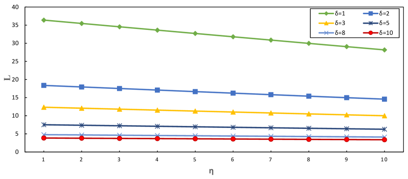
Figure 2: Effect of $\eta$ on $L$ for various $\delta$

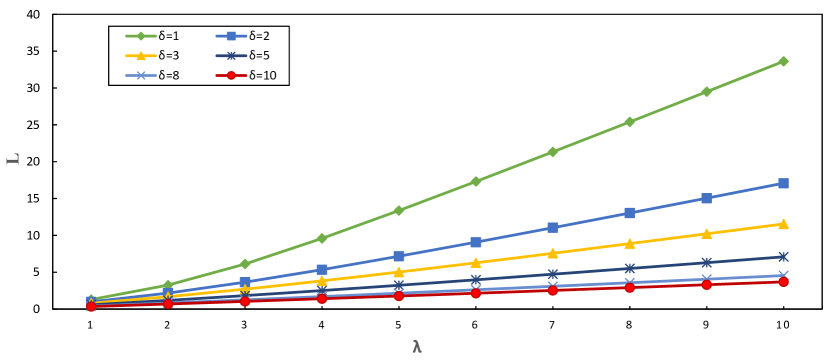
Figure 3: Effect of $\lambda$ on $L$ for various $\delta$

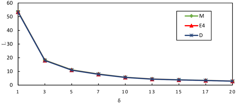
Figure 4: Effect of $\delta$ on $L$ for various interarrival distributions

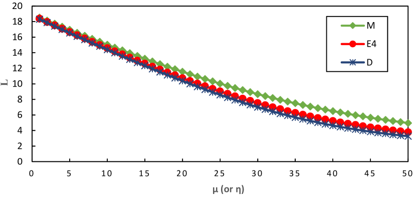
Figure 5: Effect of $\eta$ on $L$ for various interarrival distributions

In this section we demonstrate the analytical results obtained in Section 3 by some numerical examples, which are represented in tabular and graphical form. The results given in the table may be beneficial for other researchers who would like to compare their results using some other methods in the near future.

Table 1 displays the steady-state distribution of the number of positive customers in the system for Poisson ($M$) and deterministic ($D$) arrival processes. The parameters chosen are $\lambda=10$, $\mu=10$, $\eta=5$, $\delta=2$, $g_{1}=0.2$, $g_{3}=0.4$, $g_{6}=0.3$ and $g_{10}=0.1$. The last row of the table depicts the average system content at various epochs. It is important to note that the system-content distributions in the $2^{nd}$ and $3^{rd}$ column are same due to the Poisson arrival process, which verifies the accuracy of our analytical results. Meanwhile, for deterministic inter-arrival time distribution, the L.S.T $A^{*}(s)$ is a transcendental function, which is approximated to a rational function using $Pad\acute{e}(15,15)$ approximation (see Akar and Arikan [2], Singh et al. [26]). Another interesting trend can be observed in the $4^{th}$ and $7^{th}$ column of the table. As $n$ becomes larger, the ratio of the system content distribution at pre-arrival epoch converges to a particular value which is the largest real root (say $r_{b}$) of the c.e. (10) lying inside the unit circle. This suggests that the limiting distributions at the pre-arrival epoch can be approximated by the unique largest root of the c.e. as $p_{n}^{-}=\frac{1}{\lambda}c_{b}r_{b}^{n}$.

Figure 3 investigates the influence of $\eta$ on $L$ for different values of $\delta$. As $\eta$ increase, $L$ decreases for any value of $\delta$, which is intuitive. Similarly, for a fixed $\eta$, $L$ decreases with increasing $\delta$. However, as $\delta$ becomes too large ($\delta=10$), $L$ seems to attain a constant value irrespective of the values of $\eta$. A similar behavior can be experienced on plotting $L$ against $\mu$ for different values of $\delta$, and consequently it is omitted. Figure 3 depicts the impact of $\lambda$ on $L$ for different $\delta$. Clearly, as $\lambda$ increases $L$ increases for any $\delta$. However, when $\lambda$ is kept fixed along with other parameters, $L$ decreases significantly with the increase in $\delta$.

Finally, in Figure 5 and 5 we respectively illustrate the impact of $\delta$ and $\eta$ on $L$ for different inter-arrival time distributions, namely, exponential ($M$), Erlang ($E_{4}$) and deterministic ($D$). It may be observed in Figure 5 that for each inter-arrival time distribution, $L$ decreases as $\delta$ increases, which is obvious. However, for a fixed $\delta$, $L$ is equal for all the three distributions. A possible explanation for this phenomenon may be the frequent occurrence of disasters which removes all the customers including the batch which has just arrived. The effect of inter-arrival time distribution can be best understood from Figure 5 as $\eta$ increases. For higher values of $\eta$, $L$ decreases significantly. However, for exponential inter-arrival time distribution $L$ is greater, and decreases for Erlang followed by deterministic distribution. It may be mentioned that in all the numerical results generated throughout this section, the values of the parameters involved are not restricted to any condition except that $\delta>0$, as the system with disaster is always stable.

6 Concluding remarks

In this paper, the steady-state analysis of a $GI^{X}/M/1$ queueing model with negative customers and disasters has been presented. We have derived the explicit closed-form expressions of the distribution of the number of positive customers in the system at pre-arrival and arbitrary epochs, in terms of roots of the associated characteristic equation. The results of some classical queueing models with or without negative arrivals have been discussed along with their stability conditions. Additionally, through some numerical examples, we have investigated the influence of negative customers and disasters on the performance characteristic of the system. The methodology used in this paper is based on supplementary variable technique and difference equation method which makes the analysis easily tractable, both theoretically and computationally. The procedure developed throughout the analysis can be utilized and further extended to study some more complicated models.

7 Appendix

Theorem 1.

The c.e. $A^{*}(\delta+(\mu+\eta)(1-z))\sum_{i=1}^{b}g_{i}z^{b-i}-z^{b}=0$ have exactly $b$ roots inside the unit circle $|z|=1$ subject to the condition $\delta>0$.

Proof.

Let us assume $f_{1}(z)=-z^{b}$ and $f_{2}(z)=A^{*}(\delta+(\mu+\eta)(1-z))\sum_{i=1}^{b}g_{i}z^{b-i}=K(z)$. Since $A^{*}(\delta+(\mu+\eta)(1-z))\sum_{i=1}^{b}g_{i}z^{b-i}$ is an analytic function, it can be written in the form $K(z)=\sum_{i=1}^{\infty}k_{i}z^{i}$ such that $k_{i}\geq 0$ for all $i$. Consider the circle $|z|=1-\epsilon$ where $\epsilon>0$ and is a sufficiently small quantity. Now

$$|f_{1}(z)| = |z^{b}|=(1-\epsilon)^{b}=1-b\epsilon+o(\epsilon)$$

$$|f_{2}(z)| = |K(z)||\sum_{i=1}^{b}g_{i}z^{b-i}|\leq K(|z|)\sum_{i=1}^{b}g_{i}|z|^{b-i}=K(1-\epsilon)\sum_{i=1}^{b}g_{i}(1-\epsilon)^{b-i}$$

$$= A^{*}(\delta)-\epsilon\{2A^{*}(\delta)(b-\overline{g})-(\mu+\eta)A^{*(1)}(\delta)\}+o(\epsilon)$$

$$< 1-b\epsilon+o(\epsilon)$$

under the sufficient condition $\delta>0$. Thus from Rouch$\acute{e}$’s theorem we have exactly the same number of zeroes in $f_{1}(z)$ and $f_{1}(z)+f_{2}(z)$ inside the unit circle, and hence the theorem. ∎

References

- [1] Karim Abbas and Djamil Aïssani. Strong stability of the embedded Markov chain in an queue with negative customers. Applied Mathematical Modelling, 34(10):2806–2812, 2010.
- [2] Nail Akar and Erdal Arikan. A numerically efficient method for the queue via rational approximations. Queueing systems, 22(1):97–120, 1996.
- [3] Jesus R Artalejo. G-networks: A versatile approach for work removal in queueing networks. European Journal of Operational Research, 126(2):233–249, 2000.
- [4] Ivan Atencia and Pilar Moreno. The discrete-time queue with negative customers and disasters. Computers & Operations Research, 31(9):1537–1548, 2004.
- [5] FP Barbhuiya and UC Gupta. A difference equation approach for analysing a batch service queue with the batch renewal arrival process. Journal of Difference Equations and Applications, pages 1–10, 2019.
- [6] FP Barbhuiya and UC Gupta. Discrete-time queue with batch renewal input and random serving capacity rule: . Queueing Systems, pages 1–19, 2019.
- [7] FP Barbhuiya, Nitin Kumar, and UC Gupta. Batch renewal arrival process subject to geometric catastrophes. Methodology and Computing in Applied Probability, 21(1):69–83, 2019.
- [8] Onno J Boxma, David Perry, and Wolfgang Stadje. Clearing models for queues. Queueing Systems, 38(3):287–306, 2001.
- [9] G Brière and Mohan L Chaudhry. Computational analysis of single-server bulk-arrival queues: . Queueing Systems, 2(2):173–185, 1987.
- [10] SR Chakravarthy. A catastrophic queueing model with delayed action. Applied Mathematical Modelling, 46:631–649, 2017.
- [11] ML Chaudhry and James GC Templeton. First course in bulk queues. John Wiley & Sons, New York, 1983.
- [12] Anyue Chen and Eric Renshaw. The queue with mass exodus and mass arrivals when empty. Journal of Applied Probability, 34(1):192–207, 1997.
- [13] S Dharmaraja and Rakesh Kumar. Transient solution of a Markovian queuing model with heterogeneous servers and catastrophes. Opsearch, 52(4):810–826, 2015.
- [14] Glen Easton, ML Chaudhry, and MJM Posner. Some corrected results for the queue . European journal of operational research, 18(1):131–132, 1984.
- [15] Glen Easton, ML Chaudhry, and MJM Posner. Some numerical results for the queuing system . European journal of operational research, 18(1):133–135, 1984.
- [16] Erol Gelenbe. Random neural networks with negative and positive signals and product form solution. Neural computation, 1(4):502–510, 1989.
- [17] Veena Goswami and GB Mund. Analysis of discrete-time batch service renewal input queue with multiple working vacations. Computers & Industrial Engineering, 61(3):629–636, 2011.
- [18] Peter G Harrison and Edwige Pitel. Sojourn times in single-server queues by negative customers. Journal of Applied Probability, 30(4):943–963, 1993.
- [19] Peter G Harrison and Edwige Pitel. queues with negative arrival: an iteration to solve a fredholm integral equation of the first kind. In MASCOTS’95. Proceedings of the Third International Workshop on Modeling, Analysis, and Simulation of Computer and Telecommunication Systems, pages 423–426. IEEE, 1995.
- [20] Peter G Harrison and Edwige Pitel. The queue with negative customers. Advances in Applied Probability, 28(2):540–566, 1996.
- [21] Gautam Jain and Karl Sigman. A Pollaczek–Khintchine formula for queues with disasters. Journal of Applied Probability, 33(4):1191–1200, 1996.
- [22] Achyutha Krishnamoorthy, Padinhare K Pramod, and Srinivas R Chakravarthy. Queues with interruptions: a survey. Top, 22(1):290–320, 2014.
- [23] B Krishna Kumar and D Arivudainambi. Transient solution of an queue with catastrophes. Computers & Mathematics with applications, 40(10-11):1233–1240, 2000.
- [24] B Krishna Kumar and S Pavai Madheswari. Transient behaviour of the queue with catastrophes. Statistica, 62(1):129–136, 2002.
- [25] Hyun Min Park, Won Seok Yang, and Kyung Chul Chae. Analysis of the queue with disasters. Stochastic analysis and applications, 28(1):44–53, 2009.
- [26] Gagandeep Singh, U C Gupta, and Mohan L Chaudhry. Analysis of queueing-time distributions for queue. International Journal of Computer Mathematics, 91:1911–1930, 2014.
- [27] Don Towsley and Satish K Tripathi. A single server priority queue with server failures and queue flushing. Operations Research Letters, 10(6):353–362, 1991.
- [28] Tien Van Do. Bibliography on G-networks, negative customers and applications. Mathematical and Computer Modelling, 53(1-2):205–212, 2011.
- [29] Jinting Wang, Yunbo Huang, and Zhangmin Dai. A discrete-time on–off source queueing system with negative customers. Computers & Industrial Engineering, 61(4):1226–1232, 2011.
- [30] Won S Yang and Kyung C Chae. A note on the queue with Poisson negative arrivals. Journal of Applied Probability, 38(4):1081–1085, 2001.
- [31] Wen-Hui Zhou. Performance analysis of discrete-time queue with negative arrivals. Applied mathematics and computation, 170(2):1349–1355, 2005.