Sensitivity of the lower-edge of the pair instability black hole mass gap to the treatment of time dependent convection

Abstract

Gravitational-wave detections are now probing the black hole (BH) mass distribution, including the predicted pair-instability mass gap. These data require robust quantitative predictions, which are challenging to obtain. The most massive BH progenitors experience episodic mass ejections on timescales shorter than the convective turn-over timescale. This invalidates the steady-state assumption on which the classic mixing-length theory relies. We compare the final BH masses computed with two different versions of the stellar evolutionary code MESA: (i) using the default implementation of Paxton et al. (2018) and (ii) solving an additional equation accounting for the timescale for convective deceleration. In the second grid, where stronger convection develops during the pulses and carries part of the energy, we find weaker pulses. This leads to lower amounts of mass being ejected and thus higher final BH masses of up to $\sim$ $5\,M_{\odot}$. The differences are much smaller for the progenitors which determine the maximum mass of BHs below the gap. This prediction is robust at $M_{\rm BH,max}\simeq 48\,M_{\odot}$, at least within the idealized context of this study. This is an encouraging indication that current models are robust enough for comparison with the present-day gravitational-wave detections. However, the large differences between individual models emphasize the importance of improving the treatment of convection in stellar models, especially in the light of the data anticipated from the third generation of gravitational wave detectors.

1 Introduction

One of the most challenging aspects of simulating the interior evolution of stars is the treatment of convection (e.g., Renzini, 1987; Arnett et al., 2018a; Buldgen, 2019). The development of convective motion in highly stratified media is an inherently multidimensional problem, which involves turbulence. Spherically symmetric stellar models typically rely on the Mixing Length Theory (MLT, Böhm-Vitense 1958), which provides an averaged description of subsonic, steady-state convection. Albeit with many well-known caveats, MLT is often a sufficient description for the energy transport and chemical mixing provided by convection. This is because the evolutionary timescale of a star is typically much longer than the convective turnover timescale: within a single timestep it is reasonable to assume that the steady state described by MLT can be achieved in the convective layers.

However, some stars can experience dynamical phases of evolution which are too short for convection to achieve the steady state described by MLT. One relevant example is the calculation of the spectrum of asteroseismological pulsations for stars with convective envelopes (e.g., Unno, 1967; Gough, 1977). Cases where the short evolutionary timescale might influence the stellar structure include the helium flash (e.g., Nomoto & Sugimoto, 1977) and more generally any explosive thermonuclear ignition that can drive convection (e.g., Nomoto et al., 1984; Nomoto, 1987; Takahashi et al., 2013), very late evolutionary phases of massive star evolution (e.g., Couch et al., 2015; Chatzopoulos et al., 2016), dynamically unstable mass transfer from a convective donor star (e.g., Paczyński & Sienkiewicz, 1972; Lauterborn & Weigert, 1972), and stellar explosions(e.g., Couch & Ott, 2013). In these situations, the time-dependence of convection can become important, and stellar evolution calculations typically lack a first principles model for the convective acceleration. Sometimes, the convective acceleration due to buoyancy is limited to a fraction of the local gravitational acceleration to prevent unphysically large accelerations (e.g., Arnett, 1969; Wood, 1974).

Here, we focus on a timely example of a situation in which the time dependence of convection can be important: the evolution of very massive stars experiencing pulsational pair instability (PPI, Fowler & Hoyle 1964;Barkat et al. 1967). Because of the large mass required to encounter this instability, it is expected to be a rare phenomenon in nature, but the recent detection of black holes (BH) with masses $30\,M_{\odot}\lesssim M_{\mathrm{BH}}\lesssim 50\,M_{\odot}$ (Abbott et al., 2019a) has driven the interest in understanding the evolution of the most massive (stellar) BH progenitors. To fully harvest the information carried by gravitational waves and use it to constrain stellar evolution, we need to have robust stellar models and characterize their sensitivity to uncertain ingredients (e.g., Farmer et al., 2016; Renzo et al., 2017; Davis et al., 2019; Farmer et al., 2019).

Stars that develop helium (He) core masses exceeding $M_{\mathrm{He}}\gtrsim 30\,M_{\odot}$ are predicted to encounter the PPI and shed significant amounts of mass in subsequent pulsation episodes (e.g., Rakavy & Shaviv, 1967; Yoshida et al., 2016; Woosley, 2017; Takahashi, 2018; Marchant et al., 2019; Leung et al., 2019; Woosley, 2019). The amount of mass lost in these pulses, together with the previous wind mass loss, determines the mass distribution of BHs formed. Increasing further to $M_{\mathrm{He}}\gtrsim 60\,M_{\odot}$, the instability becomes so violent that the entire star is disrupted in a pair-instability supernova (PISN, Barkat et al., 1967; Fraley, 1968), without leaving any compact remnant. For $M_{\mathrm{He}}\gtrsim 135\,M_{\odot}$, all the energy released by the thermonuclear explosion is used to photodisintegrate the newly formed nuclei, instead of accelerating the stellar gas, and BH formation resumes (e.g., Bond et al., 1984). Thus, PISNe are expected to carve a gap in the BH mass distribution.

Numerical simulations of the PPI evolution require following hydrodynamical phases in between phases of hydrostatic equilibrium. This can be done alternating the use of two different codes (e.g., Chatzopoulos & Wheeler, 2012; Chatzopoulos et al., 2013; Yoshida et al., 2016; Takahashi, 2018), which however limits the number of pulsational events that can be followed. To the best of our knowledge, two hydrodynamic Lagrangian stellar evolution codes can now follow the evolution of such massive stars. Woosley (2017, 2019) presented the first grids of stellar models computed with the KEPLER code (Weaver et al., 1978), building upon pre-existing models computed with the same code (Woosley et al., 2002, 2007). Recently, Marchant et al. (2019); Farmer et al. (2019); Renzo et al. (2020) and Leung et al. (2019) used two different implementations of hydrodynamics in the open-source code MESA (Paxton et al., 2011; Paxton et al., 2013, 2015, 2018, 2019) to simulate the evolution of PPI.

Several authors have noted that the amount of mass lost is sensitive to the treatment of convection, both before and during the pulses (e.g., Woosley, 2017; Marchant et al., 2019; Leung et al., 2019). Here, we compare two grids of massive bare He core models to highlight the differences resulting from variations in the treatment of time-dependent convection. In one of our grids, convection is treated similarly to Paxton et al. 2018 and Leung et al. (2019), while the other grid follows the approach used in Marchant et al. (2019) (hereafter, M19) and Farmer et al. (2019). In Sec. 3.1, we present the BH masses from both grids. In Sec. 3.2, we illustrate the differences in internal structure using two pairs of example stellar models. Sec. 4 compares the two treatments of time-dependent convection adopted here to other implementations existing in the literature and summarizes the main limitations of this study. We discuss the implications of our results in Sec. 5.

We do not aim at solving a problem that has remained in stellar astrophysics for several decades, but hope to stimulate improvements in stellar evolution models that also account for the time-dependent behavior of convective motion.

2 Methods

We use the open-source stellar evolution code MESA to simulate the evolution of bare He cores at metallicity $Z=0.001$ with masses in the range $25\,M_{\odot}\leq M_{\mathrm{He}}\leq 70\,M_{\odot}$. All our input files are available at http://cococubed.asu.edu/mesa_market/inlists.html, and our models are available at doi:10.5281/zenodo.3406320. We track the energy generation with the 22-isotope nuclear reaction network approx21_plus_co56.net. Slightly before the star becomes dynamically unstable, i.e., the pressure weighted volumetric averaged adiabatic index approaches 4/3 (e.g., Stothers, 1999)

$$\langle\Gamma_{1}\rangle\stackrel{{\scriptstyle\mathrm{def}}}{{=}}\frac{\int\Gamma_{1}P\,d^{3}r}{\int P\,d^{3}r}\equiv\frac{\int\Gamma_{1}\frac{P}{\rho}\,dm}{\int\frac{P}{\rho}\,dm}\lesssim\frac{4}{3}\ \ ,$$ (1)

we employ the HLLC Riemann solver in MESA (Toro et al., 1994), without relying on artificial viscosity to capture shocks. After a dynamical pulse, if/once the core has recovered hydrostatic equilibrium, we create a new stellar model of reduced mass with the entropy and chemical profile of the bound material. We do not include any wind mass loss, although the treatment of winds is known to influence the core structure of massive stars (Renzo et al., 2017). Preliminary tests including wind mass loss showed the same trends discussed here. The impact of uncertainties related to winds and other input physics on our PPI models are studied in Farmer et al. (2019). Tests to ensure the robustness of our models against spatial and temporal discretization are discussed in (M19, Farmer et al. 2019, Renzo et al. 2020). We refer the interested readers to M19 for a full description of our setup. Here, we focus only on the treatment of convection.

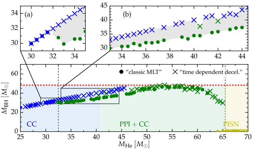
Figure 1: BH mass as a function of the He core mass for our two grids. The color shading indicates the approximate boundaries between evolution to core-collapse (CC, blue), pulsational pair-instability mass loss $\gtrsim 3\,M_{\odot}$ (PPI+CC, green), and full disruption in a PISN (yellow). The gray area in the inset panels shows the systematic offset we find in the final BH masses from our two grids. The dashed red line indicates the maximum BH mass we find below the PISN BH mass gap (white area in the bottom panel), which is not sensitive to the variations between our two grids of models.

We adopt the Ledoux criterion for convective stability with a mixing length parameter $\alpha_{\rm MLT}=2.0$ and an exponential under/overshooting with (f,f_0) = (0.01,0.005) (cf. Eq. 2 in Paxton et al., 2011). To test the sensitivity of our results to the treatment of time-dependent convection, we compute two grids of models using two different MESA versions. Other differences between the two code versions might contribute to the variations described here. Our first grid of models, which we refer to as the “classic MLT” grid, is computed using MESA release 10108. For this grid, the convective velocity $v_{c}$ is obtained from MLT under the steady-state assumption, similarly to Paxton et al. (2018) and Leung et al. (2019), although the latter authors turn off convection during hydrodynamical phases of evolution. For this grid we employ MLT++, which is an enhancement of the convective flux in superadiabatic radiation-pressure dominated regions prone to developing density inversions (Paxton et al., 2013; Jiang et al., 2018) and a semiconvection efficiency of 0.01. We do not employ thermohaline mixing for numerical stability reasons. After the onset of the hydrodynamic phase of evolution we enforce short timesteps, therefore we apply a limit to the convective acceleration based on Wood (1974) to avoid unphysical infinite convective acceleration. This approach still allows for infinite convective deceleration: if a stellar layer becomes radiatively stable, the convective velocity is instantaneously set to zero.

We compute our second grid, which we refer to as the “time dependent deceleration” grid, using MESA version 11123. In this case, we obtain $v_{c}$ solving, together with the stellar structure and composition equations, an equation designed to asymptotically give the MLT value of $v_{c}$ over long timescales, and to damp $v_{c}$ in radiative regions over a characteristic buoyancy timescale. The equation we solve reads (cf. Eq. A1 and A2 in M19 and Eq. 11 in Arnett 1969):

$$\frac{\partial v_{c}}{\partial t}=\begin{cases}(v_{\rm MLT}^{2}-v_{c}^{2})/\lambda&\quad\rm{for\ convectively\ unstable\ regions}\quad,\\ -v_{c}^{2}/\lambda-Nv_{c}&\quad\rm{for\ convectively\ stable\ regions}\qquad,\end{cases}$$ (2)

where $\lambda=\alpha_{\rm MLT}H_{p}$ is the mixing length, assumed to be proportional through a free parameter $\alpha_{\mathrm{MLT}}$ to the local pressure scale height $H_{p}$, $N$ is the Brunt-Väisälä frequency, and $v_{\mathrm{MLT}}$ is the MLT steady state convective velocity. In this second “time dependent deceleration” grid, we do not employ MLT++. Semiconvection and thermohaline mixing are treated in the same way as in our “classic MLT” grid.

These two implementations of time dependent convection do not exhaust all the possible choices (e.g., Unno, 1967, see also Sec. 4.1), but are sufficient to illustrate the qualitative and quantitative differences that can be expected in computing the evolution through PPI.

Our main parameter of interest is the resulting BH mass, which we estimate using the mass coordinate where the gravitational binding energy reaches $10^{48}\,\mathrm{ergs}$. This allows for the possibility of mass loss during the final core-collapse from either a weak explosion (Ott et al., 2018; Kuroda et al., 2018), energy loss to neutrinos, or ejection of a fraction of the envelope caused by the latter (e.g., Nadezhin, 1980; Lovegrove & Woosley, 2013). This typically gives estimated BH masses within a few $0.01\,M_{\odot}$ of the total baryonic mass slower than the escape velocity at the onset of core collapse.

3 Results

3.1 Impact on the BH masses

Figure 1 shows the BH masses resulting from our numerical experiment. Dots show models from our “classic MLT” grid, where increases in $v_{c}$ are limited following Wood (1974) and the decreases in $v_{c}$ are unlimited, while crosses mark the BH masses for models in our “time dependent deceleration” grid, which uses Eq. 2. The two inset panels emphasize the main differences found, which could affect both the the BH mass function and their detection rate in gravitational-wave events.

The colors in Fig. 1 emphasize in blue the range of $M_{\mathrm{He}}$ that collapse without any PPI-driven mass ejection (CC) and in green the PPI range, which we define here requiring that PPI remove at least $3\,M_{\odot}$. The yellow region shows models fully disrupted in a PISN. The boundary mass between PPI+CC behavior and full disruption only shifts by $\sim$ $3\,M_{\odot}$ between our two grids. This is smaller than variations induced by other uncertainties (e.g., nuclear reaction rates and metallicity, Farmer et al. 2019).

The inset (a) of Fig. 1 magnifies the range at which PPI starts, around $M_{\mathrm{He}}\simeq 32\,M_{\odot}$. This mass threshold for the occurrence of thermonuclear explosions driven by the pair instability is in very good agreement with Woosley (2017, 2019). The models from our “time dependent convective deceleration” grid (crosses) show, in this mass range, a one-to-one linear correspondence between $M_{\mathrm{He}}$ and the BH mass. The occurrence of weak pulses does not drive significant mass loss, blurring the boundary between CC and PPI+CC evolution. Instead, the approach used in our “classic MLT” grid produces stronger pulses at the low mass end, resulting in a turn-over in $M_{\mathrm{BH}}\equiv M_{\mathrm{BH}}(M_{\mathrm{He}})$. Since lower mass He cores are expected to be more common, if the pulses of the least massive stars experiencing PPI can remove a significant amount of mass, then it might be possible to detect an overabundance of BHs of mass corresponding roughly to the minimum $M_{\mathrm{He}}$ for PPI.

The different amount of PPI mass loss for $M_{\mathrm{He}}\lesssim 45\,M_{\odot}$ results in a systematic offset in the final BH masses of $\sim$ $5\,M_{\odot}$, shown in the inset (b) of Fig. 1, and highlighted by the gray background in both inset panels. Models in the “time dependent convective deceleration” grid generally produce more massive BHs, i.e., weaker pulses. This offset might affect the mass-dependent binary BH merger rate by changing which stars make BHs of a given mass. At $M_{\mathrm{He}}\simeq 45\,M_{\odot}$, the “time dependent deceleration” grid shows hints of a turn-over qualitatively similar to the one at 32$\,M_{\odot}$ for our “classic MLT” grid, cf. inset (a). This feature might produce a concentration of BHs at the corresponding BH mass $M_{\mathrm{BH}}\simeq 43\,M_{\odot}$.

The PISN BH mass gap (the first part of which is shown by the white region in Fig. 1) starts above $M_{\mathrm{BH}}\simeq 48\,M_{\odot}$ for both our grids, also in agreement with Woosley (2017, 2019). The different treatment of time-dependent convection in our two grids does not change the maximum BH mass below the PISN BH mass gap significantly (red dashed line in Fig. 1), corroborating the results of Farmer et al. (2019). For $M_{\mathrm{He}}\gtrsim 45\,M_{\odot}$ the scatter in BH masses increases, owing to the combination of more energetic pulses and the lack of wind mass loss in both our grids. The lack of winds, a situation possibly relevant for zero-metallicity population III stars, produces structures with sharp density drops: these influence the propagation of shocks in the star and the amount of mass they remove. From a computational perspective they result in numerically less stable models. Wind mass loss (indirectly) and multi-dimensional effects are likely to smooth these boundaries in nature.

3.2 Illustrative examples

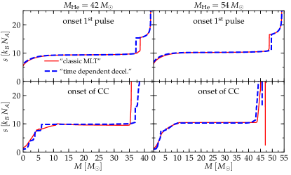
Figure 2: Specific entropy as a function of mass when the average adiabatic index $\langle\Gamma_{1}\rangle$ approaches 4/3 (top row) and at the onset of the final core-collapse (bottom row). Red solid lines are models from our “classic MLT” grid, while thick blue dashed lines are models from our “time dependent deceleration” grid. We show a $42\,M_{\odot}$ model representative of the behavior of in the insets in Fig. 1 (left column) and a $54\,M_{\odot}$ model representative of the progenitors of the most massive BHs below the PISN mass gap (right column).

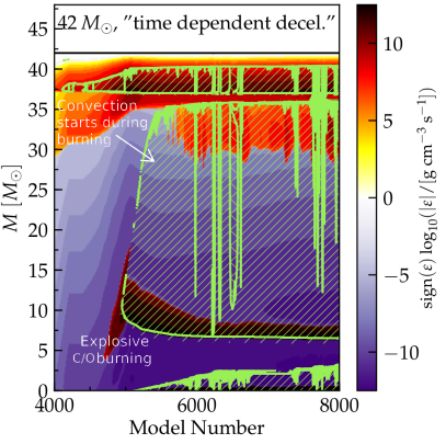
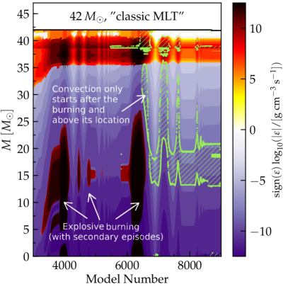
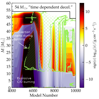
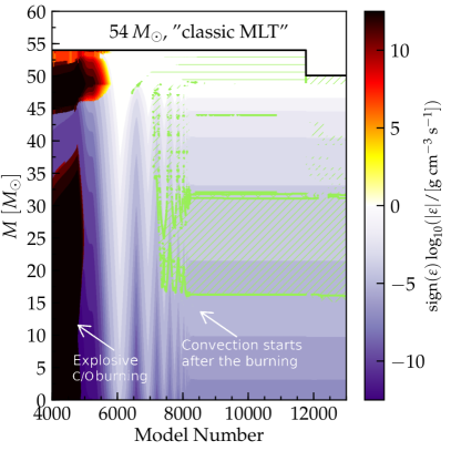
Figure 3: Kippenhahn diagrams during the development and propagation of the first pulse for the $42\,M_{\odot}$ (top row) and $54\,M_{\odot}$ (bottom row) shown in Fig. 2. The left panels show the evolution for our “time dependent deceleration” approach, while the right panels show the corresponding evolution for the “classic MLT”. $\varepsilon=\varepsilon_{\mathrm{nuc}}-\varepsilon_{\nu}$ is the energy generation rate from nuclear burning minus the neutrino losses, there is net energy release for the red and black colors, and net energy loss for purple and blue colors. The green hatching indicates convective layers. The solid black line indicates the total mass of the models. A fraction of it becomes unbound earlier than it is removed from the computational domain.

To illustrate the different internal evolution of the stars in our grids we focus here on two pairs of models, of $42\,M_{\odot}$ and $54\,M_{\odot}$ respectively. The first pair is representative of models in the insets of Fig. 1, the second pair is representative of the progenitors of the most massive BHs below the PISN gap.

Figure 2 shows the specific entropy as a function of mass coordinate for these models in the conventional units of Boltzmann’s constant $k_{B}$ times Avogadro’s number $N_{A}$. The specific entropy characterizes the thermodynamic state of the gas, and it is therefore useful when discussing thermal instabilities such as convection. Flat entropy profiles are a signature of efficient convection.

For these models, the internal evolution is similar until the onset of the first pulse and results in similar pre-pulse entropy profiles (top panels). The behavior of convective shells during the pulses (i.e., when the star evolves on a dynamical timescale) shows a consistent difference in the two grids. This can lead to divergent evolution and different entropy profiles and final BH masses (at the lower mass end), or not be sufficient to cause large differences in the final entropy profile or BH mass (for the more massive PPI progenitors). The insets of Fig. 1, and the $42\,M_{\odot}$ models in left panels of Fig. 2 show examples where the pulses drive significant differences. Conversely, the $54\,M_{\odot}$ models in the right column of Fig. 2 are an example where the differences in the convective acceleration/deceleration are not sufficient to cause a different final BH mass and entropy profile.

Figure 3 shows the Kippenhahn diagrams for the $42\,M_{\odot}$ (top) and $54\,M_{\odot}$ (bottom) example models in our “time dependent deceleration” (left column) and “classic MLT” (right column) grids. These illustrate the differences in convective patterns for our two grids during the pulses.

The age of the stars at the start of the pulses differ by a few thousand years, a difference that we do not consider significant given other numerical differences unrelated to the treatment of convection in our grids. The time range shown is larger by a factor of $\sim$ $30$ in the models from the “time dependent deceleration” (right column), but corresponds to a smaller number of timesteps. This is because we can run with the hydrodynamics on for much longer and take longer timesteps thanks to the improved numerical stability of the “time dependent deceleration” grid (see also Appendix  A).

The oxygen thermonuclear explosion during the first pulse (roughly between model number $\sim$ $3\,000-6\,000$) proceeds differently in our two grids. In the “time dependent deceleration” models (left), the oxygen ignition triggers convective mixing (green hatched areas) during the main burning episode. Convection remains in the intermediate layers of the star until and beyond the ejection of mass. Conversely, in the “classic MLT” models (right panels of Fig. 3) the thermonuclear explosion of oxygen is entirely radiative, and convection turns on only after the main burning episode is over, as the pulse wave propagates outward. As the core readjusts dynamically to the energy released, secondary burning episodes are clearly visible in the $42\,M_{\odot}$ model in the top right of Fig. 3.

We think that the different development of convection occurs because at its onset, computational zones of the models tend to oscillate between radiative stability and convective instability. In the “classic MLT” grid, where infinite convective deceleration is allowed, the convective velocity of such zones is reset to zero each time they oscillate back to radiative stability. Conversely, in the “time dependent deceleration” grid, such zones retain a non-zero convective velocity. The instantaneous value of the energy flux can thus vary between these two approaches, and this creates a numerical degeneracy between the convective deceleration, the onset of convection, and the mixing processes happening at the boundary of the convective regions (including the treatment of undershooting, semiconvection, and thermohaline mixing).

At the lower mass end of the PPI regime (for $M_{\mathrm{He}}\lesssim 45\,M_{\odot}$), in the “time dependent deceleration” grid, the presence of convection during the main burning episode leads to efficient outward transport of energy and until it can eventually be radiated away. Conversely, in the the “classic MLT” grid (left column of Fig. 3), where convection does not develop as promptly, the energy released in the thermonuclear explosion remains trapped in the star. Ultimately, this energy contributes to the kinetic energy of the gas and results in stronger mass ejections, producing the kink in inset (a) of Fig. 1 and the offset in inset (b).

The development of large convective shell during the outward propagation of a pulse in the “time dependent deceleration” grids can lead to the injection of helium into the hotter and deeper regions, and consequently to a large increase in nuclear energy generation rate within the convective region. However the evolutionary timescale is set by the dynamical propagation of the pulse, and it is much shorter than the nuclear timescale. Therefore, while this burning changes the chemical profile inside the star, it does not release an amount of energy sufficient to modify significantly the dynamics of the pulse propagation. Indeed, the amount of mass lost by both our $54\,M_{\odot}$ models (bottom row of Fig. 3) in the first pulse is similar, at about $4\,M_{\odot}$.

The lack of differences at the high mass end happens because the more massive progenitors experience fewer but more energetic pulses (Woosley, 2017; Marchant et al., 2019; Renzo et al., 2020) and these are strong enough to develop and sustain convection regardless of which algorithm is used. The two algorithms we compare differ for how convection develops (and damps), but once convection is going on they yield similar results. In either case, the energy released by the thermonuclear explosion during a pulse exceeds the amount that convection carries away. The remaining differences in the resulting BH masses are smaller than those introduced by other physical uncertainties (e.g., nuclear reaction rates and overshooting, Farmer et al. 2019).

Consequently, the maximum BH mass below the PISN BH mass gap, which is produced by models at the more massive end (cf. Fig. 1), is robustly predicted at $\sim$$48\,M_{\odot}$ for models that do not experience wind mass loss (see also Farmer et al., 2019), and does not depend on the treatment of the convective deceleration, at least within the framework of our comparison.

4 Discussion

4.1 Other time-dependent treatments of convection

The treatment of convection is a computationally challenging aspect of stellar evolution (e.g., Renzini, 1987). The specific aspect we focus on here is its time-dependence, which becomes important when the timescale of interest for the star is comparable to, or shorter than, the convective turnover timescale.

Efforts to include the time dependence of convection in stellar evolution calculations can be divided in two categories: (i) those trying to capture time-dependent perturbations on a pre-existing steady state described by MLT, and (ii) those concerned with the growth (or damping) of the convective instability from the radiative equilibrium (or from the MLT steady state). Examples of (i) are the calculations of the eigen-spectrum of stars with convective envelopes (e.g., Unno 1967, Gough 1977, see also Sec. 2 in Paxton et al. 2019). The algorithm developed by Unno (1967) in this context has also been applied to the problem of the growth of the convective instability (e.g., Nomoto & Sugimoto, 1977; Takahashi et al., 2013). Examples of (ii) are the algorithms of Wood (1974) and Arnett (1969) on which our calculations are based.

The importance of convection in the context of PPI evolution was investigated first by Fraley (1968), and has been underlined in many studies since then (e.g., Woosley, 2017; Leung et al., 2019; Marchant et al., 2019; Farmer et al., 2019). Modern calculations of PPI evolution either turn off convection during the hydrodynamic phase of evolution for numerical stability (e.g., Leung et al., 2019), implement a limit on the convective acceleration based on the local gravitational acceleration, leaving the convective deceleration unlimited (as in our “classic MLT” grid), or use an ad-hoc equation to solve for the convective velocity (see Eq. 2 that we use in our “time dependent deceleration” grid, see also Marchant et al. 2019; Farmer et al. 2019; Renzo et al. 2020). The last two approaches fall into the category (ii) of dealing with how the steady state described by MLT develops, and they differ mainly for the inclusion or lack of a timescale for the damping of convection. Our numerical experiments show that changing the convective deceleration leads in a different onset of the convective instability in our models.

Models based on the first approach (i) implicitly assume for the convective velocity field the MLT value and compute small and time-dependent perturbations to it (see also Gough, 1977). This is in principle not applicable to the case of PPI evolution, where the convective instability grows as the star evolves and the “perturbation” in the velocity is the convective velocity itself. A comparison between these two classes of treatments is beyond the scope of the present study, although it would be interesting given the use of the Unno 1967 algorithm in other cases where the relevant problem is the growth of convection.

4.2 Further caveats

We have carried out several experiments to ensure the numerical convergence with increasing spatial and temporal resolution of our PPI models, as presented in appendix B of Marchant et al. (2019), in Farmer et al. (2019), and appendix A of Renzo et al. (2020). Nevertheless, we cannot exclude that the treatment of convection is numerically degenerate with other minor differences in the two MESA versions we employ here.

Of particular concern is the entrainment of the bottom edge of the He-burning shell. In some of our models, this shell moves downwards in mass coordinate, increasing the entropy of the outer layers of the CO core, i.e., decreasing the total amount of mass at low entropy. We find no clear trends in what determines whether the burning shell penetrates downwards or not: this can happen in models that do not experience PPI mass loss, but also in models that later on undergo pulses. This can lead to differences in the pre-pulse entropy profiles which are not driven by the different treatment of the time dependence of convection, since they develop during evolutionary phases when the star evolves on a much longer timescale than the convective turnover timescale.

We suspect that this behavior depends on the sharp density and composition profiles we obtain in the absence of winds, and differences in the numerical setup in the two MESA versions we employ. We have also found that turning off convective undershooting or increasing the efficiency of semiconvective mixing can also influence this behavior. Models computed with the “time dependent deceleration” setup but no undershooting result in BH masses in between the values shown in Fig. 1.

Nevertheless, regardless of the behavior of the He shell, the development of convection during the dynamical phase of a pulse always resembles what shown in Fig. 3. We expect that the improvements in the treatment of convection are the main reason for the differences, but we caution that we cannot exclude that other minor differences contribute. We hope that cleaner numerical experiments with improved models for the development/damping of convection will become possible.

Finally, we emphasize that our calculations and the resulting BH mass in Fig. 1 do not account for possible consequences of binary interactions, as they are obtained from the evolution of single He cores. Further work to assess how binarity can modify the evolution through PPI is needed to interpret gravitational-wave events assuming the isolated binary evolution scenario.

5 Summary & Conclusion

The ongoing search for gravitational waves is starting to provide direct constraints on the BH mass function and probe the theoretically predicted PISN BH mass gap (Fishbach & Holz, 2017; Abbott et al., 2019b; Stevenson et al., 2019). This offers an unprecedented tool to understand the physics of their massive star progenitors. This requires quantitative predictions from stellar models robust enough for a sensible confrontation with the data. The variations in the model predictions resulting from algorithmic choices or simplifying assumptions should be small compared to the input physics that we wish to test and the observational uncertainties.

We have compared the predictions for the final BH masses at the lower edge of the predicted mass gap computed with two different versions and setups of the stellar evolutionary code MESA, which differ primarily in the treatment of the time dependence of convection. Our “classic MLT” grid adopts the defaults of Paxton et al. (2018), while in our “time dependent deceleration” grid we solve an additional equation incorporating the timescale for the damping of convection. Different groups have recently used setups very similar to the two options we compare here (M19, Leung et al. 2019, Farmer et al. 2019, Renzo et al. 2020).

We find systematic differences when comparing individual models for the same initial mass. The final BH masses computed with our time-dependent treatment of convective deceleration are lower by up to $\sim$ $5\,M_{\odot}$ than those in our grid computed adopting the classic mixing length theory. After inspection of the evolution of the internal structure, this seems to be a consequence of more prompt and stronger convection during the propagation of a pulse. Convection carries out part of the energy, preventing it from becoming bulk kinetic energy of ejecta. This results in weaker pulses and a lower amount of mass ejected. The differences are largest for models near the lower end of the mass range for pair pulsations to occur ($32\,M_{\odot}\lesssim M_{\mathrm{He}}\lesssim 45\,M_{\odot}$), but are less important for the higher mass range ($45\,M_{\odot}\lesssim M_{\mathrm{He}}\lesssim 64\,M_{\odot}$), because in these models convection develops regardless of the algorithm employed, but is never sufficient to remove a large fraction of the energy released in the thermonuclear explosion. Because of this, we find that the predicted maximum BH mass for BHs below the gap is robust at $\sim$ $48\,M_{\odot}$.

For now, the robustness of the prediction for the location of the edge of the gap is encouraging. Even the variations we find between the grids for individual masses are smaller than the typical uncertainties on the individual BH masses inferred from gravitational-wave detections.

For the future, our results should be taken as a warning. The variations we find between individual models are substantial. The constraints from gravitational-wave events will become increasingly precise with more detections. Moreover, we can anticipate an increasing number of events detected with high signal-to-noise ratio, and thus more accurately determined parameters for the individual BHs. This will increase the the robustness needed from the stellar model predictions.

The treatment of convection will likely remain a multifaceted challenge, of which the time-dependence is only one aspect, complimentary to other well known issues, but there are several ways forward. Multi-dimensional hydrodynamic simulations applicable to the stellar regime can be used to derive a more realistic expressions that can be included in stellar evolutionary codes (e.g., Meakin & Arnett, 2007; Couch & Ott, 2013; Couch & O’Connor, 2014; Arnett et al., 2018a, b; Yoshida et al., 2019). As a first step, a physically-motivated expression for the convective acceleration in the right hand side of Eq. 2 could be derived from the flow observed in multi-dimensional hydrodynamic simulations, instead of the ad-hoc parametrizations presently used.

The increasing number of gravitational-wave events detected will provide a major motivation for further improving the progenitor models. The anticipated capabilities of third-generation detectors are particularly promising. These should be able to detect massive binary BHs across all redshifts where significant star formation occured in the Universe. They would enable us to probe the evolution of the BH mass distribution as a function of redshift and uncover possible detailed features in the shape of the mass distribution, which bears the imprints of the physical processes that govern the lives of their massive star progenitors.

Acknowledgements: We thank M. Cantiello, D. Hendriks, E. Laplace, and L. van Son for helpful discussions. MR, SJ, and SdM acknowledge funding by the European Union’s Horizon 2020 research and innovation programme from the European Research Council (ERC), Grant agreement No. 715063), and by the Netherlands Organisation for Scientific Research (NWO) as part of the Vidi research program BinWaves with project number 639.042.728. RF is supported by the Netherlands Organisation for Scientific Research (NWO) through a top module 2 grant with project number 614.001.501 (PI de Mink). This research was supported in part by the National Science Foundation under Grant No. NSF PHY-1748958, and stimulated by discussions at the “The Mysteries and Inner Workings of Massive Stars” at KITP. Simulations were carried out on the Dutch national e-infrastructure (Cartesius, project number 16343) with the support of the SURF Cooperative.

Appendix A Evolutionary timescales post-pulse

To clarify the onset of convection in our MESA models, Fig. 3 shows the Kippenhahn diagrams using a non-physical quantity as x coordinate, namely the model number. Since our models are not computed with a fixed timestep, this makes it hard to read the amount of time elapsed. The total time elapsed corresponds to roughly a few tenths of a year, as shown in Fig. 4.

Fig. 4 shows the evolution of the model number and timestep size $\delta t$ (top two panels), together with some global quantities (the Kelvin-Helmholtz timescale $\tau_{\mathrm{KH}}$ and nuclear luminosity $L_{\mathrm{nuc}}$ integrated throughout the star, third and fourth panels from the top), and the central temperature $T_{c}$ (bottom panel) of the models shown in Fig. 3. These quantitites are shown as a function of the time elapsed since we turn on the HLLC solver (cf. Eq. 1), defined as $\Delta t=0$. As in Fig. 2, solid red curves show the “classic MLT” models, and blue thicker dashed curves show the “time dependent deceleration” models. The left column shows the $42\,M_{\odot}$ models, while the right column shows the $54\,M_{\odot}$ models (corresponding respectively to the top and bottom rows of Fig. 3). We chose the vertical and horizontal ranges to encompass the entire evolution shown in Fig. 3 for all these models.

The Kelvin-Helmholtz timescale shown in the third panel is computed as a function of the total mass and radius of the models, however, these may include a significant amount of matter that is unbound and expanding rapidly to very large radii. At the onset of the pulses, the stars are evolving dynamically, on a much shorter timescale, and might temporarily be out of virial equilibrium because of the changing distribution of mass and consequently moment of inertia.

The spikes in $L_{\mathrm{nuc}}$ in the “classic MLT” $42\,M_{\odot}$ models correspond to the secondary burning episodes highlighted in the top right panel of Fig. 3, and they correlate with a strong decrease in the timestep size and consequent increase of the model number around a given $\Delta t$. The use of Eq. 2 in the “time dependent deceleration models” allows us to use generally longer timesteps, turn on the HLLC earlier (more physical time elapses between $\Delta t=0$ and the first spike in $T_{c}$ corresponding a thermonuclear explosion), and keep it on for a longer physical time.

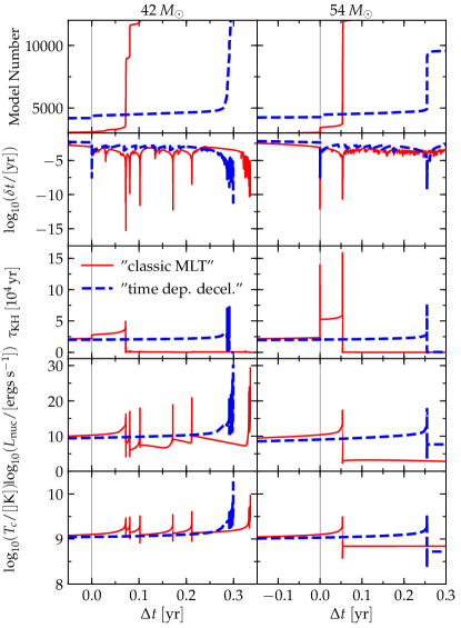
Figure 4: From top to bottom: evolution as a function of time $\Delta t$ since the onset of the dynamical instability (marked by the thin vertical line) of model number, timestep size $\delta t$, Kelvin-Helmholtz timescale, nuclear luminosity, and central temperature. Red solid curve show the “classic MLT” models, while blue dashed curves show the “time dependent deceleration” models. The left (right) column shows the $42\,M_{\odot}$ ($54\,M_{\odot}$) pair of models.

References

- Abbott et al. (2019a) Abbott B. P., Abbott R., Abbott T. D., Abraham S., Acernese F., Ackley K., Adams C., Adhikari R. X., 2019a, Physical Review X, 9, 031040
- Abbott et al. (2019b) Abbott B. P., Abbott R., Abbott T. D., Abraham S., et al. 2019b, ApJ, 882, L24
- Arnett (1969) Arnett W. D., 1969, Ap&SS, 5, 180
- Arnett et al. (2018a) Arnett W. D., Meakin C., Hirschi R., Cristini A., Georgy C., Campbell S., Scott L., Kaiser E., 2018a, arXiv:1810.04653,
- Arnett et al. (2018b) Arnett W. D., Meakin C., Hirschi R., Cristini A., Georgy C., Campbell S., Scott L. J. A., Kaiser E. A., 2018b, arXiv:1810.04659,
- Barkat et al. (1967) Barkat Z., Rakavy G., Sack N., 1967, Phys. Rev. Lett., 18, 379
- Böhm-Vitense (1958) Böhm-Vitense E., 1958, Z. Astrophys., 46, 108
- Bond et al. (1984) Bond J. R., Arnett W. D., Carr B. J., 1984, ApJ, 280, 825
- Buldgen (2019) Buldgen G., 2019, arXiv:1902.10399, p. arXiv:1902.10399
- Chatzopoulos & Wheeler (2012) Chatzopoulos E., Wheeler J. C., 2012, ApJ, 748, 42
- Chatzopoulos et al. (2013) Chatzopoulos E., Wheeler J. C., Couch S. M., 2013, ApJ, 776, 129
- Chatzopoulos et al. (2016) Chatzopoulos E., Couch S. M., Arnett W. D., Timmes F. X., 2016, ApJ, 822, 61
- Couch & O’Connor (2014) Couch S. M., O’Connor E. P., 2014, ApJ, 785, 123
- Couch & Ott (2013) Couch S. M., Ott C. D., 2013, ApJ, 778, L7
- Couch et al. (2015) Couch S. M., Chatzopoulos E., Arnett W. D., Timmes F. X., 2015, ApJ, 808, L21
- Davis et al. (2019) Davis A., Jones S., Herwig F., 2019, MNRAS, 484, 3921
- Farmer et al. (2016) Farmer R., Fields C. E., Petermann I., Dessart L., Cantiello M., Paxton B., Timmes F. X., 2016, ApJS, 227, 22
- Farmer et al. (2019) Farmer R., Renzo M., de Mink S. E., Marchant P., Justham S., 2019, arXiv e-prints, p. arXiv:1910.12874
- Fishbach & Holz (2017) Fishbach M., Holz D. E., 2017, ApJ, 851, L25
- Fowler & Hoyle (1964) Fowler W. A., Hoyle F., 1964, ApJS, 9, 201
- Fraley (1968) Fraley G. S., 1968, Ap&SS, 2, 96
- Gough (1977) Gough D. O., 1977, ApJ, 214, 196
- Jiang et al. (2018) Jiang Y.-F., Cantiello M., Bildsten L., Quataert E., Blaes O., Stone J., 2018, Nature, 561, 498
- Kuroda et al. (2018) Kuroda T., Kotake K., Takiwaki T., Thielemann F.-K., 2018, MNRAS, 477, L80
- Lauterborn & Weigert (1972) Lauterborn D., Weigert A., 1972, A&A, 18, 294
- Leung et al. (2019) Leung S.-C., Nomoto K., Blinnikov S., 2019, arXiv:1901.11136,
- Lovegrove & Woosley (2013) Lovegrove E., Woosley S. E., 2013, ApJ, 769, 109
- Marchant et al. (2019) Marchant P., Renzo M., Farmer R., Pappas K. M. W., Taam R. E., de Mink S. E., Kalogera V., 2019, ApJ, 882, 36
- Meakin & Arnett (2007) Meakin C. A., Arnett D., 2007, ApJ, 667, 448
- Nadezhin (1980) Nadezhin D. K., 1980, Ap&SS, 69, 115
- Nomoto (1987) Nomoto K., 1987, ApJ, 322, 206
- Nomoto & Sugimoto (1977) Nomoto K., Sugimoto D., 1977, PASJ, 29, 765
- Nomoto et al. (1984) Nomoto K., Thielemann F. K., Yokoi K., 1984, ApJ, 286, 644
- Ott et al. (2018) Ott C. D., Roberts L. F., da Silva Schneider A., Fedrow J. M., Haas R., Schnetter E., 2018, ApJ, 855, L3
- Paczyński & Sienkiewicz (1972) Paczyński B., Sienkiewicz R., 1972, Acta Astron., 22, 73
- Paxton et al. (2011) Paxton B., Bildsten L., Dotter A., Herwig F., Lesaffre P., Timmes F., 2011, ApJS, 192, 3
- Paxton et al. (2013) Paxton B., et al., 2013, ApJS, 208, 4
- Paxton et al. (2015) Paxton B., et al., 2015, ApJS, 220, 15
- Paxton et al. (2018) Paxton B., et al., 2018, ApJS, 234, 34
- Paxton et al. (2019) Paxton B., et al., 2019, ApJS, 243, 10
- Rakavy & Shaviv (1967) Rakavy G., Shaviv G., 1967, ApJ, 148, 803
- Renzini (1987) Renzini A., 1987, A&A, 188, 49
- Renzo et al. (2017) Renzo M., Ott C. D., Shore S. N., de Mink S. E., 2017, A&A, 603, A118
- Renzo et al. (2020) Renzo M., Farmer R., Justham S., Götberg Y., de Mink S. E., Zapartas E., Marchant P., Smith N., 2020, arXiv e-prints, p. arXiv:2002.05077
- Stevenson et al. (2019) Stevenson S., Sampson M., Powell J., Vigna-Gómez A., Neijssel C. J., Szécsi D., Mandel I., 2019, ApJ, 882, 121
- Stothers (1999) Stothers R. B., 1999, MNRAS, 305, 365
- Takahashi (2018) Takahashi K., 2018, ApJ, 863, 153
- Takahashi et al. (2013) Takahashi K., Yoshida T., Umeda H., 2013, ApJ, 771, 28
- Toro et al. (1994) Toro E. F., Spruce M., Speares W., 1994, Shock Waves, 4, 25
- Unno (1967) Unno W., 1967, PASJ, 19, 140
- Weaver et al. (1978) Weaver T. A., Zimmerman G. B., Woosley S. E., 1978, ApJ, 225, 1021
- Wood (1974) Wood P. R., 1974, ApJ, 190, 609
- Woosley (2017) Woosley S. E., 2017, ApJ, 836, 244
- Woosley (2019) Woosley S. E., 2019, ApJ, 878, 49
- Woosley et al. (2002) Woosley S. E., Heger A., Weaver T. A., 2002, Rev. Mod. Phys., 74, 1015
- Woosley et al. (2007) Woosley S. E., Blinnikov S., Heger A., 2007, Nature, 450, 390
- Yoshida et al. (2016) Yoshida T., Umeda H., Maeda K., Ishii T., 2016, MNRAS, 457, 351
- Yoshida et al. (2019) Yoshida T., Takiwaki T., Kotake K., Takahashi K., Nakamura K., Umeda H., 2019, ApJ, 881, 16