White Dwarfs as Advanced Physics Laboratories. The Axion case

Abstract

The shape of the luminosity function of white dwarfs (WDLF) is sensitive to the characteristic cooling time and, therefore, it can be used to test the existence of additional sources or sinks of energy such as those predicted by alternative physical theories. However, because of the degeneracy between the physical properties of white dwarfs and the properties of the Galaxy, the star formation history (SFH) and the IMF, it is almost always possible to explain any anomaly as an artifact introduced by the star formation rate. To circumvent this problem there are at least two possibilities, the analysis of the WDLF in populations with different stories, like disc and halo, and the search of effects not correlated with the SFH. These procedures are illustrated with the case of axions.

1 Introduction

Often non-standard theories predict the existence of particles which existence and properties cannot be tested in the terrestrial laboratories as a consequence of the large energies involved. One way to alleviate the problem is the use of stars to constrain their properties, either looking for a decay or a change of these properties during the trip, or examining the perturbations they introduce into the normal evolution of stars ([Raffelt (1996), Raffelt, 1996]).

Because the evolution of white dwarfs is a relatively simple process of cooling, the basic ingredients necessary to predict their behavior are well identified, and there is a solid observational background to test the theoretical results, these stars have proved to be excellent laboratories for testing new ideas in Physics ([Isern & García-Berro (2008), Isern & García-Berro, 2008]). This procedure has allowed to put bounds on the mass of axions ([Raffelt (1986), Raffelt, 1986]; [Isern et al.(1992), Isern et al., 1992]; [Isern et al.(2008), Isern et al., 2008]), on the neutrino magnetic momentum ([Blinnikov & Dunina-Barkovskaya (1994), Blinnikov & Dunina-Barkovskaya, 1994]), the secular drift of the Newton gravitational constant ([Vila (1976), Vila, 1976]; [García-Berro et al.(1995), García-Berro. E., et al., 1995]), the density of magnetic monopoles ([Freese (1984), Freese, 1984]) and WIMPS ([Bertone & Fairbairn (2000), Bertone & Fairbairn, 2008]), as well as constraints on properties of extra dimensions ([Malec, & Besiada (2001), Malec, & Besiada, 2001]), on dark forces ([Dreiner et al.(2013), Dreiner et al., 2013]), on modified gravity ([Saltas et al. (2019), Saltas et al., 2019]), and formation of black holes by high energy collisions ([Giddings & Mangano (2008), Giddings & Mangano, 2008]). In this talk only axions will be discussed.

According to the standard theory, white dwarfs are the last stage of the evolution of low and intermediate mass stars. Since their core is almost completely degenerate, they cannot obtain energy from nuclear reactions and their evolution is just a process of contraction and cooling. The main sources of energy are the gravo-thermal readjustment of the structure, represented by the first two terms of the r.h.s. of Equation 1, the gravitational settling of heavy species like ²²Ne, $g_{s}$, the latent heat and sedimentation associated to crystallization, times the crystallization rate $\dot{m}_{s}$ and any other exotic source or sink of energy ($\dot{\varepsilon}_{e}$). The l.h.s. of Equation 1 contains the sinks of energy, photons and neutrinos. This equation has to be complemented with a relationship connecting the temperature of the core with the luminosity of the star. Typically $L\propto T_{c}^{\alpha}$ with $\alpha\approx 2.5-2.7$.

$$L+{L_{\nu}}=-\int\limits_{{M_{WD}}}{{c_{V}}\frac{{d{T_{C}}}}{{dt}}dm-\int\limits_{{M_{WD}}}{T{{\left({\frac{{\partial P}}{{\partial T}}}\right)}_{V,x}}\frac{{dV}}{{dt}}dm+g_{s}+\left({{l_{s}}+{e_{s}}}\right){{\dot{m}}_{s}}\pm\left({{\dot{\varepsilon}_{e}}}\right)}}$$ (1)

1.1 Energy losses by neutrinos

The importance of neutrino losses in the evolution of white dwarfs was early recognized by [vila68, Vila (1968)] and [Savedoff et al. (1969), Savedoff et al., (1969)]. During the first stages of cooling, when the star is still very hot, the energy losses are dominated by the plasma and photo neutrino processes and, as soon as the temperature decreases, by neutrino bremsstrahlung ( [Iben & Tutukov (1984), Iben & Tutukov 1984]; [D’Antona & Mazzitelli (1989), D’Antona & Mazzitelli, 1989]). Besides their role in the cooling, neutrinos force the thermal structures produced by AGB stars to converge towards a unique one, guaranteeing in this way the uniformity of models dimmer than $\log(L/L_{\odot})<-1.5$ . However, in spite of the enormous progress experienced by the physics of neutrinos, several questions still remain. For instance, are neutrino Dirac or Majorana particles, do sterile neutrinos exist, which is their mass spectrum, do they have magnetic momentum?. This last problem, for instance, is specially important since the existence of a magnetic dipole momentum can notably enhance the neutrino losses in white dwarfs ([Blinnikov & Dunina-Barkovskaya (1994), Blinnikov & Dunina-Barkovskaya, 1994]).

1.2 Influence of the DA non-DA character

The luminosity strongly depends on the properties of the envelope (mass, chemical composition and structure) as well as on the total mass and radius of the white dwarf. The main characteristics of the envelope is its tendency to become stratified, the lightest elements tending to be placed on top of the heaviest ones as a consequence of the strong gravitational field. However, this behavior is counterbalanced by convection, molecular diffusion and other processes that tend to restore the chemical homogeneity. In any case, the $\sim 80$% of white dwarfs shows the presence of H–lines in their spectra while the remaining $\sim 20$% not. This proportion is not constant along the cooling sequence. The first ones are generically called DAs and the second ones non–DAs. The most common interpretation is that the DAs have a double layered envelope made of H ($M_{\rm H}\sim 10^{-4}M_{\rm WD}$) and He ($M_{\rm He}\sim 10^{-2}M_{\odot}$) while the non-DAs have just a single He layer or an extremely thin H layer. An additional complication is that the initial conditions at the moment of formation are not well known and for the moment it is not possible to disentangle which part of this behavior is inherited and which part is evolutive, although probably both are playing a role ([Althaus et al.(2010), Althaus et al., 2010]). In principle, it is possible to adjust the parameters of the AGB progenitors to obtain 25% of white dwarfs completely devoided of the hydrogen layer. But, since the relative number of DA/non-DA stars changes during their evolution, a mechanism able to transform this character must exist ([Shipman (1997), Shipman 1997]).

It is commonly accepted that DAs start as the central star of a planetary nebula and asteroseismological data suggest they are born with a hydrogen layer of a mass in the range of $10^{-8}-10^{-4}$ M_⊙. As the star cools down, the outer convection zone deepens and, depending on the mass, completely mixes the hydrogen layer with the larger helium layer in such a way that DAs turn out into non-DAs and, consequently, the ratio DA/non-DA decreases with the effective temperature.

The evolution of non-DAs is more complex. They are born as He-rich central stars of planetary nebulae and, as they cool down they look as PG 1159 stars first and DO after. The small amount of hydrogen present in the envelope floats up to the surface and when the temperature is $\sim 50,000$ K forms an outer layer thick enough to hide the helium layer to the point that the star becomes a DA. When the temperature goes below 30,000 K, the convective helium layer engulfs the hydrogen one and the white dwarf recovers the non-DA character, now as a DB, and, as it continues to cool down, it becomes a DC. Notice that a fraction of DCs has a DA origin. Besides the phenomenological differences between DA and non-DA families, the most important property is that they cool down at different rates since hydrogen is more opaque than helium.

2 The axion case

The so called strong CP problem, i.e. the existence in the Lagrangian of Quantum Chromodynamics of a term, not observed in Nature, that violates the charge-parity symmetry, is one of the most important problems that has to face the Standard Model. One possible solution consists on the introduction of a new symmetry that breaks at energies of the order of $f_{a}\sim 10^{9}-10^{11}$ GeV and gives raise to a new particle, the axion. This particle is a boson and has a mass $m_{\rm a}=6\,{\rm meV}(10^{9}{\rm GeV}/f_{\rm a})$ that is not fixed by the theory. The larger is the mass, the larger is the interaction with matter ([Raffelt (1996), Raffelt, 1996]).

The interaction with photons and fermions is described as:

$$\mathit{L}_{a}=-\frac{1}{4}g_{a\gamma}F_{\mu\nu}\tilde{F}^{\mu\nu}-\sum\limits_{fermions}{g_{ai}a\overline{\psi_{i}}\gamma_{5}\psi_{i}}$$ (2)

where $g_{a\gamma\gamma}({\rm GeV}^{-1})$ and $g_{ai}$ are the corresponding coupling constants, $F$ is the electromagnetic field tensor and $\gamma_{5}$ is the corresponding Dirac field. The values that these constants take are model dependent.

There are several models of axions ([Dias et al., (2014), Dias et al., 2014]). Here only the DFSZ one is considered ([Dine, Fishler & Srednick (1981), Dine, Fishler & Srednick, 1981]; [Zhimitskii (1980), Zhimitskii, 1980]) since it predicts a profuse production of axions in the hot and dense interior of white dwarfs as a consequence of the interaction with electrons. In this model, the adimensional axion-electron coupling constant is related to the mass of the axion through

$$g_{\rm ae}=2.8\times 10^{-14}m_{\rm a}[{\rm meV}]\cos^{2}\beta$$ (3)

where $\cos^{2}\beta$ is a free parameter. For white dwarfs in the luminosity range $8.5\leq M_{\rm bol}\leq 12.5$ the production of neutrinos and axions is dominated by bremsstrahlung.

The emission of thermal axions is similar to that of thermal neutrinos. There are, however, subtle differences introduced by the boson character of axions. One is that when the white dwarf cools down, neutrino emission, $\dot{\epsilon}_{\rm bremss}\propto T^{7}$ ([Itoh et al. (1996), Itoh et al., 1996]), is quenched before axionic emission, $\dot{\epsilon}_{\rm a}\propto T^{4}$ ([Nakagawa et al. (1987), Nakagawa et al., 1987]; [Nakagawa et al. (1988), Nakagawa et al., 1988]), as it can be seen in Fig. 2. The other effect is that when white dwarfs are hot, axion emission modifies the temperature profile and reduces the neutrino losses ([Miller Bertolami et al. (2014), Miller Bertolami et al., 2014]).

3 Variable white dwarfs

During the process of cooling, white dwarfs cross some regions of the H-R diagram where they become unstable and pulsate. The multifrequency character and the size of the period of pulsation ($10^{2}-10^{3}$ s) indicate that they are g-mode pulsators. As a variable white dwarf cools down, the oscillation period, $P$, changes as a consequence of the changes in the thermal and mechanical structure. This secular drift can be approximated by ([wing83, Winget et al., 1983]):

$$\frac{{\dot{P}}}{P}=-a\frac{{\dot{T}}}{T}+b\frac{{\dot{R}}}{R}$$ (4)

where $a$ and $b$ are positive constants of the order of unity. The first term of the r.h.s. reflects the decrease of the Brunt-Väisälä frequency with the temperature, while the second term reflects the increase of the frequency induced by the residual gravitational contraction.

There are at least three types of variable white dwarfs, the DOV, DBV, and DAV. In the first case, gravitational contraction is still significant and the second term of Eq. 4 is not negligible, for which reason $\dot{P}$ can be positive or negative. The DBV stars are characterized by the lack of H-layer, their effective temperatures are in the range of $23,000-30,000$ k and the secular drift is always positive and in the range of $10^{-13}-10^{-14}$ ss^-1. The DAV white dwarfs, also known as ZZ Ceti stars, are characterized by the presence of a thin atmospheric layer of pure hydrogen. Their effective temperature is in the range of $12,000-15,000$ K and their period drift, always positive, is of the order of $\sim 10^{-15}$ ss^-1. Therefore, these secular drifts can be used to test the predicted evolution of white dwarfs and, if the models are reliable enough, to test any physical effect able to change the pulsation period of these stars. In order of magnitude,

$$\frac{{{L_{0}}+{L_{x}}}}{{{L_{0}}}}\approx\frac{{{{\dot{P}}_{obs}}}}{{{{\dot{P}}_{0}}}}$$ (5)

where $\dot{P}_{obs}$ is the observed period drift, $L_{0}$ and $\dot{P}_{0}$ are obtained from standard models and $L_{x}$ is the extra luminosity necessary to fit the observed period ([Isern et al.(1992), Isern et al., 1992]) .

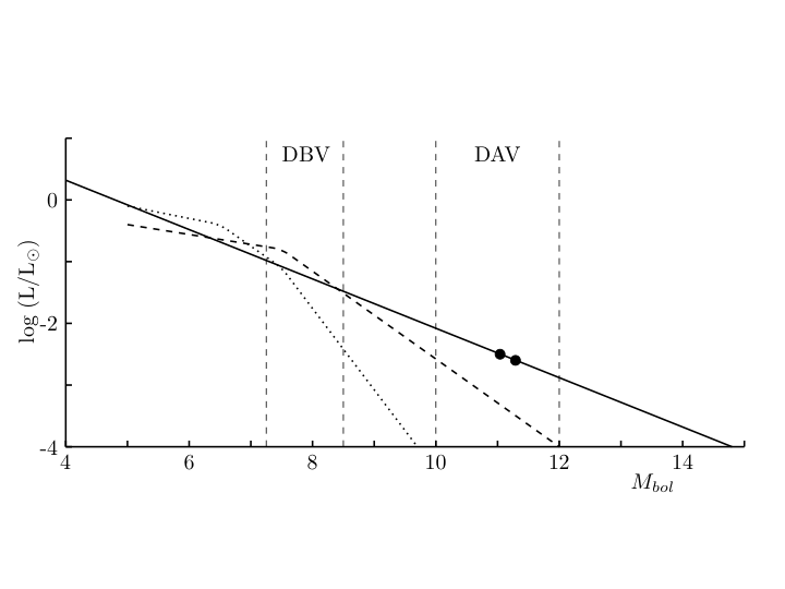
Figure 1: Evolution of the photonic (solid), nautrinic (dotted), and axionic (dashed) luminosities as the white dwarf fades. The vertical bands display the loci of the different families of variables.

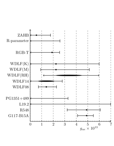
Figure 2: Axion-electron strengths obtained from different stellar constraints.

G117-B15A is a ZZ Ceti star discovered by [McGraw & Robinson (1976), McGraw & Robinson (1976)] that has been monitored since then. The first measurement of $\dot{P}$ gave a value that was a factor two larger than expected ([kepl91, Kepler et al., 1991]). The temperature of such star is low enough to neglect the radial term of Eq. 4 and the influence of neutrinos. These two facts led to [Isern et al.(1992), Isern et al., (1992)] to postulate axions of the DSKZ type with $g_{\rm ae}\approx 2.2\times 10^{-13}$ as responsible of the anomalous cooling. The analysis of [Córsico et al.(2001), Córsico et al., (2001)] and [bisc08, Bischoff-Kim et al., (2008)] showed that the presence of axions accelerates the drift but not changes the period of pulsation. The most recent estimation of the drift of the 215 s pulsation period is $\dot{P}_{\rm obs}=(4.07\pm 0.61)\times 10^{-15}$ s s^-1 ([kepl12, Kepler et al., 2012]), which suggests $g_{\rm ae}=4.9\times 10^{-13}$ (Fig. 2) from full model fitting ([C0́rsico et al.(2012a), Córsico et al., 2012a]).

Similar anomalous drifts have been found in R548, the ZZ Ceti star itself ([Mukadam et al. (2013), Mukadam et al., 2013]), and in L19.2 ([Sullivan & Chote (2015), Sullivan & Chote, 2015]), which could be accounted introducing axions with $g_{\rm ae}\times 10^{13}=4.8$ and $<7$ respectively ([Córsico et al.(2012b), Córsico et al., 2012b]; [Córsico et al. (2016), Córsico et al., 2016 ]).

These analysis indicate that the cooling rate is larger than expected if the pulsation modes are trapped in the outer envelope. This poses a problem since the trapping strongly depends on the detailed chemical gradients and the chemical structure of these layers, which are built during the AGB phase, is very sensitive to the methods used to treat convection and pulses during this epoch. Other problems come from the fact that these regions are partially degenerate and not all the physical inputs, specially axion emissivities, are correctly computed in this regime. Furthermore, there are still many uncertainties in the equation of state and opacities.

In the case of DB white dwarfs the drift has been measured in PG1351+489 ([Redaelli et al. (2011), Redaelli et al., 2011]), $\dot{P}_{\rm obs}=(2.0\pm 0.9)\times 10^{-13}$ s s^-1, which provides a bound of $g_{ae}\times 10^{13}<3.3$ ([Battich et al. (2016), Battich et al., 2016]). See Figure 2. Notice that at these temperatures, neutrinos are still active and their emission can be affected by axions or even by the existence of a hypothetical magnetic momentum.

4 The luminosity function

The luminosity function (LF) is defined as the number density of white dwarfs of a given luminosity per unit magnitude interval:

$$n\left(L\right)=\int\limits_{{M_{l}}}^{{M_{u}}}{\Phi\left(M\right)\Psi\left({{T_{G}}-{t_{cool}}-{t_{ps}}}\right){\tau_{cool}}dM}$$ (6)

where $M$ is the mass of the parent star (for convenience all white dwarfs are labeled with the mass of the zero age main sequence progenitor), $t_{cool}$ is the cooling time down to luminosity $L$, $\tau_{cool}=dt/dM_{bol}$ is the characteristic cooling time of the white dwarf, $t_{ps}$ is the lifetime of the progenitor of the white dwarf and $T_{G}$ is the age of the Galaxy or the population under study, and $M_{u}$ and $M_{l}$ are the maximum and the minimum mass of the main sequence stars able to produce a white dwarf, therefore $M_{l}$ satisfies the condition $T_{G}=t_{cool}(L,M_{l})+t_{ps}(M_{l})$. $\Phi(M)$ is the initial mass function and $\Psi(t)$ is the star formation rate (SFR) of the population under consideration. Additionally, hidden, there is an initial-final mass function connecting the properties of the progenitor with those of the white dwarf. In order to compare theory with observations, and since the total density of white dwarfs is not yet well known, the computed luminosity function is usually normalized to the bin with the smaller error bar, usually $\log L/L_{\odot}\simeq 3$.

This equation contains three sets of terms, the observational ones, $n(L)$, the stellar ones, $t_{\rm cool},\tau_{\rm cool},t_{\rm PS},M_{\rm U},M_{\rm i}$, plus the initial final mass function ([Catalan et al. (2008), Catalan et al., 2008]), and the galactic ones $\Phi$ and $\Psi$.

The first empirical luminosity function was obtained by [Weidemann (1968), Weidemann (1968)] and was improved by several authors during ninetees (Figure 4) proving in this way that the evolution of white dwarfs was just a cooling process and that there was a cut-off in the distribution caused by the finite age of the Galaxy. The position of the cut-off is sensitive to the cooling rate and, consequently, it can be used to constrain any new theory or hypothesis implying the introduction of an additional source or sink of energy. However the low number of stars in the samples, few hundreds, and the uncertainties in the position of the cut-off prevented anything else than obtaining upper bounds.

Figure 3: Luminosity functions obtained before the large cosmological surveys – [Liebert, Dahn & Monet (1988), Liebert, Dahn & Monet (1988)], full circles; [Evans (1992), Evans (1992)], full squares; [Oswalt et al. (1996), Oswalt et al., (1996)], open triangles; [Legget, Ruiz & Bergeron (1998), Legget et al., (1998)], open diamonds; [Knox, Hawkins & Hambly (1999), Knox, Hawkins & Hambly (1999)], open circles.

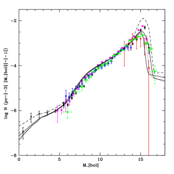
Figure 4: Luminosity functions obtained from the SDSS catalogue: Black solid squares ([Harris et al. (2006), Harris et al., 2006]), open blue squares, only DAs ([DeGennaro et al. (2008), DeGennaro et al., 2008]), black crosses ([krze09, Krzesinski et al., 2009]), and green stars ([Munn et al. (2017), Munn et al., 2017]). Magenta stars were obtained from the SCSS catalogue ([Rowell & Hambly (2011), Rowell & Hambly (2011)]) and contain DA and non–DA stars.

The advent of large cosmological surveys like the Sloan Digital Sky Survey (SDSS) and the Super COSMOS Sky Survey, both completely independent, introduced a noticeable improvement in the precision and accuracy of the luminosity function since they allowed to increase the sample size to several thousands of stars. Figure 4 displays both functions normalized to the $M_{\rm bol}\approx 12$ bin. As can be seen, they nearly coincide over a large part of the brightness interval. At large brightness, $M_{\rm bol}<6$, both luminosity functions show a large dispersion, not plotted in the figure, as a consequence of the fact that the proper motion method is not appropriate there. One way to circumvent this problem relies on the UV-excess technique ([krze09, Krzsinski et al. 2009]). The results obtained in this way are represented by black crosses after matching their dim region with the corresponding bright segment of the [Harris et al. (2006), Harris et al. (2006)] distribution. As a complement, the luminosity function of the dimmest white dwarfs obtained by [Legget, Ruiz & Bergeron (1998), Legget et al. (1998)] has been included (red triangles). The discrepancies at low luminosities are due to the difficulty to separate DAs from non-DAs and to the different behavior of the envelope.

The quality of this new luminosity functions allowed, for the first time, to determine their shape and to use the slope as a tool to test new physical theories. If an additional source or sink of energy is added, the characteristic cooling time is modified and its imprint appears in the luminosity function, as can be seen in Fig. 4, where a change of slope is evident at magnitudes $M_{\rm bol}\sim 8$. This change is caused by the transition from a cooling dominated by neutrinos to one dominated by photons. As an example, this technique was used by [Isern et al.(2008), Isern et al., (2008)] to suggest that axions of the DFSZ type could be contributing to the cooling of white dwarfs.

The main problem when using Eq. 6 is that the star formation rate has to be obtained independently from white dwarfs in order to break the degeneracy between the galactic properties and stellar models. Fortunately, the luminosity function has an important property. The shape of the bright branch, stars brighter than $M_{bol}\approx 13$, is almost independent of the assumed star formation rate as it can be seen in Fig. 4 where several theoretical white dwarf luminosity functions are displayed. The two solid black lines have been obtained assuming a constant SFR but two ages of the Galaxy, 10 and 13 Gyr respectively, the dashed line assuming a decreasing exponential SFR, $\Psi\propto\exp(-t/\tau),\,\tau=3\,{\rm Gyr}$, where $t$ is the age of the Galaxy, and the dotted line assuming an almost constant SFR with an exponentially decreasing tail that represents models where the star formation propagated from the center to the periphery, $\Psi\propto(1+\exp[(t-t_{0})/\tau])^{-1},\tau=3\,{\rm Gyr},\,t_{0}=10\,{\rm Gyr}$, where $t$ is the looking back time. As can be seen, in the region $M_{\rm bol}\approx 6-13$, all luminosity functions overlap as far as the SFR is smooth enough. The differences due to the shape of the SFR only appear in the regions containing cool or very bright white dwarfs. Unfortunately, the observational uncertainties in these regions prevent at present to discriminate among the different possibilities.

This behavior can be understood in the following way: Eq. (6) can be written as:

$$n\left(l\right)\propto\left\langle{{\tau_{cool}}}\right\rangle\int\limits_{{M_{i}}}^{{M_{\max}}}{\Phi\left(M\right)\Psi\left(T_{G}-t_{cool}-t_{ps}\right)}dM$$ (7)

Restricting this equation to the bright white dwarfs – namely, those for which $t_{\rm cool}$ is small – the lower limit of the integral is satisfied by low-mass stars and, as a consequence of the strong dependence of the main sequence lifetimes with mass, it adopts a value that is almost independent of the luminosity under consideration. Therefore, if $\Psi$ is a well-behaved function and $T_{G}$ is large enough, the lower limit is almost independent of the luminosity, and the value of the integral is incorporated into the normalization constant in such a way that the shape of the luminosity function only depends on the averaged physical properties of the white dwarfs ([iser08, Isern & García-Berro, 2008]). This average is dominated by low mass white dwarfs and, as far as the mass spectrum is not strongly perturbed by the adopted star formation or the initial mass function, it is representative of the intrinsic properties of white dwarfs ([Isern et al. (2009), Isern et al., 2009]). This shape, however, can be modified by a recent burst of star formation since, in this case, low-mass main sequence stars have no time to become white dwarfs and $M_{I}$ in Eq. 7 becomes luminosity dependent. On the contrary, if the burst is old enough, the corresponding luminosity functions are barely modified.

Another important property is that in the bright region considered here, the slope of the relationship between the luminosity and the core temperature of DA and non–DA white dwarfs almost coincide, and both luminosity functions almost overlap in this luminosity interval after normalization. This is the reason why the luminosity function of [DeGennaro et al. (2008), DeGennaro et al., (2008)] containing only DAs coincidesafter normalization with those containing DAs and non–DAs as it can be seen in Fig. 4. Therefore, Eq. 7 offers the possibility to use the slope of the bright branch of the luminosity function to detect the presence of unexpected additional sinks or sources of energy in white dwarfs. In the case of axions, this method was used for the first time by [Isern & García-Berro (2008), Isern et al.. (2008)] who obtained $g_{ae}=(1.4^{+0.9}_{-0.8})\times 10^{-13}$, see WDLF08 label in Fig. 2, using a preliminary version of the Harris loc cit. [Miller Bertolami et al. (2014), Miller Bertolami et al. (2014)] reexamined this result using all the luminosity functions of Fig. 4 (but with a consolidated Harris loc cit. luminosity function) and with a self consistent treatment of the neutrino cooling and concluded that DFSZ axions with a coupling constant $g_{ae}$ in the range of $(0.7-2.1)\times 10^{-13}$ could exist (WDLF14 label in Fig.2). All these results, however, have to be regarded as qualitative, since the uncertainties plaguing the determination of both, observed and computed, luminosity functions are still large.

Given the degeneracy between the stellar and galactic terms in Eq. 7, it is natural to wonder if the changes in the shape of the luminosity function attributed to axions are an artifact introduced by the star formation rate. One way to break this degeneracy and decide if it is necessary to introduce or not new physical effects is to examine the luminosity function of populations that have different formation histories. If axions exist and can modify the cooling of white dwarfs, their imprint will be present in all the luminosity functions at roughly the same luminosities. Furthermore, it is well known that the adopted white dwarf scale height above the galactic plane s has a noticeable effect on the shape of the luminosity function ([García-Berro et al.(1988), García-Berro et al., 1988];[Harris et al. (2006), Harris et al., 2006];[Kilic et al. (2017, Kilic et al., 1917]). This argument reinforces the convenience of analyzing the luminosity function of white dwarfs with different scale heights and independent star formation histories ([Isern et al. (2018), Isern et al., 2018]).

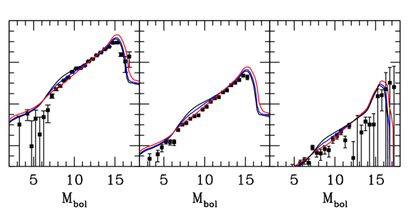
Figure 5: Luminosity functions of DA and non-DA white dwarfs of the thin and thick discs and halo [[Rowell & Hambly (2011), Rowell & Hambley 2011]]. The black line represent the case without axions. The blue and red lines correspond to the cases where DFSZ axions with coupling constants $g_{ae}\times 10^{13}=2.24$ and $4.48$ are included in the cooling model .

[Rowell & Hambly (2011), Rowell & Hambly (2011)] provided, for the first time, a luminosity function for the thin and thick disks and noticeably improved that of the halo (Fig. 5). Table 1 shows how the discrepancies between theoretical calculations and observations decrease in all three cases when axions are included. The fit favors axions within the interval $g_{ae}=(2.24-4.48)\times 10^{-13}$ with some tension between the halo and the disk results, although the $2\,\sigma$ bounds are compatible. See Fig. 2, label WDLF(RH).

Table 1: Reduced $\chi^{2}$ obtained from the fitting of the observed white dwarf luminosity functions in the brightness interval $6\,<\,M_{\rm bol}\,<\,12.5$ with different intensities of the coupling between electrons and axions [Isern et al. 2018].

$g_{\rm ae}\times 10^{13}$	0.00	1.12	2.24	4.48
$m_{\rm a}\cos^{2}\beta$ (meV)	0	4	8	16
Rowell & Hambly (2011)
thin disk	18.59	15.33	7.33	21.52
thick disk	30.72	26.61	11.73	1.43
halo	3.31	2.94	2.36	1.87
Munn et al. (2017)
thin+thick disk	4.89	2.87	1.46	6.13
halo	2.46	1.50	0.65	1.42
Kilic et al. (2017)
$\Phi_{200-900}$	3.25	2.09	1.05	6.11
$\Phi_{200-700}$	3.53	2.32	1.14	5.80
$\Phi_{200-500}$	4.02	2.73	1.28	2.26
$\Phi_{300}$	6.11	4.95	2.26	4.98

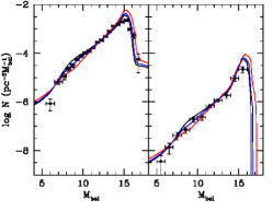
Figure 6: Luminosity functions of DA and nDA white dwarfs belonging to the disk (thin and thick) and the halo (Munn et al., 2017). The meaning of the solid lines is the same as in Fig. 5.

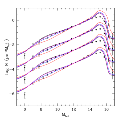
Figure 7: White dwarf luminosity functions of the disk assuming different scale heights as proposed by Kilic et al. (2017). From top to bottom $\Phi_{200-900}+3$, $\Phi_{200-700}+2$, $\Phi_{200-500}+1$ and $\Phi_{300}$. Solid lines correspond to $g_{ae}\times 10^{13}=0,1.12,2.24,4.48$ (black, magenta, blue, red, respectively). The dashed line corresponds to a case with no axions and an SFR constant plus an exponential tail as in Fig 4.

Munn et al. (2017) improved the Harris et al. (2006) luminosity function resolving the peak and increasing the precision of the brighter branch assuming a constant scale height above the Galactic plane. They also computed the luminosity function for the halo selecting white dwarfs with $200\leq v_{\rm tan}\leq 500$ km s^-1. As before, the inclusion of axions improves the concordance between theory and observations both in the disk and the halo. The best fit is obtained for $g_{ae}\approx 2.24\times 10^{-13}$, label WDLF(M) Fig. 2, with ($2\,\sigma$) upper bounds of $g_{ae}<(4.2\,{\rm and}\,14)\times 10^{-13}$ coming, respectively, from the disk and halo luminosity functions.

Kilic et al. (2017) reexamined the Munn et al. (2017) data assuming three variable scale heights above the galactic plane going linearly from 200 pc now to 900, 700 and 500 pc in the past ,respectively, and one with a fixed scale height of 300 pc. They concluded that the slight discrepancies in the region $6\leq M_{\rm bol}\leq 12.5$ were caused by the use of a fixed scale height. This argument is correct but, as it was shown by Isern et al (2018), see Fig. 7, the inclusion of axions improves the agreement. In these cases the best fit was also around $g_{ae}\approx 2.24\times 10^{-13}$, Table 1, and a $2\,\sigma$ global upper bound $g_{ae}<6\times 10^{-13}$ (Fig. 2, label WDLF(K)).

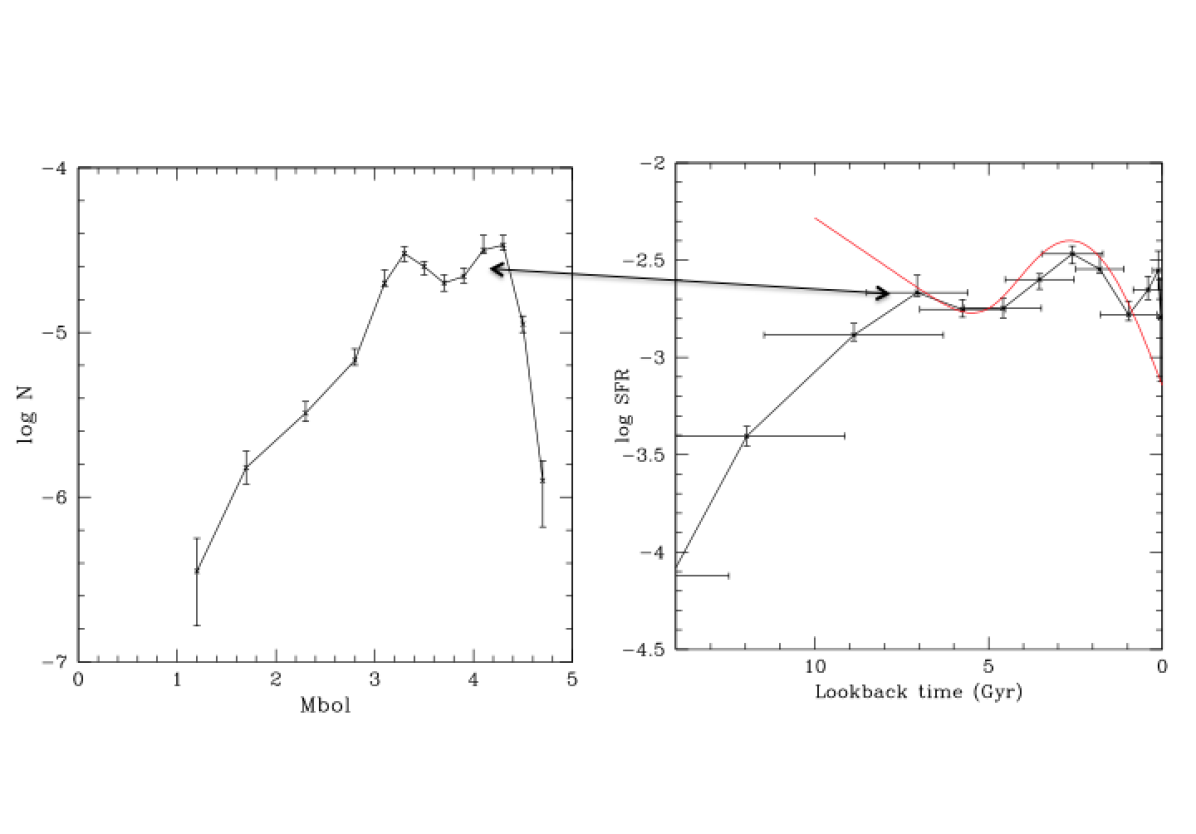
Figure 8: Left panel: empirical luminosity function of massive ($M_{\rm WD}\leq M/M_{\odot}\leq 1.1$) DA white dwarfs in the solar neighborhood ([Tremblay et al.(2019), Tremblay et al., 2019]). Right panel: in black, the corresponding star formation rate ([Isern (2019), Isern, 2019]), in red, the Galactic disc star formation ([Mor et al.(2019), Mor et al., 2019].

Recently a second possibility has appeared. [Tremblay et al.(2019), Tremblay et al., (2019)] have been able to build a reliable and precise luminosity function of massive white dwarfs that belong to the solar neighborhood ($d\leq 100$ pc) using the data provided by Gaia (Fig. 8, left panel). If the luminosity function, Eq. 6, is restricted to massive white dwarfs, i.e. those for which it is possible to neglect the lifetime of the progenitor in front of the cooling time, and $\Psi$ is smooth enough, the age of any bin and the star formation rate corresponding to this time can be computed as

$$\left\langle t\right\rangle=\frac{{\int\limits_{\Delta M}{\Phi(M)tdM}}}{{\int\limits_{\Delta M}{\Phi(M)dM}}}$$ (8)

and

$$\left\langle\Psi\right\rangle=\frac{{n(l)}\Delta l}{{\int\limits_{\Delta M}{\Phi\left(M\right)\Delta{t_{cool}}\left({l,M}\right)dM}}}$$ (9)

with $\Delta{t_{cool}}={t_{cool}}\left({l+0.5\Delta l,M}\right)-{t_{cool}}\left({l-0.5\Delta l,M}\right)$, $l=-\log(L/L_{\odot})$ and $\Delta l$ the width of the luminosity function bin (Isern, 2019) and this allows to reconstruct the star formation history of the solar neighborhood (Fig. 8, right panel). The star formation rate obtained in this way is not constant or monotonically decreasing as it is often assumed. It grew quickly in the past, during the first epochs of the Galaxy, it roughly stabilized and started to decrease 7 to 6 Gyr ago. A noticeable feature is a prominent peak centered around 2.5 Gyr ago, the exact position being model depending.

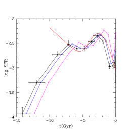
Figure 9: Star formation rate (M_⊙Gyr^-1pc^-3) in the solar neighborhood obtained from massive white dwarfs assuming no axions (black line). The blue and magenta lines correspond to the case when axions are present and have a coupling constant $g_{ae}=2.24\,{\rm and}\,4.48\times 10^{-13}$, respectively. The red line corresponds to the star formation rate obtained by [Mor et al.(2019), Mor et al., (2019)].

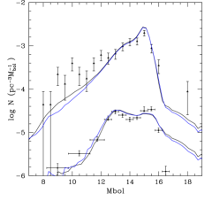
Figure 10: Theoretical versus empirical luminosity functions for massive and all white dwarfs. The empirical ones are from [Tremblay et al.(2019), Tremblay et al.(2019)] and [Oswalt et al., (2017), Oswalt et al.(2017)] respectively.The theoretical ones were obtained with the star formation rates of Fig. 10 with $g_{ae}=0$ (black lines) and $2.24\times 10^{-13}$ (blue lines).

The existing degeneracy between galactic properties and evolutionary models imply that different stellar models can lead to different star formation histories, for which reason it is necessary to compare these results with others obtained independently. [mor18, Mor et al., (2018)] computed the star formation history of the Galactic disk using main sequence stars from the Gaia DR2 and the Besançon Galaxy Model. Since this function is expressed in stars per unit of disk surface it has been divided by an arbitrary and constant height scale above the galactic plane (red line, Fig. 10). As it can be seen both methods, local and galactic, predict a concordant burst of star formation $\sim 2.5$ Gyr ago but diverge at early times. This divergence may have several origins, a local delay in starting the star formation process, a different behavior of the outer and inner disks, a vertical dilution caused by a galaxy collision or just the conversion of DA white dwarfs into non-DAs. The peak that appears at $\sim 0.2$ Gyr is in the limit of applicability of the method and deserves more attention.

Figure 10 displays the star formation rate obtained when including axions (and crystallization sedimentation effects) in the cooling models. As it can be seen, the SFRs obtained in this way have the same behavior, but they are displaced towards shorter ages and larger rates thus providing an additional way to discriminate among theoretical models. Figure 10 displays a test of consistency where the SFR obtained from the luminosity function of the massive ones is used to compute the total one. The agreement between theory and observations is reasonable taking into account that observations were obtained independently and that the results are very sensitive to the DA/nDA properties as well as to the adopted initial mass function and initial final mass relationship. The excesses around $M_{\rm bol}\sim 9-10$ could be due to recent bursts of star formation not resolved by the present binning of the massive luminosity function and, as mentioned before, deserves a detailed analysis. Figure 10 also shows that values of $g_{ae}\hbox{\lower 3.44444pt\hbox{$\,\buildrel>\over{\sim}\,$}}3\times 10^{-13}$ are not compatible with the results obtained by Mor et al., (2019).

5 Discussion and conclusions

The two methods presented here are complementary since they measure the cooling rate of the same object using different phenomenologies. One, the drift of the pulsation period, applies to individual stars, while the other, the luminosity function, applies to the population ensemble. As it is evident from Fig. 2, there is some tension between both sets of data but, given the uncertainties, they can be considered as qualitatively concordant.

Axions with the properties described here not only would perturb the cooling of white dwarfs but they would also modify in a subtle way the evolution of other kind of stars. An extensive review can be found in [Giannotti et al., 2017, Giannotti et al., (2017)], while [Sedrakian (2019, Sedrakian (2019)] provides a recent analysis of the cooling by DFSZ axions of the neutron star in Cas A. Here only the two more restrictive tests are presented.

The luminosity of a star in the red giant branch depends on the mass of its core and is due to the hydrogen burning in a thin shell surrounding it ([Paczynski, B. (1970), Paczynski, 1970]). Thus, the luminosity grows with the core until He is ignited in the center. If axions were present, the core would be more massive than in the standard case and, consequently, the tip of the red giant branch would be brighter. Obviously, since H-burning occurs via CNO-cycle, this luminosity depends on the metallicity. The analysis of the red tip in M5 suggested the necessity of an extra cooling source. If this source were axions, the electron coupling constant should be $g_{ae}\sim 1.9\times 10^{-13}$ ([Viaux et al., (2013), Viaux et al., 2013]), but a similar analysis performed on M3 did not find the necessity of an extra cooling term and provided a more stringent upper bound of $g_{ae}<2.57\times 10^{-13}$ ([Straniero et al., (2018), Straniero et al., 2018]). A similar bound has also been obtained using a set of 50 globular clusters ([Arceo-Diaz et al., (2019), Arceo-Diaz et al., 2019]). In Fig. 2 this bound and the hint found in M5 are represented by the RGB-T line. A detailed analysis of the existing uncertainties can be found in [Serenelli et al. (2017), Serenelli et al., (2017)].

The evolution of HB stars provides additional observational tests. The number of stars in a given region of the HR diagram is roughly proportional to the time spent in it. Since HB stars are the direct descendants of red giant stars, the ratio between the number of HB stars, $N_{\rm HB}$, and the red giants, $N_{\rm RGB}$, in a cluster should satisfy the relationship $R=N_{\rm HB}/N_{\rm RGB}=\Delta t_{\rm HB}/\Delta_{\rm RGB}$ and, since the densities and temperatures of both populations are very different, the inclusion of the axion emission should strongly perturb these quantities. This parameter has been measured in a large sample of globular clusters and is fairly constant at low metallicities, $R_{\rm av}=1.39\pm 0.03$ ([Salaris et al., (2004), Salaris et al., 2004]).

[Ayala et al., (2014), Ayala et al., (2014)] and [Straniero et al., (2015), Straniero et al., (2015)] examined the influence of axions in this case and found that the best fit to the parameter R was obtained for $g_{a\gamma}=0.29\pm 0.18\times 10^{-10}$ GeV^-1, i.e. that it was necessary an extra cooling factor, with an upper bound of $g_{a\gamma}<0.66\times 10^{-10}$ GeV^-1. In terms of the mass of the axion, these values translate to $0.12$ eV and $<0.2$ eV, respectively, in the case of the KSVZ axions. Since they did not include bremsstrahlung with electrons, that strongly affects the evolution of RGB stars, it is not possible to extrapolate these values to the DFSZ case. However, in an updated version, taking into account the axion-electron interaction, [Straniero et al., (2018), Straniero et al., (2018)] obtained $g_{a\gamma}<0.5\times 10^{-10}$ GeV^-1 and $g_{ae}<2.6\times 10^{-13}$ (these values are represented in Fig. 2). These results, however, strongly depend on the assumed He abundance in the cluster.

The Zero Age Horizontal Branch provides an additional test. If the axion-electron interaction is operating in RGB stars, the core is larger and the luminosity of HB stars too. [Straniero et al., (2018), Straniero et al., (2018)] examined this case and found a best fit at $g_{ae}=0.54\times 10^{-13}$ and a bound at $g_{ae}<1.78\times 10^{-13}$. These values are plotted in Fig. 2.

Certainly, the deviations represented in Fig. 2 have a small statistical significance, but taken together they suggest that stars loose energy more efficiently than expected. Axions of the DFSZ type, with a mass of few meV could do the job, although other possibilities are open. For instance an ALP with $g_{ae}\sim 1.5\times 10^{-13}$ and $g_{a\gamma}\sim 1.4\times 10^{-11}$ GeV^-1 ([Giannotti et al., 2016, Giannotti et al., 2016]). It is evident from this discussion that a direct detection is necessary to prove the existence of axions and that white dwarfs provide an interesting hint on where to search. IAXO is a future experiment designed to detect the emission of axions by the Sun ([Irastorza et al., (2011), Irastorza et al., 2011]) that will have enough sensitivity to detect axions of the DFSZ type and mass $\hbox{\lower 3.44444pt\hbox{$\,\buildrel>\over{\sim}\,$}}3$ meV, according to the calculations of [Redondo (2013, Redondo, (2013)].

Thanks to the data that is providing Gaia and will provide the LSST as well as other instruments, white dwarfs will become in a next future one of the best characterized populations of the Galaxy, and this will convert them into an excellent laboratory to explore new ideas in Physics.

References

- [Althaus et al.(2010)] Althaus, L.G.., Córsico, A.H., Isern, J., & García-Berro, E. 2010, AAR, 18, 471
- [Altherr et al.(1994)] Altherr, T., Petitgirard, E. & Gaztelarrutia, T. 1994, Astroparticle Phys., 2, 175
- [Arceo-Diaz et al., (2019)] Arceo-Diaz, S., Schroeder, K.-P., Zuber, K., et al. 2019, ArXiv: 1910.10568
- [Ayala et al., (2014)] Ayala, A., Dominguez, I., Giannotti, M., Mirizzi, A., & Straniero, O. 2014, Phys. Rev. Lett., 113, 191302
- [Battich et al. (2016)] Battich, T., Córsico, A.H., Althaus, L.G., Miller Bertolami, M.M 2016, JCAP. 8, 62
- [Bertone & Fairbairn (2000)] Bertone, G., & Fairbairn, M. 2008, Phys. Rev. D, 77, 043515
- [Bischoff-Kim et al.(2008)] Bischoff-Kim, A., Montgomery, M.H., & Winget, D.E. 2008, ApJ,675, 1512
- [Blinnikov & Dunina-Barkovskaya (1994)] Blinnikov, S.I. & Dunina-Barkovskaya, N.V. 1994, MNRAS, 266, 289
- [Catalan et al. (2008)] Catalan, S. et al. 2008, MNRAS, 387, 69
- [Córsico et al.(2001)] Córsico, A.H., Benvenuto, O.G., Althaus, L.G., Isern, J., & García-Berro, E. 1989, New. Astron., 6, 197
- [C0́rsico et al.(2012a)] Córsico, A.H., Altahus, L.G., Miller Bertolami, M.M., Romero, A.D., García-Berro, E., Isern, J., Kepler, S.O. 2012a MNRAS, 424, 2792
- [Córsico et al.(2012b)] Córsico, A.H., Altahus, L.G., Romero, A.D., Mukadam, A.S., García-Berro, E., Isern, J., Kepler, S.O., Corti, M.A. 2012 b JCAP,12, 10
- [Córsico et al. (2016)] Córsico, A.H. et al. 2016, JCAP, 7, 36
- [D’Antona & Mazzitelli (1989)] D’Antona, F.& Mazzitelli, I. 1989, ApJ, 347, 934
- [DeGennaro et al. (2008)] DeGennaro, S. et al. 2008, AJ, 135,1
- [Dias et al., (2014)] Dias, A.G., Machado, A.C.B., Nishi, C.C., Ringwald, A. & Vandrevange, P. 2014, JHEP, 2014,37
- [Dine, Fishler & Srednick (1981)] Dine, M., Fishler, W. & Srednick, M 1981, Phys. Lett. B, 104, 109
- [Dreiner et al.(2013)] Dreiner, H.K., Fortin, J-F., Isern, J., & Ubaldi L. 2013, Phys. Rev. D, 88, 043517
- [Evans (1992)] Evans, D.W. 1992, MNRAS, 255,521
- [Fontaine et al.(2001)] Fontaine, G., Brassard, P., & Bergeron, P. 2001, PASP, 113, 409
- [Freese (1984)] Freese, K. 1984, ApJ, 286, 216
- [García-Berro et al.(1988)] García-Berro, E., Hernanz, M., Mochkovitch, R. Isern, J., 1988, A&A, 193, 141
- [García-Berro et al.(1995)] García-Berro, E., Hernanz, M., Isern, J., & Mochkovitch, R. 1995, MNRAS, 277, 801
- [García-Berro, & Oswalt (2016)] García-Berro, E., & Oswalt, T.D.. 2016, New Astron. Rev, 72, 1
- [Giannotti et al., 2016] Giannotti, M., Irastorza, I.G., Redondo, ,J., & Ringwald, A. 2016, JCAP, 05, 057
- [Giannotti et al., 2017] Giannotti, M., Irastorza, I.G., Redondo, ,J., Ringwald, A. & Saikawa, K. 2017, JCAP, 10, 010
- [Giddings & Mangano (2008)] Giddings, S.B., & Mangano, M.L. 2008, Phys.Rev.D, 78, 035009
- [Hansen (2004)] Hansen, B.M. 2004, Phys. Rep., 399, 1
- [Harris et al. (2006)] Harris, H.C. et al. 2006, AJ, 131, 571
- [Iben & Tutukov (1984)] Iben, I., & Tutukov, A.V. 1984, ApJ, 282, 615
- [Irastorza et al., (2011)] Irastorza, I.G., et al. 2011, JCAP, 06, 013
- [Isern (2019)] Isern, J. 2019, ApJL, 878, L11
- [Isern et al. (2009)] Isern, J., Catalan, S., García-Berro, E. & Torres, S. 2009, J. Phys. Conf. Series, 172, 012005
- [Isern & García-Berro (2008)] Isern, J., & García-Berro, E. 2008, MemSAI, 79, 545
- [Isern et al., (2010)] Isern, J., García-Berro, E., Altahus, L.G. & Córsico, L. H. 2010, A & A, 512, 86
- [Isern et al.(1998)] Isern, J., García-Berro, E., Hernanz, M. & Mochkovitch, R. 1998, Jour. Phys. Cond. Mat, 10, 11263
- [Isern et al.(2008)] Isern, J., García-Berro, E., Torres, S. & Catalán, S. 2008, ApJL, 682, L100
- [Isern et al. (2018)] Isern, J., García-Berro, E., Torres, S., Cojocaru, R. & Catalán, S. 2018, MNRAS, 478, 2569
- [Isern et al.(1992)] Isern, J., Hernanz, M., & García-Berro, E. 1992, ApJL, 392, L23
- [Itoh et al. (1996)] Itoh, N., Hayashi, H., Nishikawa, A. & Kohyama, Y. 1988, ApJS, 102, 411
- [Kilic et al. (2017] Kilic, M., Munn, J.A., Harris, H.C. et al. 2017, ApJ, 837,162
- [Knox, Hawkins & Hambly (1999)] Knox, R.A., Hawkins, M.R.S., & Hambly, N.C. 1999, MNRAS, 306, 736
- [Koester & Shoenberner (1986)] Koester, D. & Shoenberner, D. 1986, A&A, 154, 125
- [Krzesinski et al. (2009)] Krzesinski, J., et al. 2009, A&A, 508,339
- [Malec, & Besiada (2001)] Malec, B., & Besiada, M. 2001, Acta Phys. Pol. B, 32, 3683
- [McGraw & Robinson (1976)] McGraw, J.T. & Robinson, E.L. 1976, ApJ, 205, 155
- [Miller Bertolami et al. (2014)] Miller Bertolami, M.M., Mlendez, B., Althaus, L.G. & Isern, J. 2014, JCAP, 1410, 069
- [Mor et al.(2019)] Mor, R., Robin, A.C., Figueras, F., Roca-Fàbrega, S., & Luri, X. 2019, A&A 624, L1
- [Mukadam et al. (2013)] Mukadam, A.S. et al. 2013, ApJ, 771, 17
- [Munn et al. (2017)] Munn, J.A. et al. 2017, AJ, 153, 10
- [Nakagawa et al. (1987)] Nakagawa, M, Kohyama, Y. & Itoh, N. 1987, ApJ, 322, 291
- [Nakagawa et al. (1988)] Nakagawa, M., Adachi, T., Kohyama, Y. & Itoh, N. 1988, ApJ, 326, 241
- [Legget, Ruiz & Bergeron (1998)] Legget, S. K., Ruiz, M.T., & Bergeron, P. 1998, ApJ, 497, 294
- [Liebert, Dahn & Monet (1988)] Liebert, J., Dahn, C.C., & Monet, D.G. 1988, ApJ,332, 891
- [Oswalt et al., (2017)] Oswalt, T.D., Holberg, J. & Sion, E. 2017, 20th European White Dwarf Workshop, Ed. P.-E. Tremblay et al., ASP Conference Series 509, 59
- [Oswalt et al. (1996)] Oswalt, T.D., Smith, J. A., Wood, M.A., & Hintzen, P.A. 1996, Nature 382, 692
- [Paczynski, B. (1970)] Paczynski, B. 1970, Acta Astron., 20, 287
- [Raffelt (1986)] Raffelt, G.G. 1986, Phys. Lett. B, 166, 402
- [Raffelt (1996)] Raffelt, G.G. 1996, in: K.K. Turekian, H.D. Holland & A.M. Davis (eds.), Stars as Laboratories of Fundamental Physics (University of Chicago Press).
- [Redaelli et al. (2011)] Redaelli, M., Kepler, S.O., Costa, J.E.S. et al. 2011, MNRAS, 415, 1220
- [Redondo (2013] Redondo, J. 2013, JCAP, 12,008
- [Ringwald, 2014] Ringwald, A. 2014, ArXive: 14070546