Enlarging Discriminative Power by Adding an Extra Class
in Unsupervised Domain Adaptation

Abstract

In this paper, we study the problem of unsupervised domain adaptation that aims at obtaining a prediction model for the target domain using labeled data from the source domain and unlabeled data from the target domain. There exists an array of recent research based on the idea of extracting features that are not only invariant for both domains but also provide high discriminative power for the target domain. In this paper, we propose an idea of empowering the discriminativeness: Adding a new, artificial class and training the model on the data together with the GAN-generated samples of the new class. The trained model based on the new class samples is capable of extracting the features that are more discriminative by repositioning data of current classes in the target domain and therefore drawing the decision boundaries more effectively. Our idea is highly generic so that it is compatible with many existing methods such as DANN, VADA, and DIRT-T. We conduct various experiments for the standard data commonly used for the evaluation of unsupervised domain adaptations and demonstrate that our algorithm achieves the SOTA performance for many scenarios.

1 Introduction

Deep neural networks have recently been used as a major way of achieving superb performance on various machine learning tasks, e.g., image classification [9], image generation [8], and speech recognition [1], just to name a few. However, it still leaves much to be desired when a network trained on a dataset from a specific data source is used for dataset from another data source. This domain shift and thus distribution mismatch frequently occurs in practice, and has been studied in the area of domain adaptation. The crucial ingredient in domain adaptation lies in transferring the knowledge from the source domain to the model used in the target domain.

(a) Domain-invariant feature
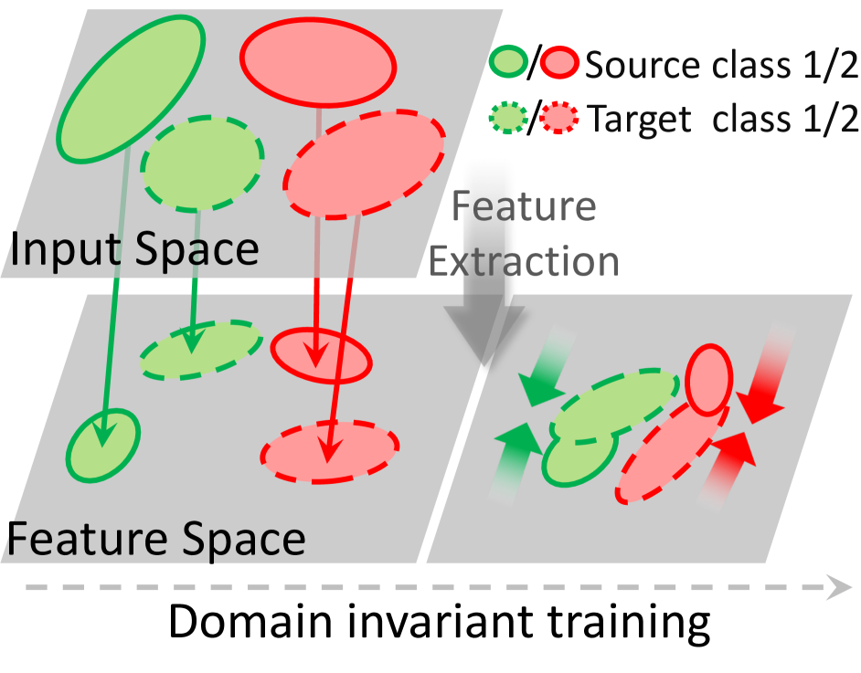
extraction

(b) Larger discriminative power:
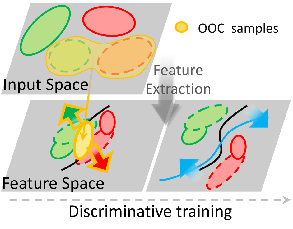
“fictitious” class and OOC samples.

Figure 1: Illustration on how GADA works. Each arrow in the feature space corresponds to the force that moves the extracted features or decision boundary. (a) describes how domain-invariant features are learned. (b) explains how discriminative features are extracted by utilizing out-of-class (OOC) samples. The OOC samples and $(K+1)^{\text{th}}$ class increase the distance between “real” clusters, which helps the classifier place the decision boundary in the low-density area easier.

In this paper, we consider the classification problem of unsupervised domain adaptation, where the trained model has no access to any label from the target domain. What a good domain adapation model has to have is two-fold. First, it is able to extract domain-invariant features that are present in both source and target domains, thereby aligning the feature space distributions between two different domains, e.g., [24, 12, 13, 22, 6, 7, 4]. Second, it has to have high discriminative power for the target domain task, which becomes possible by smartly mixing the following two operations: (i) extracting task-specific, discriminative features [23, 26, 11] and (ii) calibrating the extracted feature space so as to have a clearer separation among classes, e.g., moving the decision boundaries [21] (see Section 2 for more details).

Despite recent advances in unsupervised domain adaptation, there still exists non-negligible performance gap between domain adapted classifiers and fully-supervised classifiers, hinting a room for further improvement. In this paper, we focus on the second part of empowering the predictive model with more discriminativeness, whose key idea is as follows: Assuming that there are $K$ classes in the target data, we equip the model with an extra $(K+1)^{\text{th}}$ class. This extra class is constructed so as to contain the target samples, which we call out-of-class (OOC) samples throughout this paper, that fail to belong to any of $K$ classes. Feeding such OOC samples and classifying them into the $(K+1)^{\text{th}}$ class help to provide the classifier with new samples, thereby improving its feature extraction power in terms of discriminativeness. Figure 1 illustrates our idea, where to obtain the OOC samples, we train a generator based on a feature matching GAN [20]. We call our idea GADA (Generative Adversarial Domain Adaptation).

(a) DANN [7] (74.9%)

(b) GADA (99.0%)

Figure 2: Feature space comparison for the domain adaptation task SVHN $\rightarrow$ MNIST. The number in parenthesis corresponds to the classification accuracy.

This power of an extra class has already been verified in the area of semi-supervised learning [20, 5, 15]. Our contribution is to apply this idea to unsupervised domain adaptation in conjunction with necessary engineering components to be practically realized. To the best of our knowledge, this paper is the first to integrate the idea of adding an extra class with unsupervised domain adaptation. We comment that, compared to the case of semi-supervised learning, it is necessary to learn both the domain-invariant and the discriminative features, requiring to strike a good balance between those two in domain adaptation.

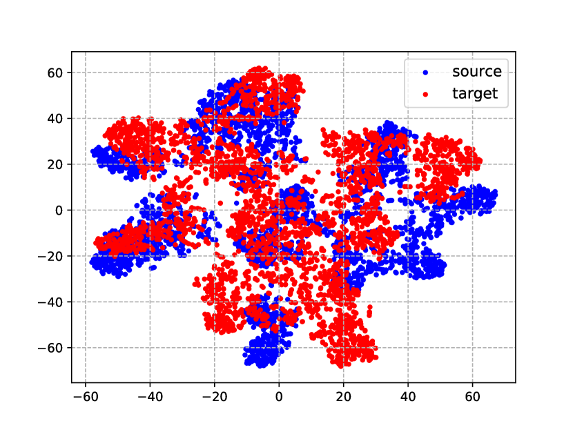
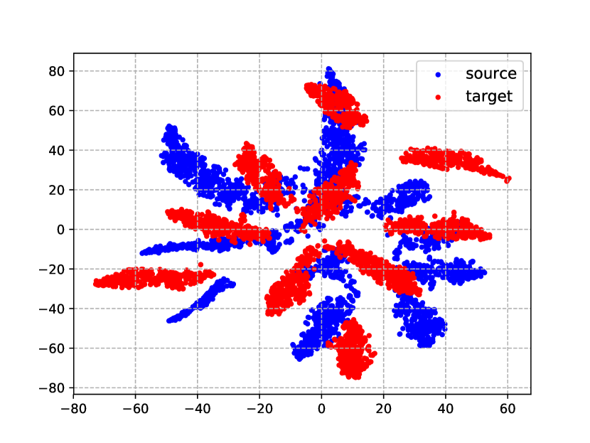
We highlight that our method is highly generic so as to be compatible with many existing methods. Figure 2 shows the feature space illustration, demonstrating the power of GADA, when used together with the notorious method, DANN [7]. As Figure 2 shows, we achieve a significant improvement in terms of accuracy and separability among the classes. We also show our integration power with two recent methods, VADA and DIRT-T [21], which are the methods that improve the model’s discriminative power. VADA aims to extract discriminative features better by employing smart loss functions in training, whereas DIRT-T refines the decision boundary for given extracted features. As shown later in Section 4, we achieve the best performance in the most difficult task MNIST $\rightarrow$ SVHN after the integration. This implies that (i) simply adding a new, fictitious class and training with generated samples as in GADA outperforms the VADA algorithm, and (ii) our idea is significantly synergic with a refining-based method DIRT-T.

We empirically prove the effects of our method by carrying out an extensive set of experiments where we observe that our method outperforms other state-of-the-art methods on four among six standard domain adaptation tasks, consisting of the datasets MNIST, SVHN, MNIST-M, DIGITS, CIFAR, and STL. Although the task SVHN $\rightarrow$ MNIST had a very high accuracy achieved by the existing methods, GADA is demonstrated to surpass all of them. As for MNIST $\rightarrow$ SVHN, which is known to be extremely challenging, we integrate our module with VADA [21] to yield an improvement of $13\%$ in terms of accuracy, thereby setting a new state-of-the-art benchmark.

2 Related Work

For presentational convenience, we present the related work by classifying them into two categories based on their emphasis on (i) extracting domain-invariant features and (ii) improving discriminativeness.

Extracing domain-invariant features

A collection of work [24, 12, 13, 22] aimed at aligning the feature space distributions of the source and target domains by minimizing the statistical discrepancy between their two distributions using different metrics. In [24, 12], maximum mean discrepancy (MMD) was used to align the high layer feature space. In [13], Joint MMD (JMMD) was used by defining the distance between the joint distributions of feature space for each layer one by one. In [22], the covariances of feature space were used as the discrepancy to be minimized. Different approaches include [6] and [17]. The authors in [17] proposed a method of minimizing the regularization loss between the source and target feature network parameters so as to have similar feature embeddings. DANN [6] used a domain adversarial neural network, where the feature extractor is trained to generate domain-invariant features using a gradient reversal layer, which inverses the sign of gradients from a domain discriminator.

Improving discriminativeness

The idea in DANN has been used as a key component in many subsequent studies [23, 26, 21, 11], which essentially modified the adversarial training architecture to acquire more discriminative power. Different from the end-to-end training in DANN, ADDA (Adversarial Discriminative Domain Adaptation) [23] divided the training into two stages: (a) normal supervised learning on a feature extractor and a feature classifier on the source domain, and (b) training the target domain’s feature extractor to output the features similar to the source domain’s. In [26], a semantic loss function is used to measure the distance between the centroids of the same class from different domains. Then, minimizing the semantic loss function ensures that the features in the same class from different domains will be mapped nearby. VADA (Virtual Adversarial Domain Adaptation) [21] add two loss functions to DANN to move the decision boundaries to low-density regions. DIRT-T [21] solves the non-conservative domain adaptation problem by applying an additional refinement process to the model trained by VADA.

We summarize other array of work designed for improving discriminativeness. Tri-training method [18] used high-quality pseudo-labeled samples to train an exclusive classifier for the target domains via ensemble neural networks. CoDA (Co-regularized Domain Adaptation) [11] increases the search space by introducing multiple feature embeddings using multiple networks, aligning the target distribution into each space and co-regularizing them to make the networks agree on their predictions. In GAGL (Generative Adversarial Guided Learning) [25], the authors used a generator trained with CMD (Central Moment Discrepancy) [27], similar to what we propose in this paper, in order to boost the classifier performance. However, their experiment results are far from the state-of-the-art performance.

Pixel-level approach

We have focused on the feature-level domain adaptation. There exist pixel-level approaches: In [3], the authors proposed to adapt the two domains in the pixel level. The works in [14] and [10] used Cycle GAN [28] to perform the pixel-level adaptation and integrate it with the feature-level domain adaptation in the same model to extract better domain-invariant features.

Bad GAN

The idea of using a $(K+1)^{\text{th}}$ output to improve the model performance was widely used in the semi-supervised learning problem [20, 5, 15]. The work in [20] was the first that introduces the $(K+1)^{\text{th}}$ output and apply it to the semi-supervised learning problems. Bad GAN [5] first theoretically and empirically proved the effectiveness of a bad generator in helping the classifier to learn, and then designed several loss functions as an attempt to generate bad samples. While the additional output proved its effects in semi-supervised learning, we utilize it to solve the problem of unsupervised domain adaptation in this paper.

3 Method

3.1 Unsupervised Domain Adaptation

The problem of unsupervised domain adaptation is formulated as follows. We are given the source dataset with labels $(\pazocal{X}_{S},\pazocal{Y}_{S})$ from the source domain $\pazocal{D}_{S}$ and the target dataset $\pazocal{X}_{T}$ from the target domain $\pazocal{D}_{T}$, but the target data has no labels. A domain shift between the two domains is assumed, i.e., $\pazocal{D}_{S}\neq\pazocal{D}_{T}$. The ultimate goal of unsupervised domain adaptation is to learn a good inference function on the target domain $f:\pazocal{X}_{T}\to\pazocal{Y}_{T}$ using the labeled source data $(\pazocal{X}_{S},\pazocal{Y}_{S})$ and the unlabeled target data $\pazocal{X}_{T}$.

3.2 GADA

In this section, we present our method, called GADA (Generative Adversarial Domain Adaptation), ranging from the overall network architecture to the detailed algorithm description.

Figure 3: Network architecture of GADA. Colored solid lines show the flows of source, target and generated data. Six different loss functions are used: (i) $\pazocal{L}_{d}$ updates $\theta_{D}$ and $\theta_{g}$ for domain-invariance; (ii) $\pazocal{L}_{c}$, $\pazocal{L}_{u}$, $\pazocal{L}_{e}$, and $\pazocal{L}_{v}$ updates $\theta_{g}$ and $\theta_{h}$ to extract discriminative features, and (iii) $\pazocal{L}_{g}$ updates the generator parameters $\theta_{G}$. The red arrows show the positions where the losses are computed (see Sections 3.2.2 and 3.2.3 for details).

3.2.1 Network Structure

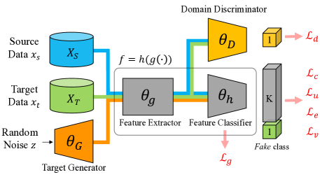
We illustrate the network structure of GADA in Figure 3, which consists of four major components C1-C4 as follows:

1. a feature extractor $g$ with parameters $\theta_{g}$

2. a feature classifier $h$ with parameters $\theta_{h}$

3. a domain discriminator $D$ with parameters $\theta_{D}$

4. a generator $G$ with parameters $\theta_{G}$

The feature extractor $g$ extracts the common features of the inputs from the source and target domains, while the feature classifier $h$ classifies the extracted features from $g$ and outputs the classification scores. The domain discriminator $D$ is a network with binary output, which indicates whether an input is from the source domain or the target domain. The key idea is that, if we are able to fool a smart discriminator $D$, i.e., making it fail to distinguish the input domains, the extracted features $g(X)$ become domain-invariant. A generator $G$ plays a role of generating the out-of-class (OOC) samples which differs from the data distribution. The classifier $f$ is able to distinguish between the real and the generated OOC samples to have better discriminative power. This is because when real and OOC samples are separated, the distance between the clusters of real samples increases, thereby improving the discriminative quality of the features. The $(K+1)^{\text{th}}$ class is added to the output layer of the main network $f=h\circ g$, whose parameter is denoted by $\theta=(\theta_{g},\theta_{h})$.

Remark

A couple of remarks are in order. Firstly, in terms of the network structure, two differences from DANN [7] exist: (a) the generator $G$ and (b) the additional $(K+1)^{\text{th}}$ class output. Second, our method is generic so it can be used with many other approaches such as DIRT-T [21], and CODA [11], as long as they have their own method of extracting domain-invariant features.

In the remainder of this section, we elaborate GADA by separately presenting the parts that contribute to the extraction of domain-invariant and discriminative features in Sections 3.2.2 and 3.2.3, respectively, followed by the whole algorithm description in Section 3.2.4.

3.2.2 Domain-invariance via adversarial training

In this subsection, we describe the part of GADA which extracts the features that are invariant for both domains. This job involves the following three components: (C1) feature extractor $g$, (C2) feature classifier $h$ and (C3) domain discriminator $D$, where domain-invariant features are extracted by adversarial training. The key idea is that if we are able to fool a smart discriminator $D$, i.e., leading $D$ to fail to distinguish the input domains, the extracted features $g(X)$ turn out to be domain-invariant.

The loss functions used to train the model are given by:

$$\pazocal{L}_{c}(\theta;\pazocal{D}_{S}) =\mathbb{E}_{x,y\sim\pazocal{D}_{S}}\left[\log P_{\theta}(\hat{y}=y|x,y\leq K)\right],$$ (1)

$$\pazocal{L}_{d}(\theta_{g},\theta_{D} ;\pazocal{D}_{S},\pazocal{D}_{T})=\mathbb{E}_{x\sim\pazocal{X}_{S}}\left[\log D(g(x))\right]$$ (2)

$$+\mathbb{E}_{x\sim\pazocal{X}_{T}}\left[\log(1-D(g(x)))\right],$$ (3)

where $\hat{y}$ indicates the prediction of the network, $\pazocal{L}_{d}$ is the cross-entropy for the domain discriminator, and $\pazocal{L}_{c}$ is the negative cross-entropy for the main task.

We note that this is similar to the adversarial training in DANN [7], which we also inherit in GADA, as done by other related work [23, 26, 21, 11]. The difference is that we replace the gradient reversal layer by an alternating minimization method, which is known to be probably more stable [21]. This alternating training scheme is referred to as Domain Adversarial Training, and is performed as follows:

$$\max_{\theta}\min_{\theta_{D}}\Big{[}\pazocal{L}_{c}(\theta;\pazocal{D}_{S})+\lambda_{d}\pazocal{L}_{d}(\theta_{g},\theta_{D};\pazocal{X}_{S},\pazocal{X}_{T})\Big{]},$$ (4)

where $\lambda_{d}$ is the weight of domain discriminator loss $\pazocal{L}_{d}$. However, the domain discriminator does not consider the class labels while being trained, so the extracted features are not ensured to have sufficient classification capability. Therefore, more optimizations are necessary to extract discriminative features, thereby boosting the performance, which is the key contribution of this paper, as presented in the next section.

3.2.3 Discriminativeness by adding a new class

We now present how we improve the power of discriminativeness in GADA. The three components are associated with this process: (C1) feature extractor $g$, (C2) feature classifier $h$, and (C4) generator $G$ (see Figure 3).

Adding a fictitious class and out-of-class sample generator

As presented previously, an OOC (Out-Of-Class) generator generates the samples whose distribution differs from the target data distribution, which provides the power of extracting discriminative features from both domains. In addition, the classifier $f$ must be able to distinguish between the real and generated samples to have better performance, where when real and OOC samples are separated, the distance between the clusters of real samples are increased, thereby improving the discriminative quality of the features.

In order to help the classifier to distinguish the real and OOC samples, we introduce an unsupervised objective function as follows:

$$\pazocal{L}_{u}(\theta;\pazocal{X}_{T}, P_{z})=\mathbb{E}_{x\sim\pazocal{X}_{T}}\left[\log P_{\theta}(\hat{y}\leq K|x)\right]$$ (5)

$$+\mathbb{E}_{z\sim P_{z}}\left[\log P_{\theta}(\hat{y}=K+1|G(z))\right],$$ (6)

where $P_{z}$ is a random noise distribution from which the noise vector $z$ comes. The function $\pazocal{L}_{u}$ has two terms: (i) the first term is used to train the network with the unlabeled target data, and (ii) the second term is to train the network with the generated samples. By maximizing the first term, we maximize the probability that an unlabeled target sample belongs to one of the first $K$ classes. By maximizing the second term, we maximize the probability that a generated sample belongs to the fictitious $(K+1)^{\text{th}}$ class.

In addition to the objective function used in training the discriminator, we need a loss function to train a OOC generator. In [5], a complementary generator is proposed as a “perfectly bad” generator which generates no in-distribution samples. However, it is too costly to implement it. In our model, we use an imperfect complementary generator to reduce the implementation complexity named Feature Matching (FM) generator [20]. The FM generator is trained by minimizing the feature matching loss function defined as follows:

$$\pazocal{L}_{g}(\theta_{G};\pazocal{X}_{T},P_{z})=\cr\left\lVert\mathbb{E}_{x\sim\pazocal{X}_{T}}\left[\phi(x)\right]-\mathbb{E}_{z\sim P_{z}}\left[\phi(G(z))\right]\right\rVert,$$ (7)

where $\phi$ is an immediate layer in the network. In our implementation, we choose $\phi$ to be the last hidden layer of the feature classifier $h$. FM matches the statistics (in this case, the mean) of each minibatch, which leads to a less constrained loss function that helps the generator to generate OOC samples [20, 5]. Note that we apply (7) to generate the target domain samples only, because the source samples are provided with the labels, which are more adequate for training. In addition, training the network with the generated source samples might hurt the performance because of non-conservativeness of domain adaptation [21] considered in this paper.

Entropy minimization and virtual adversarial training (VAT)

We also minimize the entropy of the model’s output in order to make the model more confident about its prediction using the following objective:

$$\pazocal{L}_{e}(\theta;\pazocal{D}_{T})=-\mathbb{E}_{x\sim\pazocal{D}_{T}}\left[f(x)^{\top}\ln f(x)\right].$$ (8)

This loss prevents the target data from being located near the decision boundary. Therefore, it helps the classifier to learn more discriminative features by placing the samples of the same class closer to each other in the feature space.

Adversarial training has been proposed to increase the robustness of the classifier to the adversarial attack which intentionally perturbes samples to degrade the prediction accuracy. Virtual Adversarial Training (VAT) was proposed for the same purpose: it ensures consistent predictions for all samples that are slightly perturbed from the original sample, where the following loss function is used:

$$\pazocal{L}_{v}(\theta;\pazocal{D})=\mathbb{E}_{x\sim\pazocal{D}}\left[\max_{\left\lVert r\right\rVert\leq\epsilon}\text{D}_{\text{KL}}(f(x)\;\|\;f(x+r))\right].$$ (9)

This loss regularizes the classifier so that it does not change its prediction abruptly due to the perturbation of inputs, which helps to learn a robust classifier. Note that entropy minimization and VAT are popularly used in domain adaptation, as in [21, 11].

Aggregation

To extract the discriminative features, using the loss functions introduced earlier, we perform alternating optimization between the following two:

$$\max_{\theta}\ \pazocal{L}_{c}(\theta;\pazocal{D}_{S})+\lambda_{u}\pazocal{L}_{u}(\theta;\pazocal{X}_{T},P_{z})+\lambda_{s}\pazocal{L}_{v}(\theta;\pazocal{D}_{S})$$

$$\hskip 56.9055pt+\lambda_{t}\left[\pazocal{L}_{v}(\theta;\pazocal{D}_{T})+\pazocal{L}_{e}(\theta;\pazocal{D}_{T})\right],$$

$$\min_{\theta_{G}}\ \pazocal{L}_{g}(\theta_{G};\pazocal{X}_{T},P_{z}),$$

where $\pazocal{L}_{c}$ is the negative cross-entropy function defined in (1), while $\lambda_{u}$, $\lambda_{s}$, and $\lambda_{t}$ are the hyperparameters to control the impact of each loss function. Note that the VAT objective function is applied to both the source and target domains, as suggested by [21].

Algorithm 1 GADA

The following three steps are sequentially repeated until convergence.

1. Update the classifier. Sample $M$ source samples with the corresponding labels $(x_{S},y_{S})$, $M$ unlabeled target samples $x_{T}$, and $M$ random noise vectors $z$, to update the feature extractor $g$ and the feature classifier $h$:

   $$\max_{\theta}\pazocal{L}_{c}(\theta;\pazocal{D}_{S}) +\lambda_{d}\pazocal{L}_{d}(\theta_{g},\theta_{D};\pazocal{X}_{S},\pazocal{X}_{T})$$

   $$+\lambda_{u}\pazocal{L}_{u}(\theta;\pazocal{X}_{T},P_{z})+\lambda_{s}\pazocal{L}_{v}(\theta;\pazocal{D}_{S})$$

   $$+\lambda_{t}\left[\pazocal{L}_{v}(\theta;\pazocal{D}_{T})+\pazocal{L}_{e}(\theta;\pazocal{D}_{T})\right].$$

2. Update the domain discriminator. Sample $M$ source samples $x_{S}$ and $M$ target samples $x_{T}$ to update the domain discriminator $D$ by minimizing $\pazocal{L}_{d}$:

   $$\min_{\theta_{D}}\pazocal{L}_{d}(\theta_{g},\theta_{D};\pazocal{X}_{S},\pazocal{X}_{T}).$$

3. Update the generator. Sample $M$ random noise vectors $z$ and $M$ target samples $x_{T}$, update the generator $G$ by minimizing $\pazocal{L}_{g}$:

   $$\min_{\theta_{G}}\pazocal{L}_{g}(\theta_{G};\pazocal{X}_{T},P_{z}).$$

3.2.4 GADA: Algorithm description

Combining the two parts in the previous two subsections, GADA aims at solving the following optimization in training based on the network structure in Figure 3:

$$\max_{\theta}\min_{\theta_{D}}\min_{\theta_{G}}\underbrace{\pazocal{L}_{c}(\theta;\pazocal{D}_{S})}_{\text{(a)}}+\underbrace{\lambda_{d}\pazocal{L}_{d}(\theta_{g},\theta_{D};\pazocal{X}_{S},\pazocal{X}_{T})}_{\text{(b)}}\cr+\underbrace{\lambda_{s}\pazocal{L}_{v}(\theta;\pazocal{D}_{S})+\lambda_{t}\left[\pazocal{L}_{v}(\theta;\pazocal{D}_{T})+\pazocal{L}_{e}(\theta;\pazocal{D}_{T})\right]}_{\text{(c)}}\cr+\underbrace{\lambda_{u}\pazocal{L}_{u}(\theta;\pazocal{X}_{T},P_{z})+\pazocal{L}_{g}(\theta_{G};\pazocal{X}_{T},P_{z})}_{\text{(c)}}.$$ (10)

The above function is interpreted as follows. Maximizing (a) guides the network to achieve the classification power from the source data and labels. Updating $\theta_{D}$ to minimize (b), while updating $\theta_{g}$ to maximize it, helps the network to extract domain-invariant features, as explained in Section 3.2.2. (c) improves discriminativeness by generating OOC samples and classifying them into the fictitious class $K+1$, as well as regularizing the model with entropy minimization and VAT objective. The complete training algorithm is presented in Algorithm 1. Since the algorithm monotonically decreases the objective function value, the convergence is guaranteed.

4 Experimental Results

4.1 Domain Adaptation Tasks

We evaluate our method for the standard datasets, which include digit datasets (MNIST, SVHN, MNIST-M, and SynthDigits) and object datasets (CIFAR-10 and STL-10).

MNIST $\leftrightarrow$ SVHN

Both MNIST and SVHN are digit data sets, which differ in style. MNIST consists of gray-scale hand-written images, while SVHN includes images of RGB house numbers. Due to the lower image dimension in MNIST, we upscale MNIST images so as to have the same dimension as SVHN ($32\times 32$) with three same color channels. The task MNIST $\rightarrow$ SVHN is known to be highly challenging one among the digit adaptation experiments, where we observe that this task has been omitted in many related papers, possibly due to the adaptation hardness. The task of the opposite direction SVHN $\rightarrow$ MNIST is relatively easy, compared to MNIST $\rightarrow$ SVHN, because the test domain MNIST is easier to classify, and the classifier is trained with the labels from the more complex data set SVHN.

MNIST $\rightarrow$ MNIST-M

MNIST-M is constructed by blending the gray-scale MNIST images with colored backgrounds in BSDS500 dataset [2]. The resulting color images in MNIST-M increase the domain shift between the two datasets, thus this adaptation task has been widely used to compare the performance of various models [7, 4, 18, 21, 11].

SynthDigits (DIGITS) $\rightarrow$ SVHN

SynthDigits is a synthetic digit dataset consisting of 500,000 images generated from Windows fonts by varying the text, positioning, orientation, background, stroke color, and the amount of blur. This task reflects a common adaptation task from synthetic images (synthesized images) to real images (house number pictures).

CIFAR-10 $\leftrightarrow$ STL-10

Both CIFAR-10 and STL-10 are RGB images, each with 10 different classes. We remove the non-overlapping class in each data set (frog in CIFAR-10 and monkey in STL-10) and perform the training and evaluation on the 9 leftover classes. STL-10 has $96\times 96$ image dimension, so we downscale all STL images to match the $32\times 32$ dimension of CIFAR-10. Since CIFAR-10 has more labeled data than STL-10, it is easier to adapt from CIFAR-10 to STL-10 than the opposite direction.

Table 1: Comparison of state-of-the-art methods for classification accuracy (%). Values in bold are the best.

Source	MNIST	SVHN	MNIST	DIGITS	CIFAR	STL
Target	SVHN	MNIST	MNIST-M	SVHN	STL	CIFAR
DANN	35.7	71.1	81.5	90.3	-	-
DSN	-	82.7	83.2	91.2	-	-
ATT	52.8	86.2	94.2	92.9	-	-
MSTN	-	91.7	-	-	-	-
MCD	-	96.2	-	-	-	-
VADA	73.3	97.9	97.7	94.9	80.0	73.5
VADA+DIRT-T	76.5	99.4	98.9	96.2	-	75.3
CoDA	81.7	98.8	99	96.1	81.4	76.4
CoDA+DIRT-T	88.0	99.4	99.1	96.5	-	77.6
Ours	83.6	99	98.8	95.9	79.7	75.1
Ours+DIRT-T	90.0	99.6	99.2	96.7	-	76.5

(a) Original MNIST images

(b) Generated MNIST images

(c) Original SVHN images

(d) Generated SVHN images

Figure 4: Comparison between original and generated images in the tasks SVHN $\rightarrow$ MNIST (Figures 4(a) and 4(b)) and MNIST $\rightarrow$ SVHN (Figures 4(c) and 4(d)). Bad samples of images are generated after training.

4.2 Implementation and Tested Model

Tested models

In order to evaluate our method GADA, we compare it against other state-of-the-art algorithms. They include DANN [6, 7], DSN [4], ATT [18], MSTN [26], and MCD [19]. We also contain two recent state-of-the-art methods, VADA+DIRT-T [21] and CoDA [11].

We now summarize how to implement our model GADA. For reproducibility, the source code is given. We refer the readers to the supplementary material for more implementation details.

=0.25in

• Network architecture. We use a small convolutional neural network (CNN) for the digit datasets, and a larger one for the object datasets. We apply batch normalization to all fully-connected and CNN layers, while dropout and additive Gaussian noise are used in several layers. As for the generator, we use transposed convolution layers to upsample the feature maps.

• Hyperparameters. In all the experiments, we train the network using Adam Optimizer. We do our hyperparameter search with the learning rate restricted to $\{2\times 10^{-4},10^{-3}\}$, while $\lambda_{d}$ is either $10^{-2}$ or $0$. We also restrict other hyperparameters to $\lambda_{s}=\{0,1\}$, $\lambda_{t}=\{10^{-1},10^{-2}\}$ and $\lambda_{u}=\{10^{-1},10^{-2}\}$.

• Instance normalization. As suggested in [21], we apply the instance normalization to the rescaled input images. This procedure renders the classifier invariant to channel-wide shifts and rescaling of pixel intensities. We choose to apply the normalization process to the tasks MNIST $\leftrightarrow$ SVHN, and DIGITS $\rightarrow$ SVHN. We observe that instance normalization is especially crucial for the task MNIST $\rightarrow$ SVHN, as the classifier performs extremely bad without the normalization.

• DIRT-T integration. For fair comparison with VADA and CoDA, after training a model using GADA, we refine it using the idea of DIRT-T, which proves to be effective in improving the performance. In all the experiments, we refine the model with $\beta=10^{-2}$, except for STL-10 $\rightarrow$ CIFAR-10, where $\beta$ is set to $10^{-1}$. Note that we do not apply DIRT-T to CIFAR-10 $\rightarrow$ STL-10 because the number of target samples in the task is low ($450$ samples of STL-10 images), which provides unreliable estimation of the entropy for minimization.

• Generator pretraining. For the adaptation tasks CIFAR-10 $\leftrightarrow$ STL-10, we pretrain the feature matching generator before using it to train the classifier as the noisy gradients at the beginning of the training process would hurt the training of the generator, especially in these more complicated datasets. When we start training the main classifier with the pretrained generator, we keep finetuning the generator with a small learning rate, at $2\times 10^{-5}$.

(a) VADA (acc: 70.6%)

(b) GADA (acc: 83.6%)

(c) VADA+DIRT-T (acc: 75.75%)

(d) GADA+DIRT-T (acc: 90%)

Figure 5: Feature space comparison between VADA [21] and GADA. Combining DIRT-T with GADA significantly improves the performance. This proves that our GADA module could be used to boost other techniques.

4.3 Evaluation and Analysis

Overall comparison

All the results on comparison with other tested models are presented in Table 1. To summarize, we achieve state-of-the-art results across four tasks, SVHN $\rightarrow$ MNIST, MNIST $\rightarrow$ SVHN, MNIST $\rightarrow$ MNIST-M, and DIGITS $\rightarrow$ SVHN. Prior methods have achieved very high performance on the task SVHN $\rightarrow$ MNIST, but GADA outperforms their algorithms. Note that we only utilize $\pazocal{L}_{u}$ for this configuration. For the highly challenging adaptation task of MNIST $\rightarrow$ SVHN, we achieved considerable improvement of approximately $2\%$ over the state-of-the-art algorithm CoDA [11]. GADA fails to outperform the SOTA result in CIFAR $\rightarrow$ STL by a small margin, because STL contains a very small number of samples in the training set (50 images per class), which seems to hurt the generator training process. For STL $\rightarrow$ CIFAR, our performance underpeforms the SOTA by merely about $1\%$ because the number of labels given for STL training images is too small, being insufficient for the training. Overall, we set new state-of-the-art benchmarks in four of the six configurations.

Generated images

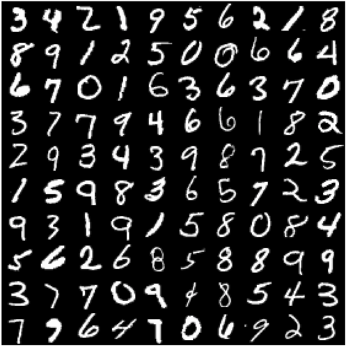
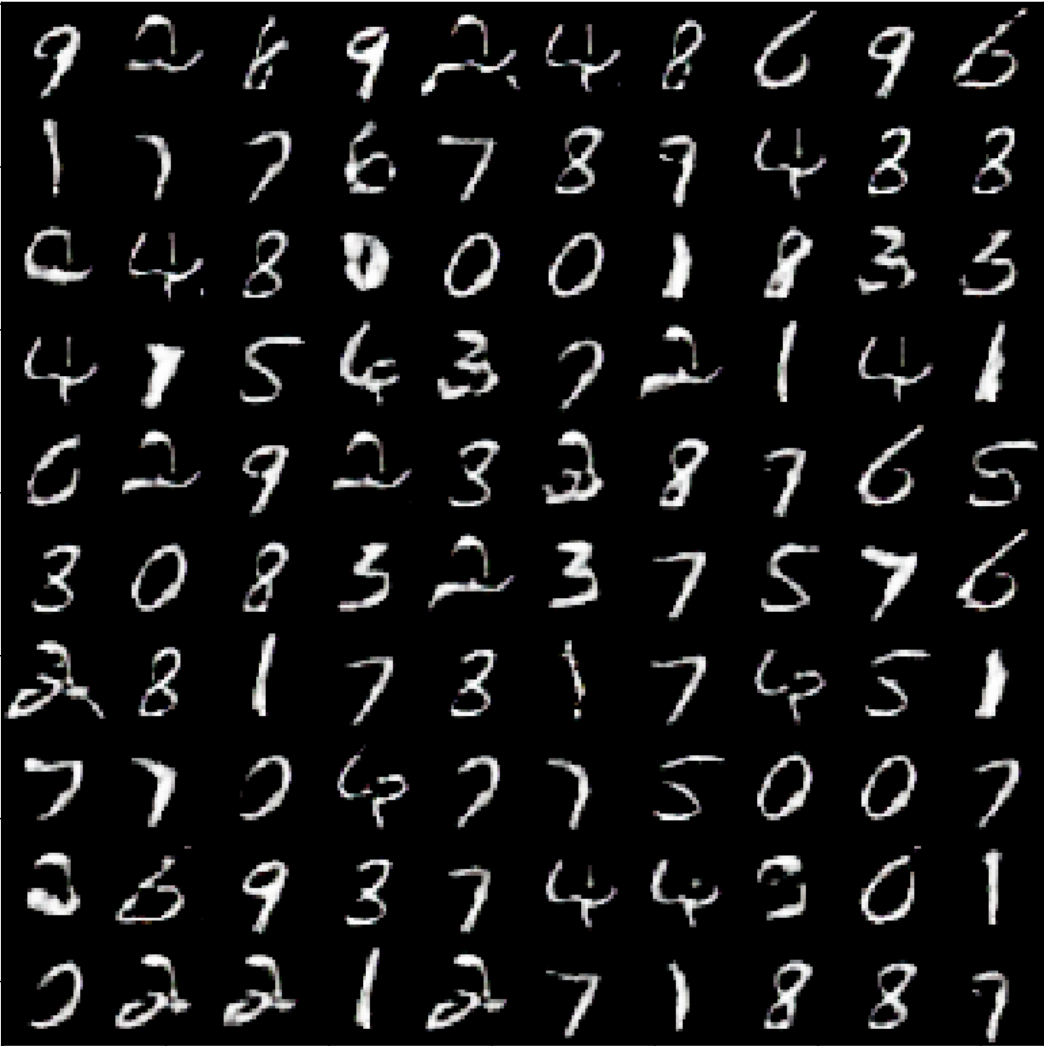
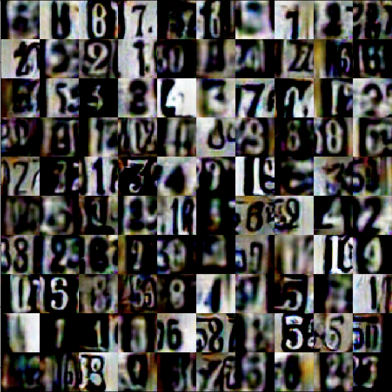
Generated images are shown in Figure 4 for MNIST $\rightarrow$ SVHN and SVHN $\rightarrow$ MNIST. We see that in both tasks the numbers in the generated images are recognizable, but the shapes, styles or colors were changed. This causes them to look different from the original training images, or simply “bad”. This analysis empirically proves that the distribution of the generated images is different from the training data’s, while keeping meaningful features for the network to learn from.

Feature space visualization

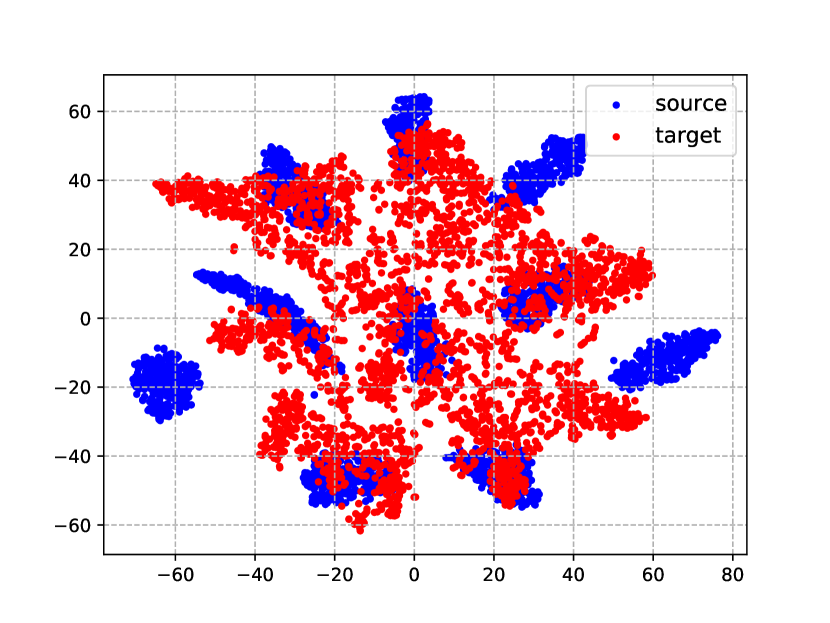
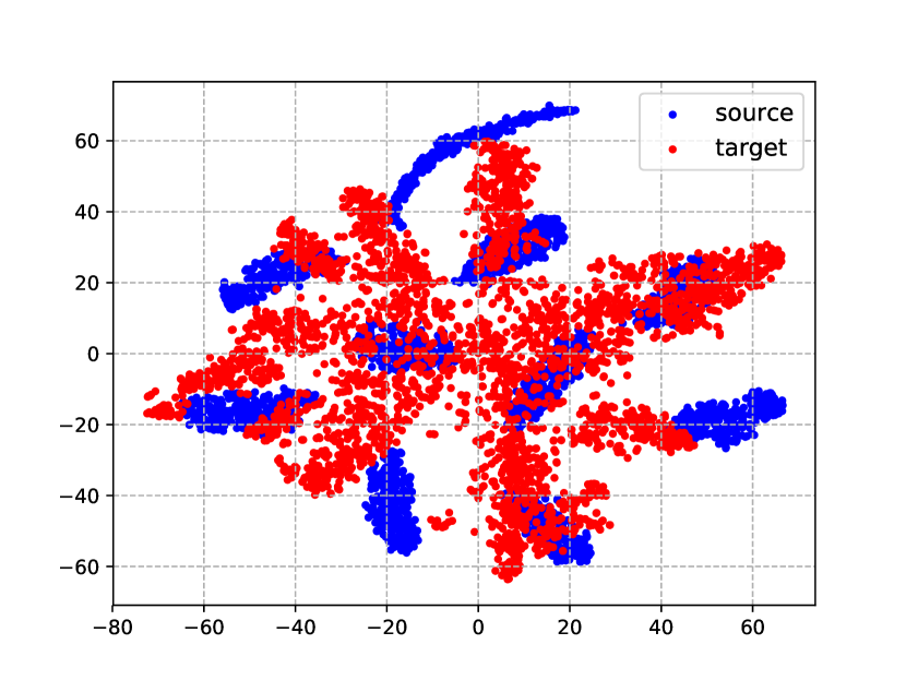
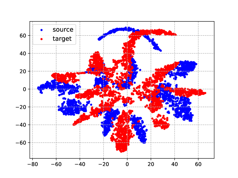
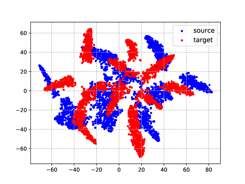
In Figure 5, we compare the T-SNE plots of the last hidden layer of VADA models (Figures 5(a) and 5(c)), and GADA models (Figures 5(b) and  5(d)). We observe that the feature space of GADA is more organized with more separate clusters, compared to those of VADA. GADA increases the distance between clusters, which follows our intuition in the beginning. This results in a much higher accuracy (83.6% compared to 70.6%). When integrated with DIRT-T [21], our performance becomes boosted even further from 83.6% to 90%. This experiment shows the power of GADA, when integrated with other methods, which proves the generic characteristic of our module.

Table 2: Accuracy on test set of the task MNIST $\rightarrow$ SVHN for ablation analysis.

$\pazocal{L}_{c}$	$\pazocal{L}_{d}$	$\pazocal{L}_{e}$	$\pazocal{L}_{v}$	$\pazocal{L}_{u}$	MNIST $\rightarrow$ SVHN
✓	✓				66.3
✓	✓	✓			68.1
✓	✓		✓		69.9
✓	✓			✓	78.7
✓	✓	✓	✓		70.6
✓	✓	✓	✓	✓	83.6

Ablation study

In order to understand the effects of each of loss functions in our algorithm on the accuracy, we perform an extensive ablation study by turning the losses on and off. We test the loss functions on the challenging adaptation task MNIST $\rightarrow$ SVHN. Instance normalization is applied to all the cases in this analysis for fair comparison. The ablation results are given in Table 2. The first row, where only $\pazocal{L}_{c}$ and $\pazocal{L}_{d}$ are used, turns out to be the result for our implementation of DANN [7]. The next three lines show that adding one of $\pazocal{L}_{e}$, $\pazocal{L}_{v}$, or $\pazocal{L}_{u}$ into DANN improves the performance in a stable manner. Among the three, $\pazocal{L}_{u}$ provides the highest improvement ($78.7\%$ compared to $68.1\%$ and $69.9\%$). This improvement indicates that our module could be easily integrated with other methods for higher performance. We merge both $\pazocal{L}_{e}$ and $\pazocal{L}_{v}$ into DANN to have our implementation of VADA [21], which yields better performance than when only one of them is integrated, as expected, though the performance gain is still less than that of solely $\pazocal{L}_{u}$. The best result is achieved when we add $\pazocal{L}_{u}$ into VADA, which creates an improvement of $13\%$ in terms of accuracy and surpasses the state-of-the-art result in CoDA [11]. This experiment, again, shows the power of our module when integrated with other methods.

Confusion matrix

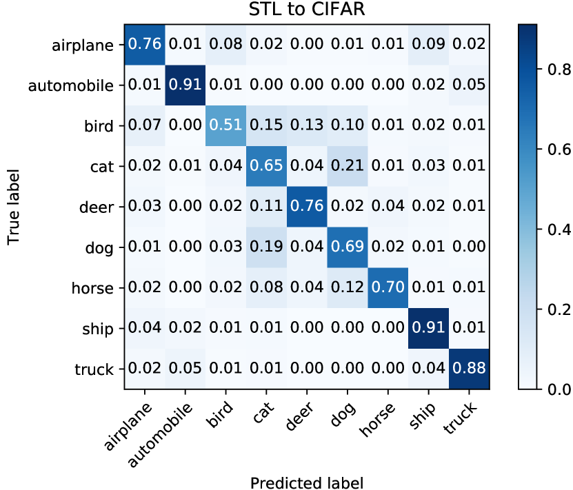
In Figure 6, we present a confusion matrix that shows the prediction accuracy for each of the nine different classes in the task STL-10 $\rightarrow$ CIFAR-10. We observe that our model works very well with several classes, such as ‘automobile,’ ‘ship,’ and ‘truck,’ each of them achieves accuracy of approximately 90%. The class that degrades our performance most is ‘bird’ with only 51% of accuracy. Our model misclassifies the bird images as ‘cat’, ‘deer’, and ‘dog’. We suspect that it is because of the noisy learning in the beginning of the training. The number of labels we have for the classification task is small, which incorrectly moves samples to the wrong clusters.

Figure 6: Confusion matrix for STL-10 $\rightarrow$ CIFAR-10.

5 Conclusion

We proposed the Generative Adversarial Domain Adaptation (GADA) algorithm, which significantly improves the discriminative feature extraction process by injecting an extra class and training with generated samples. The loss functions we proposed have the effects of separating the real target clusters, therby helping the classifier easily find low-density areas to put the decision boundary into. Through extensive experiments on different standard datasets, we showed the effectiveness of our method, and outperformed the other state-of-the-art algorithms in many cases, especially on the highly challenging adaptation task MNIST $\rightarrow$ SVHN. In addition, our module is proved to be extremely effective when integrated into other methods.

 
Supplementary Materials
 

S1 Network architectures

In Table S1, we present the network architectures of the main classifier, which has a small version for digit datasets (MNIST, SVHN, MNIST-M, SynthDigits) and a large one for object datasets (CIFAR-10 and STL-10). Domain discriminator architecture is in Table S2, which is the same for both small and large classifiers. Generator architecture used in the end-to-end training scheme for digit datasets is presented in Table S3. Recall that for the object datasets, we perform a pretraining stage to train the generator. This stage uses a generator architecture in Table S4 and a discriminator architecture in Table S5. The architecture and training scheme in this pretraining stage partially follows DCGAN [16].

Please note in the task SVHN $\rightarrow$ MNIST, the input features to the domain discriminator $D$ is chosen to be the last layer of the classifier $f$ (Layer 15, before softmax), and the feature layer chosen to calculate the mean for generator training is Layer 13. For all other tasks, input features to the domain discriminator $D$ is from Layer 13, and the feature mean for generator training is calculated using output from Layer 14.

Table S1: Network architecture for the main classifier $f$. ‘SAME’ and ‘VALID’ indicate the padding scheme used in each convolutional layer. Batch normalization is applied before activation of all convolutional and dense layers. Leaky ReLU parameter $\alpha$ is set to 0.1. The use of the additive Gaussian noise is empirically proved to improve the performance.

Layer Index	SMALL NETWORK	LARGE NETWORK
0	$32\times 32\times 3$ input images
1	Instance Normalization (optional)
2	$32\times 3\times 3$ Conv (SAME), lReLU	$96\times 3\times 3$ Conv (SAME), lReLU
3	$32\times 3\times 3$ Conv (SAME), lReLU	$96\times 3\times 3$ Conv (SAME), lReLU
4	$32\times 5\times 5$ Conv (VALID), lReLU	$96\times 5\times 5$ Conv (VALID), lReLU
5	$2\times 2$ max-pooling, stride 2
6	Dropout, $p=0.5$
7	Gaussian noise, $\sigma=1$
8	$64\times 3\times 3$ Conv (SAME), lReLU	$192\times 5\times 5$ Conv (SAME), lReLU
9	$64\times 3\times 3$ Conv (SAME), lReLU	$192\times 5\times 5$ Conv (SAME), lReLU
10	$64\times 5\times 5$ Conv (VALID), lReLU	$192\times 5\times 5$ Conv (VALID), lReLU
11	$2\times 2$ max-pooling, stride 2
12	Dropout, $p=0.5$
13	Gaussian noise, $\sigma=1$
14	Dense 500, lReLU	Dense 2048, lReLU
15	Dense output, softmax

Table S2: Network architecture for the domain discriminator $D$. Input features are the output of Layer 15 before softmax (in SVHN $\rightarrow$ MNIST) or the output of Layer 13 (in all other tasks) from the main classifier $f$.

Layer Index	Domain Discriminator
0	Input features
1	Dense 500, ReLU
2	Dense 100, ReLU
3	Dense 1, sigmoid

Table S3: Generator architecture used for the small classifier. All transposed convolutional layers use the ‘SAME’ padding scheme. Batch normalization is applied before activation of all transposed convolutional and dense layers, except for the output layer. Leaky ReLU parameter $\alpha$ is set to 0.1.

Layer Index	Discriminator
0	Input noise vector of length $100$
1	Dense 8192, reshape to $512\times 4\times 4$, lRELU
2	$256\times 3\times 3$ Transposed Conv, stride 2, lRELU
3	$128\times 3\times 3$ Transposed Conv, stride 2, lRELU
4	$3\times 3\times 3$ Transposed Conv, stride 2, tanh

Table S4: Generator architecture used in pretraining and then for the large classifier. All transposed convolutional layers use the ‘SAME’ padding scheme. Batch normalization is applied before activation of all transposed convolutional and dense layers, except for the output layer.

Layer Index	Discriminator
0	Input noise vector of length $100$
1	Dense 2048, reshape to $512\times 2\times 2$, ReLU
2	$256\times 5\times 5$ Transposed Conv, stride 2, RELU
3	$128\times 5\times 5$ Transposed Conv, stride 2, RELU
4	$64\times 5\times 5$ Transposed Conv, stride 2, RELU
5	$3\times 5\times 5$ Transposed Conv, stride 2, tanh

Table S5: Network architecture for the discriminator used in GAN pretraining. All convolutional layers use the ‘SAME’ padding scheme. Batch normalization is applied before activation of all transposed convolutional and dense layers, except for the first convolutional layer and the output layer. Leaky ReLU parameter $\alpha$ is set to 0.1.

Layer Index	Discriminator
0	$32\times 32\times 3$ input images
1	$64\times 5\times 5$ Conv, stride 2, lRELU
2	$128\times 5\times 5$ Conv, stride 2, lRELU
3	$256\times 5\times 5$ Conv, stride 2, lRELU
4	$512\times 5\times 5$ Conv, stride 2, lRELU
5	Dense 1, sigmoid

S2 Hyperparameters

In all experiments, we restrict the hyperparameter search to $\lambda_{d}=\{10^{-2},0\}$, $\lambda_{s}=\{0,1\}$, $\lambda_{t}=\{10^{-1},10^{-2}\}$, $\lambda_{u}=\{10^{-1},1\}$, and $\text{lr}=\{2\times 10^{-4},10^{-3}\}$. The set of hyperparameters which work the best for each task is given in the Table S6. We observe that $\lambda_{u}=1$ works constantly well on all the cases, and changing this value to $10^{-1}$ does not affect the performance much. Note that $\pazocal{L}_{e}$ and $\pazocal{L}_{v}$ are not used in the tasks SVHN $\rightarrow$ MNIST and CIFAR-10 $\rightarrow$ STL-10 $\left(\lambda_{s}=\lambda_{t}=0\right)$. $\lambda_{d}$ is set to $0$ in the tasks CIFAR-10 $\leftrightarrow$ STL-10 following the prior belief in [21]. $\lambda_{s}$ is set to $0$ in the task STL-10 $\rightarrow$ CIFAR-10 because the number of source samples in this case (STL-10 images) is very small, which is unreliable to learn from. All trainings use Adam Optimizer with $\beta_{1}=0.5$ and $\beta_{2}=0.999$.

Table S6: Hyperparameters used for each task.

Task	$\lambda_{d}$	$\lambda_{s}$	$\lambda_{t}$	$\lambda_{u}$	lr
MNIST $\rightarrow$ SVHN	$10^{-2}$	1	$10^{-2}$	1	$2\times 10^{-4}$
SVHN $\rightarrow$ MNIST	$10^{-2}$	0	0	1	$2\times 10^{-4}$
MNIST $\rightarrow$ MNIST-M	$10^{-2}$	0	$10^{-2}$	1	$2\times 10^{-4}$
SynthDigits $\rightarrow$ SVHN	$10^{-2}$	1	$10^{-2}$	1	$2\times 10^{-4}$
CIFAR-10 $\rightarrow$ STL-10	0	0	0	1	$10^{-3}$
STL-10 $\rightarrow$ CIFAR-10	0	0	$10^{-1}$	1	$10^{-3}$

Note that in both tasks CIFAR-10 $\rightarrow$ STL-10 and STL-10 $\rightarrow$ CIFAR-10, we pretrain the generator before actually doing the main training phase. During the pretraining, we train the generator with a learning rate of $10^{-4}$ and train the discriminator with a learning rate of $10^{-3}$. After that, we use the pretrained generator to train the classifier $f$ for the domain adaptation tasks. During this main training phase, we keep fine-tuning the generator with a small learning rate of $2\times 10^{-5}$. In addition, for the task CIFAR-10 $\rightarrow$ STL-10, we pretrain the generator with only 15 epochs, while for the task STL-10 $\rightarrow$ CIFAR-10, we use 100 epochs. This is due to a large difference between number of samples in STL-10 dataset ($450$ images) compared to that of CIFAR-10 ($45,000$ images).

S3 More on how OOC samples help separate the real clusters

S3.1 Limitations of VADA and DIRT-T

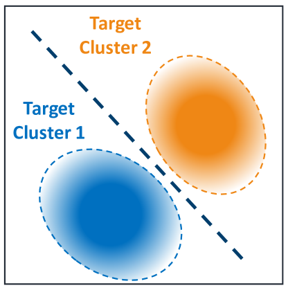
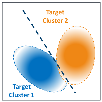
Recall that in VADA and DIRT-T methods [21], the authors tried to move the decision boundaries to low-density areas, with the assumption that the features in the feature space are located into separate clusters, where samples in the same cluster share the same label. However, a perfect scenario in Figure 1(a), where the target clusters are clearly separate so that the decision boundary could go through the low-density area between them, is not guaranteed because the model has no information on the target labels. This perfect scenario could happen with source clusters, where we have excessive information about labels, but not with target clusters. A more realistic scenario is illustrated in Figure 1(b), where the target clusters have a small overlapping region, thereby degrading the performance despite the fact that the decision boundary is passing the low-density area between the two clusters. In our research, the goal is to create larger areas between the target clusters in the feature space so that they are clearly separated. In other words, we want to increase the distance between the target clusters in the feature space.

(a) Perfect Scenario

(b) Real Scenario

Figure S1: Problem of VADA and DIRT-T [21]. The authors assume a perfect scenario as in Figure 1(a), while the scenario that will probably happen is in Figure 1(b).

S3.2 How OOC samples help

Figure S2: Intuition of how OOC samples help in the learning process. Suppose in the feature space extracted by a neural network, there are two overlapping feature clusters of real data and several green feature points of generated samples ($1^{\text{st}}$ figure). All the generated samples should belong to the same fake $\text{(K+1)}^{\text{th}}$ class, so they will be moved closer to each other into a same new cluster ($2^{\text{nd}}$ figure). The two real-class-feature clusters belong to the real classes, so they should not overlap with the features of the generated samples. Therefore, they will be moved away from the position of generated-sample features in the middle ($3^{\text{rd}}$ figure). After all mentioned learning steps, the feature space ends up with the fake cluster being placed in the middle of the two real clusters ($4^{\text{th}}$ figure).

In our model, the classifier $f$ must distinguish between the real and fake samples in order to make the real clusters more separated, thereby improving the performance. An illustration is given in Figure S2 to explain this statement. In this figure, we see that the feature space ends up with the fake cluster being placed in the middle of the two real clusters. This scenario increases the distance between the real clusters, thereby achieving the ultimate goal.

One might argue that the fake cluster could be placed far away from the real clusters. However, this situation should not happen given that the generated samples have features similar to the ones of real data. For example, consider a generator trying to generate numbers from the MNIST dataset. Suppose in the feature space, real clusters of number $1$ and of number $7$ are placed near each other because of their similar shape. Weird-shape numbers $1$ and $7$ are generated, i.e., they come from a distribution different from the distribution of normal-shape numbers $1$ and $7$ in the training data. These generated numbers are “bad”, but they are still $1$ and $7$, which should be placed near the corresponding clusters in the feature space. On the other hand, these generated samples belong to the same fake cluster. Therefore, they will be moved to a same cluster while staying near the corresponding real clusters, which results in a feature space similar to the $4^{\text{th}}$ figure in Figure S2.

S4 Generated images

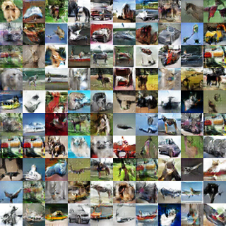
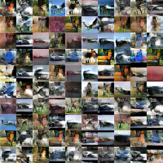
We show some of the generated images on the tasks CIFAR-10 $\rightarrow$ STL-10 and STL-10 $\rightarrow$ CIFAR-10. We could observe that the generated samples on CIFAR-10 in Figure 3(a) have higher quality in terms of variety, compared to STL-10 generated images in Figure 3(b). This is because of a large difference between the numbers of unsupervised training samples given in each task. Number of STL-10 target samples is much lower than that of the CIFAR-10 dataset: $450$ compared to $45,000$ respectively.

(a) Generated CIFAR-10 images

(b) Generated STL-10 images

Figure S3: Generated images on the task 3(a) STL-10 $\rightarrow$ CIFAR-10 and 3(b) CIFAR-10 $\rightarrow$ STL-10.

References

- [1] Dario Amodei, Sundaram Ananthanarayanan, Rishita Anubhai, Jingliang Bai, Eric Battenberg, Carl Case, Jared Casper, Bryan Catanzaro, Qiang Cheng, Guoliang Chen, et al. Deep speech 2: End-to-end speech recognition in english and mandarin. In International conference on machine learning, pages 173–182, 2016.
- [2] Pablo Arbelaez, Michael Maire, Charless Fowlkes, and Jitendra Malik. Contour detection and hierarchical image segmentation. IEEE transactions on pattern analysis and machine intelligence, 33:898–916, 05 2011.
- [3] Konstantinos Bousmalis, Nathan Silberman, David Dohan, Dumitru Erhan, and Dilip Krishnan. Unsupervised pixel-level domain adaptation with generative adversarial networks. In 2017 IEEE Conference on Computer Vision and Pattern Recognition (CVPR), pages 95–104, 2017.
- [4] Konstantinos Bousmalis, George Trigeorgis, Nathan Silberman, Dilip Krishnan, and Dumitru Erhan. Domain separation networks. In Advances in Neural Information Processing Systems, pages 343–351, 2016.
- [5] Zihang Dai, Zhilin Yang, Fan Yang, William W Cohen, and Ruslan R Salakhutdinov. Good semi-supervised learning that requires a bad gan. In Advances in Neural Information Processing Systems 30, pages 6510–6520, 2017.
- [6] Yaroslav Ganin and Victor Lempitsky. Unsupervised domain adaptation by backpropagation. In Proceedings of the 32nd International Conference on Machine Learning, pages 1180–1189, 2015.
- [7] Yaroslav Ganin, Evgeniya Ustinova, Hana Ajakan, Pascal Germain, Hugo Larochelle, François Laviolette, Mario Marchand, and Victor Lempitsky. Domain-adversarial training of neural networks. The Journal of Machine Learning Research, 17(1):2096–2030, 2016.
- [8] Ian Goodfellow, Jean Pouget-Abadie, Mehdi Mirza, Bing Xu, David Warde-Farley, Sherjil Ozair, Aaron Courville, and Yoshua Bengio. Generative adversarial nets. In Advances in neural information processing systems, pages 2672–2680, 2014.
- [9] Kaiming He, Xiangyu Zhang, Shaoqing Ren, and Jian Sun. Deep residual learning for image recognition. In Proceedings of the IEEE conference on computer vision and pattern recognition, pages 770–778, 2016.
- [10] Judy Hoffman, Eric Tzeng, Taesung Park, Jun-Yan Zhu, Phillip Isola, Kate Saenko, Alexei Efros, and Trevor Darrell. CyCADA: Cycle-consistent adversarial domain adaptation. In Proceedings of the 35th International Conference on Machine Learning, pages 1989–1998, 2018.
- [11] Abhishek Kumar, Prasanna Sattigeri, Kahini Wadhawan, Leonid Karlinsky, Rogerio Feris, Bill Freeman, and Gregory Wornell. Co-regularized alignment for unsupervised domain adaptation. In Advances in Neural Information Processing Systems, pages 9345–9356, 2018.
- [12] Mingsheng Long, Yue Cao, Jianmin Wang, and Michael I. Jordan. Learning transferable features with deep adaptation networks. In Proceedings of the 32Nd International Conference on International Conference on Machine Learning - Volume 37, pages 97–105, 2015.
- [13] Mingsheng Long, Han Zhu, Jianmin Wang, and Michael I. Jordan. Deep transfer learning with joint adaptation networks. In Proceedings of the 34th International Conference on Machine Learning - Volume 70, pages 2208–2217, 2017.
- [14] Zak Murez, Soheil Kolouri, David J. Kriegman, Ravi Ramamoorthi, and Kyungnam Kim. Image to image translation for domain adaptation. In 2018 IEEE Conference on Computer Vision and Pattern Recognition (CVPR), pages 4500–4509, 2018.
- [15] Guo-Jun Qi, Liheng Zhang, Hao Hu, Marzieh Edraki, Jingdong Wang, and Xian-Sheng Hua. Global versus localized generative adversarial nets. In The IEEE Conference on Computer Vision and Pattern Recognition (CVPR), 2018.
- [16] Alec Radford, Luke Metz, and Soumith Chintala. Unsupervised representation learning with deep convolutional generative adversarial networks. In International Conference on Learning Representations, 2016.
- [17] Artem Rozantsev, Mathieu Salzmann, and Pascal Fua. Beyond sharing weights for deep domain adaptation. IEEE Transactions on Pattern Analysis and Machine Intelligence, 41:801–814, 2018.
- [18] Kuniaki Saito, Yoshitaka Ushiku, and Tatsuya Harada. Asymmetric tri-training for unsupervised domain adaptation. In Proceedings of the 34th International Conference on Machine Learning, pages 2988–2997, 2017.
- [19] Kuniaki Saito, Kohei Watanabe, Yoshitaka Ushiku, and Tatsuya Harada. Maximum classifier discrepancy for unsupervised domain adaptation. In 2018 IEEE Conference on Computer Vision and Pattern Recognition (CVPR), pages 3723–3732, 2018.
- [20] Tim Salimans, Ian Goodfellow, Wojciech Zaremba, Vicki Cheung, Alec Radford, Xi Chen, and Xi Chen. Improved techniques for training gans. In Advances in Neural Information Processing Systems 29, pages 2234–2242, 2016.
- [21] Rui Shu, Hung Bui, Hirokazu Narui, and Stefano Ermon. A DIRT-t approach to unsupervised domain adaptation. In International Conference on Learning Representations, 2018.
- [22] Baochen Sun and Kate Saenko. Deep coral: Correlation alignment for deep domain adaptation. In Computer Vision – ECCV 2016 Workshops, pages 443–450, 2016.
- [23] Eric Tzeng, Judy Hoffman, Kate Saenko, and Trevor Darrell. Adversarial discriminative domain adaptation. In IEEE Conference on Computer Vision and Pattern Recognition, CVPR 2017, pages 2962–2971, 2017.
- [24] Eric Tzeng, Judy Hoffman, Ning Zhang, Kate Saenko, and Trevor Darrell. Deep domain confusion: Maximizing for domain invariance. CoRR, abs/1412.3474, 2014.
- [25] Kai-Ya Wei and Chiou-Ting Hsu. Generative adversarial guided learning for domain adaptation. In British Machine Vision Conference (BMVC), 2018.
- [26] Shaoan Xie, Zibin Zheng, Liang Chen, and Chuan Chen. Learning semantic representations for unsupervised domain adaptation. In Proceedings of the 35th International Conference on Machine Learning, pages 5423–5432, 2018.
- [27] Werner Zellinger, Thomas Grubinger, Edwin Lughofer, Thomas Natschläger, and Susanne Saminger-Platz. Central moment discrepancy (cmd) for domain-invariant representation learning. In International Conference on Learning Representations, 2017.
- [28] Jun-Yan Zhu, Taesung Park, Phillip Isola, and Alexei A. Efros. Unpaired image-to-image translation using cycle-consistent adversarial networks. In IEEE International Conference on Computer Vision, ICCV 2017, Venice, Italy, October 22-29, 2017, pages 2242–2251, 2017.