Statistical Inversion Using Sparsity and Total Variation Prior And Monte Carlo Sampling Method For Diffuse Optical Tomography

Abstract

In this paper, we formulate the reconstruction problem in diffuse optical tomography (DOT) in a statistical setting for determining the optical parameters, scattering and absorption, from boundary photon density measurements. A special kind of adaptive Metropolis algorithm for the reconstruction procedure using sparsity and total variation prior is presented. Finally, a simulation study of this technique with different regularization functions and its comparison to the deterministic Iteratively Regularized Gauss Newton method shows the effectiveness and stability of the method.

1 Introduction

Diffuse Optical Tomography (DOT) is an imaging modality for probing highly scattering media by using low-energy visible (wavelength from 380nm to 750 nm) or near-infrared light (wavelength from 700 to 1200 nm). Light penetrates the media and interacts with its tissue. The predominant effects are absorption and scattering [27, 12, 17, 31]. The widely accepted photon transport model is the Radiative Transfer Equation (RTE) [14, 34], an integro-differential equation for the radiance, involving spatially varying diffusion and absorption parameters, which are a priori unknown. Hence the inverse problem consists of reconstructing an image of the optical properties (absorption and diffusion coefficients) of the tissue from measurements of some function of the photon density on the boundary. The optical properties will vary significantly between background tissue and potential tumors, making DOT an attractive imaging technique. Further, the scattering and absorption parameters are functional information, which are not acquired by standard x-ray attenuation type techniques, that can give information such as hemoglobin, water content, and lipid concentration [7].
In practice, a low order diffusion approximation to the RTE is often adopted which is the standard model in DOT. The approximation is a parabolic and an elliptic differential equation in the time-dependent case and in the steady-state case or the frequency domain, respectively [3, 2]. Most existing computational methods for the forward problems as well as inverse problems of photon migration in biological tissues are based on the approximation because of its simplicity compared to the full blown radiative transfer equation [13, 32]. It is well known that the DOT inverse problem is exponentially ill-posed [3, 48]. Image reconstruction in DOT is highly nonlinear and unstable [4, 44]. In fact, DOT is an excellent example of a severely ill-posed inverse problem and is getting more and more attention [4, 27, 44]. The DOT inverse problem also includes electrical impedance tomography (EIT) as a special case [8]. There is great interest in understanding the inverse problem in DOT due to the huge impact in potential applications such as medical imaging for example neo-natal brain imaging, detection of breast cancer, and osteoarthritis detection. DOT is a preferred modality because of its low cost, non-invasiveness, and safe use of mainly near infrared (compared to x-ray) light radiation [27, 38]. In order to solve an inverse problem using the elliptic partial differential equation (PDE) model such as in DOT, many computational issues must be considered such as model error, nonlinearity, linearization via adjoint, uniqueness/non-uniquness, ill-posedness, regularization etc. (see [44, 49, 55, 64, 43, 45, 9, 63, 33, 36, 39, 41, 54, 37, 35, 42, 56] for details).
In order to overcome the main difficulties of the ill-posed inverse problem in DOT, regularization is required to find a reasonable solution for this problem. There exists vast literature on how to regularize a nonlinear ill-posed problem such as DOT. For example, Tikhonov and iterated soft-shrinkage regularization methods for nonlinear inverse medium scattering problems [46], a nonlinear ART or Kaczmarz method [49], a conjugate gradient type method [52], variations/hybrid of Newton’s method [49, 50], diffusion-backdiffusion algorithms [5, 49], total variation algorithms [16] such as using level sets [19, 20, 21], iteratively regularized Gauss-Newton [57] etc. have been investigated for DOT . However the reconstruction results are still not satisfactory for DOT.
In recent years, statistical methods and regularizations [40, 60, 61, 58, 1] have been studied for reconstructing the EIT problem. In this paper we extend some of the results for EIT to DOT. That is, we formulate the DOT problem in terms of a posterior density, introduce statistical regularization methods and finally use the Markov Chain Monte Carlo to find a point estimate for the absorption and diffusion coefficients from boundary measurements. We note that classical algorithms such as the Metropolis Hastings [47, 30, 15] or the Gibbs Sample [26] are not performing well for this particular problem in our experience. Hence, we are using a special kind adaptive Metropolis algorithm [60] to obtain a proper reconstruction of the absorption and diffusion coefficients in a suitable about of time. There is a vast amount of statistical literature on adaptive Metropolis algorithms such as [29, 28, 23, 24].
This paper is organized in the following way: In section 2 the analytical forward problem of DOT is described. In section 3, the Fréchet differentiability of the DOT forward operator is discussed, which is used in section 4 for the brief description of the iteratively regularized Gauss-Newton (IRGN) method used as comparison to the main result of this paper. Proof of the convergency of IRGN is presented in section 5. In section 6, the in statistical inverse problem is is formulated, mainly describing the posterior density, different regularization functions, the Markov Chain Monte Carlo method, and a pilot adaptive Metropolis algorithm. In section 7, simulation from noisy measurements are presented to show the effectiveness and stability of the method and compare it to the classical Newton method. Finally in section 8, we resume the paper presenting final concussions.

2 The Forward Problem

To model light traveling through tissue, the scattering and absorption qualities of the medium are required. Specifically the reduced scattering coefficient $\mu_{s}^{\prime}$ and absorption coefficient $\mu_{a}$ from the RTE, which models this type of physical system, are needed. Approximating with the frequency domain diffusion approximation to the RTE, the result is a fairly simple model for optical tomography:

$$-\nabla\cdot\left(D\nabla u\right)+(\mu+ik)u=h\quad\mbox{ in }\Omega$$

where $D=\frac{1}{3(\mu_{a}+\mu_{s}^{\prime})}$ represents the diffusion coefficient, $\mu=\mu_{a}$ represents the absorption coefficient. $u$ is the photon density, $h$ is the interior source, and $k=\omega/c$ for $\omega$ the frequency of the source and $c$ the velocity of light in the medium. The solution $u$ represents the photon density. The model was derived in detail in [3]. With this DOT model in hand, we have the Neumann

$$-\nabla\cdot\left(D\nabla u\right)+(\mu+ik)u =h,\quad\mbox{ in }\Omega$$

$$D\frac{\partial u}{\partial\nu} =f,\quad\mbox{on }\partial\Omega$$

forward problem. The solutions to this problem is referred to as $F_{N}^{(k,q)}(h,g)$ where $q=(D,\mu)$ represents the parameters. It is assumed that $f\in H^{-1/2}(\partial\Omega)$ and $g\in H^{1/2}(\partial\Omega)$. Further, $\gamma_{0}:H^{1}(\Omega)\rightarrow H^{1/2}(\partial\Omega)$ denotes the Dirichlet trace map. For the purposes of this manuscript, the homogeneous case is considered with $h=0$.

To simplify the solution space, it is assumed that $D,\mu\in L^{\infty}(\Omega)$, $0<D_{0}<D(x)<D_{1}$, and $0<\mu(x)<\mu_{1}<\infty$ for positive real constants $D_{0},D_{1}$ and $\mu_{1}$. Then the resulting photon density $u$ belongs to $H^{1}(\Omega)$. The well-posedness of these problems has been shown in [18]. In [50], the authors shows the uniqueness of the forward DOT operator.

3 Fréchet differentiability of the DOT operator

The inverse problem of the DOT problem is to estimate the diffusion ($D$) and the absorption ($\mu$) coefficient for a source function $f$. We solve the inverse problem using iteratively regularized Gauss-Newton (IRGN) method, for which a Fréchet differentiablity of the map $\gamma_{0}{F_{N}}^{(k,q^{\dagger})}(0,f)$ is a necessary tool. Recall that Fréchet differentiability of $\gamma_{0}{F_{N}}^{(k,q^{\dagger})}(0,f)$ is defined as

$$\lim_{||\eta||_{\infty}\to 0} \frac{||\gamma_{0}{F_{N}}^{(k,q^{\dagger})}(q+\eta:0,f)-\gamma_{0}{F_{N}}^{(k,q^{\dagger})}(q:0,f)-\gamma_{0}{F^{\prime}_{N}}^{(k,q^{\dagger})}(q:0,f)\eta||}{||\eta||_{\infty}}$$

$$=0$$

Theorem 1.

Suppose $q_{1}=(D_{1},\mu_{1}),q_{2}=(D_{2},\mu_{2})$ are two pairs of real-valued $L_{\infty}(\Omega)$ functions satisfying,

$$0<m_{D}\leq D_{1,2}(x)\leq M_{D},\quad 0\leq\mu_{1,2}(x)\leq M_{\mu},\mbox{ for some }m_{D},M_{D},M_{\mu}>0$$

then there exists a constant $C$, such that,

$$||\gamma_{0}{F_{N}}^{(k,q^{\dagger})}(q_{2}:0,f)-\gamma_{0}{F_{N}}^{(k,q^{\dagger})}(q_{1}:0,f)- \gamma_{0}{F^{\prime}_{N}}^{(k,q^{\dagger})}(q_{1}:0,f)\eta||$$

$$\leq C||\eta||_{\infty}^{2}$$ (1)

where $\eta=q_{2}-q_{1}$. In particular, $\gamma_{0}{F^{\prime}_{N}}^{(k,q^{\dagger})}(q_{1}:0,f)$ is the Fréchet derivative of $\gamma_{0}{F_{N}}^{(k,q^{\dagger})}(0,f)$ with respect to $q$ at $q_{1}$.

Proof.

See [50]. ∎

4 Inverse Problem

The Neumann-to-Dirichlet map $\gamma_{0}F_{N}^{(k,q^{\dagger})}(0,f)$ amounts to conducting the forward problem experiment over the true parameters $q^{\dagger}$. Because of imprecise measurements, the boundary information used is denoted

$$g^{\gamma}=\gamma_{0}F_{N}^{(k,q^{\dagger})}(0,f)+\xi$$

where $\xi$ represents the noise. The forward problem uses $q$ to find the boundary data associated with a given source $f$. The inverse problem is to estimate the parameter $q=(D,\mu)$, for a set of source functions. Since the forward problem is well-posed, it is sufficient to consider $q\in\{L_{\infty}\times L_{\infty}:0<m_{D}\leq D\leq M_{D},0<\mu<\infty\}$. However, in order to establish the uniqueness of the solution to the inverse problem, we consider $q\in\{H_{2}(\Omega)\times L_{2}(\Omega):0<m_{D}\leq D\leq M_{D},0<\mu<\infty\}$.

Theorem 2.

A solution $q$ to the DOT inverse problem exists and is unique. That is given the measurements on the boundary, we can reconstruct a unique spatial map for the parameter $q$.

Proof.

The proof of this theorem is well-established in the literature, see [62]. ∎

Since the inverse problem is severely ill-posed, in order to recover $q$, we minimize the following cost functional from the finite set of measurements.

$$J_{\gamma}(q)=||\gamma_{0}F_{N}^{(k,q)}(0,f)-g^{\gamma}||_{2}^{2}$$

where $g^{\gamma}$ approximates the exact data $g$ with the accuracy $\xi$, i.e.,

$$||g-g^{\gamma}||<\xi.$$ (2)

However, regularization is needed to improve the ill-posed problem and instead, we minimize,

$$J_{\gamma}(\alpha,q)=||\gamma_{0}F_{N}^{(k,q)}(0,f)-g^{\gamma}||_{2}^{2}+\alpha R(q-q^{*})$$

where $\alpha$ is the regularization parameter, $R(\cdot)$ is the regularization term and $q^{*}$ is the known background.
The regularization function is represented by a norm for most analytical methods. In this paper we used one of the most successful methods for solving the ill-conditioned problem, $R_{\ell_{2}}$ known as Tikhonov regularization. The cost functional from Tikhonov regularization is

$$J_{\gamma}(\alpha,q)=\frac{1}{2}||\gamma_{0}F_{N}^{(k,q)}(0,f)-g^{\gamma}||_{2}^{2}+\frac{\alpha}{2}||\nabla q||_{2}^{2}$$ (3)

There are several iterative approaches to minimize (3). In this paper, we used a modified iteratively regularized Gauss-Newton (IRGN) method for the minimization.
Suppose $\alpha_{k}$ is some sequence of regularizing parameters satisfying the conditions

$$\alpha_{k}\geq\alpha_{k+1}>0,\quad\sup_{k\in\mathbb{N}\cup\{0\}}\frac{\alpha_{k}}{\alpha_{k+1}}=\hat{d}<\infty,\quad\lim_{k\to\infty}\alpha_{k}=0.$$ (4)

Let the unique global minimum of (3) be denoted by $\tilde{q}$. Assume $\tilde{\gamma}$ satisfies the invertibility conditions and the conditions for $F$ as described in [57]. Then, the unique global minimum of (3) is explicitly given by

$$\tilde{q}= q_{k}-(\gamma_{0}F^{\prime}(q_{k})^{T}\gamma_{0}F^{\prime}(q_{k})+\alpha_{k}\triangle_{k}q)^{-1}$$

$$\{\gamma_{0}F^{\prime}(q_{k})^{T}(\gamma_{0}F(q_{k})-g^{\gamma})+\alpha_{k}\triangle_{k}q\}$$ (5)

where $q_{k}$ is the $k$-th approximation to $q$ and $\gamma_{0}F^{\prime}(q_{k})$ is the Jacobian matrix at the $k$-th iteration. The term $\triangle_{k}$ is the discrete Laplacian operator.The above algorithm is generalized further using a line search procedure, as discussed in [57], by introducing a variable step size, $s_{k}$, such that

$$0<s<s_{k}\leq 1.$$ (6)

The modified IRGN algorithm is then

$$q_{k+1}= q_{k}-s_{k}(\gamma_{0}F^{\prime}(q_{k})^{T}\gamma_{0}F^{\prime}(q_{k})+\alpha_{k}\triangle_{k}q_{k})^{-1}$$

$$\{\gamma_{0}F^{\prime}(q_{k})^{T}(\gamma_{0}F(q_{k})-g^{\gamma})+\alpha_{k}\triangle_{k}q_{k})\}.$$ (7)

Due to the inexact nature of $g^{\gamma}$, we adopt a stopping rule from [6] to terminate the iterations at the first index $\mathcal{K}=\mathcal{K}(\delta)$, such that

$$||\gamma_{0}F(q_{\mathcal{K}})-g^{\gamma}||^{2}\leq\rho\xi<||\gamma_{0}F(q_{k})-g^{\gamma}||^{2},\quad 0\leq k\leq\mathcal{K},\quad\rho>1.$$ (8)

The line search parameter $s_{k}$ is chosen to minimize the scalar objective function

$$\Phi(s)=J(q_{k}+sp_{k})$$ (9)

where $p_{k}$ is the search direction, which solves

$$(\gamma_{0}F^{\prime}(q_{k})^{T}\gamma_{0}F^{\prime}(q_{k})+\alpha_{k}\triangle_{k}q_{k})p_{k}=-\gamma_{0}F^{\prime}(q_{k})^{T}(\gamma_{0}F(q_{k})-g^{\gamma})+\alpha_{k}\triangle_{k}q_{k})$$ (10)

This step is accomplished through a backtracking strategy until either one of the strong Wolfe conditions,

$$J(q_{k}+sp_{k})\leq J(q_{k})+\gamma_{1}s\nabla J(q_{k})^{T}p_{k}$$ (11)

$$|\nabla J(q_{k}+sp_{k})^{T}p_{k}|\leq|\gamma_{2}\nabla J(q_{k})^{T}p_{k}|.$$ (12)

is satisfied [51], or the maximum number of backtracking steps has been reached. We use the theoretically derived values of $\gamma_{1}=0.0001$ and $\gamma_{2}=0.9$, derived in [51]. The basic convergence result for the IRGN algorithm (5) combined with the stopping rule (8) is established by the theorem provided in the next section.

5 Convergence of IRGN

Assume that $F$ is a nonlinear operator acts on the Hilbert spaces $(H,H_{1})$, $F:D(F)\subset H\to H_{1}$, and $F$ is Fréchet differentiable in $D(F)$. We consider minimizing the functional

$$J(q)=||F(q)-g_{\delta}||^{2}_{H_{1}}$$ (13)

where $g_{\delta}$ approximates the exact data $g$ with the accuracy $\delta$, i.e.,

$$||g-g_{\delta}||\leq\delta$$ (14)

Our interest is to find an element $\hat{q}\in D(F)$, s.t.

$$||F(\hat{q})-g||_{H_{1}}=\inf_{q\in D(F)}||F(q)-g||_{H_{1}}=0$$ (15)

Consider the following conditions hold

$$||F^{\prime}(q_{1})|| \leq M_{1},\quad\mbox{ for any }q_{1}\in B_{\eta}(\hat{q})$$ (16)

$$||F^{\prime}(q_{1})-F^{\prime}(q_{2})|| \leq M_{2}||q_{1}-q_{2}||,\mbox{ for any }q_{1},q_{2}\in B_{\eta}(\hat{q})$$ (17)

where $B_{\eta}(\hat{q})=\{q\in H:||q-\hat{q}||\leq\eta\}\subset D(F)$. The convergence analysis of IRGN is done under the source condition

$$L^{*}L(\hat{q}-q)=F^{\prime*}(\hat{q})S,\quad S=\{v\in H:||v||\leq\varepsilon\}$$ (18)

and by the following theorem.

Theorem 3.

Assume that
(1) $F$ satisfies (16) and (17) with $\eta=l\sqrt{\tau_{0}}$, conditions (14) and (15) holds.
(2) The regularization sequence $\{\alpha_{k}\}$ and the step size sequence $\{s_{k}\}$ are chosen according to (4) and (6), respectively.
(3) Source condition (18) is satisfied.
(4) The linear operator $L^{*}L$ is surjective and there is a constant $m>0$ such that

$$\langle L^{*}Lh,h\rangle\geq m||h||^{2},\quad\mbox{ for any }h\in H$$ (19)

(5) Constants defining $F$ and the iteration are constrained by

$$\frac{M_{2}\varepsilon}{m}+\frac{d-1}{d\alpha}+\sqrt{\frac{\varepsilon}{m}\left(\frac{M_{2}}{2}+\frac{M_{1}^{2}}{(\sqrt{\rho}-1)^{2}}\right)}\leq 1$$ (20)

$$\frac{||q_{0}-\hat{q}||}{\sqrt{\alpha_{0}}}\leq\frac{\varepsilon}{\sqrt{m}\left(1-\frac{M_{2}\varepsilon}{m}-\frac{d-1}{d\alpha}\right)}=l$$ (21)

Then,
(1) For iterations (5)

$$\frac{||q_{k}-\hat{q}||}{\sqrt{\alpha_{k}}}\leq l,\quad k=0,1,...,\mathcal{K}(\delta)$$ (22)

(2) The sequence $\{\mathcal{K}(\delta)\}$ is admissible, i.e.

$$\lim_{\delta\to 0}||q_{\mathcal{K}(\delta)}-z||=0,$$ (23)

$z$ is $\arg\inf_{q\in D(F)}||F(q)-g||_{H_{1}}$.

Proof.

See [57], for the details of the proof. ∎

6 Statistical Inverse Problem

Modeling the forward problem uses knowledge of the absorption, $\mu_{a}$, and the scattering, $\mu_{s}^{\prime}$ parameters to find the boundary data associated with a given source. The inverse problem instead uses knowledge of the source and boundary data, and seeks to uncover the absorption and scattering parameters. Our stated goal is to recover $\mu_{a}$, and $\mu_{s}^{\prime}$. However, considering the proposed model for optical tomography in this document, this is equivalent to the recovery of $q=(D,\mu)$. These parameters have a high contrast between a tumor and the background and consequently acquiring an accurate representation of these parameters will allow for the detection of homogeneity’s.

Because, we can not directly calculate the inverse to the forward problem, the inverse problem can be represented as a minimization problem of a cost functional. One possibility is using the standard least squares fitting as discrepancy functional,

$$J(q)=\frac{1}{2}\left\|\gamma_{0}F_{N}^{(k,q)}(0,f)-g^{\gamma}\right\|^{2}_{L_{2}(\partial\Omega)}$$

for a source $f$ and measurement $g^{\gamma}$. However, minimizing $J(q)$ won’t result in a proper reconstruction due to the high ill-posedness of the problem. Hence, typical analytical approaches try to find an estimate $\hat{q}$ of $q$ by solving

$$\hat{q}=argmin_{q}J(q)+\alpha R(q)$$

where $R(q)$ is a regularization function and $\alpha>0$ the regularization parameter. In this section we shall reformulate this minimization problem into finding a Bayes’ estimate from a posterior density.

6.1 The Posterior Density

With a slight abuse of notation we denote $D,\mu,q,g$ as its continuous setting as well as its discrete analogue. Further, let $\epsilon$ be the discrete measurement noise of the measurements $g$. Let $q^{*},D^{*},\mu^{*},\epsilon^{*}$ and $g^{*}$ be the random variables for the deterministic values $q,D,\mu,\epsilon$ and $g$ respectively. Let $D,\mu$ be $n\in\mathbb{N}$ dimensional parameters. Hence, $q$ is a $2n$ dimensional parameter to be recovered. The measurements $g$ and the measurement noise $\epsilon$ are assumed to be both $m\in\mathbb{N}$ dimensional parameters. Let $\Theta(q,\epsilon)$ denote the discrete operator that solves the forward problem on $\partial\Omega$. That is, if the forward problem is well-posed, it follows that $g=\Theta(q,\epsilon)$.

The solution of a statistical inverse problem of the parameter $q$ is generally defined as the posterior density of $q^{*}$ given the measurements $g$ and the measurement noise $\epsilon$, e.i. $\pi_{q^{*}}(q|g,\epsilon)$. The posterior density $\pi_{q^{*}}(q|g,\epsilon)$ shall be derived first. From the statistical point of view it is clear that

$$\pi_{g^{*}}(g|q,\epsilon)=\delta(g-\Theta(q,\epsilon)),$$

where $\delta$ is the Dirac delta function. The Dirac delta function is not a function in a strict sense, however the integral over $\delta(\cdot)$ is in fact a distribution function. The joint density of $q^{*},g^{*}$ and $\epsilon^{*}$ is

$$\pi_{q^{*},g^{*},\epsilon^{*}}(q,g,\epsilon)=\pi_{g^{*}}(g|q,\epsilon)\pi_{q^{*},\epsilon^{*}}(q,\epsilon)=\delta(g-\Theta(q,\epsilon))\pi_{q^{*},\epsilon^{*}}(q,\epsilon).$$

However, the measurement noise $\epsilon$ is a unobservable quantity and should be integrated out of the model. The joint density of $q^{*}$ and $g^{*}$ is obtained by

$$\pi_{q^{*},g^{*}}(q,g)=\int_{\mathbb{R}^{m}}\pi_{q^{*},g^{*},\epsilon^{*}}(q,g,\epsilon)d\epsilon=\int_{\mathbb{R}^{m}}\delta(g-\Theta(q,\epsilon))\pi_{q^{*},\epsilon^{*}}(q,\epsilon)d\epsilon.$$ (24)

In order to solve this integral more assumptions on the measurement noise $\epsilon^{*}$ are required. Assume that the measurement noise $\epsilon^{*}$ is independent from the variable of interest $q^{*}$, i.e. $\pi_{q^{*},\epsilon^{*}}(q,\epsilon)=\pi_{q^{*}}(q)\pi_{\epsilon^{*}}(\epsilon)$, and that the measurement noise is additive, i.e. $g=\Theta(q)+\epsilon$. Now equation (24) can be simplified to

$$\pi_{q^{*},g^{*}}(q,g)=\int_{\mathbb{R}^{m}}\delta(g-\Theta(q)-\epsilon)\pi_{q^{*}}(q)\pi_{\epsilon^{*}}(\epsilon)d\epsilon=\pi_{q^{*}}(q)\pi_{\epsilon^{*}}(g-\Theta(q)).$$

It follows that the posterior density of $q^{*}$ given the measurements $g$ is

$$\pi_{q^{*}}(q|g)=\frac{\pi_{q^{*},g^{*}}(q,g)}{\pi_{g^{*}}(g)}=\frac{\pi_{q^{*}}(q)\pi_{\epsilon^{*}}(g-\Theta(q))}{\int_{\mathbb{R}^{2n}}\pi_{q^{*}}(q)\pi_{\epsilon^{*}}(g-\Theta(q))dq}\propto\pi_{q^{*}}(q)\pi_{\epsilon^{*}}(g-\Theta(q)),$$ (25)

where $\int_{\mathbb{R}^{2n}}\pi_{q^{*}}(q)\pi_{\epsilon^{*}}(g-\Theta(q))dq>0$ is a unknown constant. To obtain a proper defined posterior density the densities of $q^{*}$ and $\epsilon^{*}$ must be specified. Assume that the measurement noise is Gaussian distributed, i.e.

$$\pi_{\epsilon^{*}}(g-\Theta(q))\propto\exp\left[-\frac{1}{2}(g-\Theta(q))^{\prime}C^{-1}(g-\Theta(q))\right].$$

Further, assume that the prior density, the density of $q^{*}$, is

$$\pi_{q^{*}}(q)\propto\chi_{A}(q)\exp[\alpha R(q)],$$

where $R(\cdot)$ is a regularization function, $\alpha>0$ is a constant and $\chi_{A}(q)$ is a indicator function with $A=(0,\infty)^{2n}$.

6.2 Regularizing Functions

In DOT regularization functions are required to obtain proper reconstructions despite the high ill-posed of the problem. In this section several choices for the regularization function $R(\cdot)$ shall be introduced. However, in the statistical setting somewhat more general versions of the classical analytical choices can be obtained.

In DOT regularization function for $D$ and $\mu$ must be chosen simultaneously. In our experience proper regularized reconstructions for $D$ and $\mu$ are obtained is by letting

$$R(q)=R(D,\mu)=\beta_{1}R\left(\frac{\mu}{\mu^{b}}\right)+\beta_{2}R\left(\frac{\mu_{s}^{\prime}}{\mu_{s}^{b}}\right),$$ (26)

where $R$ is a regularization functions, $\beta_{1},\beta_{2}>0$ with $\beta_{1}+\beta_{2}=1$ are constants, $\mu^{b}$, and $\mu_{s}^{b}$ are the expected backgrounds of $\mu$, and $\mu_{s}^{\prime}$ respectively, where

$$\mu_{s}^{\prime}=\frac{1}{3D}-\mu.$$

The reason for dividing $\mu$, and $\mu_{s}^{\prime}$, by their typical backgrounds is that it simplifies the choice of $\beta_{1}$, and $\beta_{2}$. That is, setting $\beta_{1}=\beta_{2}=\frac{1}{2}$ could be a reasonable choice, if an approximately liner relationship between $\mu$, and $\mu_{s}^{\prime}$ can be assumed.

6.2.1 The $\ell_{p}$ Regularizations

The $\ell_{p}$ regularization $R_{\ell_{p}}(y)$ is defined as

$$R_{\ell_{p}}(y):=\sum_{i=1}^{n}c_{i}|y_{i}-y^{b}_{i}|^{p},$$

where $c_{i}$ represent weights, $0<p\leq 2$ is a constant and $y^{b}$ the typical background from $y$. In case that the regularization of (26) is chosen, it follows that $y^{b}=1$. Note that $R_{\ell_{p}}(y)$ is a norm if $p\geq 1$ and would only define a metric in case $0<p<1$. For analytical methods it is usually necessary that the regularization function represents a norm, while for statistical reconstruction the case when $0<p<1$ can potentially also be handled.

6.2.2 The Total Variation Regularization

The total variation regularization is defined as

$$R_{TV_{c}}(y_{c}):=\int_{\Omega}|\nabla y_{c}|dx,$$

where $y_{c}$ the continuous version of the parameter of interest $y$. The discrete analogue for a two-dimensional body of the total variation regularization $R_{TV_{c}}$ [40, 11] is

$$R_{TV}(y):=\sum_{i=1}^{h}l_{i}|\triangle_{i}y|,$$

where $l_{i}$ is defined as the length of the edge corresponding to the $i^{th}$ adjacent pixel and

$$\triangle_{i}=(0,0,...,0,1_{a_{(1,i)}},0,...,0,-1_{a_{(2,i)}},0,...,0),$$

with $a=(a_{(j,i)})_{i=1,\text{ }j\in\{1,2\}}^{h}$ is the set containing the numbers of all adjacent pixel tuples $(a_{(1,i)},a_{(2,i)})$.

6.2.3 General Regularizations

In general, there is no need to be restricted to the typical analytical choices, we can rather choose $\pi_{y^{*}}(y)$ to be any kind of prior density on $\Omega$. However, in order to obtain proper reconstructions it is recommended to choose from meaningful continuous regularization functions of $y$ which are integrable over $\Omega$.

One prior that in our experience gives good results is considering both the $\ell_{p}$ and total variation prior,

$$R_{G}(\zeta)=\alpha_{1}R_{\ell_{p}}(y)+\alpha_{2}R_{TV}(y),$$ (27)

where $\alpha_{1},\alpha_{2}>0$ are constants. This regularization function, with proper choice of $\alpha_{1},\alpha_{2}>0$ usually leads to images which are have a smooth background image while detecting the anomalies accurately.

6.3 The Markov Chain Monte Carlo Method

The posterior density with several meaningful prior densities (regularization’s) has been introduced. However, the abstract formulation of the posterior density tells little about the absorption coefficient $\mu$ and the diffusion coefficient $D$. That is, a estimator for $q^{*}=(\mu^{*},D^{*})$ given the measurements $g^{*}$ must be found, e.i. the Bayesian estimator

$$E(q^{*}|g)=\int_{\mathbb{R}^{n}}q\pi_{q^{*}}(q|g)dq.$$

Given that the posterior density $\pi_{q^{*}}(q|g)$ does not have a closed form, there is no direct method of finding the Bayesian estimate $E(q^{*}|g)$. However, the Markov Chain Monte Carlo Method (MCMC) can be used to generate a large random sample $\{q^{(i)}\}_{i=B+1}^{N}$ from the posterior density $\pi_{q^{*}}(q|g)$ in order to approximate the Bayesian estimate by its sample mean,

$$E(q^{*}|g)=\int_{\mathbb{R}^{n}}q\pi_{q^{*}}(q|g)dq\approx\frac{1}{N-B}\sum_{i=B+1}^{N}q^{(i)},$$ (28)

where $N$ is the total number of samples and $B$ is the burn in time. The burn in time $B$ is the number of random samples which can still not be considered as real random samples from the posterior density. Typical algorithms to generate such a random samples from a posterior density are the Gibbs sampler or the Metropolis-Hastings algorithm. The Metropolis-Hastings algorithm seems to be computationally less expensive than the Gibbs sampler for the considered problems. Here the Metropolis-Hastings algorithm shall be briefly described, for a more detailed description see [15, 58].

6.4 The Metropolis-Hastings Algorithm

Consider a Markov chain on the continuous state space $(E,\mathscr{B},\mathscr{M})$ where $\mathscr{B}$ is a Borel $\sigma$-algebra on $E$ and $\mathscr{M}$ the normalized Lebesgue measure on $E$. Let $E\subseteq\mathbb{R}^{d}$ be the support from the target distribution. This means $E$ is the set containing all values a state $x^{(i)}$, of the chain $\{x^{(i)}\}$, can take. Furthermore, let $P(x;A)$ denote a transition kernel for $x\in E$, where $A\in\mathscr{B}$. A transition kernel $P(x;A)$ represents the probability of jumping from a current state $x$ to another state in the set $A$. It is desirable to find a transition kernel $P(\cdot;\cdot)$ such that it converges to an invariant distribution $\pi^{*}$. Here $\pi^{*}$ represents the distribution of the posterior density $\pi$, e.i. the density defined in (25) when considering the DOT problem. After some analysis it can be shown that the transition kernel

$$P_{MH}(x;A):=\int_{A}p(x,y)\alpha(x,y)dy+\left[1-\int_{\mathbb{R}^{d}}p(x,y)\alpha(x,y)dy\right]\chi_{A}(x),$$

converges to the invariant distribution $\pi^{*}$. Here $\chi_{A}$ is the indicator function over the set $A$, and $p(x,y)$ is a proposal density, that is, a density which generates a new candidate random sample $y$ from a current random sample $x$. For example, $p(x,\cdot)$ could be a multivariate normal density with mean $x$. The acceptance ratio

$$\alpha(x,y)=\left\{\begin{array}[]{c l}\min\left[\frac{\pi(y)p(y,x)}{\pi(x)p(x,y)},1\right],&\mbox{if }\pi(x)p(x,y)>0,\\ 1,&\mbox{otherwise},\end{array}\right.$$

is the probability of accepting a new random sample $y$. Note that the formulation of the acceptance can be simplified if the proposal density is symmetric, i.e. $p(x,y)=p(y,x)$ $\forall x,y\in E$.

The choice of a proper proposal density is vital for the Metropolis algorithm to obtain real random samples from the target distribution $\pi^{*}$ in a suitable amount of time. This choice is usually very complicated because the target density is generally unknown [24, 29, 28]. One method of eliminating this problem is by using an adaptive Metropolis algorithm. Hence, iteratively adapting the proposal density based on previous samples from the chain. However, adaptive Metropolis algorithms usually produce a non-Markovian kind of chain, i.e. $P(X^{(n)}|X^{(0)},X^{(1)},...,X^{(n-1)})\neq P(X^{(n)}|X^{(n-1)})$. This would require to establish the correct ergodic properties.

The adaptive Metropolis algorithm, proposed in [28], changes the covariance matrix of the proposal distribution at atomic times in order to preserve the Markov property of the chain. An atomic time on a continuous state space $(E,\mathscr{B},\mathscr{M})$ is a set $A\in\mathscr{B}$ with $\pi^{*}(A)>0$ such that if $X^{(n)}\in A$ the chain $X^{(n+1)},X^{(n+2)},...$ is independent of $X^{(0)},X^{(1)},...,X^{(n)}$. Even though this method appears to be very attractive it is practically very complicated to find proper atomic times for high dimensional problems [28]. Another approach, introduced in [29], is to adapt the covariance matrix of a normal proposal distribution in every iteration after an initial time $t_{0}$ in such a way that the correct ergodic properties of the chain can be established even if the chain is itself non-Markovian. The approach used in this paper is to adapt the proposal distribution a finite amount of times and begin the burn-in time after the last adaption [60, 23, 58, 59]. This method can not guarantee that a optimal proposal distribution for the target distribution is obtained after the last adaption. However, the convergence speed respect to the classical Metropolis-Hastings algorithm is usually increased considerable while still maintaining all good properties of the chain after the pilot time. That is, the pilot adaptive Metropolis algorithm (Algorithm 1) still generates a Markov chain after the pilot time.

6.5 A Pilot Adaptive Metropolis Algorithm

The idea of this algorithm is to update the proposal distribution by changing its covariance matrix in such a way that the acceptance ratio of the chain after the last adaption is close by the optimal acceptance ratio $a_{o}$ of the chain. There is no analytical framework for the choice of such a optimal acceptance ratio $a_{o}$ when the target distribution is unknown. Hence, the choice of $a_{o}$ is usually based on the result from [24] where they show that for a normal target and proposal distribution the optimal acceptance ratio is approximately $.45$ in the one dimensional case and $.234$ when the number of dimension converges to infinite.

Suppose we wish to perform $M$ adaptions, one every $m$ iterations, where $1<mM<B<N$. Let $c_{i}$ denote a variable recording whether or not the $i$-th iteration of the considered algorithm has been accepted,

$$c_{i}:=\left\{\begin{array}[]{c l}1,&\mbox{$i$-th iteration has been accepted,}\\ 0,&\mbox{else.}\end{array}\right.$$ (31)

The estimator for the acceptance ratio for the $j$-th proposal distribution is
$\bar{a}_{j}=\frac{1}{m}\sum_{i=(j-1)m+1}^{jm}c_{i}$. Let $1\gg\epsilon>0$, where $100\epsilon$ is the percentage of change per adaption in the entries of the covariance matrix $C$ of the proposal distribution. In other words, the $j$-th adaption modifies the current covariance matrix $C_{j-1}$ in the following way,

$$C_{j}=\Xi_{PAM}(C_{j-1}):=\left\{\begin{array}[]{c l}(1+\epsilon)C_{j-1},&\mbox{if }\bar{a}_{j}>a_{o},\\ C_{j-1},&\mbox{ if }\bar{a}_{j}=a_{o},\\ (1-\epsilon)C_{j-1},&\mbox{ if }\bar{a}_{j}<a_{o}.\end{array}\right.$$ (32)

Informally speaking, the algorithm modifies the covariance matrix in the pilot time $mM$ in such a way that it comes closer to one which has an optimal acceptance ratio. Then the standard Metropolis-Hastings algorithm begins with the latest state and proposal distribution of the pilot time. In Algorithm 1 the pilot adaptive Metropolis algorithm is recapitulated with an arbitrary starting state $x^{(0)}\in E$ and a starting guess for the positive definite covariance matrix $C_{0}$.

Algorithm 1 A Pilot Adaptive Metropolis Algorithm.

$j=0;$

for i = 1 to N do

     if $i\equiv 0\bmod{m}$ and $i\leq mM$ then

         $C_{j}=\Xi_{PAM}(C_{j-1})$;

         j++;

     end if

     Generate $y$ from $q_{C_{j}}(x^{(i-1)},\cdot)$ and $u$ from $\mathcal{U}(0,1)$;

     if $u\leq\alpha(x^{(i-1)},y)$ then

         $x^{(i)}=y;$

     else

         $x^{(i)}=x^{(i-1)};$

     end if

end for

return $\left\{x^{(1)},x^{(2)},\ldots,x^{(N)}\right\}$

The convergence from the pilot adaptive algorithm (Algorithm 1) is described in [58]. It follows from Theorem 4.

Theorem 4.

Let $\pi$ be the density of the target distribution supported on a bounded measurable subset $E\subset\mathbb{R}$. Further, assume that $\pi$ is bounded from above. Let $\epsilon>0$ and let $\mu_{0}$ be any initial distribution on $E$. Define AM-chain ${x_{n}}$ by the generalized transition probabilities [29]. Then the AM-chain simulates properly from the target distribution $\pi^{*}$ , that is, for any bounded and measurable function $f:E\rightarrow\mathbb{R}$, the equality $lim_{n\rightarrow\infty}\frac{1}{n+1}(f(x^{(0)})+f(x^{(1)})+...+f(x^{(n)}))\approx\int_{E}f(x)\pi^{*}(dx,)$ holds almost surly.

Proof.

See [29, 58]. ∎

It follows that the Algorithm 1 converges after the the pilot time as in Theorem 4. It is important to note that when applying Algorithm 1 the chain only satisfies the Markov property after the last adaption at time $mM$. However, the chain usually still moves towards the high probability areas of the target distribution during the pilot time [60, 58, 61].

One problem left to answer is how to chose the burn in time $B$ and the number of total samples $N$ in order obtain proper samples from the posterior density. Even if, to our knowledge, there is no framework to choose $B$ and $N$ prior to run the algorithm, there are a few convergence diagnostics, such as Gelman and Rubin [25, 10], Geweke [22], Raftery and Lewis [53] or empirical methods like trace plots or auto correlation plots. All this convergence diagnostics can be applied to test whether or not a chain converged. However, each may obtain misleading results in some cases, hence it is recommended to use multiple of the above diagnostics simultaneously.

7 Simulation Study

In this section, reconstructions using a pilot adaptive Metropolis algorithm (Algorithm 1) are presented. The photon density measurements were simulated on a mesh of 2097 triangles (Figure 1.A), then $1\%$ Gaussian measurement noise has been added to the measurements. The reconstructions where made, based on the noisy measurement on a mesh of 541 triangles (Figure 1.B). The mesh for the simulations and the reconstructions were chosen to be different in order to avoid committing an inverse crime. We assume that the parameters of interest are known and constant on the boundary, hence the number of parameters to be estimated for $D$ and $\mu$ where with 477 parameters somewhat smaller then the number of triangles. Note that in order to reduce the computational time the starting guess $x^{(0)}\in E$ has been selected to be the reconstruction after a few iterations of an analytical minimization algorithm. In all reconstructions we choose to perform $M=600$ adaptions, one every $m=50$ iterations, e.i. the pilot time was chosen to be $mM=30.000$. Further, the burn in time was chosen to be $B=100.000$ and the total number of samples was $N=150.000$. We compared this method with the Newton method which we run until convergence at approximately 150 iterations.

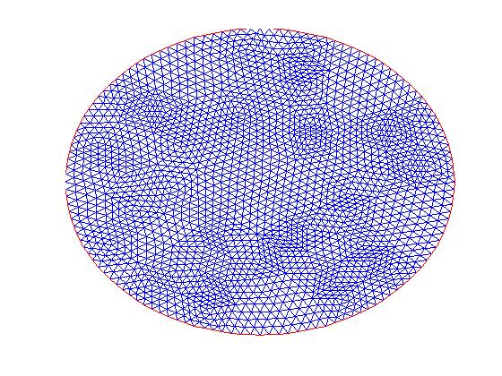
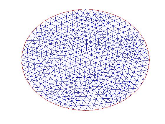
A                                                                                                                      B

Figure 1: A: Mesh containing 2097 triangles used for simulating measurements. B: Mesh containing 541 triangles used for the parameter reconstruction.

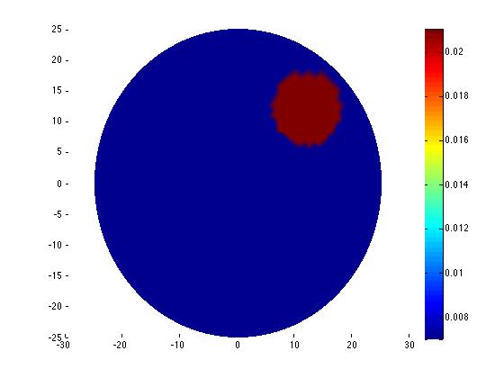
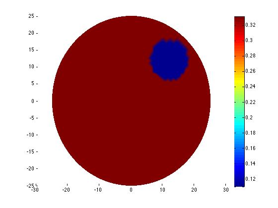
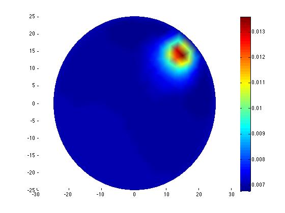
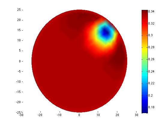
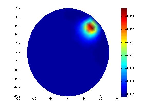
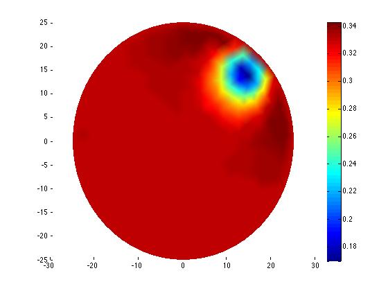
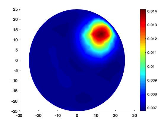
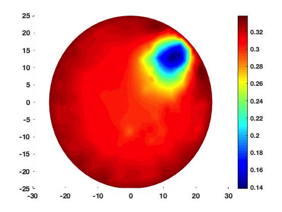
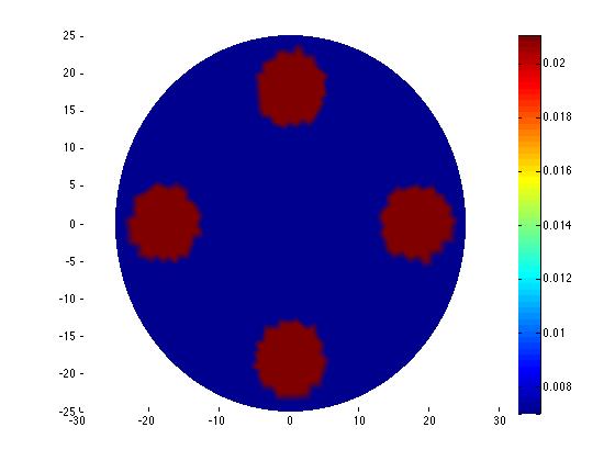
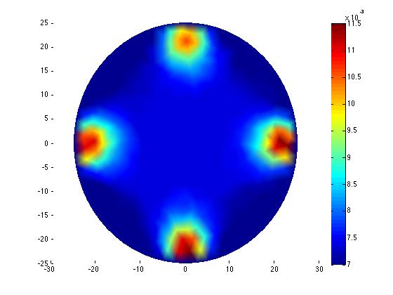
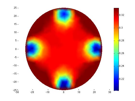
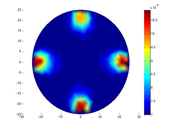
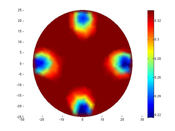
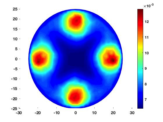
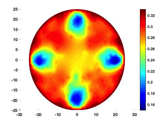
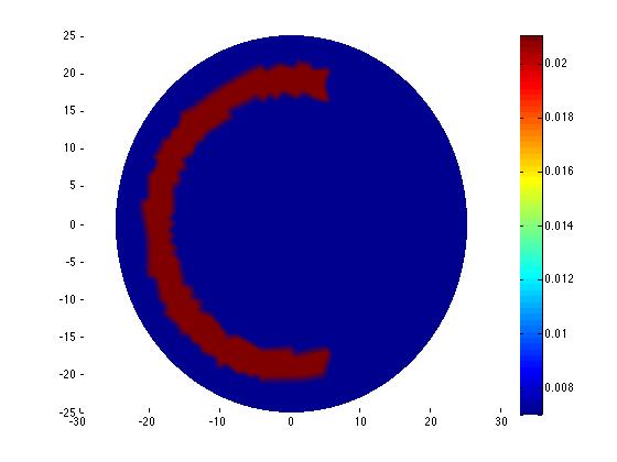
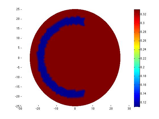
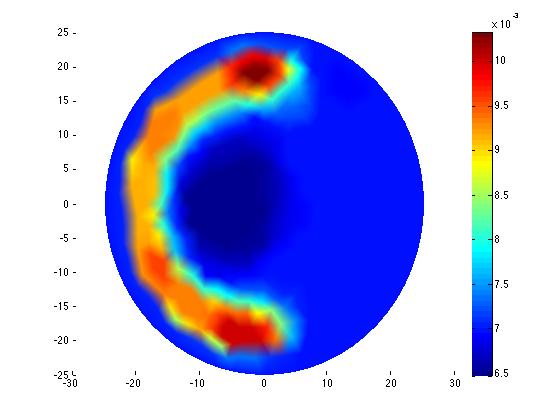
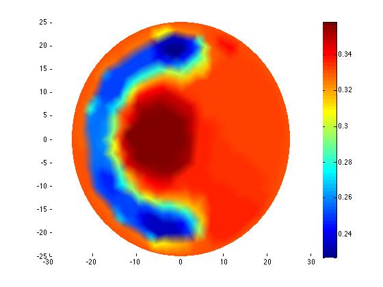
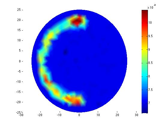
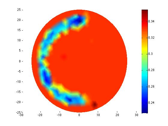
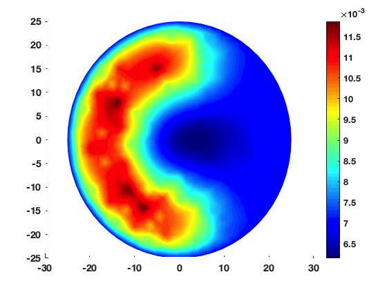
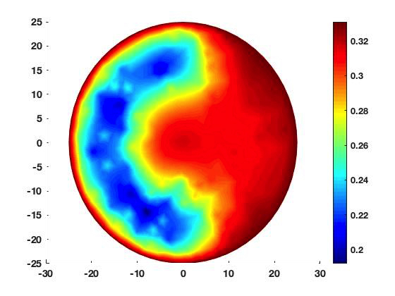
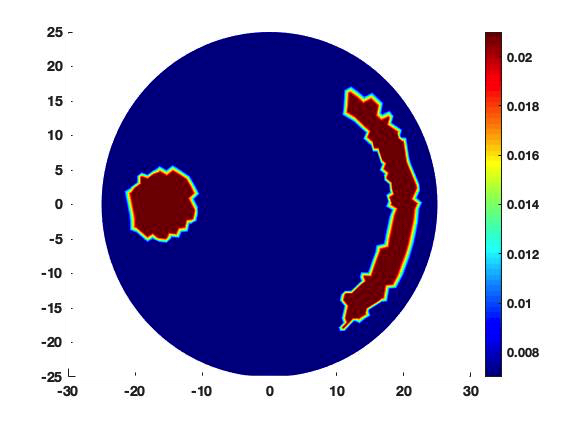
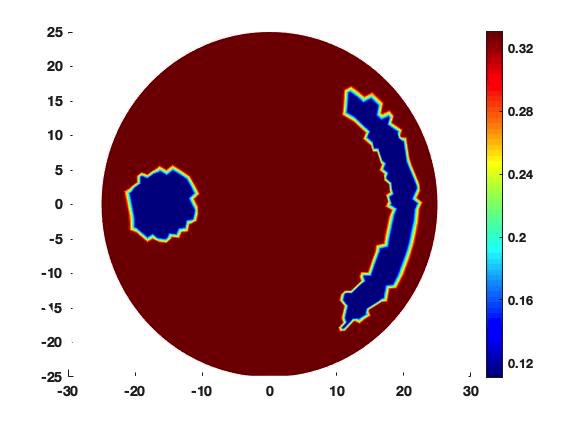
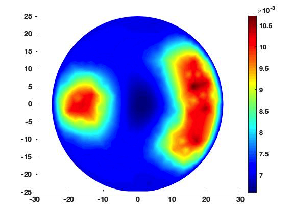
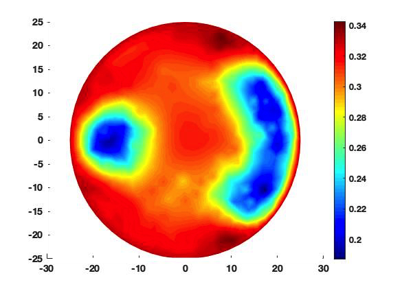
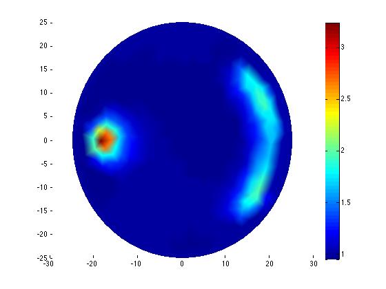
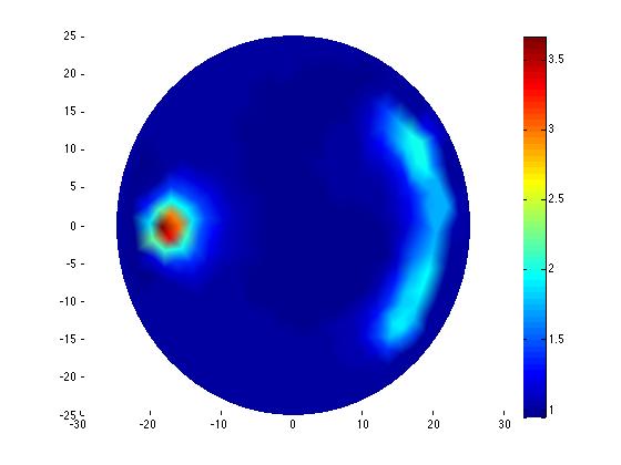
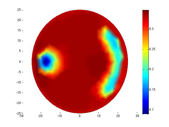
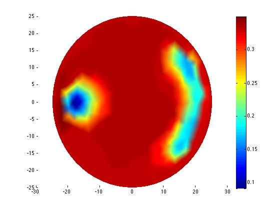
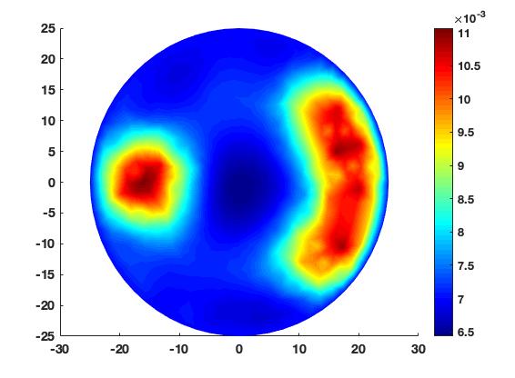
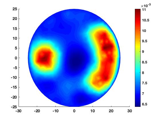
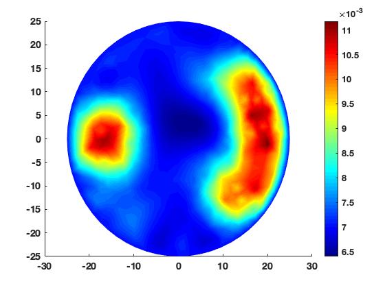
In figures 2-5, image A and B represent the true parameters $\mu$ and $D$ in mesh 1.A, images C-D and E-F are the corresponding reconstructions using the TV reconstruction (Section 6.2.2) and a mixture of the TV and the $\ell_{1}$ regularization (Equation 27) respectively from photon density measurements with $1\%$ additive relative Gaussian noise. It can be seen that both, the reconstructions with the TV, and the mixed TV and $\ell_{1}$, regularizations obtain relatively good reconstructions from the true parameters. However, in the presence of multiple inclusions (Figure 3) or more complex inclusions (Figure 4 and 5) the mixed regularizations seems to outperform the TV regularization. Note that in figures G-H, which represent reconstructions with the IRGN method, it can be seen that it performs similarly to the statistical methods in simple cases with one inclusion, but worse in setting with more complex inclusions.

A                                                                                                                                    B
C                                                                                                                                    D
E                                                                                                                                    F
G                                                                                                                                    H

Figure 2: A & B: The true parameters $\mu$ and $D$ in the simulation mesh (Figure 1.A). Reconstructions of the parameters $\mu$ and $D$ from measurements with $1\%$ additive Gaussian noise, C & D: using the TV regularization (Section 6.2.2). E & F: using a mixture of the TV and $\ell_{1}$ regularization (Equation 27). G & H: using IRGN Method.

A                                                                                                                                    B
C                                                                                                                                    D
E                                                                                                                                    F
G                                                                                                                                    H

Figure 3: A & B: The true parameters $\mu$ and $D$ in the simulation mesh (Figure 1.A). Reconstructions of the parameters $\mu$ and $D$ from measurements with $1\%$ additive Gaussian noise, C & D: using the TV regularization (Section 6.2.2). E & F: using a mixture of the TV and $\ell_{1}$ regularization (Equation 27). G & H: using IRGN Method.

A                                                                                                                                    B
C                                                                                                                                    D
E                                                                                                                                    F
G                                                                                                                                    H

Figure 4: A & B: The true parameters $\mu$ and $D$ in the simulation mesh (Figure 1.A). Reconstructions of the parameters $\mu$ and $D$ from measurements with $1\%$ additive Gaussian noise, C & D: using the TV regularization (Section 6.2.2). E & F: using a mixture of the TV and $\ell_{1}$ regularization (Equation 27). G & H: using IRGN Method.

A                                                                                                                                    B
C                                                                                                                                    D
E                                                                                                                                    F
G                                                                                                                                    H

Figure 5: A & B: The true parameters $\mu$ and $D$ in the simulation mesh (Figure 1.A). Reconstructions of the parameters $\mu$ and $D$ from measurements with $1\%$ additive Gaussian noise, C & D: using the TV regularization (Section 6.2.2). E & F: using a mixture of the TV and $\ell_{1}$ regularization (Equation 27). G & H: using IRGN Method.

Clearly, the reconstructions are strongly dependent on the choice of the regularization parameters. There is a vast literature for choosing optimal regularization parameters for linear problems. However, there are, to our knowledge, no good methods for nonlinear problems like DOT. Hence, we chose the parameters add hock. That is we used a computer cluster to run the algorithm with large set of regularization parameters choices, then we evaluated the reconstructions and picked the visually best parameters for the TV and the mixed regularizations. Note that once this parameter was found it was kept fixed for all reconstructions in figures 2-5.

Example	Example 1	Example 2	Example 3	Example 4
$\xi$	0.0018	0.0016	0.0016	0.0019
Residual, $E_{N}$	0.0124	0.010115	0.01335	0.01302
Residual, $E_{S}$	0.0129	0.0153	0.0139	0.0139

Table 1: Numerical results for noiselevel $\xi$ and residual error (i) $E_{N}$ using IRGN and (ii) $E_{S}$ using Statistical inversion for 1$\%$ noise

A                                                                                                  B                                                                                 C

D                                                                                                  E                                                                                 F

Figure 6: Reconstruction of $\mu$ and $D$ using statistical inversion method with, A, D: 5$\%$ noise, B, E: with 10$\%$ noise, C, F: with 20$\%$ relative additive Gaussian noise, respectively.

A                                                                                                  B                                                                                 C

D                                                                                                  E                                                                                 F

Figure 7: Reconstruction of $\mu$ and $D$ using IRGN method with, A, D: 5$\%$ noise, B, E: with 10$\%$ noise, C, F: with 20$\%$ relative additive Gaussian noise, respectively.

Relative	$L_{1}$ error	$L_{1}$ error	$L_{1}$ error	$L_{2}$ error	$L_{2}$ error	$L_{2}$ error
noise level	(TV)	(GR)	(IRGN)	(TV)	(GR)	(IRGN)
1%	0.1447	0.1337	0.1234	0.3245	0.3398	0.3230
5%	0.1439	0.1347	0.1206	0.3192	0.3423	0.3212
10%	0.1462	0.1355	0.1258	0.3272	0.3390	0.3257
15%	0.1442	0.1328	0.1315	0.3232	0.3368	0.3287
20%	0.1404	0.1358	0.1144	0.3129	0.3441	0.3268

Table 2: Relative Numerical Errors of $\mu$

Relative	$L_{1}$ error	$L_{1}$ error	$L_{1}$ error	$L_{2}$ error	$L_{2}$ error	$L_{2}$ error
noise level	(TV)	(GR)	(IRGN)	(TV)	(GR)	(IRGN)
1%	0.0625	0.0470	0.1002	0.1189	0.1227	0.1259
5%	0.0625	0.0455	0.0930	0.1161	0.1198	0.1192
10%	0.0638	0.0462	0.1159	0.1199	0.1216	0.1423
15%	0.0632	0.0449	0.1363	0.1204	0.1203	0.1653
20%	0.0598	0.0474	0.0923	0.1158	0.1242	0.1171

Table 3: Relative Numerical Errors of $D$

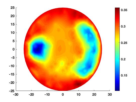
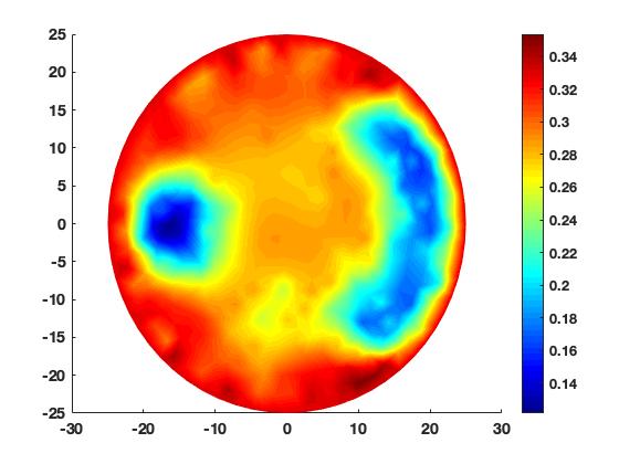
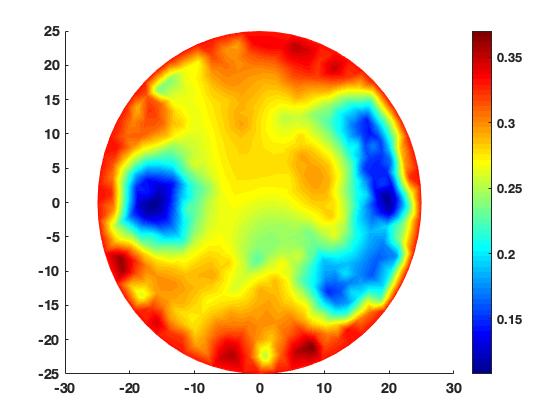
In Table 2 and 3 the relative error of reconstructions of $\mu$ and $D$ with different relative noise levels where computed. Note that the relative error of $\mu$ is defined as $\frac{||\mu_{t}-\mu_{r}||_{L_{p}}}{||\mu_{t}||_{L_{p}}}$, were $\mu_{t}$ represents the true parameter to be estimated and $\mu_{r}$ the reconstruction of $\mu_{t}$. The relative error of $D$ is defined analogous. In table 2 and 3 the relative $L_{1}$ and $L_{2}$ errors from the reconstructions using the Total Variation regularization (TV) defined in section 6.2.2, the General Regularization (GR) defined in (27) as well as with the IRGN method have been computed. As expected the reconstructions with using the Total Variation have mostly a smaller $L_{2}$ relative errors while reconstructions using the General Regularization have mostly a smaller $L_{1}$ relative errors. Furthermore, it can be seen that the presented method obtained relative good reconstructions up to a relative noise level from about $20\%$ (see figure 6). Note that the IRGN method generally seems to under-perform when comparing its relative error with the statistical methods. Moreover, the statistical inversion method and the IRGN method become unstable for higher noise level.

8 Conclusion

We presented a statistical formulation for the DOT inverse problem and compared it with the classical IRGN method. We found that from the visual point of view the statistical method outperforms the IRGN method up to high levels of relative noise. However, due to using the MCMC method the statistical solution is computational more intensive than the IRGN method.

The main contributions of this paper can be summarized in:

• To the best of our knowledge this is the first paper solving the Statistical Inverse problem for DOT.

• We introduce a mixture of the $TV$ and the $\ell_{p}$ regularization for the statistical DOT paper.

• We present many numerical experiments to evaluate the performance of the statistical inverse problem and compare it with the IRGN method as baseline.

References

- [1] Sanwar Ahmad, Thilo Strauss, Shyla Kupis, and Taufiquar Khan. Comparison of statistical inversion with iteratively regularized gauss newton method for image reconstruction in electrical impedance tomography. Applied Mathematics and Computation, 358:436–448, 2019.
- [2] S. R. Arridge and J. C. Schotland. Optical tomography: forward and inverse problems. Inverse Problems, 25(12):123010 (59pp), 2009.
- [3] Simon R. Arridge. Optical tomography in medical imaging. Inverse Problems, 15(2):R41–R93, 1999.
- [4] S.R. Arridge. Optical tomography in medical imaging: Topical review. Inverse Problems, 15:R41–R93, 1999.
- [5] S.R. Arridge and J.C. Hebden. Optical imaging in medicine: 2. modelling and reconstruction. Phys. Med. Biol., 42:841–853, 1997.
- [6] Anatoly Bakushinsky and Alexandra Smirnova. On application of generalized discrepancy principle to iterative methods for nonlinear ill-posed problems. Numerical Functional Analysis and Optimization, 26(1):35–48, 2005.
- [7] D.A. Boas, D.H. Brooks, E.L. Miller, C.A. DiMarzio, M. Kilmer, R.J. Gaudette, and Q. Zhang. Imaging the body with diffuse optical tomography. Signal Processing Magazine, IEEE, 18(6):57–75, 2001.
- [8] Liliana Borcea. Electrical impedance tomography. Inverse problems, 18(6):R99–R136, 2002.
- [9] S. Boyd and L. Vandenberghe. Convex Optimization. Cambridge University Press, London, 2004.
- [10] Stephen P Brooks and Andrew Gelman. General methods for monitoring convergence of iterative simulations. Journal of computational and graphical statistics, 7(4):434–455, 1998.
- [11] Florian Bürgel, Kamil S Kazimierski, and Armin Lechleiter. A sparsity regularization and total variation based computational framework for the inverse medium problem in scattering. Journal of Computational Physics, 339:1–30, 2017.
- [12] B. Chance and R. R. Alfano, editors. Photon Migration and Imaging in Random Media and Tissues, volume 1888 of (SPIE) Conference Series, September 1993.
- [13] B. Chance and R. R. Alfano, editors. Optical Tomography, Photon Migration, and Spectroscopy of Tissue and Model Media: Theory, Human Studies, and Instrumentation, volume 2389 of SPIE Conference Series, May 1995.
- [14] S. Chandrasekhar. Radiative Transfer. Dover, New York, 1960.
- [15] Siddhartha Chib and Edward Greenberg. Understanding the metropolis-hastings algorithm. The American Statistician, 49(4):327–335, 1995.
- [16] Eric T Chung, Tony F Chan, and Xue-Cheng Tai. Electrical impedance tomography using level set representation and total variational regularization. Journal of Computational Physics, 205(1):357–372, 2005.
- [17] D. T. Delpy and M. Cope. Quantification in tissue near-infrared spectroscopy. Phil. Trans. R. Soc. Lond. Ser. B, 352:649–659, June 1997.
- [18] T. Dierkes, O. Dorn, F. Natterer, V. Palamodov, and H. Sielschott. Fréchet derivatives for some bilinear inverse problems. SIAM Journal of Applied Mathematics, 62(6):2092–2113, 2002.
- [19] O. Dorn, E.L. Miller, and C.M. Rappaport. A shape reconstruction method for electromagnetic tomography using adjoint fields and level sets. Inverse Problems, 16:1119–1156, 2000.
- [20] Oliver Dorn. A transport-backtransport method for optical tomography. Inverse Problems, 14(5):1107, 1998.
- [21] Oliver Dorn. Shape reconstruction in scattering media with voids using a transport model and level sets. Canad. Appl. Math. Quart., 10(2):239–275, 2002.
- [22] Salaheddine El Adlouni, Anne-Catherine Favre, and Bernard Bobée. Comparison of methodologies to assess the convergence of markov chain monte carlo methods. Computational Statistics & Data Analysis, 50(10):2685–2701, 2006.
- [23] Alan E Gelfand and Sujit K Sahu. On markov chain monte carlo acceleration. Journal of Computational and Graphical Statistics, 3(3):261–276, 1994.
- [24] A Gelman, G Roberts, and W Gilks. Efficient metropolis jumping hules. Bayesian statistics, 5:599–608, 1996.
- [25] Andrew Gelman and Donald B Rubin. Inference from iterative simulation using multiple sequences. Statistical science, pages 457–472, 1992.
- [26] Edward I George and Robert E McCulloch. Variable selection via gibbs sampling. Journal of the American Statistical Association, 88(423):881–889, 1993.
- [27] A. P. Gibson, J. C. Hebden, and S. R. Arridge. Recent advances in diffuse optical imaging. Physics in Medicine and Biology, 50(4):R1–R43, 2005.
- [28] Walter R Gilks, Gareth O Roberts, and Sujit K Sahu. Adaptive markov chain monte carlo through regeneration. Journal of the American statistical association, 93(443):1045–1054, 1998.
- [29] Heikki Haario, Eero Saksman, and Johanna Tamminen. An adaptive metropolis algorithm. Bernoulli, pages 223–242, 2001.
- [30] W Keith Hastings. Monte carlo sampling methods using markov chains and their applications. Biometrika, 57(1):97–109, 1970.
- [31] J. C. Hebden, S. R. Arridge, and D. T. Delpy. Optical imaging in medicine: I. experimental techniques. Phys. Med. Biol., 42(5):825–840, 1997.
- [32] A.H. Hielscher, R.E. Alcouffe, and R.L. Barbour. Comparison of finite-difference transport and diffusion calculations for photon migration in homogeneous and heterogeneous tissues. Phys. Med. Biol., 43(5):1285–1302, 1998.
- [33] Bernd Hofmann, Barbara Kaltenbacher, Christiane Poeschl, and Otmar Scherzer. A convergence rates result for tikhonov regularization in banach spaces with non-smooth operators. Inverse Problems, 23(3):987, 2007.
- [34] A. Ishimaru. Single Scattering and Transport Theory: Wave Propogation and Scattering in Random Media I. Academic Press, New York, 1978.
- [35] Kazufumi Ito and Bangti Jin. A new approach to nonlinear constrained tikhonov regularization. Inverse Problems, 27(10):105005, 2011.
- [36] Kazufumi Ito, Bangti Jin, and Tomoya Takeuchi. A regularization parameter for nonsmooth tikhonov regularization. SIAM Journal on Scientific Computing, 33(3):1415–1438, 2011.
- [37] Kazufumi Ito, Bangti Jin, and Jun Zou. A new choice rule for regularization parameters in tikhonov regularization. Applicable Analysis, 90(10):1521–1544, 2011.
- [38] H. Jiang, V. Iftimia, Y. Xu, J. Eggert, L. Fajardo, and K. Klove. Near-infrared optical imaging of the breast with model-based reconstruction. Acad Radiol, 9:186–194, 2002.
- [39] Bangti Jin, Jun Zou, et al. Iterative parameter choice by discrepancy principle. IMA Journal of Numerical Analysis, page drr051, 2012.
- [40] Jari P Kaipio, Ville Kolehmainen, Erkki Somersalo, and Marko Vauhkonen. Statistical inversion and monte carlo sampling methods in electrical impedance tomography. Inverse problems, 16(5):1487, 2000.
- [41] Barbara Kaltenbacher and Bernd Hofmann. Convergence rates for the iteratively regularized gauss–newton method in banach spaces. Inverse Problems, 26(3):035007, 2010.
- [42] Barbara Kaltenbacher, Alana Kirchner, and Boris Vexler. Adaptive discretizations for the choice of a tikhonov regularization parameter in nonlinear inverse problems. Inverse Problems, 27(12):125008, 2011.
- [43] C.T. Kelley. Iterative Methods for Optimization. SIAM, Philadelphia, 1999.
- [44] T. Khan and A. Smirnova. 1d inverse problem in diffusion based optical tomography using iteratively regularized gauss-newton algorithm. Applied Mathematics and Computation, 161(1), 2005.
- [45] J. Koza. Genetic programmaing: on the programming of computers by means of natural selection. MIT Press, Boston, MA, 1992.
- [46] Armin Lechleiter, Kamil S Kazimierski, and Mirza Karamehmedović. Tikhonov regularization in lp applied to inverse medium scattering. Inverse Problems, 29(7):075003, 2013.
- [47] Nicholas Metropolis, Arianna W Rosenbluth, Marshall N Rosenbluth, Augusta H Teller, and Edward Teller. Equation of state calculations by fast computing machines. The journal of chemical physics, 21(6):1087–1092, 1953.
- [48] F. Natterer and F. Wübbeling. Mathematical Methods in Image Reconstruction. SIAM Monographs on Mathematical Modeling and Computation. Society for Industrial and Applied Mathematics (SIAM), Philadelphia, PA, 2001.
- [49] F. Natterer and F. Wübbeling. Mathematical Methods in Image Reconstruction. SIAM Monographs on Mathematical Modeling and Computation, 2001.
- [50] Frank Natterer, Helmut Sielschott, Oliver Dorn, Thomas Dierkes, and Victor Palamodov. Fréchet derivatives for some bilinear inverse problems. SIAM journal on applied mathematics, 62(6):2092–2113, 2002.
- [51] Jorge Nocedal and Stephen J Wright. Numerical Optimization Springer Series in Operations Research. Springer-Verlag New York Incorporated, 1999.
- [52] Y. Pei, H.L. Graber, and R.L. Barbour. Normalized-constraint algorithm for minimizing inter-parameter crosstalk in dc optical tomography. Optics Express, 9(2):97–109, 2001.
- [53] Adrian E Raftery and Steven M Lewis. Implementing mcmc. In Markov chain Monte Carlo in practice, pages 115–130. Springer, 1996.
- [54] Elena Resmerita. Regularization of ill-posed problems in banach spaces: convergence rates. Inverse Problems, 21(4):1303, 2005.
- [55] F. Santosa and M. Vogelius. A backprojection algorithm for electrical impedence imaging. SIAM J. Appl. Math., 50:216–243, 1990.
- [56] Thomas Schuster, Barbara Kaltenbacher, Bernd Hofmann, and Kamil S Kazimierski. Regularization methods in Banach spaces, volume 10. Walter de Gruyter, 2012.
- [57] A. Smirnova, R. Renaut, and T. Khan. Convergence and application of a modified iteratively regularized gauss-newton algorithm. Inverse Problems, 23(4):1547–1563, 2007.
- [58] Thilo Strauss. Statistical Inverse Problems in Electrical Impedance and Diffuse Optical Tomography. PhD thesis, CLEMSON UNIVERSITY, 2015.
- [59] Thilo Strauss, Xiaolin Fan, Shuyu Sun, and Taufiquar Khan. Statistical inversion of absolute permeability in single-phase darcy flow. Procedia Computer Science, 51:1188–1197, 2015.
- [60] Thilo Strauss and Taufiquar Khan. Statistical inversion in electrical impedance tomography using mixed total variation and non-convex ?p regularization prior. Journal of Inverse and Ill-posed Problems.
- [61] Thilo Strauss, Ruan Tao, Amir Poursaee, and Taufiquar Khan. Nondestructive testing of concrete using electrical impedance tomography with real data. Journal of Computational and Applied Mathematics, 2016.
- [62] John Sylvester and Gunther Uhlmann. A global uniqueness theorem for an inverse boundary value problem. Annals of mathematics, pages 153–169, 1987.
- [63] J. Tropp. Greed is good: Algorithmic results for sparse approximations. Technical Report, The University of Texas at Austin, 2003.
- [64] S. Walker, S. Fantini, and E. Gratton. Image reconstruction by backprojection from frequency-domain optical measurements in highly scattering media. Applied Optics, 36(1):170–179, 1997.