Communication-Efficient Distributed SVD via Local Power Iterations

Abstract

We study distributed computing of the truncated singular value decomposition problem. We develop an algorithm that we call LocalPower for improving communication efficiency. Specifically, we uniformly partition the dataset among $m$ nodes and alternate between multiple (precisely $p$) local power iterations and one global aggregation. In the aggregation, we propose to weight each local eigenvector matrix with orthogonal Procrustes transformation (OPT). As a practical surrogate of OPT, sign-fixing, which uses a diagonal matrix with $\pm 1$ entries as weights, has better computation complexity and stability in experiments. We theoretically show that under certain assumptions LocalPower lowers the required number of communications by a factor of $p$ to reach a constant accuracy. We also show that the strategy of periodically decaying $p$ helps obtain high-precision solutions. We conduct experiments to demonstrate the effectiveness of LocalPower.

1 Introduction

In this paper we consider the truncated singular value decomposition (SVD) which has broad applications in machine learning, such as dimension reduction [51], matrix completion [8], and information retrieval [14]. Let ${\bf a}_{1},\cdots,{\bf a}_{n}\in{\mathbb{R}}^{d}$ be sampled i.i.d. from some fixed but unknown distribution. The goal is to compute the $k$ ($k<\min\{d,n\}$) singular vectors of ${\bf A}\triangleq[{\bf a}_{1},\ldots,{\bf a}_{n}]^{\top}\in{\mathbb{R}}^{n\times d}$. Let ${\bf V}_{k}\in{\mathbb{R}}^{d\times k}$ contain the top $k$ singular vectors. The power iteration and its variants such as Krylov subspace iterations are common approaches to the truncated SVD. They have ${\mathcal{O}}(nd)$ space complexity and ${\mathcal{O}}(ndk)$ per-iteration time complexity. They take $\tilde{{\mathcal{O}}}(\log\frac{d}{\epsilon})$ iterations to converge to $\epsilon$ precision, where $\tilde{{\mathcal{O}}}$ hides the spectral gap and constants [22, 37].

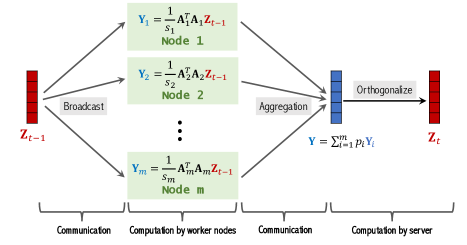
When either $n$ or $d$ is big, the data matrix ${\bf A}\in{\mathbb{R}}^{n\times d}$ may not fit in the memory, making standard single-machine algorithms infeasible. A distributed power iteration is feasible and practical for large-scale truncated SVDs. In particular, we partition the rows of ${\bf A}$ among $m$ worker nodes (see Figure 1(a)) and let the nodes perform power iterations in parallel (see Figure 1(b)). In every iteration, every node performs ${\mathcal{O}}(\frac{ndk}{m})$ FLOPs (suppose the load is balanced), while the server performs only ${\mathcal{O}}(dk^{2})$ FLOPs.

When solving large-scale matrix computation problems, communication costs are not negligible; in fact, communication costs can outweigh computation costs. The large-scale SVD experiments in [21, 50] show that the runtime caused by communication and straggler’s effect can exceed the computation time. Due to the communication costs and other overheads, parallel computing can even demonstrate anti-scaling; that is, when $m$ is big, the overall wall-clock runtime increases with $m$. Reducing the frequency of communications will reduce the communication and synchronization costs and thereby improving the scalability.

(a) Partition.

(b) Standard parallel power iteration (DPI).

(c) Commonly used symbols

Figure 1: (a) The $n\times d$ data matrix ${\bf A}$ is partitioned among $m$ worker nodes. (b) In every iteration of the distributed power iteration, there are two rounds of communications. Most of the computations are performed by the worker nodes. (c) Commonly used symbols.

1.1 Our Contributions

Inspired by the FedAvg algorithm [32], we propose an algorithm called LocalPower to improve communication-efficiency. LocalPower is based on the distributed power iteration (DPI) described in Figure 1. The difference is that LocalPower makes every node locally perform orthogonal iterations using its own data for $p$ iterations. In the case for $p=1$, LocalPower degenerates to DPI. When $p\geq 2$, local updates are employed to reduce communication frequency.

In practice, a naive implementation of the proposed LocalPower does not work very well. We propose three effective techniques for improving LocalPower:

• We propose to decay the communication interval, $p$, over time. In this way, the loss drops fast in the beginning and converge to the optimal solution in the end. Without the decay strategy, LocalPower is not guaranteed to converge to the optimum.

• Orthogonal Procrustes transformation (OPT) post-processes the output matrices of the $m$ nodes after each iteration so that the $m$ matrices are close to each other. OPT makes LocalPower stable at the cost of more computation.

• To reduce the computation of OPT, we replace its orthogonal space to the set of all diagonal matrices with $\pm 1$ entries. In this way, OPT becomes the sign-fixing technique which is stable (slightly worse than OPT) and efficient. Sign fixing was originally proposed by Garber et al. [19] for the special case of $k=1$, while we generalize sign-fixing to $k>1$.

In summary, this work’s contributions include the new algorithm, LocalPower, its convergence analysis, and the effective techniques for improving LocalPower.

The remainder of this paper is organized as follows. In Section 2, we define notation and give preliminary backgrounds on the orthogonal Procrustes problem and the distributed power iteration. In Section 3, we propose LocalPower and its variants and then provide theoretical analysis in Section 4. In Section 5, we conduct experiments to illustrate the effectiveness of LocalPower and to validate our theoretical results. In Section 6, we give further discussions on some aspects of LocalPower. All proof details can be found at Appendix A. In Appendix D, we discuss related work on SVD and parallel algorithms.

2 Preliminary

Notation.

For any ${\bf A}\in{\mathbb{R}}^{n\times d}$, we use $\|{\bf A}\|_{2}$ and $\|{\bf A}\|_{F}$ to denote its spectral norm and Frobenius norm. Let ${\bf A}^{\dagger}\in{\mathbb{R}}^{d\times n}$ denote the Moore-Penrose pseudo-inverse of ${\bf A}$. For any positive integer $T$, let $[T]=\{1,2,\cdots,T\}$. ${\mathcal{O}}_{d\times k}$ is the set of all $d\times k$ column orthonormal matrices ($1\leq k\leq d$). ${\mathcal{O}}_{k}$, short for ${\mathcal{O}}_{k\times k}$, denotes the set of $k\times k$ orthogonal matrices. ${\mathcal{R}}({\bf U})$ denotes the subspace spanned by the columns of ${\bf U}$. The commonly used notation is summarized in Figure 1(c).

Power iteration.

The top $k$ right singular vectors of ${\bf A}$ can be obtained by the subspace iteration that repeats

$${\bf Y}\>\longleftarrow\>{\bf M}{\bf Z}\quad\textrm{ and }\quad{\bf Z}\>\longleftarrow\>\mathsf{orth}\big{(}{\bf Y}\big{)},$$ (1)

where ${\bf M}=\frac{1}{n}{\bf A}^{\top}{\bf A}$. In every power iteration, computing ${\bf Y}$ has ${\mathcal{O}}(ndk)$ time complexity, and orthogonalizing ${\bf Y}$ has ${\mathcal{O}}(dk^{2})$ time complexity. It is well known that the tangent of principle angles between ${\mathcal{R}}({\bf Z})$ and ${\mathcal{R}}({\bf U}_{k})$ converges to zero geometrically [2, 37] and thus so their projection distance.

Distributed power iteration (DPI)

is a direct distributed variant of power iteration. Consider data parallelism and partition the data (rows of ${\bf A}$) among $m$ worker nodes. See Figure 1(a) for the illustration. We partition ${\bf A}$ as ${\bf A}^{\top}=[{\bf A}_{1}^{\top},\cdots,{\bf A}_{m}^{\top}]$ where ${\bf A}_{i}\in{\mathbb{R}}^{s_{i}\times d}$ contains $s_{i}$ rows of ${\bf A}$. Using $m$ worker nodes and data parallelism, one power iteration works in four steps. First, the server broadcasts ${\bf Z}$ to the workers, which has ${\mathcal{O}}(dk)$ or ${\mathcal{O}}(dkm)$ communication complexity (depending on the network structure). Second, every worker (say, the $i$-th) locally computes

$${\bf Y}_{i}={\bf M}_{i}{\bf Z}\in{\mathbb{R}}^{d\times k}\quad\textrm{ with }\quad{\bf M}_{i}=\frac{1}{s_{i}}{\bf A}_{i}^{\top}{\bf A}_{i},$$ (2)

which has ${\mathcal{O}}(d^{2}k)$ or ${\mathcal{O}}(s_{i}dk)$ time complexity. Third, the server aggregates ${\bf Y}_{i}$, for all $i\in[m]$, to obtain ${\bf Y}=\sum_{i=1}^{m}p_{i}{\bf Y}_{i}$; this step is equivalent to ${\bf Y}={\bf M}{\bf Z}$, where ${\bf M}=\sum_{i=1}^{m}p_{i}{\bf M}_{i}$ with $p_{i}=\frac{s_{i}}{n}$. It has ${\mathcal{O}}(dk)$ or ${\mathcal{O}}(dkm)$ communication complexity. Last, the server locally orthogonalizes ${\bf Y}$ to obtain ${\bf Z}=\mathsf{orth}({\bf Y})$, which has merely ${\mathcal{O}}(dk^{2})$ time complexity. The algorithm is described in Figure 1(b). The following lemma is a well-known result [2, 37].

Lemma 1.

To obtain a column-orthonormal matrix ${\bf Z}$ such that the subspace distance $\text{dist}({\bf Z},{\bf U}_{k})\leq\epsilon$ (see Definition 1 for detail), with high probability, the communication needed by DPI is

$$\Omega\left(\frac{\sigma_{k}}{\sigma_{k}-\sigma_{k+1}}\log\left(\frac{d}{\epsilon}\right)\right).$$ (3)

Here, $\sigma_{j}$ is the $j$-th largest singular value of the matrix ${\bf M}$.

3 Algorithms

Algorithm 1 LocalPower

1:  Input: distributed dataset $\{{\bf A}_{i}\}_{i=1}^{m}$, target rank $k$, iteration rank $r\geq k$, number of iterations $T$.

2:  Initialization: generate a standard Gaussian matrix, ${\bf Y}_{0}$;

3:  for $t=0$ to $T$ do

4:     Broadcast: If $t\in{\mathcal{I}}_{T}$, the server sends ${\bf Y}_{t}$ to workers; let ${\bf Y}_{t}^{(i)}\leftarrow{\bf Y}_{t}$;

5:     Local computation: For all $i\in[m]$, the $i$-th worker locally computes

$${\bf Z}_{t}^{(i)}=\mathsf{orth}({\bf Y}_{t}^{(i)})\quad\textrm{and}\quad{\bf Y}_{t+1}^{(i)}=\tfrac{1}{s_{i}}{\bf A}_{i}^{\top}{\bf A}_{i}{\bf Z}_{t}^{(i)};\vspace{-2mm}$$

6:     Aggregation: If $(t+1)\in{\mathcal{I}}_{T}$, the server computes ${\bf Y}_{t+1}=\sum_{i=1}^{m}p_{i}{\bf Y}_{t+1}^{(i)}$;

7:  end for

8:  Output: $\mathsf{orth}({\bf Y}_{t+1})$.

LocalPower

is a new algorithm that we propose for improving communication efficiency. It is described in Algorithm 1. Its basic idea is to trade more local power iterations for fewer communications via reducing the communication frequency. Between two communications, every worker node locally runs eqn. (2) for multiple times. We let the set ${\mathcal{I}}_{T}$ ($\subseteq[T]$) index the iterations that perform communications; for example,

$${\mathcal{I}}_{T}\;=\;\big{\{}0,p,2p,\cdots,T\big{\}}$$

means that the algorithm communicates once after $p$ lower power iterations. The cardinality $|{\mathcal{I}}_{T}|$ is the total number of communications.

Suppose LocalPower performs one communication every $p$ iterations. In $T$ iterations, each worker performs ${\mathcal{O}}(s_{i}dkT)$ FLOPs, the server performs ${\mathcal{O}}(dk^{2}T/p)$ FLOPs, and the overal communication complexity is ${\mathcal{O}}(dkT/p)$. The standard distributed power iteration is a special case of LocalPower with $p=1$, that is, ${\mathcal{I}}_{T}=\{0,1,2,\cdots,T\}$. One-shot SVD, aka divide-and-conquer SVD, [31, 19, 15], is a special case of LocalPower with $p=T$, that is, ${\mathcal{I}}_{T}=\{0,T\}$.

Decaying $p$.

In practice, it is helpful to use a big $p$ in the beginning but let $p=1$ in the end. For example, we can decrease $p$ by half every few communications. The rationale is that the error of LocalPower does not converge to zero if $p$ is big; see the theoretical analysis in the next section. Our empirical observation confirms the theories: if $p$ is set big, then the error drops very fast in the beginning, but it does not vanish with the iterations.

Orthogonal Procrustes Transformation.

In Algorithm 1, the $i$-th worker locally computes

$${\bf Y}_{t+1}^{(i)}\;=\;\tfrac{1}{s_{i}}{\bf A}_{i}^{\top}{\bf A}_{i}{\bf Z}_{t}^{(i)}.$$

When it comes to the time of communication (i.e., $t+1\in{\mathcal{I}}_{T}$), we replace the equation by the following steps. First, we choose the device which has the maximum number of samples as a base. Without loss of generality, we can assume the first device is selected (which indicates $1=\mathop{\rm argmin}_{i\in[m]}p_{i})$. Second, we compute

$${\bf O}_{t}^{(i)}\;=\;\mathop{\rm argmin}_{{\bf O}\in{\mathcal{O}}_{k}}\;\big{\|}{\bf Z}^{(i)}_{t}{\bf O}-{\bf Z}^{(1)}_{t}\big{\|}_{F}^{2}.$$ (4)

Eqn. (4) is a classic matrix approximation problem in linear algebra, named as the Procrustes problem [38, 9]. The solution to eqn. (4) is referred to as orthogonal Procrustes transformation (OPT) and has a closed form:

$${\bf O}_{t}^{(i)}\;=\;{\bf W}_{1}{\bf W}_{2}^{\top},$$

where ${\bf W}_{1}\mbox{\boldmath$\Sigma$\unboldmath}{\bf W}_{2}^{\top}$ is the SVD of $({\bf Z}^{(i)}_{t})^{\top}{\bf Z}^{(1)}_{t}$. Finally, we compute

$${\bf Y}_{t+1}^{(i)}\;=\;\tfrac{1}{s_{i}}{\bf A}_{i}^{\top}{\bf A}_{i}{\bf Z}_{t}^{(i)}{\bf O}_{t}^{(i)}.$$

Remak 1.

Intuitively, such ${\bf O}_{t}^{(i)}$ adjusts ${\bf Z}_{t}^{(i)}$ such that it aligns with ${\bf Z}_{t}^{(1)}$ better. In an ideal case, all ${\bf Z}_{t}^{(i)}$’s would be identical with ${\bf Z}_{t}^{(1)}$ and thus the aggregation step (line 6 in Algorithm 1) would be the same as that in DPI . From our theory, it is important to use OPT. It weakens the assumption on the smallness of a residual error which is incurred by local computation. From our experiments, it stabilizes vanilla LocalPower and achieves much smaller errors.

Remak 2.

To compute such ${\bf O}_{t}^{(i)}$, the $i$-th client should communicate ${\bf Z}_{t}^{(i)}$ to the server, which results in additional communication cost. However, the cost is the same in magnitude as that of sending ${\bf Y}_{t+1}^{(i)}$ in the aggregation step. Besides, the computation of ${\bf O}_{t}^{(i)}$ as well as the communication of ${\bf Y}_{t+1}^{(i)}$ only happens when $t+1\in{\mathcal{I}}_{T}$. These make the additional communication cost affordable.

Sign-Fixing.

While OPT makes LocalPower more stable in practice, OPT incurs more local computation. Specifically, it has time complexity ${\mathcal{O}}(dk^{2})$ via calling the SVD of $({\bf Z}^{(i)}_{t})^{\top}{\bf Z}^{(1)}_{t}$. To attain both efficiency and stability, we propose to replace the $k\times k$ matrix ${\bf O}^{(i)}$ in eqn. (4) by

$${\bf D}_{t}^{(i)}\;=\;\mathop{\rm argmin}_{{\bf D}\in{\mathcal{D}}_{k}}\;\big{\|}{\bf Z}^{(i)}_{t}{\bf D}-{\bf Z}^{(1)}_{t}\big{\|}_{F}^{2},$$ (5)

where ${\mathcal{D}}_{k}$ denotes all the $k\times k$ diagonal matrices with $\pm 1$ diagonal entries. ${\bf D}_{t}^{(i)}$ can be computed in ${\mathcal{O}}(kd)$ time by

$${\bf D}_{t}^{(i)}[j,j]\;=\;\mathrm{sgn}\Big{(}\,\Big{\langle}{\bf Z}^{(i)}_{t}[:,j]\,,\>{\bf Z}^{(1)}_{t}[:,j]\Big{\rangle}\,\Big{)},\quad\forall\;j\in[k].$$

We empirically observe that sign-fixing serves as a good practical surrogate of OPT; it maintains good stability and achieves comparably small errors.

Remak 3.

If we decay $p$, $p$ will drop to one after a few communications. When $p=1$, we stop using OPT (or sign-fixing); we simply set ${\bf O}_{t}^{(i)}$ (or ${\bf D}_{t}^{(i)}$) to the identity matrix.

Remak 4.

The technique of sign-fixing has been proposed in the setting of $k=1$ by Garber et al. [19]. In the $k=1$ setting, OPT and sign-fixing coincide with each other. In eqn. (5), we provide a simple way to extend it to high-dimensional $k>1$. We compute ${\bf D}_{t}^{(i)}$ that simultaneously adjusts the signs of columns of ${\bf Z}_{t}^{(i)}$ and ${\bf Z}_{t}^{(1)}$. There exists other way to handle the high-dimensional sign-fixing problem. For example, if first $k$ eigenvalues are well-separated from others, we can reduce the top-$k$ sign-fixing problem to the one-dimensional sign-fixing problem instanced $k$ times.

4 Convergence Analysis

In this section we analyze the convergence of LocalPower and show the benefit of OPT under an ideal setting. We use the projection distance of two subspaces as the metric for convergence evaluation.

Definition 1 (Projection Distance).

Let ${\bf U},{\widetilde{{\bf U}}}\in{\mathcal{O}}_{d\times k}$ be any matrices with orthonormal columns. The projection distance between them is

$$\operatorname{dist}({\bf U},{\widetilde{{\bf U}}})\;\triangleq\;\big{\|}{\bf U}{\bf U}^{\top}-{\widetilde{{\bf U}}}{\widetilde{{\bf U}}}^{\top}\big{\|}_{2}.$$

Projection distance is equivalent to $\operatorname{dist}({\bf U},{\widetilde{{\bf U}}})=\sin\theta_{k}({\bf U},{\widetilde{{\bf U}}})$ where $\theta_{k}({\bf U},{\widetilde{{\bf U}}})$ denotes the $k$-th largest principal angle between the subspaces spanned by ${\bf U}$ and ${\widetilde{{\bf U}}}$. Principal angles quantify how different two subspaces are. We can actually calculate

$$\theta_{1}\big{(}{\bf U},{\widetilde{{\bf U}}}\big{)},\;\;\theta_{2}\big{(}{\bf U},{\widetilde{{\bf U}}}\big{)},\;\;\cdots,\;\theta_{k}\big{(}{\bf U},{\widetilde{{\bf U}}}\big{)}$$

via the SVD of ${\bf U}^{\top}{\widetilde{{\bf U}}}$. The $l$-th largest singular value of ${\bf U}^{\top}{\widetilde{{\bf U}}}$ is equal to $\cos\theta_{l}({\bf U},{\widetilde{{\bf U}}})$ for all $l=1,\cdots,k$.

Definition 2 (Local Approximation).

Let ${\bf M}_{i}=\frac{1}{s_{i}}{\bf A}_{i}^{\top}{\bf A}_{i}$ be hosted by the $i$-th worker. Let ${\bf M}=\frac{1}{n}\sum_{i=1}^{m}{\bf A}_{i}^{\top}{\bf A}_{i}=\sum_{i=1}^{m}p_{i}{\bf M}_{i}$. Define

$$\eta\;\triangleq\;\max_{i\in[m]}\frac{\|{\bf M}_{i}-{\bf M}\|_{2}}{\|{\bf M}\|_{2}},$$

which measures how far the local matrices, ${\bf M}_{1},\cdots,{\bf M}_{m}$, are from ${\bf M}$. If $s_{i}=p_{i}n$ is sufficiently larger than $d$, then $\eta$ is sufficiently small.

Definition 3 (Residual Error).

If OPT is not used, define

$$\rho_{t}\;\triangleq\;\max_{i\in[m]}\big{\|}{\bf Z}_{t}^{(i)}-{\bf Z}_{t}^{(1)}\big{\|}_{2}.$$

If OPT is used, define

$$\rho_{t}\;\triangleq\;\max_{i\in[m]}\min_{{\bf O}\in{\mathcal{O}}_{k}}\big{\|}{\bf Z}_{t}^{(i)}{\bf O}-{\bf Z}_{t}^{(1)}\big{\|}_{2}.$$

The residual error $\rho_{t}$ measures how the local top-$k$ eigenspace estimator varies across the $m$ worker. Based on the definition, using OPT makes $\rho_{t}$ smaller than without using OPT. When $t\in{\mathcal{I}}_{T}$, ${\bf Z}_{t}^{(1)}=\cdots={\bf Z}_{t}^{(m)}$ and thus $\rho_{t}=0$. When $t\notin{\mathcal{I}}_{T}$, each local update would enlarge $\rho_{t}$. Hence, intuitively $\rho_{t}$ depends on $p$, i.e., the local iterations between two communications. However, later we will show that with OPT $\rho_{t}$ does not depend on $p$ (when $p$ is sufficiently large) while it depends on $p$ without OPT. A residual error is inevitable in previous literature of empirical risk minimization that uses local updates to improve communication efficiency [42, 48, 56, 29, 30]. In our case, it takes the form of $\rho_{t}$.

Assumption 1 (Uniformly small residual errors).

Let $r$ be the running column number, $\sigma_{j}$ be the $j$-th largest singular value of ${\bf M}$, and $\epsilon\in(0,0.5)$ be a constant. Assume $\eta\leq\frac{1}{3\kappa}$ where $\kappa=\|{\bf M}\|\|{\bf M}^{\dagger}\|$ is the condition number of ${\bf M}$. Assume for all $t\in[T]$,

$$\eta\cdot 1_{t\notin{\mathcal{I}}_{T}}+(1-p_{\max})(\rho_{t}+\rho_{t-1}1_{t\notin{\mathcal{I}}_{T}})\;=\;{\mathcal{O}}(\epsilon_{0}),$$ (6)

where $p_{\max}=\max_{i\in[m]}p_{i}$, $1_{t\notin{\mathcal{I}}_{T}}$ is the indication function of the event $\{t\notin{\mathcal{I}}_{T}\}$, and

$$\epsilon_{0}\;\triangleq\;\frac{\sigma_{k}-\sigma_{k+1}}{\sigma_{1}\kappa}\min\left\{\frac{\sqrt{r}-\sqrt{k-1}}{\tau\sqrt{d}},\epsilon\right\}$$

for some small constant $\tau>0$.

Theorem 1 (Convergence for LocalPower).

Let $\tau$ be a positive constant, and Assumption 1 hold. Then, after $|{\mathcal{I}}_{T}|$ rounds of communication where

$$T=\Omega\left(\frac{\sigma_{k}}{\sigma_{k}-\sigma_{k+1}}\log\left(\frac{\tau d}{\epsilon}\right)\right),$$

with probability at least $1-\tau^{-\Omega(r+1-k)}-e^{-\Omega(d)}$, we have

$$\operatorname{dist}({\bf Z}_{T},{\bf U}_{k})=\sin\theta_{k}({\bf Z}_{T},{\bf U}_{k})\leq\epsilon.$$

Theorem 1 shows LocalPower takes $T=\widetilde{\Theta}\left(\frac{\sigma_{k}}{\sigma_{k}-\sigma_{k+1}}\right)$ iterations to obtain an $\epsilon$-optimal solution, the same quantity required by DPI . However, LocalPower uses less communications. For example, with ${\mathcal{I}}_{T}=\{0,p,2p,\cdots,T\}$, LocalPower makes only $|{\mathcal{I}}_{T}|\>=\>\widetilde{\Theta}\left(\frac{1}{p}\frac{\sigma_{k}}{\sigma_{k}-\sigma_{k+1}}\right)$ communications, saving a factor of $p$ than DPI .

Theorem 1 depends on Assumption 1 which requires eqn. (6) holds for all $t\in[T]$. What’s more, the final error $\epsilon$ is positively related to $\eta$ and $\rho_{t}$ via eqn. (6). The first part of eqn. (6) (i.e., $\eta\cdot 1_{t\notin{\mathcal{I}}_{T}}$) is incurred by the variety of ${\bf M}_{i}$’s. So, if all devices have access to ${\bf M}$ (which implies ${\bf M}_{1}=\cdots={\bf M}_{m}$), then it would vanish. The second part eqn. (6) is brought by intermittent communication. Indeed, if communication happens at iteration $t$ (i.e., $t\in{\mathcal{I}}_{T}$), we have $\rho_{t}=0$ and $1_{t\notin{\mathcal{I}}_{T}}=0$, implying  eqn. (6) holds obviously. Without communication, $\rho_{t}$ is likely to grow continually, which is harmful to obtaining an accurate solution. Therefore, the assumption actually requires the communication interval $p$ is not too large. From another hand, when $p$ is fixed, the assumption instead imposes restriction on $\eta$ when $t\notin{\mathcal{I}}_{T}$, because we show in Theorem 2 that $\rho_{t}$ is bounded by a function of $\eta$. If OPT is used, then $\rho_{t}={\mathcal{O}}(\eta)$, without dependence on $p$. However, if OPT is not used, then $\rho_{t}={\mathcal{O}}(\sqrt{k}p\kappa^{p}\eta)$ has an exponential dependence on $p$.

Theorem 2 (Benefits of OPT).

Let $\tau(t)\in{\mathcal{I}}_{T}$ be the nearest communication time before $t$ and $p=t-\tau(t)$. Let $\mathrm{e}$ be the natural constant. Assume $\eta\leq\min(\frac{1}{3\kappa},\frac{1}{p})$.

• With OPT, $\rho_{t}$ is bounded by

  $$\min\left\{2\mathrm{e}^{2}\kappa^{p}p\eta,\frac{\eta\sigma_{1}}{\delta_{k}}+2\gamma_{k}^{p/4}C_{t}\right\}={\mathcal{O}}(\eta),$$

  where $\gamma_{k}\in(0,1)$, $\delta_{k}=\Theta(\sigma_{k}-\sigma_{k+1})$, and $\limsup_{t}C_{t}={\mathcal{O}}(\eta+\epsilon)$.

• Without OPT, $\rho_{t}$ is bounded by

  $$4\mathrm{e}\sqrt{k}p\kappa^{p}\eta={\mathcal{O}}(\sqrt{k}p\kappa^{p}\eta).$$

Why using OPT has such an exponential improvement on dependence on $p$ in theory? This is mainly because of the property of OPT. Let ${\bf O}^{*}=\mathop{\rm argmin}_{{\bf O}\in{\mathcal{O}}_{k}}\|{\bf U}-{\widetilde{{\bf U}}}{\bf O}\|_{F}$ for ${\bf U},{\widetilde{{\bf U}}}\in{\mathcal{O}}_{d\times k}$. Then, up to some universal constant, we have $\|{\bf U}-{\widetilde{{\bf U}}}{\bf O}^{*}\|_{2}\approxeq\operatorname{dist}({\bf U},{\widetilde{{\bf U}}}).$ See Lemma 3 in Appendix for a formal statement and detailed proof. It implies up to a tractable orthonormal transformation, the difference between the orthonormal bases of two subspaces is no larger than the projection distance between the subspaces. By the Davis-Kahan theorem (see Lemma 11), their projection distance is not larger than ${\mathcal{O}}(\eta)$ up to some problem-dependent constants. However, without OPT, we have to use perturbation theory to bound $\rho_{t}$, which inevitably results in exponential dependence on $p$.

5 Experiments

Settings.

We use 15 datasets available on the LIBSVM website. The $n$ data samples are randomly shuffled and then partitioned among $m$ nodes so that each node has $s=\frac{n}{m}$ samples. We set $m=\max(\lfloor\frac{n}{1000}\rfloor,3)$ so that each node has $s=1,000$ samples, unless $n$ is too small. The features are normalized so that all the values are between $-1$ and $1$. All the algorithms start from the same initialization ${\bf Y}_{0}$. We fix the target rank to $k=5$. Our focus is on communication efficiency, so we use communication rounds for evaluating the compared algorithms. Due to the space limit, we defer more experiment details and additional experiment results to Appendix E.

Compared algorithms.

We evaluate three variants of LocalPower : the vanilla version, with OPT, and with sign-fixing. We compare our algorithms with one-shot algorithms, UDA [15], WDA [6], and DR-SVD; the algorithms are described in Appendix E.2.

Final precision.

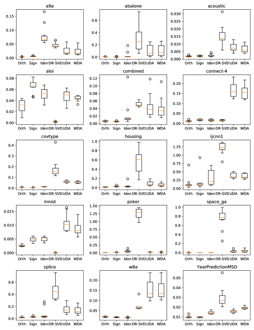
In this set of experiments, we study the precision when the algorithms converge. For three variants of LocalPower   we fix $p=4$ (without decaying $p$). We run each algorithm 10 times and report the mean and standard deviation (std) of the final errors. Due to limited space, Table 1 shows the results on 7 datasets. Table 6 and Figure 11 (in the appendix) present all the results on the 15 datasets. Out of the 15 datasets, LocalPower has the smallest error mean and std on 12 datasets. The results indicate that one-shot methods do not find high-precision solutions unless the local data size is sufficiently large.

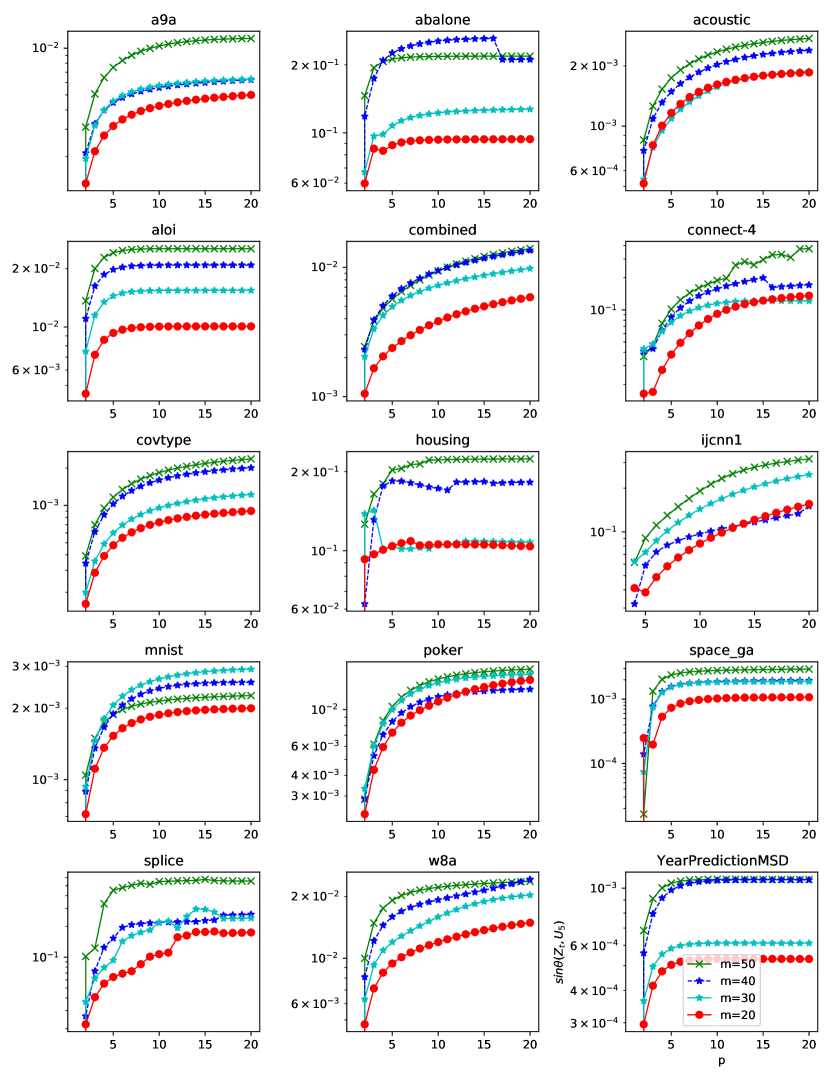
The final error depends on $p$. With $p>1$, the final error, $\lim_{t\rightarrow\infty}\sin\theta_{k}({\bf Z}_{t},{\bf U}_{k})$, does not convergence to zero; instead, it remains to be a constant after a number of iterations. Figure 3(c) shows that the final error depends on $p$: the bigger $p$ is, the bigger the final error is. The final error is not sensitive to $p$. The final error stops growing with $p$ when $p$ is sufficiently large. Note that LocalPower as $p\rightarrow\infty$ becomes a one-shot algorithm, that is, the algorithm performs only one aggregation. One-shot algorithms typically have reasonable empirical performance and theoretical bounds.

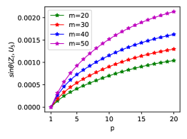
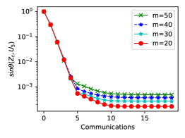
The final error depends on $m$. Big $m$ means smaller local sample size, $s=\frac{n}{m}$, and thereby big matrix approximation error, $\eta$ (in Definition 2). Our theory indicates that big $m$ (and thereby big $\eta$) is bad for the final error. The empirical results in Figure 3(c) corroborate our theories.

Table 1: We report the errors of three proposed algorithms and three baselines methods on seven datasets. We show the mean errors of ten repeated experiments with its standard deviation enclosed in parentheses. The result of full fifteen datasets is shown in Table 6.

Datasets	LocalPower $(p=4)$			DR-SVD	UDA	WDA
	OPT	Sign-fixing	Vanilla
A9a	4.09e-03 (4.20e-4)	5.82e-03 (1.41e-3)	8.13e-02 (3.44e-2)	4.63e-02 (9.24e-3)	2.64e-02 (1.58e-2)	2.40e-02 (1.50e-2)
Abalone	3.16e-03 (2.89e-3)	3.85e-03 (2.54e-3)	3.03e-02 (5.70e-2)	3.20e-01 (2.30e-1)	1.03e-01 (9.38e-2)	1.03e-01 (9.18e-2)
Acoustic	1.83e-03 (4.40e-4)	2.03e-03 (3.90e-4)	2.38e-03 (8.5e-4)	1.54e-02 (6.59e-3)	7.76e-03 (2.64e-3)	6.67e-03 (2.42e-3)
Combined	6.01e-03 (1.59e-3)	5.57e-03 (1.05e-3)	2.47e-02 (3.40e-2)	5.19e-02 (6.23e-3)	4.63e-02 (2.97e-3)	4.16e-02 (2.76e-2)
Connect-4	1.27e-02 (4.52e-3)	1.81e-02 (3.79e-3)	1.70e-02 (4.35e-3)	1.61e-02 (2.96e-3)	1.65e-01 (3.48e-2)	1.56e-0 1(3.26e-2)
Covtype	7.38e-03 (6.50e-4)	6.23e-03 (4.70e-4)	1.28e-02 (1.88e-3)	1.82e-01 (8.73e-2)	6.09e-02 (9.70e-3)	5.60e-02 (9.41e-3)
MSD	9.90e-03 (1.21e-3)	9.62e-03 (5.20e-4)	1.44e-02 (1.58e-3)	3.01e-02 (9.64e-3)	1.55e-02 (1.39e-3)	1.92e-02 (1.14e-3)

Table 2: Error comparison of LocalPower with decay strategy under the same setting of Table 1. See Table 7 for full results. In theory, LocalPower with decay strategy achieves zero error.

Datasets	LocalPower with $p=4$ and the decay strategy
	OPT	Sign-fixing	Vanilla
A9a	4.84e-03 (1.40e-02)	1.52e-03 (4.08e-03)	3.11e-04 (4.84e-04)
Abalone	3.50e-10 (4.10e-10)	4.14e-10 (4.00e-10)	6.12e-10 (6.77e-10)
Acoustic	1.40e-05 (2.16e-05)	1.92e-05 (3.72e-05)	2.28e-05 (4.91e-05)
Combined	3.68e-03 (5.63e-03)	7.74e-03 (1.70e-02)	2.99e-03 (3.88e-03)
Connect-4	4.90e-03 (8.47e-03)	3.58e-03 (4.35e-03)	3.09e-03 (3.16e-03)
Covtype	5.57e-04 (1.55e-03)	4.95e-05 (5.40e-05)	8.01e-05 (8.62e-05)
MSD	2.75e-05 (3.34e-05)	2.47e-05 (3.27e-05)	3.02e-05 (2.10e-05)

Table 3: The value of $\eta$ under uniform partitions on some datasets. It can be seen that for a fixed $n$, the larger $m$, the larger $\eta$. Full results see Table 5.

Dataset	$m=20$	$m=40$	$m=60$
A9a	0.034	0.0563	0.0701
Abalone	0.1089	0.23	0.2458
Acoustic	0.0063	0.0107	0.0134
Combined	0.006	0.0089	0.0113
Connect-4	0.0376	0.054	0.0771
Covtype	0.0078	0.011	0.0159
MSD	0.0007	0.0009	0.0012

Effect of local power iterations.

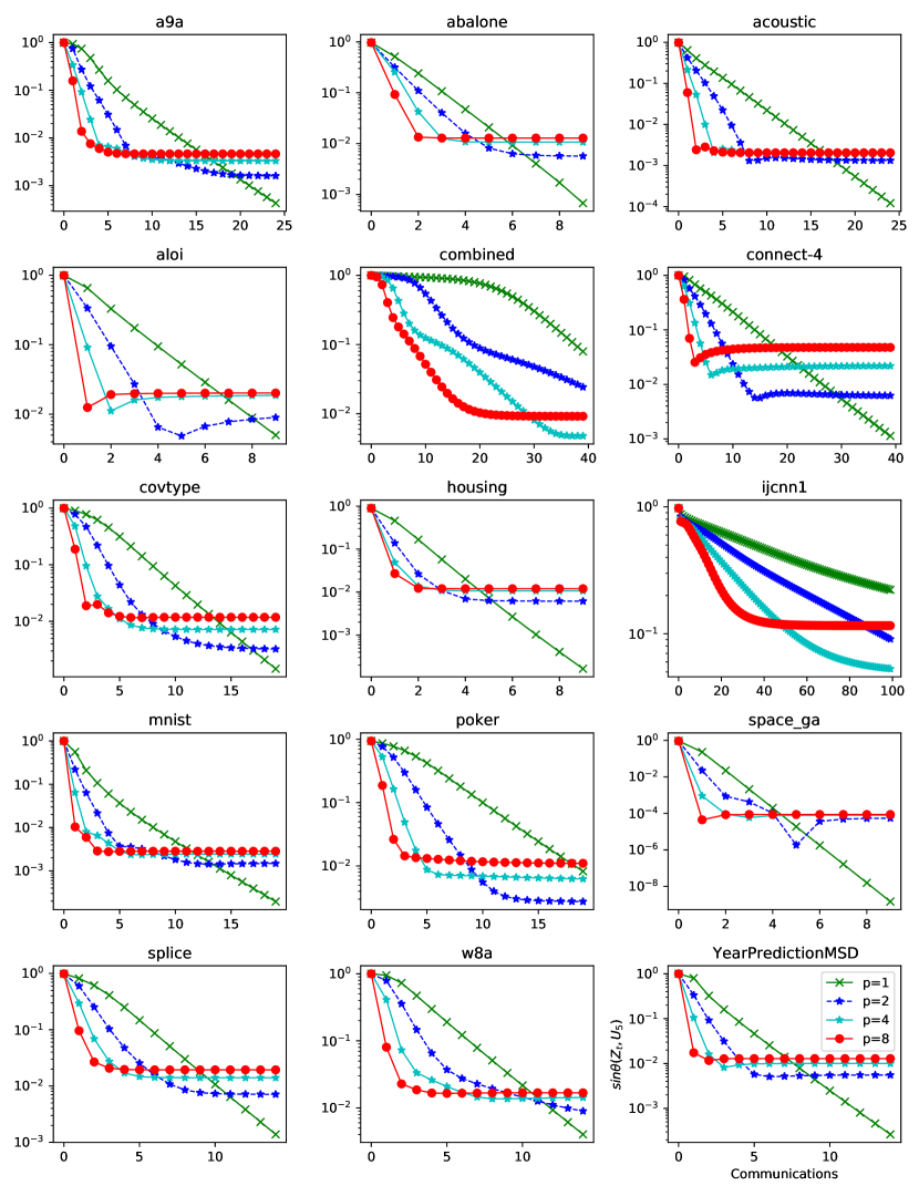
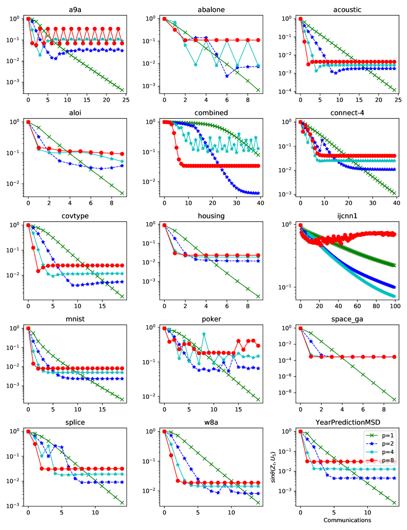
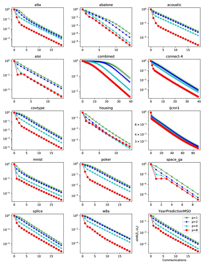
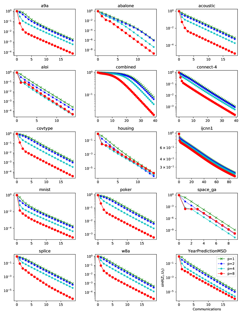
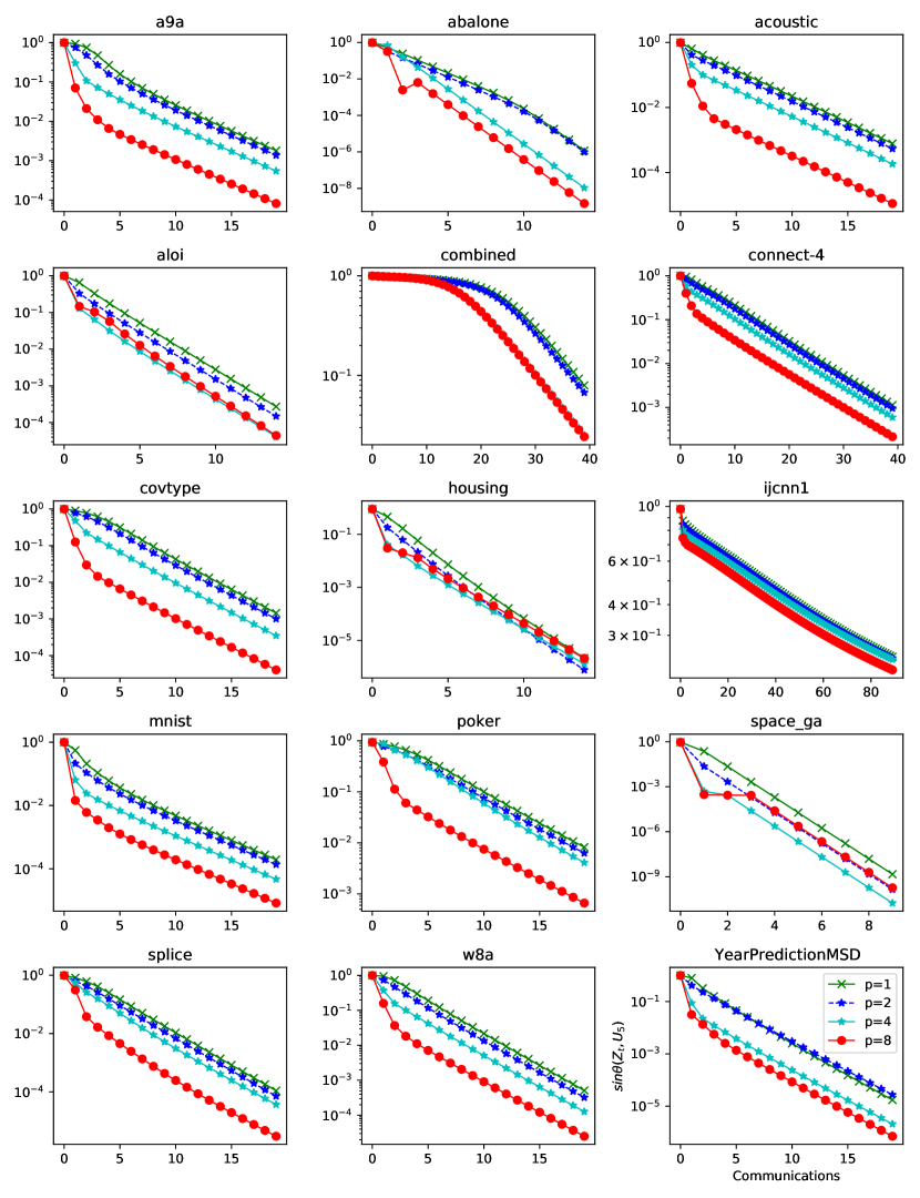
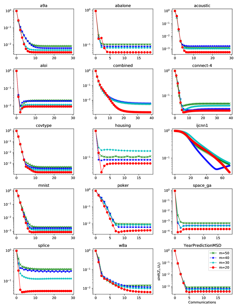
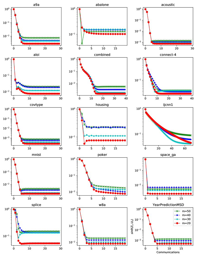
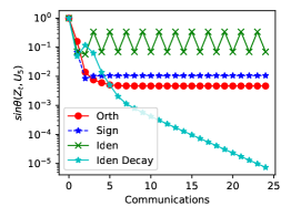
In this set of experiments, we set $p$ to $1$, $2$, $4$, or $8$ (without decaying $p$) and compare the convergence curves. Note that LocalPower with $p=1$ is the standard distributed power iteration (DPI). We plot the error, $\sin\theta_{k}({\bf Z}_{t},{\bf U}_{k})$, against communications. The convergence curves indicate how $p$ affects the communication efficiency. Figure 2(a) shows the experimental results on one dataset. Due to page limit, the results on the other datasets are left to the appendix; see Figures 5, 6, and 7. In all the experiments, large $p$ leads to fast convergence in the beginning but has a nonvanishing error in the end.

Some machine learning tasks, such as principal component analysis and latent semantic analysis [14], do not require high-precision solutions. In this case, LocalPower is advantageous over DPI, as LocalPower finds a satisfactory solution using very few communications. For two-stages methods like [19] It is also implied that LocalPower helps If a higher precision is required, we can decay $p$ so that LocalPower will have the same precision as DPI. While one-shot algorithms are more communication-efficient, their precision is too low unless each node has a large sample size.

The decay strategy.

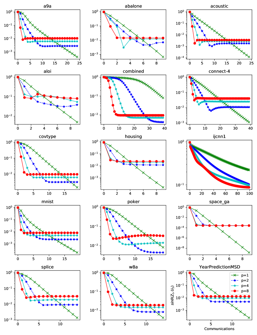
We have observed that large $p$ fastens initial convergence but enlarges the final error. By contrast, $p=1$ has the lowest error (which actually can be zero) but also the lowest convergence rate. Similar phenomena have been previously observed in distributed empirical risk minimization [47, 30]. To allow for both fast initial convergence and vanishing final error, we are motivated to decay $p$ gradually. We halve $p$ every iteration until it reaches $1$. We apply the decay strategy to the three variants of LocalPower. For each setting and each dataset, we repeat the experiment 10 times and report the mean and std. Table 3 and Figure 3(a) show the results on some datasets. The results on all the 15 datasets are left to the appendix; see Table 7, Figures 8, 9, and 10. The decay strategy not only makes convergence faster but also improves the final precision well.

Stability.

In almost all the experiments, LocalPower with OPT has smaller std and more stable convergence curves than LocalPower without OPT. Why does OPT improve stability. Theorem 2 shows that with OPT, $\rho_{t}$ (in Definition 3) has a linear function of $p$. Even if $p$ is large, Assumption 1 can be satisfied, and thus Theorem 1 guarantees the convergence of LocalPower with OPT. However, Theorem 2 shows that without using OPT, $\rho_{t}$ is an exponential function of $p$. If $p$ is large, Assumption 1 is violated, and thus the convergence of LocalPower without OPT is not guaranteed.

Sign-fixing is practical alternative to OPT. Table 1 and Figures 5 and 6 show that sign-fixing has comparable stability as OPT. To explain why sign-fixing works, we first explain what causes instability. Note that if we flip the signs of some columns of ${\bf Z}_{t}^{(i)}$, the subspace ${\mathcal{R}}({\bf Z}_{t}^{(i)})$ remains the same. During the local power iterations on the $i$-th node, the signs of the columns of ${\bf Z}_{t}^{(i)}$ can flip. While the sign flipping does not affect ${\mathcal{R}}({\bf Z}_{t}^{(i)})$, it changes the outcome of the aggregation of ${\bf Z}_{t}^{(1)},\cdots,{\bf Z}_{t}^{(m)}$. The sign-fixing method can counteract sign flippings and thereby stabilizes LocalPower.

Table 3 shows that LocalPower with decaying $p$ has better stability. With the decaying strategy used, $p$ will drop to $1$ after several communications, and LocalPower becomes the standard DPI which does not suffer from the instability issue.

(a) The performance of LocalPower with different $p$ on Covtype dataset

(b) Stability on A9a dataset

Figure 2: (a) We illustrate the convergence of LocalPower with different ${\mathcal{F}}$’s and various $p$ on Covtype dataset where ${\bf A}\in{\mathbb{R}}^{581,012\times 54}$. See Figure 5, 6 and 7 for full results. (b) The vanilla LocalPower sometimes fluctuates and even diverges (see Figure 7 for full results). We can stabilize it in two ways: (i) use ${\mathcal{O}}_{k}$ or ${\mathcal{D}}$ instead or (ii) use the decay strategy.

Effect of local sample size.

Since the $n$ data samples are partitioned among $m$ nodes uniformly at random, every node holds $s=\frac{n}{m}$ samples. Figure 3(b) shows that small $m$, equivalently, big $s$, is good for LocalPower. We use $\eta=\max_{i\in[m]}\|{\bf M}_{i}-{\bf M}\|_{2}/\|{\bf M}\|_{2}$ to measure the difference between a local covariance matrix and the full one. We give the values of $\eta$ under different uniform partitions in Table 3. It shows that if $s$ is large (so $m$ is small), $\eta$ is small, which implies ${\bf M}_{1},\cdots,{\bf M}_{m}$ well approximate the global matrix ${\bf M}$, and the residuals accumulated by the local iterations are small. It in turn makes the curves with small $m$ have small errors. This can be explained by our theories.

(a) Decay strategy

(b) Vary device number $m$

(c) Error dependence on $p$ and $m$

Figure 3: Some results on Covtype dataset. (a) A typical convergence curve of the decay strategy. See Figure 8, 9 and 10 for full results. (b) The smaller $m$, the faster convergence as well as the smaller error. See Figure 11 and 12 for full results. (c) The error depends positively on $p$ and $m$. See Figure 13 for full results.

6 Discussion

Smallness on $\eta$.

Theorem 1 requires $\eta={\mathcal{O}}(\frac{1}{\kappa})$ which might be too stringent in practice. If we use a refined analysis just like Guo et al. [24], it can be relaxed to $\eta={\mathcal{O}}({1})$ as well as $\epsilon_{0}$ whose dependence on $\kappa$ can be removed. Besides, the concurrent work [10] provides sharper analysis on one-shot average via OPT, which might be used to refine our analysis and relax the strictness on $\eta$ further.

Increase local sample size.

In addition to OPT or the decay strategy, we find that increasing local data size also reduces the final error. Intuitively, if $s_{i}$ is sufficiently large, then ${\bf M}_{i}=\frac{1}{s_{i}}{\bf A}_{i}^{\top}{\bf A}_{i}$ will be very close to ${\bf M}=\frac{1}{n}{\bf A}^{\top}{\bf A}$. Actually, this is true if we construct each ${\bf A}_{i}$ by sampling uniformly from the overall data ${\bf A}$ (see Lemma 2). Therefore, to make $\eta$ sufficiently small, we can increase local data size. If the total number of rows $n$ is fixed in advance, increasing each $s_{i}$ is equivalent to decreasing the number of worker nodes $m$.

The term $\eta=\max_{i\in[m]}\|{\bf M}_{i}-{\bf M}\|_{2}/\|{\bf M}\|_{2}$ is commonly used to analyze matrix approximation problems. It aims to ensure each ${\bf A}_{i}$ is a typical representative of the whole dataset ${\bf A}$. Prior work [20, 52, 49] showed that uniform sampling and the partition size in Lemma 2 suffice for that ${\bf M}_{i}$ well approximates ${\bf M}$. The proof is based on matrix Bernstein [45]. Therefore, under uniform sampling, the smallness of $\eta$ means sufficiently large local dataset size (or equivalently a small number of worker nodes). This can be also seen in Table 3.

One may doubt the motivation of each device anticipating the cooperated eigenspace estimation due to the large local dataset assumption. Here we focus on the empirical PCA rather than the population PCA. This implies we inevitably suffer a statistic error that will diminish if we have an infinite number of total samples. As a result, if $m$ devices participate in the training with comparable local data size, the statistical error can be reduced by a factor of $\sqrt{m}$. See Appendix B for more details.

Lemma 2 (Uniform sampling.).

Let $\epsilon,\delta\in(0,1)$. Assume the rows of ${\bf A}_{i}$ are sampled from the rows of ${\bf A}$ uniformly at random. Assume each node has sufficiently many samples, that is, for all $i\in m$,

$$s_{i}\geq\frac{3\mu\rho}{\epsilon^{2}}\log\big{(}\frac{\rho m}{{\delta}}\big{)},$$

where $\rho=\mathrm{rank}({\bf A})$ and $\mu$ is the row coherence of ${\bf A}$. With probability greater than $1-\delta$, we have

$$\eta=\max_{i\in[m]}\|{\bf M}_{i}-{\bf M}\|_{2}/\|{\bf M}\|_{2}\leq\epsilon.$$

Error dependence.

The choice of ${\mathcal{I}}_{T}$ determines the frequency LocalPower communicates. We explore the use of ${\mathcal{I}}_{T}=\{0,p,2p,\cdots,p\}$ and the decay strategy in experiments. When $p=1$, LocalPower reduces to DPI. As a result, both the residual errors $\varPsi_{t}$ and $\varOmega_{t}$ vanish. As shown in Lemma 1, DPI converges to zero error. When $p\geq 2$, the error $\sin\theta_{k}$ typically increases with $p$ and is non-zero. Corollary 1 depicts the relationship between the error and problem-dependent parameters including $n,m,p$. The proof is provided in Appendix A.5. It can be proved by Theorem 2 and Lemma 2.

Corollary 1.

Under uniform sampling and assuming $s_{i}=\Theta(\frac{n}{m})$ and $n$ is sufficiently large, , with probability 1- $\delta$, LocalPower with OPT has an asymptotic error satisfying

$$\limsup_{t\to\infty}\sin\theta_{k}({\bf Z}_{T},{\bf U}_{k})={\mathcal{O}}\left(h_{p}\left(\sqrt{\frac{m}{n}}\right)\right),$$

where $h_{p}(x)$ is non-negative and increasing in (typically both $p$ and) $x$, and it satisfies $h_{1}(x)=0$ as well as $0\leq h_{p}(x)\leq Cx$ for some $C$. We hide constants $\sigma_{k},k,d,\rho,\kappa,\delta$ in the big-${\mathcal{O}}$ notation and $h_{p}(\cdot)$. However, with any decay strategy in which $p$ converges to $1$ finally, LocalPower achieves zero error asymptotically.

Corollary 1 says that when $p$ goes to infinity, the error is saturated and has a finite limit, because $h_{p}(\cdot)$ is bounded. The curve of error v.s. $p$ and $m$ in Figure 3(c) validates the conclusion. Indeed, the extreme case of super large $p$ means LocalPower reduces to the one-shot method, which has a non-zero optimization error typically. Corollary 1 also reveals methods to reduce error. To that end, we can (i) use the decay strategy ($p\downarrow$) to achieve arbitrary error or (ii) reduce the number of devices ($m\downarrow$) or collect more data points $n\uparrow$. Both methods work in experiments empirically.

Dependence on $\sigma_{k}{-}\sigma_{k+1}$.

Our result depends on $\sigma_{k}{-}\sigma_{k+1}$ even when $r>k$ where $r$ is the number of columns used in subspace iteration. If we borrow the tool of Balcan et al. [4] rather than that of Hardt & Price [26], we can improve the result to a slightly milder dependency on $\sigma_{k}{-}\sigma_{q+1}$, where $q$ is any intermediate integer between $k$ and $r$. In particular, the required iteration $T$ will decrease from $\widetilde{{\mathcal{O}}}\left(\frac{\sigma_{k}}{\sigma_{k}-\sigma_{k+1}}\right)$ to $\widetilde{{\mathcal{O}}}\left(\frac{\sigma_{k}}{\sigma_{k}-\sigma_{q+1}}\right)$. It means using additional columns fastens convergence. For a formal statement, please refer to Appendix C.

Further extensions.

Our proposed LocalPower is simple, effective and well-grounded. While we analyze it only on the centralized setting, LocalPower can be extended to broader settings, such as decentralized setting [16] and streaming setting [35]. To further reduce the communication complexity, we can combine LocalPower with sketching techniques [7, 5]. For example, we could sketch each ${\bf Y}_{t}^{(i)}$ and communicate the compressed iterates to a central server in each iteration. We leave the extensions to our future work. Besides, in typical federated learning structures, real systems clients might not correspond to the central server due to connection failure. It is also possible to consider partial participation of clients and the optimal way of client selection [36, 11]. Guo et al. [24] makes an attempt towards the direction.

7 Conclusion

We have developed a communication-efficient distributed algorithm named LocalPower to solve the truncated SVD. Every worker machine performs multiple (say $p$) local power iterations between two consecutive communications. We have theoretically shown that LocalPower converges $p$ times faster (in terms of communication) than the baseline distributed power iteration, if the residual error is uniformly small. To reduce the residual error, we can (i) use OPT or sign-fixing, (ii) make use of a decay strategy that halves $p$ gradually, and (iii) increase local data size. Both OPT and sign-fixing are more stable, while sign-fixing additionally is computationally efficient. The strategy is motivated by an experimental phenomenon that large $p$ often leads to a quick initial drop of loss but a higher final error. The decay strategy obtains zero error asymptotically in theory and has better convergence performance in experiments. We have conducted the thorough experiments to show the effectiveness of LocalPower and all the theories are agree with our empirical experiments.

Appendix

Appendix A Proof for Section 4

A.1 Angles Between Two Equidimensional Subspaces

In this section, we introduce full definitions and lemmas on metrics between two subspaces, which will be useful in our following proof.

Principal Angles.

Given two matrices ${\bf U},{\widetilde{{\bf U}}}\in{\mathcal{O}}_{d\times k}$ which are both full rank with $1\leq k\leq d$, we define the $i$-th ($1\leq i\leq k$) principal angle between ${\bf U}$ and ${\widetilde{{\bf U}}}$ in a recursive manner:

$$\theta_{i}({\bf U},{\widetilde{{\bf U}}})=\min\bigg{\{}\arccos\left(\frac{{\bf x}^{\top}{\bf y}}{\|{\bf x}\|\|{\bf y}\|}\right):{\bf x}\in{\mathcal{R}}({\bf U}),{\bf y}\in{\mathcal{R}}({\widetilde{{\bf U}}}),{\bf x}\perp{\bf x}_{j},{\bf y}\perp{\bf y}_{j},\forall j<i\bigg{\}}$$ (7)

where ${\mathcal{R}}({\bf U})$ denotes by the space spanned by all columns of ${\bf U}$. In this definition, we require that $0\leq\theta_{1}\leq\cdots\leq\theta_{k}\leq\frac{\pi}{2}$ and that $\{{\bf x}_{1},\cdots,{\bf x}_{k}\}$ and $\{{\bf y}_{1},\cdots,{\bf y}_{k}\}$ are the associated principal vectors. Principal angles can be used to quantify the differences between two given subspaces.

We have following facts about the $k$-th principal angle between ${\bf U}$ and ${\widetilde{{\bf U}}}$:

Fact 1.

Let ${\bf U}^{\perp}$ denote by the complement subspace of ${\bf U}$ (so that $[{\bf U},{\bf U}^{\perp}]\in{\mathbb{R}}^{d\times d}$ forms an orthonormal basis of ${\mathbb{R}}^{d}$) and so dose ${\widetilde{{\bf U}}}^{\perp}$,

1. $\sin\theta_{k}({\bf U},{\widetilde{{\bf U}}})=\|{\bf U}^{\top}{\widetilde{{\bf U}}}^{\perp}\|=\|{\widetilde{{\bf U}}}^{\top}{\bf U}^{\perp}\|$;

2. $\tan\theta_{k}({\bf U},{\widetilde{{\bf U}}})=\|\left[({\bf U}^{\perp})^{\top}{\widetilde{{\bf U}}}\right]({\bf U}^{\top}{\widetilde{{\bf U}}})^{\dagger}\|$ where $\dagger$ denotes by the Moore–Penrose inverse.

3. For any reversible matrix ${\bf R}\in{\mathbb{R}}^{k\times k}$, $\tan\theta_{k}({\bf U},{\widetilde{{\bf U}}})=\tan\theta_{k}({\bf U},{\widetilde{{\bf U}}}{\bf R})$.

Projection Distance.

Define the projection distance between two subspaces by

$$\operatorname{dist}({\bf U},{\widetilde{{\bf U}}})=\|{\bf U}{\bf U}^{\top}-{\widetilde{{\bf U}}}{\widetilde{{\bf U}}}^{\top}\|.$$ (8)

This metric has several equivalent expressions:

$$\operatorname{dist}({\bf U},{\widetilde{{\bf U}}})=\|{\bf U}^{\top}{\widetilde{{\bf U}}}^{\perp}\|=\|{\widetilde{{\bf U}}}^{\top}{\bf U}^{\perp}\|=\sin\theta_{k}({\bf U},{\widetilde{{\bf U}}}).$$

More generally, for any two matrix ${\bf A},{\bf B}\in{\mathbb{R}}^{d\times k}$, we define the projection distance between them as

$$\operatorname{dist}({\bf A},{\bf B})=\|{\bf U}_{\bf A}{\bf U}_{\bf A}^{\top}-{\bf U}_{\bf B}{\bf U}_{\bf B}^{\top}\|$$

where ${\bf U}_{\bf A},{\bf U}_{\bf B}$ are the orthogonal basis of ${\mathcal{R}}({\bf A})$ and ${\mathcal{R}}({\bf B})$ respectively.

Orthogonal Procrustes.

Let ${\bf U},{\widetilde{{\bf U}}}\in{\mathbb{R}}^{d\times k}$ be two orthonormal matrices. ${\mathcal{R}}({\bf U})$ is close to ${\mathcal{R}}({\widetilde{{\bf U}}})$ does not necessarily imply ${\bf U}$ is close to ${\widetilde{{\bf U}}}$, since any orthonormal invariant of ${\bf U}$ forms a base of ${\mathcal{R}}({\bf U})$. However, the converse is true. If we try to map ${\widetilde{{\bf U}}}$ to ${\bf U}$ using an orthogonal transformation, we arrive at the following optimization

$${\bf O}^{*}=\mathop{\rm argmin}_{{\bf O}\in{\mathcal{O}}_{k}}\|{\bf U}-{\widetilde{{\bf U}}}{\bf O}\|_{F},$$ (9)

where ${\mathcal{O}}_{k}$ denotes the set of $k\times k$ orthogonal matrices. The following lemma shows there is an interesting relationship between the subspace distance and their corresponding basis matrices. It implies that as a metric on linear space, $\operatorname{dist}({\bf U},{\widetilde{{\bf U}}})$ is equivalent to $\|{\bf U}-{\widetilde{{\bf U}}}{\bf O}^{*}\|_{2}$ (or $\min_{{\bf O}\in{\mathcal{O}}_{k}}\|{\bf U}-{\widetilde{{\bf U}}}{\bf O}\|_{2}$) up to some universal constant. The optimization problem involved in is named as the orthogonal procrustes problem and has been well studied [38, 9].

Lemma 3.

Let ${\bf U},{\widetilde{{\bf U}}}\in{\mathcal{O}}_{d\times k}$ and ${\bf O}^{*}$ is the solution of eqn. (9). Then we have

1. ${\bf O}^{*}$ has a closed form given by ${\bf O}^{*}={\bf W}_{1}{\bf W}_{2}^{\top}$ where ${\widetilde{{\bf U}}}^{\top}{\bf U}={\bf W}_{1}\mbox{\boldmath$\Sigma$\unboldmath}{\bf W}_{2}^{\top}$ is the singular value decomposition of ${\widetilde{{\bf U}}}^{\top}{\bf U}$.

2. Define $d({\bf U},{\widetilde{{\bf U}}}):=\|{\bf U}-{\widetilde{{\bf U}}}{\bf O}^{*}\|_{2}$ where $\|\cdot\|_{2}$ is the spectral norm. Then we have

   $$d({\bf U},{\widetilde{{\bf U}}})=\sqrt{2-2\sqrt{1-\operatorname{dist}({\bf U},{\widetilde{{\bf U}}})^{2}}}=2\sin\frac{\theta_{k}({\bf U},{\widetilde{{\bf U}}})}{2}.$$

3. $d({\bf U}_{1},{\bf U}_{2})=d({\bf U}_{2},{\bf U}_{1})$ for any ${\bf U}_{1},{\bf U}_{2}\in{\mathcal{O}}_{d\times k}$.

4. $\operatorname{dist}({\bf U},{\widetilde{{\bf U}}})\leq d({\bf U},{\widetilde{{\bf U}}})\leq\sqrt{2}\operatorname{dist}({\bf U},{\widetilde{{\bf U}}})$.

5. Define

   $$\ell({\bf U},{\widetilde{{\bf U}}}):=\min_{{\bf O}\in{\mathcal{O}}_{k}}\|{\bf U}-{\widetilde{{\bf U}}}{\bf O}\|_{2}.$$

   Then $\ell({\bf U},{\widetilde{{\bf U}}})$ is a metric satisfying

   • $\ell({\bf U},{\widetilde{{\bf U}}})\geq 0$ for all ${\bf U},{\widetilde{{\bf U}}}\in{\mathcal{O}}_{d\times k}$. $\ell({\bf U},{\widetilde{{\bf U}}})=0$ if and only if ${\mathcal{R}}({\bf U})={\mathcal{R}}({\widetilde{{\bf U}}})$.

   • $\ell({\bf U},{\widetilde{{\bf U}}})=\ell({\widetilde{{\bf U}}},{\bf U})$ for all ${\bf U},{\widetilde{{\bf U}}}\in{\mathcal{O}}_{d\times k}$.

   • $\ell({\bf U}_{1},{\bf U}_{2})\leq\ell({\bf U}_{1},{\bf U}_{3})+\ell({\bf U}_{3},{\bf U}_{2})$ for any ${\bf U}_{1},{\bf U}_{2}$ and ${\bf U}_{3}\in{\mathcal{O}}_{d\times k}$.

6. $\frac{1}{\sqrt{k}}\operatorname{dist}({\bf U},{\widetilde{{\bf U}}})\leq\ell({\bf U},{\widetilde{{\bf U}}})\leq d({\bf U},{\widetilde{{\bf U}}})\leq\sqrt{2}\operatorname{dist}({\bf U},{\widetilde{{\bf U}}})$.

Proof.

The first item comes from Schönemann [38]. The second item comes from Cape [9]. The third and forth items follow from the second one. The fifth item follows directly from definition. For the rightest two $\leq$ of the last item, we use $\ell({\bf U},{\widetilde{{\bf U}}})\leq d({\bf U},{\widetilde{{\bf U}}})$ and the forth item. For the leftest $\leq$, we use $\min_{{\bf O}\in{\mathcal{O}}_{k}}\|{\bf U}-{\widetilde{{\bf U}}}{\bf O}\|_{2}\geq\frac{1}{\sqrt{k}}\min_{{\bf O}\in{\mathcal{O}}_{k}}\|{\bf U}-{\widetilde{{\bf U}}}{\bf O}\|_{F}$ and $\min_{{\bf O}\in{\mathcal{O}}_{k}}\|{\bf U}-{\widetilde{{\bf U}}}{\bf O}\|_{F}\geq\operatorname{dist}({\bf U},{\widetilde{{\bf U}}})$ (which is referred from Proposition 2.2 of Vu et al. [46]). ∎

A.2 Proof Technique and Useful Lemmas

Update Rule.

Assume $1=\mathop{\rm argmax}\limits_{i\in[m]}p_{i}$. We overwrite ${\bf Y}_{t}^{(i)}$ when $t\in{\mathcal{I}}_{T}$ (line 4 in Algorithm 1). To distinguish the difference, we additionally use ${\bf V}_{t}^{(i)}$ to denote the updated but not communicated ${\bf Y}_{t}^{(i)}$. Then the update rule becomes for all $i\in[m]$,

$${\bf V}_{t}^{(i)} ={\bf M}_{i}{\bf Z}_{t-1}^{(i)};$$ (10)

$${\bf Y}_{t}^{(i)} =\begin{cases}{\bf V}_{t}^{(i)}&\text{if}\ t\notin{\mathcal{I}}_{T};\\ \sum_{i=1}^{m}p_{i}{\bf V}_{t}^{(i)}{\bf D}_{t}^{(i)}&\text{if}\ t\in{\mathcal{I}}_{T}.\end{cases}$$ (11)

$${\bf Y}_{t}^{(i)} ={\bf Z}_{t}^{(i)}{\bf R}_{t}^{(i)}.$$ (12)

Here we abuse the notation a little bit and define ${\bf D}_{t}^{(i)}$ as

$${\bf D}_{t}^{(i)}=\mathop{\rm argmin}\limits_{{\bf D}\in{\mathcal{F}}\cap{\mathcal{O}}_{k}}\|{\bf Z}_{t-1}^{(i)}{\bf D}-{\bf Z}_{t-1}^{(1)}\|_{o}$$ (13)

where $\|\cdot\|_{o}$ can be set as either the Frobenius norm $\|\cdot\|_{F}$ or the spectrum norm $\|\cdot\|_{2}$, though in the body text we use only $\|\cdot\|_{F}$. There are some observations about the update rule:

1. If $t\notin{\mathcal{I}}_{T}$, we have ${\bf M}_{i}{\bf Z}_{t-1}^{(i)}={\bf V}_{t}^{(i)}={\bf Y}_{t}^{(i)}={\bf Z}_{t}^{(i)}{\bf R}_{t}^{(i)}$.

2. If $t\in{\mathcal{I}}_{T}$, we have ${\bf Y}_{t}^{(1)}=\cdots={\bf Y}_{t}^{(m)}=\sum_{i=1}^{m}p_{i}{\bf V}_{t}^{(i)}{\bf D}_{t}^{(i)}=\sum_{i=1}^{m}p_{i}{\bf M}_{i}{\bf Z}_{t-1}^{(i)}{\bf D}_{t}^{(i)}$ and thus ${\bf R}_{t}^{(1)}=\cdots={\bf R}_{t}^{(m)}$ and ${\bf Z}_{t}^{(1)}=\cdots={\bf Z}_{t}^{(m)}$. It implies that ${\bf D}_{t+1}^{(i)}={\bf I}_{k}$.

3. If ${\mathcal{F}}={\mathcal{O}}_{k}$, then ${\bf D}_{t}^{(i)}$ is the OPT we introduced in Section 4. If ${\mathcal{F}}={\mathcal{D}}_{k}$, then ${\bf D}_{t}^{(i)}$ is the sign-fixing. If ${\mathcal{F}}=\{{\bf I}_{k}\}$, then ${\bf D}_{t}^{(i)}$ is always equal to the identity matrix ${\bf I}_{k}$ and we arrive at the vanilla LocalPower. The unified view helps us give theoretical analysis in a unified way.

Virtual Sequence.

To analyze convergence of LocalPower, we define a virtual sequences defined as the weighted aggregation of local eigenvector matrices, i.e.,

$${\overline{\bf Y}}_{t}=\sum_{i=1}^{m}p_{i}{\bf Y}_{t}^{(i)}{\bf O}_{t}^{(i)}.$$ (14)

Here ${\bf O}_{t}^{(i)}\in{\mathbb{R}}^{k\times k}$ is defined as

$${\bf O}_{t}^{(i)}=\begin{cases}{\bf I}_{k}&\text{if}\ t\in{\mathcal{I}}_{T}\\ {\bf D}_{t}^{(i)}&\text{if}\ t\notin{\mathcal{I}}_{T}.\end{cases}$$

If $t\in{\mathcal{I}}_{T}$, ${\overline{\bf Y}}_{t}={\bf Y}_{t}^{(i)}$ for $i\in[m]$ and thus is obtainable. Otherwise, ${\overline{\bf Y}}_{t}$ is a shadow matrix facilitating analysis.

Recurrence Lemma.

Lemma 4 shows that we can express ${\overline{\bf Y}}_{t+1}$ as a linear transformation of ${\overline{\bf Y}}_{t}$. The resulting expression is similar to the iterates of the noisy power method proposed in [26], which motivates us to apply their technique to prove the main convergence of LocalPower. Lemma 4 holds for any invertible ${\bf R}_{t}\in{\mathbb{R}}^{k\times k}$. But, to guarantee convergence, we should carefully determine ${\bf R}_{t}$. In Lemma 8, we will give a particular expression of ${\bf R}_{t}$, which plays a crucial role in helping us to bound the noise term ${\bf G}_{t}$.

Lemma 4 (Recurrence).

For any invertible ${\bf R}_{t}\in{\mathbb{R}}^{k\times k}$, we have

$${\overline{\bf Y}}_{t+1}=\left({\bf M}{\overline{\bf Y}}_{t}+{\bf G}_{t}\right){\bf R}_{t}^{-1}$$ (15)

where ${\bf M}=\frac{1}{n}{\bf A}^{\top}{\bf A}\in{\mathbb{R}}^{d\times d}$ and

$${\bf G}_{t}={\bf H}_{t}+{\bf W}_{t}$$ (16)

with ${\bf H}_{t}=\sum_{i=1}^{m}p_{i}{\bf H}_{t}^{(i)}$ and ${\bf W}_{t}=\sum_{i=1}^{m}p_{i}{\bf W}_{t}^{(i)}$. Here for $i\in[m]$,

$${\bf H}_{t}^{(i)}=\left({\bf M}_{i}-{\bf M}\right){\bf Y}_{t}^{(i)}{\bf O}_{t}^{(i)}\quad\text{and}\quad{\bf W}_{t}^{(i)}={\bf V}_{t+1}^{(i)}\left[{\bf D}_{t+1}^{(i)}{\bf R}_{t}-{\bf R}_{t}^{(i)}{\bf O}_{t}^{(i)}\right].$$ (17)

Proof.

First notice that we always have ${\overline{\bf Y}}_{t}=\sum_{i=1}^{m}p_{i}{\bf V}_{t}^{(i)}{\bf D}_{t}^{(i)}$. If $t\in{\mathcal{I}}_{T}$, ${\bf Y}_{t}^{(1)}=\cdots={\bf Y}_{t}^{(m)}$ and ${\bf O}_{t}^{(i)}={\bf I}_{r}$, implying the equation follows from eqn. (11) and eqn. (14). Otherwise, we have ${\bf Y}_{t}^{(i)}={\bf V}_{t}^{(i)}$ and ${\bf O}_{t}^{(i)}={\bf D}_{t}^{(i)}$, then ${\overline{\bf Y}}_{t}=\sum_{i=1}^{m}p_{i}{\bf Y}_{t}^{(i)}{\bf O}_{t}^{(i)}=\sum_{i=1}^{m}p_{i}{\bf V}_{t}^{(i)}{\bf D}_{t}^{(i)}$.

We always have ${\bf V}_{t+1}^{(i)}={\bf M}_{i}{\bf Z}_{t}^{(i)}={\bf M}_{i}{\bf Y}_{t}^{(i)}({\bf R}_{t}^{(i)})^{-1}$. Then for any invertible ${\bf R}_{t}$, we have

$${\overline{\bf Y}}_{t+1} =\sum_{i=1}^{m}p_{i}{\bf V}_{t+1}^{(i)}{\bf D}_{t+1}^{(i)}$$

$$=\sum_{i=1}^{m}p_{i}{\bf M}_{i}{\bf Y}_{t}^{(i)}({\bf R}_{t}^{(i)})^{-1}{\bf D}_{t+1}^{(i)}$$

$$=\sum_{i=1}^{m}p_{i}{\bf M}_{i}{\bf Y}_{t}^{(i)}{\bf O}_{t}^{(i)}{\bf R}_{t}^{-1}+\sum_{i=1}^{m}p_{i}{\bf M}_{i}{\bf Y}_{t}^{(i)}({\bf R}_{t}^{(i)})^{-1}\left[{\bf D}_{t+1}^{(i)}{\bf R}_{t}-{\bf R}_{t}^{(i)}{\bf O}_{t}^{(i)}\right]{\bf R}_{t}^{-1}$$

$$\overset{(a)}{=}\sum_{i=1}^{m}p_{i}\left({\bf M}{\bf Y}_{t}^{(i)}{\bf O}_{t}^{(i)}+{\bf H}_{t}^{(i)}\right){\bf R}_{t}^{-1}+\sum_{i=1}^{m}p_{i}{\bf M}_{i}{\bf Z}_{t}^{(i)}\left[{\bf D}_{t+1}^{(i)}{\bf R}_{t}-{\bf R}_{t}^{(i)}{\bf O}_{t}^{(i)}\right]{\bf R}_{t}^{-1}$$

$$=\sum_{i=1}^{m}p_{i}\left({\bf M}{\bf Y}_{t}^{(i)}{\bf O}_{t}^{(i)}+{\bf H}_{t}^{(i)}\right){\bf R}_{t}^{-1}+\sum_{i=1}^{m}p_{i}{\bf M}_{i}{\bf Z}_{t}^{(i)}\left[{\bf D}_{t+1}^{(i)}{\bf R}_{t}-{\bf R}_{t}^{(i)}{\bf O}_{t}^{(i)}\right]{\bf R}_{t}^{-1}$$

$$\overset{(b)}{=}\left({\bf M}{\overline{\bf Y}}_{t}+{\bf H}_{t}+{\bf W}_{t}\right){\bf R}_{t}^{-1}$$

where (a) results from the definition of ${\bf H}_{t}^{(i)}$; and (b) simplifies the equation via defining ${\bf H}_{t}=\sum_{i=1}^{m}p_{i}{\bf H}_{t}^{(i)}$ and ${\bf W}_{t}=\sum_{i=1}^{m}p_{i}{\bf W}_{t}^{(i)}$. Setting ${\bf G}_{t}={\bf H}_{t}+{\bf W}_{t}$ completes the proof.

∎

Convergence Lemma.

The following lemma is an variant of Lemma 2.2 in Hardt & Price [26]. Given the relation ${\overline{\bf Y}}_{t+1}=\left({\bf M}{\overline{\bf Y}}_{t}+{\bf G}_{t}\right){\bf R}_{t}^{-1}$, Hardt & Price [26] requires ${\overline{\bf Y}}_{t}$ to have orthonormal columns, i.e., ${\overline{\bf Y}}_{t}^{\top}{\overline{\bf Y}}_{t}={\bf I}_{r}$. However, it is unlikely to hold in our case. As a remedy, we slightly change the lemma to allow arbitrary ${\overline{\bf Y}}_{t}$. This will also change the condition on ${\bf G}_{t}$.

Lemma 5.

Let ${\bf U}_{k}\in{\mathbb{R}}^{d\times k}$ be the top-$k$ eigenvectors of a positive semi-definite matrix ${\bf M}$. For $t\geq 1$, assume ${\overline{\bf Y}}_{t}$ satisfies eqn. (15) and ${\bf G}_{t}\in{\mathbb{R}}^{d\times k}$ satisfy

$$4\|{\bf U}_{k}^{\top}{\bf G}_{t}{\overline{\bf Y}}_{t}^{\dagger}\|_{2}\leq(\sigma_{k}-\sigma_{k+1})\cos\theta_{k}\left({\bf U}_{k},{\overline{\bf Y}}_{t}\right)\quad\text{and}\quad 4\|{\bf G}_{t}{\overline{\bf Y}}_{t}^{\dagger}\|_{2}\leq(\sigma_{k}-\sigma_{k+1})\epsilon$$ (18)

where ${\overline{\bf Y}}_{t}^{\dagger}$ is the Moore–Penrose inverse of ${\overline{\bf Y}}_{t}$ and $\epsilon<1$. Then

$$\tan\theta_{k}\left({\bf U}_{k},{\overline{\bf Y}}_{t+1}\right)\leq\max\left(\epsilon,\max\left(\epsilon,\left(\frac{\sigma_{k+1}}{\sigma_{k}}\right)^{1/4}\right)\tan\theta_{k}\left({\bf U}_{k},{\overline{\bf Y}}_{t}\right)\right).$$

Proof.

Let ${\overline{\bf Y}}_{t}={\overline{\bf Z}}_{t}{\overline{\bf R}}_{t}$ be the QR factorization of ${\overline{\bf Y}}_{t}$ so that ${\overline{\bf Z}}_{t}$ has orthonormal columns. The recurrence relation becomes ${\overline{\bf Y}}_{t+1}=\left({\bf M}{\overline{\bf Z}}_{t}{\overline{\bf R}}_{t}+{\bf G}_{t}\right){\bf R}_{t}^{-1}=\left({\bf M}{\overline{\bf Z}}_{t}+{\bf G}_{t}{\overline{\bf R}}_{t}^{-1}\right){\overline{\bf R}}_{t}{\bf R}_{t}^{-1}$. By the fact 1, we have $\tan\theta_{k}\left({\bf U}_{k},{\overline{\bf Y}}_{t+1}\right)=\tan\theta_{k}\left({\bf U}_{k},{\overline{\bf Y}}_{t+1}{\bf R}_{t}{\overline{\bf R}}_{t}^{-1}\right)=\tan\theta_{k}\left({\bf U}_{k},{\bf M}{\overline{\bf Z}}_{t}+{\bf G}_{t}{\overline{\bf R}}_{t}^{-1}\right)$. By requiring

$$4\|{\bf U}_{k}^{\top}{\bf G}_{t}{\overline{\bf R}}_{t}^{-1}\|_{2}\leq(\sigma_{k}-\sigma_{k+1})\cos\theta_{k}\left({\bf U}_{k},{\overline{\bf Z}}_{t}\right)\quad\text{and}\quad 4\|{\bf G}_{t}{\overline{\bf R}}_{t}^{-1}\|_{2}\leq(\sigma_{k}-\sigma_{k+1})\epsilon,$$

we have from Lemma 2.2 in Hardt & Price [26] that

$$\tan\theta_{k}\left({\bf U}_{k},{\overline{\bf Y}}_{t+1}\right)\leq\max\left(\epsilon,\max\left(\epsilon,\left(\frac{\sigma_{k+1}}{\sigma_{k}}\right)^{1/4}\right)\tan\theta_{k}\left({\bf U}_{k},{\overline{\bf Z}}_{t}\right)\right).$$

Noting that ${\mathcal{R}}({\overline{\bf Y}}_{t})={\mathcal{R}}({\overline{\bf Z}}_{t})$, we have $\theta_{k}\left({\bf U}_{k},{\overline{\bf Y}}_{t}\right)=\theta_{k}\left({\bf U}_{k},{\overline{\bf Z}}_{t}\right)$ and thus

$$\cos\theta_{k}\left({\bf U}_{k},{\overline{\bf Y}}_{t}\right)=\cos\theta_{k}\left({\bf U}_{k},{\overline{\bf Z}}_{t}\right)\quad\text{and}\quad\tan\theta_{k}\left({\bf U}_{k},{\overline{\bf Y}}_{t}\right)=\tan\theta_{k}\left({\bf U}_{k},{\overline{\bf Z}}_{t}\right).$$

Finally, using $\|{\bf U}_{k}^{\top}{\bf G}_{t}{\overline{\bf Y}}_{t}^{\dagger}\|_{2}=\|{\bf U}_{k}^{\top}{\bf G}_{t}{\overline{\bf R}}_{t}^{-1}\|_{2}$ and $\|{\bf G}_{t}{\overline{\bf Y}}_{t}^{\dagger}\|_{2}=\|{\bf G}_{t}{\overline{\bf R}}_{t}^{-1}\|_{2}$ completes the proof.

∎

Other Useful Lemma.

Lemma 6 handles $\tan\theta_{k}({\bf U},{\bf Z}_{0})$ with randomly generate ${\bf Z}_{0}$, while Lemma 7 give a upper bound of $\|{\overline{\bf Y}}_{t}^{\dagger}{\bf M}\|_{2}$.

Lemma 6 (Lemma 2.4 in Hardt & Price [26]).

For an arbitrary orthonormal ${\bf U}$ and random subspace ${\bf Z}_{0}\in{\mathbb{R}}^{d\times r}$, with probability grater than $1-\tau^{-\Omega(r+1-k)}-e^{-\Omega(d)}$, we have that

$$\tan\theta_{k}({\bf U},{\bf Z}_{0})\leq\frac{\tau\sqrt{d}}{\sqrt{r}-\sqrt{k-1}}.$$

Lemma 7.

Recall that $\kappa=\|{\bf M}\|_{2}\|{\bf M}^{\dagger}\|_{2}$ and $\eta=\max_{i\in[m]}\|{\bf M}_{i}-{\bf M}\|_{2}/\|{\bf M}\|_{2}$. Define

$$\mu_{t}=1-\eta{\kappa}-\sum_{j=1}^{m}p_{j}\|{\bf Z}_{t-1}^{(j)}{\bf D}_{t}^{(j)}-{\bf Z}_{t-1}^{(1)}\|_{2}$$

and assume $\mu_{t}>0$. Then it follows that $\|{\overline{\bf Y}}_{t}^{\dagger}{\bf M}\|_{2}\leq\frac{1}{\mu_{t}}$.

Proof.

For any matrix ${\bf X}\in{\mathbb{R}}^{d\times k}$, we have

$$\|{\bf X}^{\dagger}\|_{2}=\max_{{\bf x}\in{\mathbb{R}}^{k}}\frac{\|{\bf w}\|_{2}}{\|{\bf X}{\bf w}\|_{2}}=\max_{\|{\bf X}{\bf w}\|_{2}=1}\|{\bf w}\|_{2}=\max\{\|{\bf w}\|_{2}:\|{\bf X}{\bf w}\|_{2}\leq 1\}.$$

Notice that ${\overline{\bf Y}}_{t}^{\dagger}{\bf M}=({\bf M}^{\dagger}{\overline{\bf Y}}_{t})^{\dagger}$ and ${\overline{\bf Y}}_{t}=\sum_{j=1}^{m}p_{j}{\bf M}_{j}{\bf Z}_{t-1}^{(j)}{\bf D}_{t}^{(j)}$. We then have

$$\|{\overline{\bf Y}}_{t}^{\dagger}{\bf M}\|_{2} =\|({\bf M}^{\dagger}{\overline{\bf Y}}_{t})^{\dagger}\|_{2}$$

$$=\max\{\|{\bf w}\|_{2}:\|{\bf M}^{\dagger}{\overline{\bf Y}}_{t}{\bf w}\|_{2}\leq 1\}$$

$$=\max\{\|{\bf w}\|_{2}:\|({\bf M}^{\dagger}\sum_{j=1}^{m}p_{j}{\bf M}_{j}{\bf Z}_{t-1}^{(j)}{\bf D}_{t}^{(j)}){\bf w}\|_{2}\leq 1\}$$

$$\overset{(a)}{\leq}\max\{\|{\bf w}\|_{2}:\|\sum_{j=1}^{m}p_{j}{\bf Z}_{t-1}^{(j)}{\bf D}_{t}^{(j)}{\bf w}\|_{2}-\eta\kappa\|{\bf w}\|_{2}\leq 1\}$$

$$\overset{(b)}{\leq}\max\{\|{\bf w}\|_{2}:\|{\bf w}\|_{2}(1-\eta\kappa-\sum_{j=1}^{m}p_{j}\|{\bf Z}_{t-1}^{(j)}{\bf D}_{t}^{(j)}-{\bf Z}_{t-1}^{(1)}\|_{2})\leq 1\}$$

$$\leq\frac{1}{1-\eta\kappa-\sum_{j=1}^{m}p_{j}\|{\bf Z}_{t-1}^{(j)}{\bf D}_{t}^{(j)}-{\bf Z}_{t-1}^{(1)}\|_{2}}\leq\frac{1}{\mu_{t}}$$

where (a) follows because of

$$\|({\bf M}^{\dagger}\sum_{j=1}^{m}p_{j}{\bf M}_{j}{\bf Z}_{t-1}^{(j)}{\bf D}_{t}^{(j)}){\bf w}\|_{2}\geq\|\sum_{j=1}^{m}p_{j}{\bf Z}_{t-1}^{(j)}{\bf D}_{t}^{(j)}{\bf w}\|_{2}-\sum_{i=1}^{m}p_{i}\|{\bf M}^{\dagger}({\bf M}_{j}-{\bf M})\|_{2}\|{\bf Z}_{t-1}^{(j)}{\bf D}_{t}^{(j)}{\bf w}\|_{2}$$

and $\|{\bf M}^{\dagger}({\bf M}_{j}-{\bf M})\|_{2}\leq\|{\bf M}^{\dagger}\|_{2}\|({\bf M}_{j}-{\bf M})\|_{2}\leq\eta\kappa$; and (b) holds since

$$\|\sum_{j=1}^{m}p_{j}{\bf Z}_{t-1}^{(j)}{\bf D}_{t}^{(j)}{\bf w}\|_{2} \geq\|\sum_{j=1}^{m}p_{j}{\bf Z}_{t-1}^{(1)}{\bf w}\|_{2}-\|\sum_{j=1}^{m}p_{j}({\bf Z}_{t-1}^{(j)}{\bf D}_{t}^{(j)}-{\bf Z}_{t-1}^{(1)}){\bf w}\|_{2}$$

$$\geq\|{\bf w}\|_{2}-\sum_{j=1}^{m}p_{j}\|{\bf Z}_{t-1}^{(j)}{\bf D}_{t}^{(j)}-{\bf Z}_{t-1}^{(1)}\|_{2}\|{\bf w}\|_{2}$$

$$=\|{\bf w}\|_{2}(1-\sum_{j=1}^{m}p_{j}\|{\bf Z}_{t-1}^{(j)}{\bf D}_{t}^{(j)}-{\bf Z}_{t-1}^{(1)}\|_{2}).$$

∎

A.3 The Choice of ${\bf R}_{t}$

In this section, we specify the choice of ${\bf R}_{t}$ and analyze the residual error bound $\|{\bf D}_{t+1}^{(i)}{\bf R}_{t}-{\bf R}_{t}^{(i)}{\bf O}_{t}^{(i)}\|_{2}$. Lemma 8 specifies the way we set ${\bf R}_{t}$. Given a baseline data matrix ${\bf M}_{o}$, ${\bf R}_{t}$ is the shadow matrix that depicts what the upper triangle matrix ought to be, if we start from the nearest synchronized matrix and perform QR factorization using the matrix ${\bf M}_{o}$. We will set ${\bf M}_{o}={\bf M}_{t}^{(1)}$ (by assuming $1=\mathop{\rm argmax}\limits_{i\in[m]}p_{i}$) and analyze $\|{\bf W}_{t}^{(i)}{\overline{\bf Y}}_{t}^{\dagger}\|_{2}$ and $\|{\bf H}_{t}^{(i)}{\overline{\bf Y}}_{t}^{\dagger}\|_{2}$ in terms of $\|{\bf Z}_{t}^{(i)}{\bf D}_{t+1}^{(i)}-{\bf Z}_{t}^{(1)}\|_{2}$. Latter we will bound $\|{\bf Z}_{t}^{(i)}{\bf D}_{t+1}^{(i)}-{\bf Z}_{t}^{(1)}\|_{2}$ when ${\mathcal{F}}$ is differently set.

Lemma 8 (Choice of ${\bf R}_{t}$).

Fix any $t$ and let $t_{0}=\tau(t)\in{\mathcal{I}}_{T}$ be the latest synchronization step before $t$, then $t\geq\tau(t)$.

• If $t=t_{0}$, we define ${\bf R}_{t}={\bf R}_{t}^{(i)}$ for any $i\in[m]$ since all ${\bf R}_{t}^{(i)}$’s are equal.

• If $t>t_{0}$, given a baseline data matrix ${\bf M}_{o}$, we define ${\bf R}_{t}\in{\mathbb{R}}^{r\times r}$ recursively as the following. Let ${\bf Y}_{t_{0}}={\overline{\bf Y}}_{t_{0}}={\bf Z}_{t_{0}}{\bf R}_{t_{0}}$, and for $l=t_{0},t_{0}+1,\cdots,t$, we use the following QR factorization to define ${\bf R}_{t}$’s:

  $${\bf V}_{l+1}={\bf M}_{o}{\bf Z}_{l}={\bf Z}_{l+1}{\bf R}_{l+1}.$$

Then for any $i\in[m]$, we have

$$\|{\bf D}_{t+1}^{(i)}{\bf R}_{t}-{\bf R}_{t}^{(i)}{\bf O}_{t}^{(i)}\|_{2}\leq\sigma_{1}({\bf M}_{o})\|{\bf Z}_{t}^{(i)}{\bf D}_{t+1}^{(i)}-{\bf Z}_{t}\|_{2}+\left[\|{\bf M}_{o}-{\bf M}_{i}\|_{2}+\sigma_{1}({\bf M}_{i})\|{\bf Z}_{t-1}^{(i)}{\bf D}_{t}^{(i)}-{\bf Z}_{t-1}\|_{2}\right]1_{t\notin{\mathcal{I}}_{T}}.$$ (19)

Proof.

We are going to bound $\|{\bf D}_{t+1}^{(i)}{\bf R}_{t}-{\bf R}_{t}^{(i)}{\bf O}_{t}^{(i)}\|_{2}$ in two cases depending on whether $t\in{\mathcal{I}}_{T}$. If $t\in{\mathcal{I}}_{T}$, implying $t=t_{0}:=\tau(u)$, then ${\bf O}_{t}^{(i)}={\bf D}_{t+1}^{(i)}={\bf I}_{r}$ and ${\bf R}_{t}={\bf R}_{t}^{(i)}$. Therefore, ${\bf D}_{t+1}^{(i)}{\bf R}_{t}-{\bf R}_{t}^{(i)}{\bf O}_{t}^{(i)}={\bf 0}$.

Otherwise, $t\notin{\mathcal{I}}_{T}$ and thus $t>t_{0}$. Let’s fix some $i\in[m]$ and denote $\Delta{\bf M}={\bf M}_{i}-{\bf M}_{o}$. Based on LocalPower, we have ${\bf Y}_{t_{0}}^{(i)}={\overline{\bf Y}}_{t_{0}}={\bf Z}_{t_{0}}^{(i)}{\bf R}_{t_{0}}^{(i)},$ and for $l=t_{0},t_{0}+1,\cdots,t$,

$${\bf V}_{l+1}^{(i)}={\bf M}_{i}{\bf Z}_{l}^{(i)}={\bf Z}_{l+1}^{(i)}{\bf R}_{t+1}^{(i)}.$$

Then,

$${\bf Z}_{l}^{(i)}{\bf R}_{l}^{(i)}{\bf O}_{l}^{(i)} ={\bf M}_{i}{\bf Z}_{l-1}^{(i)}{\bf O}_{l}^{(i)}$$

$$=({\bf M}_{o}+\Delta{\bf M})({\bf Z}_{l-1}+\Delta{\bf Z}_{l-1})$$

$$={\bf M}_{o}{\bf Z}_{l-1}+\Delta{\bf M}\cdot{\bf Z}_{l-1}+{\bf M}_{i}\cdot\Delta{\bf Z}_{l-1}$$

$$:={\bf M}_{o}{\bf Z}_{l-1}+{\bf E}_{l-1}={\bf Z}_{l}{\bf R}_{l}+{\bf E}_{l-1}$$

where ${\bf E}_{l-1}=\Delta{\bf M}\cdot{\bf Z}_{l-1}+{\bf M}_{i}\cdot\Delta{\bf Z}_{l-1}$ and $\Delta{\bf Z}_{l-1}={\bf Z}_{l-1}^{(i)}{\bf O}_{l}^{(i)}-{\bf Z}_{l-1}$.

Note that

$${\bf Z}_{t}^{(i)}{\bf R}_{t}^{(i)}{\bf O}_{t}^{(i)}={\bf Z}_{t}{\bf R}_{t}+{\bf E}_{t-1}.$$

Then we have

$$\|{\bf D}_{t+1}^{(i)}{\bf R}_{t}-{\bf R}_{t}^{(i)}{\bf O}_{t}^{(i)}\|_{2} =\|{\bf Z}_{t}^{(i)}{\bf D}_{t+1}^{(i)}{\bf R}_{t}-{\bf Z}_{t}^{(i)}{\bf R}_{t}^{(i)}{\bf O}_{t}^{(i)}\|_{2}$$

$$\overset{(a)}{=}\|{\bf Z}_{t}^{(i)}{\bf D}_{t+1}^{(i)}{\bf R}_{t}-{\bf Z}_{t}{\bf R}_{t}-{\bf E}_{t-1}\|_{2}$$

$$\leq\|({\bf Z}_{t}^{(i)}{\bf D}_{t+1}^{(i)}-{\bf Z}_{t}){\bf R}_{t}\|_{2}+\|{\bf E}_{t-1}\|_{2}$$

$$\overset{(b)}{\leq}\|{\bf Z}_{t}^{(i)}{\bf D}_{t+1}^{(i)}-{\bf Z}_{t}\|_{2}\|{\bf R}_{t}\|_{2}+\|\Delta{\bf M}\|_{2}+\|{\bf M}_{i}\|_{2}\|{\bf Z}_{t-1}^{(i)}{\bf O}_{t}^{(i)}-{\bf Z}_{t-1}\|_{2}$$

$$\overset{(c)}{\leq}\sigma_{1}({\bf M}_{o})\|{\bf Z}_{t}^{(i)}{\bf D}_{t+1}^{(i)}-{\bf Z}_{t}\|_{2}+\|{\bf M}_{o}-{\bf M}_{i}\|_{2}+\sigma_{1}({\bf M}_{i})\|{\bf Z}_{t-1}^{(i)}{\bf D}_{t}^{(i)}-{\bf Z}_{t-1}\|_{2}$$

where (a) uses the equality of ${\bf Z}_{t}^{(i)}{\bf R}_{t}^{(i)}{\bf O}_{t}^{(i)}$; (b) uses the definition of ${\bf E}_{t-1}$ and ${\bf O}_{t}^{(i)}={\bf D}_{t}^{(i)}$ (due to $t\notin{\mathcal{I}}_{T}$); and (c) uses $\|{\bf R}_{t}\|_{2}\leq\|{\bf M}_{o}\|_{2}=\sigma_{1}({\bf M}_{o})$.

Combining the two cases, we have for all $t\in[T]$,

$$\|{\bf D}_{t+1}^{(i)}{\bf R}_{t}-{\bf R}_{t}^{(i)}{\bf O}_{t}^{(i)}\|_{2}\leq\sigma_{1}({\bf M}_{o})\|{\bf Z}_{t}^{(i)}{\bf D}_{t+1}^{(i)}-{\bf Z}_{t}\|_{2}+\left[\|{\bf M}_{o}-{\bf M}_{i}\|_{2}+\sigma_{1}({\bf M}_{i})\|{\bf Z}_{t-1}^{(i)}{\bf D}_{t}^{(i)}-{\bf Z}_{t-1}\|_{2}\right]1_{t\notin{\mathcal{I}}_{T}}.$$

∎

Lemma 9.

Assume $\eta=\max_{i\in[m]}\|{\bf M}_{i}-{\bf M}\|_{2}/\|{\bf M}\|_{2}$ is sufficiently small and $1=\mathop{\rm argmax}\limits_{i\in[m]}p_{i}$. Define

$$\rho_{t}=\|{\bf Z}_{t}^{(i)}{\bf D}_{t+1}^{(i)}-{\bf Z}_{t}^{(1)}\|_{2},$$

we have

$$\|{\bf H}_{t}{\overline{\bf Y}}_{t}^{\dagger}\|_{2}\leq\frac{2\sigma_{1}\eta\kappa 1_{t\notin{\mathcal{I}}_{T}}}{1-\eta{\kappa}-(1-\max_{i\in[m]}p_{i})\rho_{t-1}}$$ (20)

$$\|{\bf W}_{t}{\overline{\bf Y}}_{t}^{\dagger}\|_{2}\leq 4(1-\max_{i\in[m]}p_{i})\sigma_{1}\kappa\frac{\rho_{t}+(\rho_{t-1}+\eta)1_{t\notin{\mathcal{I}}_{T}}}{1-\eta{\kappa}-(1-\max_{i\in[m]}p_{i})\rho_{t-1}}.$$ (21)

Proof.

Without loss of generality, we assume $1=\mathop{\rm argmax}\limits_{i\in[m]}p_{i}$ and then set the baseline matrix in Lemma 8 as ${\bf M}_{o}={\bf M}_{1}$ and use the ${\bf R}_{t}$ defined therein. Then Lemma 8 and Lemma 10 imply for all $i\in[m]$,

$$\|{\bf D}_{t+1}^{(i)}{\bf R}_{t}-{\bf R}_{t}^{(i)}{\bf O}_{t}^{(i)}\|_{2} \leq\sigma_{1}({\bf M}_{o})\|{\bf Z}_{t}^{(i)}{\bf D}_{t+1}^{(i)}-{\bf Z}_{t}\|_{2}+[\|{\bf M}_{o}-{\bf M}_{i}\|_{2}+\sigma_{1}({\bf M}_{i})\|{\bf Z}_{t-1}^{(i)}{\bf D}_{t}^{(i)}-{\bf Z}_{t-1}\|_{2}]1_{t\notin{\mathcal{I}}_{T}}$$

$$\leq(1+\eta)\sigma_{1}\left[\rho_{t}+\rho_{t-1}1_{t\notin{\mathcal{I}}_{T}}\right]+\eta\sigma_{1}1_{i\neq 1\ \text{and}\ t\notin{\mathcal{I}}_{T}}$$

where $\sigma_{1}=\sigma_{1}({\bf M})$ and $1_{i\neq 1\ \text{and}\ t\notin{\mathcal{I}}_{T}}$ is the indicator of event $\{i\neq 1\}\cap\{t\notin{\mathcal{I}}_{T}\}$.

Recall the definition of $\rho_{t}$. By Lemma 8 and Lemma 7, we have

$$\|{\bf W}_{t}{\overline{\bf Y}}_{t}^{\dagger}\|_{2} =\|\sum_{i=1}^{m}p_{i}{\bf M}_{i}{\bf Z}_{t}^{(i)}\left[{\bf D}_{t+1}^{(i)}{\bf R}_{t}-{\bf R}_{t}^{(i)}{\bf O}_{t}^{(i)}\right]{\overline{\bf Y}}_{t}^{\dagger}{\bf M}{\bf M}^{-1}\|_{2}$$

$$\leq\sum_{i=1}^{m}p_{i}\|{\bf M}^{-1}\|_{2}\|{\bf M}_{i}\|_{2}\|{\overline{\bf Y}}_{t}^{\dagger}{\bf M}\|_{2}\|{\bf D}_{t+1}^{(i)}{\bf R}_{t}-{\bf R}_{t}^{(i)}{\bf O}_{t}^{(i)}\|_{2}$$

$$\leq 2(1-p_{1})\sigma_{1}\kappa\frac{\eta 1_{t\notin{\mathcal{I}}_{T}}+2(\rho_{t}+\rho_{t-1}1_{t\notin{\mathcal{I}}_{T}})}{1-\eta{\kappa}-(1-p_{1})\rho_{t-1}}$$

$$\leq 4(1-p_{1})\sigma_{1}\kappa\frac{\rho_{t}+(\rho_{t-1}+\eta)1_{t\notin{\mathcal{I}}_{T}}}{1-\eta{\kappa}-(1-p_{1})\rho_{t-1}}.$$

Similarly,

$$\|{\bf H}_{t}{\overline{\bf Y}}_{t}^{\dagger}\|_{2} =\|\sum_{i=1}^{m}p_{i}\left({\bf M}_{i}-{\bf M}\right){\bf Y}_{t}^{(i)}{\bf O}_{t}^{(i)}{\overline{\bf Y}}_{t}^{\dagger}{\bf M}{\bf M}^{-1}\|_{2}$$

$$\leq\sum_{i=1}^{m}p_{i}\|{\bf M}^{-1}\|_{2}\|({\bf M}_{i}-{\bf M})\|_{2}\|{\bf Y}_{t}^{(i)}{\bf O}_{t}^{(i)}\|_{2}\|{\overline{\bf Y}}_{t}^{\dagger}{\bf M}\|_{2}1_{t\notin{\mathcal{I}}_{T}}$$

$$\leq\frac{(1+\eta)\sigma_{1}\kappa\eta 1_{t\notin{\mathcal{I}}_{T}}}{1-\eta{\kappa}-(1-p_{1})\rho_{t-1}}$$

$$\leq\frac{2\sigma_{1}\kappa\eta 1_{t\notin{\mathcal{I}}_{T}}}{1-\eta{\kappa}-(1-p_{1})\rho_{t-1}}.$$

∎

A.3.1 The Case When ${\mathcal{F}}={\mathcal{O}}_{k}$

Lemma 10.

When setting ${\mathcal{F}}={\mathcal{O}}_{k}$, no mater ${\bf D}_{t}^{(i)}$ is solved from eqn. (13) using $\|\cdot\|_{F}$ or $\|\cdot\|_{2}$, we have

$$\|{\bf Z}_{t-1}^{i}{\bf D}_{t}^{(i)}-{\bf Z}_{t-1}^{(1)}\|_{2}\leq\sqrt{2}\operatorname{dist}({\bf Z}_{t-1}^{(i)},{\bf Z}_{t-1}^{(1)}).$$ (22)

Proof.

This follows directly from Lemma 3. ∎

Lemma 11 (Davis-Kahan $\sin(\theta)$ theorem).

Let the top-$k$ eigenspace of ${\bf M}$ and $\widetilde{{\bf M}}$ be respectively ${\bf U}_{k}$ and ${\widetilde{{\bf U}}}_{k}$ (both of which are orthonormal). The $k$-largest eigenvalue of ${\bf M}$ is denoted by $\sigma_{k}({\bf M})$ and similarly for $\sigma_{k}(\widetilde{{\bf M}})$. Define $\delta_{k}=\min\{|\sigma_{k}({\bf M})-\sigma_{j}(\widetilde{{\bf M}})|:j\geq k+1\}$, then

$$\operatorname{dist}({\bf U}_{k},{\widetilde{{\bf U}}}_{k})=\sin\theta_{k}({\bf U}_{k},{\widetilde{{\bf U}}}_{k})\leq\frac{\|{\bf M}-\widetilde{{\bf M}}\|_{2}}{\delta_{k}}.$$

Lemma 12 (Perturbation theorem of projection distance).

Let $\mathrm{rank}({\bf X})=\mathrm{rank}({\bf Y})$, then

$$\operatorname{dist}({\bf X},{\bf Y})\leq\min\{\|{\bf X}^{\dagger}\|_{2},\|{\bf Y}^{\dagger}\|_{2}\}\|{\bf X}-{\bf Y}\|_{2}.$$

Proof.

See Theorem 2.3 of Ji-guang [27]. ∎

Lemma 13.

Assume $\eta=\max_{i\in[m]}\|{\bf M}_{i}-{\bf M}\|_{2}/\|{\bf M}\|_{2}$ is sufficiently small. If ${\bf D}_{t}^{(i)}$ is solved from eqn. (13) with ${\mathcal{F}}={\mathcal{O}}_{k}$, then eqn. (20) and eqn. (21) hold with

$$\rho_{t}\leq\min\sqrt{2}\left\{\frac{2\kappa^{p}p\eta(1+\eta)^{p-1}}{(1-\eta)^{p}},\frac{\eta\sigma_{1}}{\delta_{k}}+2\gamma_{k}^{p/4}\max_{i\in[m]}\tan\theta_{k}({\bf Z}_{\tau(t)},{\bf U}_{k}^{(i)})\right\}.$$

where

• $\delta_{k}=\min\limits_{i\in[m]}\delta_{k}^{(i)}$ with $\delta_{k}^{(i)}=\min\{|\sigma_{k}({\bf M})-\sigma_{j}({{\bf M}_{i}})|:j\geq k+1\}$;

• $\gamma_{k}=\max\{\max\limits_{i\in[m]}\frac{\sigma_{k+1}({\bf M}_{i})}{\sigma_{k}({\bf M}_{i})},\frac{\sigma_{k+1}({\bf M})}{\sigma_{k}({\bf M})}\}\in(0,1)$;

• $\kappa=\|{\bf M}\|_{2}\|{\bf M}^{\dagger}\|_{2}$ is the condition number of ${\bf M}$;

• $p=t-\tau(u)$, $\tau(t)\in{\mathcal{I}}_{T}$ is defined as the nearest synchronization time before $t$.

Proof.

By Lemma 5 and Lemma 10, we only need to bound $\max\limits_{i\in[m]}\operatorname{dist}({\bf Z}_{t}^{(i)},{\bf Z}_{t}^{(1)})$. We will bound each $\operatorname{dist}({\bf Z}_{t}^{(i)},{\bf Z}_{t}^{(1)})$ uniformly in two ways. Then the minimum of the two upper bounds holds for their maximum that is exactly $\rho_{t}$.

Fix any $i\in[m]$ and $t\in[T]$. Let $\tau(t)$ be the latest synchronization step before $t$ and $p=t-\tau(t)$ be the number of nearest local updates.

• For small $p$, by Lemma 12, it follows that

  $$\operatorname{dist}({\bf Z}_{t}^{i},{\bf Z}_{t}^{(1)}) =\operatorname{dist}({\bf M}_{i}^{p}{\bf Z}_{\tau(t)},{\bf M}_{1}^{p}{\bf Z}_{\tau(t)})$$

  $$\leq\operatorname{dist}({\bf M}_{i}^{p}{\bf Z}_{\tau(t)},{\bf M}^{p}{\bf Z}_{\tau(t)})+\operatorname{dist}({\bf M}^{p}{\bf Z}_{\tau(t)},{\bf M}_{1}^{p}{\bf Z}_{\tau(t)})$$

  $$\leq\min\{\|({\bf M}_{i}^{p}{\bf Z}_{\tau(t)})^{\dagger}\|_{2},\|({\bf M}^{p}{\bf Z}_{\tau(t)})^{\dagger}\|_{2}\}\|({\bf M}_{i}^{p}-{\bf M}^{p}){\bf Z}_{\tau(t)}\|_{2}$$

  $$\qquad+\min\{\|({\bf M}^{p}{\bf Z}_{\tau(t)})^{\dagger}\|_{2},\|({\bf M}_{1}^{p}{\bf Z}_{\tau(t)})^{\dagger}\|_{2}\}\|({\bf M}^{p}-{\bf M}_{1}^{p}){\bf Z}_{\tau(t)}\|_{2}$$

  $$\leq 2\kappa^{p}\frac{(1+\eta)^{p}-1}{(1-\eta)^{p}}$$

  $$\leq\frac{2\kappa^{p}p\eta(1+\eta)^{p-1}}{(1-\eta)^{p}}$$

  where $\kappa=\|{\bf M}\|_{2}\|{\bf M}^{\dagger}\|_{2}$ is the condition number of ${\bf M}$.

• For large $p$, let the top-$k$ eigenspace of ${\bf M}_{1}$ and ${\bf M}_{i}$ be respectively ${\bf U}_{k}^{(1)}$ and ${\bf U}_{k}^{(i)}$ (both of which are orthonormal). The $k$-largest eigenvalue of ${\bf M}$ is denoted by $\sigma_{k}({\bf M}_{1})$ and similarly for $\sigma_{k}({\bf M}_{i})$. Then by Lemma 11, we have

  $$\operatorname{dist}({\bf U}_{k},{\bf U}_{k}^{(i)})\leq\frac{\|{\bf M}_{i}-{\bf M}\|}{\delta_{k}^{(i)}}\leq\frac{\eta\sigma_{1}}{\delta_{k}^{(i)}}.$$

  where $\sigma_{1}=\sigma_{1}({\bf M})$ and $\delta_{k}^{(i)}=\min\{|\sigma_{j}({\bf M}_{i})-\sigma_{k}({\bf M})|:j\neq k\}$.

  Note that local updates are equivalent to noiseless power method. Then, using Lemma 5 and setting $\epsilon=0$ and ${\bf G}_{t}={\bf 0}$ therein, we have

  $$\tan\theta_{k}({\bf Z}_{t}^{i},{\bf U}_{k}^{(i)})\leq\left(\frac{\sigma_{k+1}({\bf M}_{i})}{\sigma_{k}({\bf M}_{i})}\right)^{1/4}\tan\theta_{k}({\bf Z}_{t-1}^{i},{\bf U}_{k}^{(i)}).$$

  Hence,

  $$\operatorname{dist}({\bf Z}_{t}^{i},{\bf Z}_{t}^{(1)}) \leq\operatorname{dist}({\bf Z}_{t}^{i},{\bf U}_{k}^{(i)})+\operatorname{dist}({\bf U}_{k}^{(i)},{\bf U}_{k}^{(1)})+\operatorname{dist}({\bf U}_{k}^{(1)},{\bf Z}_{t}^{(1)})$$

  $$\leq\frac{\eta\sigma_{1}}{\delta_{k}^{(i)}}+\left(\frac{\sigma_{k+1}({\bf M}_{i})}{\sigma_{k}({\bf M}_{i})}\right)^{p/4}\tan\theta_{k}({\bf Z}_{\tau(t)},{\bf U}_{k}^{(i)})+\left(\frac{\sigma_{k+1}({\bf M})}{\sigma_{k}({\bf M})}\right)^{p/4}\tan\theta_{k}({\bf Z}_{\tau(t)},{\bf U}_{k}^{(1)})$$

  $$\leq\frac{\eta\sigma_{1}}{\min_{i\in[m]}\delta_{k}^{(i)}}+2\gamma_{k}^{p/4}\max_{i\in[m]}\tan\theta_{k}({\bf Z}_{\tau(t)},{\bf U}_{k}^{(i)}).$$

Combining the two cases, we have

$$\rho_{t}\leq\sqrt{2}\min\left\{\frac{2\kappa^{p}p\eta(1+\eta)^{p-1}}{(1-\eta)^{p}},\frac{\eta\sigma_{1}}{\delta_{k}}+2\gamma_{k}^{p/4}\max_{i\in[m]}\tan\theta_{k}({\bf Z}_{\tau(t)},{\bf U}_{k}^{(i)})\right\}.$$

∎

A.3.2 The Case When ${\mathcal{F}}=\{{\bf I}_{k}\}$

When ${\mathcal{F}}$ is only a singleton containing only ${\bf I}_{k}$, it is equivalent to set ${\bf D}_{t}^{(i)}={\bf I}_{r}$ for all $t\in[T]$ and $i\in[m]$. In this case, the virtual sequence is actually a pure average: ${\overline{\bf Y}}_{t}=\sum_{i=1}^{m}p_{i}{\bf V}_{t}^{(i)}$.

Lemma 14.

Let ${\bf A}\in{\mathbb{R}}^{d\times k}$ with $d\geq k$ be any matrix with full rank. Denote by its QR factorization as ${\bf A}={\bf Q}{\bf R}$ where ${\bf Q}$ is an orthgonal metrix. Let ${\bf E}$ be some perturbation matrix and ${\bf A}+{\bf E}={\widetilde{{\bf Q}}}{\widetilde{{\bf R}}}$ the resulting QR factorization of ${\bf A}+{\bf E}$. When $\|{\bf E}\|_{2}\|{\bf A}^{\dagger}\|_{2}<1$, ${\bf A}+{\bf E}$ is of full rank. What’s more, it follows that

$$\|{\widetilde{{\bf Q}}}-{\bf Q}\|_{2}\leq\sqrt{2k}\frac{\|{\bf A}^{\dagger}\|_{2}\|{\bf E}\|_{2}}{1-\|{\bf A}^{\dagger}\|_{2}\|{\bf E}\|_{2}}.$$

Proof.

Actually, we have

$$\|{\widetilde{{\bf Q}}}-{\bf Q}\|_{F}\overset{(a)}{\leq}\frac{\sqrt{2}\|{\bf E}\|_{F}}{\|{\bf E}\|_{2}}\ln\frac{1}{1-\|{\bf A}^{\dagger}\|_{2}\|{\bf E}\|_{2}}\overset{(b)}{\leq}\sqrt{2}\frac{\|{\bf A}^{\dagger}\|_{2}\|{\bf E}\|_{F}}{1-\|{\bf A}^{\dagger}\|_{2}\|{\bf E}\|_{2}}\overset{(c)}{\leq}\sqrt{2k}\frac{\|{\bf A}^{\dagger}\|_{2}\|{\bf E}\|_{2}}{1-\|{\bf A}^{\dagger}\|_{2}\|{\bf E}\|_{2}}$$

where (a) comes from Theorem 5.1 in Sun [43]; (b) uses $\ln(1+x)\leq x$ for all $x>-1$; and (c) uses $\|{\bf E}\|_{F}\leq\sqrt{k}\|{\bf E}\|_{2}$. ∎

Lemma 15.

Let $\eta=\max_{i\in[m]}\|{\bf M}_{i}-{\bf M}\|_{2}/\|{\bf M}\|_{2}$ be sufficiently small. If ${\bf D}_{t}^{(i)}$ is solved from eqn. (13) with ${\mathcal{F}}=\{{\bf I}_{k}\}$, then eqn. (20) and eqn. (21) hold with

$$\rho_{t}\leq 4\sqrt{2k}p\kappa^{p}\eta(1+\eta)^{p-1}$$

where $\kappa=\|{\bf M}\|_{2}\|{\bf M}^{\dagger}\|_{2}$ is the condition number of ${\bf M}$, $p=t-\tau(u)$, $\tau(t)\in{\mathcal{I}}_{T}$ is defined as the nearest synchronization time before $t$.

Proof.

By Lemma 5, we are going to bound $\rho_{t}=\max\limits_{i\in[m]}\|{\bf Z}^{(i)}-{\bf Z}_{t}^{(1)}\|_{2}$. Fix any $i\in[m]$ and $t\in[T]$. We will bound $\|{\bf Z}^{(i)}-{\bf Z}_{t}^{(1)}\|_{2}$ uniformly so that the bound holds for their maximum.

Fix any $i\in[m]$ and $t\in[T]$. Let $\tau(t)$ be the latest synchronization step before $t$ and $p=t-\tau(t)$ be the number of nearest local updates. Note that ${\bf Z}_{t}^{(i)}$ and ${\bf Z}_{t}^{(1)}$ are the $Q$-factor of the QR factorization of ${\bf M}_{i}^{p}{\bf Z}_{\tau(t)}$ and ${\bf M}_{1}^{p}{\bf Z}_{\tau(t)}$. Let ${\bf Z}_{t}$ be the $Q$-factor of the QR factorization of ${\bf M}^{p}{\bf Z}_{\tau(t)}$. Then Lemma 14 yields

$$\|{\bf Z}_{t}^{(i)}-{\bf Z}_{t}\|_{2}\leq\sqrt{2k}\frac{\|({\bf M}^{p}{\bf Z}_{\tau(t)})^{\dagger}\|_{2}\|({\bf M}_{i}^{p}-{\bf M}^{p}){\bf Z}_{\tau(t)}\|_{2}}{1-\|({\bf M}^{p}{\bf Z}_{\tau(t)})^{\dagger}\|_{2}\|({\bf M}_{i}^{p}-{\bf M}^{p}){\bf Z}_{\tau(t)}\|_{2}}:=\sqrt{2k}\frac{\omega}{1-\omega}$$

where $\omega=\|({\bf M}^{p}{\bf Z}_{\tau(t)})^{\dagger}\|_{2}\|({\bf M}_{i}^{p}-{\bf M}^{p}){\bf Z}_{\tau(t)}\|_{2}$ for short. If $\omega\leq 1/2$, then we have $\|{\bf Z}_{t}^{(i)}-{\bf Z}_{t}\|_{2}\leq 2\sqrt{2k}\omega$. Otherwise, we have $\omega\geq 1/2$ and $\|{\bf Z}_{t}^{(i)}-{\bf Z}_{t}\|_{2}\leq 2\leq\sqrt{2k}\leq 2\sqrt{2k}\omega$. Then we have for all $i\in[m]$,

$$\|{\bf Z}_{t}^{(i)}-{\bf Z}_{t}\|_{2}\leq 2\sqrt{2k}\|({\bf M}^{p}{\bf Z}_{\tau(t)})^{\dagger}\|_{2}\|({\bf M}_{i}^{p}-{\bf M}^{p}){\bf Z}_{\tau(t)}\|_{2}.$$

Hence,

$$\rho_{t} =\|{\bf Z}_{t}^{(i)}-{\bf Z}_{t}^{(1)}\|_{2}$$

$$\leq\|{\bf Z}_{t}^{(i)}-{\bf Z}_{t}\|_{2}+\|{\bf Z}_{t}-{\bf Z}_{t}^{(1)}\|_{2}$$

$$\leq 2\sqrt{2k}\left[\|({\bf M}^{p}{\bf Z}_{\tau(t)})^{\dagger}\|_{2}\|({\bf M}_{i}^{p}-{\bf M}^{p}){\bf Z}_{\tau(t)}\|_{2}+\|({\bf M}^{p}{\bf Z}_{\tau(t)})^{\dagger}\|_{2}\|({\bf M}_{1}^{p}-{\bf M}^{p}){\bf Z}_{\tau(t)}\|_{2}\right]$$

$$\leq 4\sqrt{2k}\kappa^{p}\left[(1+\eta)^{p}-1\right]$$

$$\leq 4\sqrt{2k}p\kappa^{p}\eta(1+\eta)^{p-1}$$

where $\kappa=\|{\bf M}\|_{2}\|{\bf M}^{\dagger}\|_{2}$ is the condition number of ${\bf M}$. ∎

A.4 Proof of Theorem 1 and Theorem 2

Proof.

We provide a proof in four steps.

First step: Perturbed iterate analysis.

Recall that we defined a virtual sequence by

$${\overline{\bf Y}}_{t}=\sum_{i=1}^{m}p_{i}{\bf Y}_{t}^{(i)}{\bf O}_{t}^{(i)}.$$

Notice that this sequence never has to be computed explicitly, it is just a virtual sequence we use in the analysis. From Lemma 4, we construct the iteration of the virtual sequence $\{{\overline{\bf Y}}_{t}\}$ as

$${\overline{\bf Y}}_{t+1}=\left({\bf M}{\overline{\bf Y}}_{t}+{\bf G}_{t}\right){\bf R}_{t}^{-1}$$

where ${\bf M}=\frac{1}{n}{\bf A}^{\top}{\bf A}\in{\mathbb{R}}^{d\times d}$, ${\bf G}_{t}$ is the noise term inccured by the variance among different nodes, and ${\bf R}_{t}$ is chosen according to Lemma 8. Recall that ${\bf G}_{t}={\bf H}_{t}+{\bf W}_{t}$ is given in eqn. (16) with ${\bf H}_{t}=\sum_{i=1}^{m}p_{i}{\bf H}_{t}^{(i)}$ and ${\bf W}_{t}=\sum_{i=1}^{m}p_{i}{\bf W}_{t}^{(i)}$.

Second step: Bound the noise term ${\bf G}_{t}$.

Let $p=\operatorname{gap}({\mathcal{I}}_{T})$ denotes by the longest interval between subsequent synchronization steps. In order to guarantee convergence, we should make sure the noise term ${\bf G}_{t}$ is small enough. In particular, we require

$$\|{\bf G}_{t}{\overline{\bf Y}}_{t}^{\dagger}\|_{2}\leq\frac{\sigma_{k}-\sigma_{k+1}}{5}\min\left(\frac{\sqrt{r}-\sqrt{k-1}}{\tau\sqrt{d}},\epsilon\right)$$ (23)

By Lemma 13 or 15, we always have

$$\|{\bf H}_{t}{\overline{\bf Y}}_{t}^{\dagger}\|_{2}\leq\frac{2\sigma_{1}\kappa\eta 1_{t\notin{\mathcal{I}}_{T}}}{1-\eta{\kappa}-(1-\max_{i\in[m]}p_{i})\rho_{t-1}}$$

$$\|{\bf W}_{t}{\overline{\bf Y}}_{t}^{\dagger}\|_{2}\leq 4(1-\max_{i\in[m]}p_{i})\sigma_{1}\kappa\frac{\rho_{t}+(\rho_{t-1}+\eta)1_{t\notin{\mathcal{I}}_{T}}}{1-\eta{\kappa}-(1-\max_{i\in[m]}p_{i})\rho_{t-1}}$$

We assume $\eta{\kappa}\leq 1/3$ and additionally assume $(1-\max_{i\in[m]}p_{i})\rho_{t-1}\leq\frac{1}{3}$. Then the last two inequalities become

$$\|{\bf H}_{t}{\overline{\bf Y}}_{t}^{\dagger}\|_{2}\leq 6\sigma_{1}\kappa\eta 1_{t\notin{\mathcal{I}}_{T}}:=6\sigma_{1}\kappa\varPsi_{t}$$

$$\|{\bf W}_{t}{\overline{\bf Y}}_{t}^{\dagger}\|_{2}\leq 12(1-\max_{i\in[m]}p_{i})\sigma_{1}\kappa\left[\rho_{t}+(\rho_{t-1}+\eta)1_{t\notin{\mathcal{I}}_{T}}\right]:=12\sigma_{1}\kappa\varOmega_{t}$$

Then in order to ensure eqn. (23), we only need to ensure

$$6\sigma_{1}\varPsi_{t}+12\sigma_{1}\varOmega_{t}\leq\frac{\sigma_{k}-\sigma_{k+1}}{5\kappa}\min\left(\frac{\sqrt{r}-\sqrt{k-1}}{\tau\sqrt{d}},\epsilon\right).$$

A sufficient condition to that is

$$\varPsi_{t}+\varOmega_{t}\leq\frac{1}{60}\frac{\sigma_{k}-\sigma_{k+1}}{\sigma_{1}\kappa}\min\left(\frac{\sqrt{r}-\sqrt{k-1}}{\tau\sqrt{d}},\epsilon\right)={\mathcal{O}}(\epsilon_{0}).$$ (24)

Finally, we argue that the condition $(1-\max_{i\in[m]}p_{i})\rho_{t-1}\leq\frac{1}{3}$ is indicated in the uniform boundedness of eqn. (24) (i.e., eqn. (24) holds for all $t\in[T]$). This is because

$$(1-\max_{i\in[m]}p_{i})\rho_{t-1}\leq\varOmega_{t-1}\leq\varPsi_{t-1}+\varOmega_{t-1}\leq\frac{\epsilon_{0}}{60}<\frac{1}{3}.$$

Third step: Bound $\rho_{t}$.

Let $\kappa=\|{\bf M}\|_{2}\|{\bf M}^{\dagger}\|_{2}$ be the condition number of ${\bf M}$ and $p=t-\tau(u)$ with $\tau(t)\in{\mathcal{I}}_{T}$ defined as the nearest synchronization time before $t$. Then, we can prove Theorem 2 now.

• If ${\mathcal{F}}={\mathcal{O}}_{k}$, then

  $$\rho_{t}\leq\sqrt{2}\min\left\{\frac{2\kappa^{p}\eta(1+\eta)^{p-1}}{(1-\eta)^{p}},\frac{\eta\sigma_{1}}{\delta_{k}}+2\gamma_{k}^{p/4}\max_{i\in[m]}\tan\theta_{k}({\bf Z}_{\tau(t)},{\bf U}_{k}^{(i)})\right\}.$$

  with the parameters $\delta_{k},\gamma_{k}$ given in Lemma 13. By requiring $\eta\leq 1/p$, we have $\frac{(1+\eta)^{p-1}}{(1-\eta)^{p}}\leq\frac{(1+1/p)^{p-1}}{(1-1/p)^{p}}\leq\mathrm{e}^{2}$. Define $C_{t}=\max_{i\in[m]}\tan\theta_{k}({\bf Z}_{\tau(t)},{\bf U}_{k}^{(i)})$. Latter we will show that since LocalPower converges under Assumption 1, then $\lim\limits_{t\to\infty}\sin\theta_{k}({\bf Z}_{\tau(t)},{\bf U}_{k})\leq\epsilon$. Then, we have

  $$\limsup\limits_{t\to\infty}C_{t} =\limsup\limits_{t\to\infty}\max_{i\in[m]}\tan\theta_{k}({\bf Z}_{\tau(t)},{\bf U}_{k}^{(i)})$$

  $$=\limsup\limits_{t\to\infty}\max_{i\in[m]}\tan\arg\sin\sin\theta_{k}({\bf Z}_{\tau(t)},{\bf U}_{k}^{(i)})$$

  $$\leq\limsup\limits_{t\to\infty}\max_{i\in[m]}\tan\arg\sin(\sin\theta_{k}({\bf Z}_{\tau(t)},{\bf U}_{k})+\sin\theta_{k}({\bf U}_{k},{\bf U}_{k}^{(i)}))$$

  $$\leq\max_{i\in[m]}\tan\arg\sin(\frac{\eta\sigma_{1}}{\delta_{k}}+\epsilon)={\mathcal{O}}(\eta+\epsilon).$$

  It can be seen that when $p$ is sufficiently large, $\rho_{t}={\mathcal{O}}(\eta)$ which is independent with $p$.

• If ${\mathcal{F}}=\{{\bf I}_{k}\}$, then

  $$\rho_{t}\leq 4\sqrt{2k}p\kappa^{p}\eta(1+\eta)^{p-1}\leq 4\mathrm{e}\sqrt{2k}p\kappa^{p}\eta.$$

Simply put together, if $\varPsi+\varOmega\leq\epsilon_{0}$, we can firmly ensure eqn. (23) holds.

Forth step: Establish convergence.

Let’s first assume  eqn. (18) holds. With eqn. (18), the following argument is quite similar to Hardt & Price [26]. Note that Specifically, we will see that at every step $t$ of the algorithm,

$$\tan\theta_{k}({\bf U}_{k},{\overline{\bf Y}}_{t})\leq\max\left(\epsilon,\tan\theta_{k}({\bf U}_{k},{\bf Z}_{0})\right),$$

which implies for $\epsilon\leq\frac{1}{2}$ that

$$\cos\theta_{k}({\bf U}_{k},{\overline{\bf Z}}_{t})\geq\min\left(1-\epsilon^{2}/2,\cos\theta_{k}({\bf U}_{k},{\bf Z}_{0})\right)\geq\frac{7}{8}\cos\theta_{k}({\bf U}_{k},{\bf Z}_{0})$$

so Lemma 5 applies at every step. This means that

$$\tan\theta_{k}({\bf U}_{k},{\overline{\bf Y}}_{t+1})\leq\max\left(\epsilon,\delta\tan\theta_{k}({\bf U}_{k},{\overline{\bf Y}}_{t})\right)$$

for $\delta=\max(\epsilon,({\sigma_{k+1}}/{\sigma_{k}})^{1/4})$. After $T\geq\log_{1/\delta}\frac{\tan\theta_{k}({\bf U}_{k},{\bf Z}_{0})}{\epsilon}$ steps, the tangent will reach the accuracy $\epsilon$ and remain there. So we have

$$\|({\bf I}-{\bf Z}_{T}{\bf Z}_{T}^{\top}){\bf U}\|=\sin\theta_{k}({\bf U}_{k},{\overline{\bf Y}}_{T})\leq\tan\theta_{k}({\bf U}_{k},{\overline{\bf Y}}_{T})\leq\epsilon.$$

Plus the observation that

$$\log(1/\delta)\geq c\min(\log(1/\epsilon),\log(\sigma_{k}/\sigma_{k+1}))\geq c\min\left(1,\log\frac{1}{1-\gamma}\right)\geq c\min(1,\gamma)=c\gamma$$

where $\gamma=1-\sigma_{k+1}/\sigma_{k}$ and $c=\frac{1}{4}$, we can set $T\in{\mathcal{I}}_{T}$ and

$$T=\Omega\left(\frac{\sigma_{k}}{\sigma_{k}-\sigma_{k+1}}\log(d\tau/\varepsilon)\right).$$

Finally we are going to show that once the noise term ${\bf G}_{t}$ is bounded as eqn. (23), eqn. (18) would naturally hold. From Lemma 6, we have

$$\tan\theta_{k}({\bf U},{\bf Z}_{0})\leq\frac{\tau\sqrt{d}}{\sqrt{r}-\sqrt{k-1}}$$

with all but $\tau^{-\Omega(p+1-k)}+e^{-\Omega(d)}$ probability. Hence

$$\cos\theta_{k}({\bf U},{\bf Z}_{0})\geq\frac{1}{1+\tan\theta_{k}({\bf U},{\bf Z}_{0})}\geq\frac{\sqrt{r}-\sqrt{k-1}}{2\tau\sqrt{d}}.$$

∎

A.5 Proof of Corollary 1

Proof.

From Theorem 1, our algorithm has error no larger than $\epsilon$. We then find the minimum $\epsilon$ that is a function of $m,n,p$ by combining Theorem 2 and Lemma 2. For a fixed $n/m$, Lemma 2 bounds $\eta$ in terms of $s$ or equivalently $n/m$, implies $\eta=\sqrt{\frac{3\mu\rho}{s_{i}}\log\big{(}\frac{\rho m}{{\delta}}\big{)}}=\widetilde{\Theta}(\sqrt{\frac{\mu\rho}{s}})=\widetilde{\Theta}(\sqrt{\frac{m\mu\rho}{n}})$. For sufficiently small $\epsilon$, we have $\epsilon=\frac{\sigma_{1}\kappa}{\sigma_{k}-\sigma_{k+1}}\epsilon_{0}$. Let $\epsilon$ be sufficiently small such that eqn. (6) just holds. Then we have

$$\epsilon=\Theta(\epsilon_{0})=\Theta(\eta+\sup_{t}(\rho_{t}+\rho_{t-1}))={\mathcal{O}}(h_{p}(\eta)+\eta)$$

where the last equality follows from Theorem 2 which bounds $\rho_{t}$ in terms of $\eta$. It is in the form of $\rho_{t}\leq h_{p}(\eta)$ where $h_{1}(\cdot)=0$ and $h_{p}(\eta)$ typically increases in $p$ and $\eta$. With OPT, $h_{p}(\eta)=O(\eta)$, while without OPT, $h_{p}(\eta)={\mathcal{O}}(\sqrt{k}p\kappa^{p}\eta).$

If we use any decay strategy in which $p$ converges to $1$ finally, then LocalPower is reduced to DPI finally and thus of course achieves zero error asymptotically. ∎

Appendix B Statistical Error Between the Empirical Matrix and the Population One

Recall that ${\bf M}=\frac{1}{n}{\bf A}{\bf A}^{\top}=\frac{1}{n}\sum_{i=1}^{n}{\bf x}_{i}{\bf x}_{i}^{\top}$ is the empirical correlation matrix and ${\bf M}_{*}={\mathbb{E}}_{{\bf x}\sim{\mathcal{D}}}{\bf x}{\bf x}^{\top}$ is the population one. By Matrix Hoeffding theorem, we can bound $\|{\bf M}-{\bf M}_{*}\|$ in terms of samples.

Lemma 16 (Matrix Hoeffding inequality Tropp [44]).

Let ${\mathcal{D}}$ be a distribution over vectors with squared $\ell_{2}$ norm at most $b$. Let ${\bf M}_{*}={\mathbb{E}}_{{\bf x}\sim{\mathcal{D}}}{\bf x}{\bf x}^{\top}$ and ${\bf M}=\frac{1}{n}\sum_{i=1}^{n}{\bf x}_{i}{\bf x}_{i}^{\top}$ where ${\bf x}_{1},\cdots,{\bf x}_{n}$ are sampled i.i.d. from ${\mathcal{D}}$, then it holds that

$${\mathbb{P}}\left(\|{\bf M}_{*}-{\bf M}\|\geq t\right)\leq d\cdot\exp\left(-\frac{t^{2}n}{16b^{2}}\right).$$

Let the top-$k$ eigenspace of ${\bf M}$ and ${\bf M}_{*}$ be respectively ${\bf V}_{k}$ and ${\bf V}_{k,*}$ (both of which are orthonormal). Let $\widehat{{\bf V}}$ be any estimated top-$k$ eigenvector matrix (for example, ${\bf Z}_{T}$ produced by LocalPower). If we care how accurately $\widehat{{\bf V}}$ approximate ${\bf V}_{k,*}$, by the triangle inequality,

$$\operatorname{dist}(\widehat{{\bf V}},{\bf V}_{k,*})\leq\underbrace{\operatorname{dist}(\widehat{{\bf V}},{\bf V}_{k})}_{\text{optimization \ error }}+\underbrace{\operatorname{dist}({\bf V}_{k},{\bf V}_{k,*})}_{\text{statistical \ error }}$$

Theorem 1 characterizes the diminishing speed of the optimization term, however, has nothing to do with the statistical error. The latter is controlled by the available samples through the combination of the Davis-Kahan $\sin(\theta)$ theorem (Lemma 11) and $\|{\bf M}_{*}-{\bf M}\|$. In particular, with probability greater than $1-\delta$, the statistical error is no larger than

$$\frac{1}{\delta_{k}}4b\sqrt{\frac{\ln\frac{d}{\delta}}{n}}.$$

If only a single machine attends the training, $n=s$, while if $m$ machines cooperate, $n=ms$. From the last inequality, the statistical error is reduced by a factor of $\sqrt{m}$.

Appendix C Dependence on $\sigma_{k}-\sigma_{k+1}$

Our result depends on $\sigma_{k}-\sigma_{k+1}$ even when $r>k$ where $r$ is the number of columns used in subspace iteration. This is mainly because we borrow tools from Hardt & Price [26] to prove the theory. In the analysis of Hardt & Price [26], the required iteration depends on the consecutive eigengap $\sigma_{k}-\sigma_{k+1}$ even when $r>k$ where $r$ is the number of columns used in subspace iteration. Note that $\sigma_{k}-\sigma_{k+1}$ can be unimaginably small in practical large-scale problems. Balcan et al. [4] improved the result to a slightly milder dependency on $\sigma_{k}-\sigma_{q+1}$ by proposing a novel characterization measuring the discrepancy between the running rank-$r$ subspace ${\bf Z}_{t}$ and target top-$k$ eigenspace ${\bf U}_{k}$, where $q$ is any intermediate integer between $k$ and $r$. If we borrow the idea from the improved analysis of Balcan et al. [4], we can refine the result. In that case, the needed computation rounds will depend on $\sigma_{k}-\sigma_{q+1}$ as a result. All the above discussion can be easily parallel.

Theorem 3.

Let Assumption 1 hold with sufficiently small $\eta\kappa\leq\frac{1}{3}$ where $\kappa=\|{\bf M}\|\|{\bf M}^{\dagger}\|$ is the condition number of ${\bf M}$. Let Assumption 1 holds with $\tau>0$ and the following $\epsilon_{0}$

$$\epsilon_{0}=\frac{\sqrt{r}-\sqrt{q-1}}{\tau\sqrt{d}}\min\left\{\frac{\sigma_{k}-\sigma_{q+1}}{\sigma_{1}}\epsilon,\frac{\sigma_{q}}{\sigma_{1}}\right\}.$$

Let $k\leq q\leq r$. If we borrow the refined analysis in Balcan et al. [4], then for sufficiently small $\epsilon$ satisfying

$$\epsilon={\mathcal{O}}\left(\frac{\sigma_{q}}{\sigma_{k}}\cdot\min\bigg{\{}\frac{1}{\log(\sigma_{k}/\sigma_{q})},\frac{1}{\log(\tau d)}\bigg{\}}\right),$$

when

$$T=\Omega\left(\frac{\sigma_{k}}{\sigma_{k}-\sigma_{q+1}}\log\left(\frac{\tau d}{\epsilon}\right)\right)$$

after $|{\mathcal{I}}_{T}|$ rounds of communication, with probability at least $1-\tau^{-\Omega(r+1-q)}-e^{-\Omega(d)}$, we have

$$\operatorname{dist}({\bf Z}_{T},{\bf U}_{k})=\sin\theta_{k}({\bf Z}_{T},{\bf U}_{k})=\|\left({\bf I}_{d}-{\bf Z}_{T}{\bf Z}_{T}^{\top}\right){\bf U}_{k}\|\leq\epsilon.$$

Proof.

We use Corollary A.1 in Balcan et al. [4] instead of Lemma 5 in the third step of the proof of Theorem 1. ∎

Appendix D Related Work

Truncated SVD or principal component analysis (PCA) is one of the most important and popular techniques in data analysis and machine learning. A multitude of researches focus on iterative algorithms such as power iterations or its variants [22, 37]. These deterministic algorithms inevitably depends on the spectral gap, which can be quite large in large scale problems. Another branch of algorithm seek alternatives in stochastic and incremental algorithms [34, 3, 39, 40, 13]. Some work could achieve eigengap-free convergence rate and low-iteration-complexity [33, 40, 1].

Large-scale problems necessitate cooperation among multiple worker nodes to overcome the obstacles of data storage and heavy computation. For a review of distributed algorithms for PCA, one could refer to Wu et al. [53]. One feasible approach is divide-and-conquer algorithm which performs a one-shot averaging of the individual top-$k$ eigenvectors (or subspace) returned by worker nodes [19, 15, 6, 10]. In particular, the concurrent work [10] proposes to average local eigenvector matrices via OPT as ours, though they focus on one-shot scenario and obtain better error analysis. The divide-and-conquer algorithms have only one round of communication. To reach a certain accuracy, it often requires that the per-machine sample size $s$ to grow with the number of machines $m$ [19], which means it is only effective in large local dataset regime.

Another line of results for distributed eigenspace estimation uses iterative algorithms that perform multiple communication rounds. They require much smaller sample size and can often achieve arbitrary accuracy. For example, in our work, we only require the per-machine sample size $s$ depends on $m$ in a very mild way like ${\mathcal{O}}(\ln m)$, however, Garber et al. [19] requires $s=\widetilde{{\mathcal{O}}}(m)$ to reach a comparable result. Some works make use of shift-and-invert framework (S&I) for PCA [17, 18, 1]. S&I methods turn the problem of computing the leading eigenvector to that of approximately solving a small system of linear equations. This, in turn, could be solved by arbitrary convex solvers [54], and, therefore, can be extended in distributed settings naturally.  Garber et al. [19] coupled S&I methods with a distributed first-order convex solver, giving guarantees in terms of communication costs.  Gang et al. [16] turns the problem of distributed PCA into a constraint optimization problem (by letting each device hold a independent parameter and adding a constraint that all local parameter should be same), and then uses gradient-based methods to solve it iteratively.  Chen et al. [12] combined S&I methods with a distributed approximate Newton method where the communication cost is saved by only using the Hessian information on the first machine. Very recently, Grammenos et al. [23] proposed a federated, asynchronous, and differential privacy algorithm for distributed PCA. Methodologically, the algorithm is not power-iteration-based. Instead, their algorithm incrementally computes local model updates using streaming procedure and adaptively estimates its leading principle components. In particular, they assume the clients are arranged in a tree-like structure, while we did not make such assumption.

Recently, the technique of local updates emerges as a simple but powerful tool in distributed empirical risk minimization [32, 57, 42, 48, 56, 29, 30, 28]. Distributed algorithms with local updates typically alternate between local computation and periodical communication. Therefore, local updates allow less frequent communication but incur more computation due to the inevitably accumulated residual errors. This paper uses local updates for the distributed power iteration. However, our analysis is totally different from the local SGD algorithms [57, 42, 48, 56, 29, 30, 28]. A main challenge in analyzing LocalPower is that the local SGD algorithms for empirical risk minimization often involve an explicit form of (stochastic) gradients. For SVD or PCA, a canonical example of non-convex problems, the gradient cannot be explicitly expressed, so the existing techniques cannot be applied [41]. Instead, we borrowed tools from the noisy power method [26, 4] and carefully analyze the residual errors.

In our paper, we only consider the centralize PCA, where there is a server connecting all other nodes. However, the technique of local updates can also be used in other settings like decentralized or streaming PCA [16, 35].

Appendix E Experiments

E.1 Experimental Settings

We conduct experiments to demonstrate the communication efficiency of LocalPower. We use several datasets from the LIBSVM website and summarize them in Table 4. Our focus is the needed communication round required to minimize the optimization error and analyze LocalPower through different lens. For comparison, we consider the following baselines:

1. Weighted Distributed Averaging [6];

2. Unweighted Distributed Averaging [15];

3. Distributed Randomized SVD.

4. Distributed power Iteration (the case of LocalPower when $p=1$)

For completeness, we include the former three algorithms in the next subsection. We also study the effect of different choice of $m$, $p$, and the decay strategy. Throughout, we use either ${\mathcal{I}}_{T}=\{0,p,2p,\cdots,T\}$ or the decay strategy.

Preprocessing.

The data are randomly shuffled and partitioned among $m$ nodes. We scale each feature by dividing it by the maximum value of each coordinate, so that each feature locates between $[-1,1]$. In particular, we will first find the maximum value for each feature coordinate among all workers in the system and share it with all participants. All the experiments use the same initialization ${\bf Z}_{0}\in{\mathbb{R}}^{d\times r}$ (for any $r>k$) which contains a set of randomly generated orthonormal bases.

Experimental.

All the experiments are conducted on a single machine. We fix the target rank to $k=5$. We plot $\text{dist}({\bf Z}_{t},{\bf U}_{k})=\|(1-{\bf Z}_{t}{\bf Z}_{t}^{\top}){\bf U}_{k}\|=\sin\theta_{k}({\bf Z}_{t},{\bf U}_{k})$ against the number of communications to evaluate communication efficiency. In Table 4, we list the information of $(n,d)$ for the datasets we use, all satisfying $n\ll d$. Though we focus on large $n$ regime, latter we also test large $d$ regimes namely $n\approx d$ for completeness. In Table 5, we estimate $\eta$ by $\max_{i\in[m]}\|{\bf M}_{i}-{\bf M}\|_{2}/\|{\bf M}\|_{2}$. Under uniform sampling, when we fix $n$, the larger $m$ (equals to smaller $s$), the larger $\eta$.

Table 4: A summary of used data sets from the LIBSVM website.

Data set	$n$	$d$	Data set	$n$	$d$
A9a	32561	123	Abalone	2114	8
Acoustic	78823	50	Aloi	108000	128
Combined	78823	100	Connect-4	7990	125
Covtype	581,012	54	Housing	506	13
Ijcnn1	49990	22	MNIST	60,000	780
Poker	25010	10	Space-ga	3107	6
Splice	1000	24	W8a	49749	300
MSD	463,715	90

Table 5: The value of $\eta$ under uniform partitions on fifteen datasets. In the following experiments, we uniformly distribute $n$ samples into $m=\max(\lfloor\frac{n}{1000}\rfloor,3)$ so that each device has about 1000 samples. It implies $m$ ranges from 20 to 100, which is the range we consider here. To fill the following table, we distributed $n$ samples into $m$ devices and estimate it by $\eta=\max_{i\in[m]}\|{\bf M}-{\bf M}_{i}\|_{2}/\|{\bf M}\|_{2}$. It can be seen that for a fixed $n$, the larger $m$, the larger $\eta$.

Dataset	$m=20$	$m=40$	$m=60$	$m=80$	$m=100$
A9a	0.034	0.0563	0.0701	0.0906	0.0998
Abalone	0.1089	0.23	0.2458	0.2629	0.3556
Acoustic	0.0063	0.0107	0.0134	0.0179	0.0199
Aloi	0.0479	0.0659	0.1023	0.1162	0.203
Combined	0.006	0.0089	0.0113	0.014	0.0158
Connect-4	0.0376	0.054	0.0771	0.0791	0.0899
Covtype	0.0078	0.011	0.0159	0.0164	0.0202
Housing	0.3117	0.3747	0.5062	0.6442	0.6741
Ijcnn1	0.016	0.0288	0.0348	0.0363	0.0489
MNIST	0.0396	0.0584	0.0689	0.0896	0.0904
Poker	0.0369	0.0519	0.0702	0.0803	0.0904
Space-ga	0.0855	0.1317	0.1495	0.2111	0.3446
Splice	0.1627	0.2484	0.3154	0.3957	0.4717
W8a	0.1046	0.1664	0.1937	0.2515	0.3167
MSD	0.0007	0.0009	0.0012	0.0014	0.0015

E.2 One-shot Baseline Algorithms

Algorithm 2 Unweighted Distributed Averaging (UDA) [15]

1:  Input: distributed dataset $\{{\bf A}_{i}\}_{i=1}^{m}$ with ${\bf A}_{i}\in{\mathbb{R}}^{s_{i}\times d}$, target rank $k$.

2:  Local: Each device computes the rank-$k$ SVD of ${\bf M}_{i}=\frac{1}{s_{i}}{\bf A}_{i}^{\top}{\bf A}_{i}$ as $\widehat{{\bf V}}_{i}\mbox{\boldmath$\Sigma$\unboldmath}_{i}\widehat{{\bf V}}_{i}^{\top}$ with $\mbox{\boldmath$\Sigma$\unboldmath}_{i}\in{\mathbb{R}}^{k\times k}$ and $\widehat{{\bf V}}_{i}\in{\mathbb{R}}^{d\times k}$.

3:  Server: The central server computes $\widetilde{{\bf M}}=\frac{1}{m}\sum_{i=1}^{n}\widehat{{\bf V}}_{i}\widehat{{\bf V}}_{i}^{\top}$, then output the top $k$ eigenvalues and the corresponding eigenvectors of $\widetilde{{\bf M}}$.

Algorithm 3 Weighted Distributed Averaging (WDA) [6]

1:  Input: distributed dataset $\{{\bf A}_{i}\}_{i=1}^{m}$ with ${\bf A}_{i}\in{\mathbb{R}}^{s_{i}\times d}$, target rank $k$.

2:  Local: Each device computes the rank-$k$ SVD of ${\bf M}_{i}=\frac{1}{s_{i}}{\bf A}_{i}^{\top}{\bf A}_{i}$ as $\widehat{{\bf V}}_{i}\mbox{\boldmath$\Sigma$\unboldmath}_{i}\widehat{{\bf V}}_{i}^{\top}$ with $\mbox{\boldmath$\Sigma$\unboldmath}_{i}\in{\mathbb{R}}^{k\times k}$ and $\widehat{{\bf V}}_{i}\in{\mathbb{R}}^{d\times k}$.

3:  Server: The central server computes $\widetilde{{\bf M}}=\frac{1}{m}\sum_{i=1}^{n}\widehat{{\bf V}}_{i}\mbox{\boldmath$\Sigma$\unboldmath}_{i}\widehat{{\bf V}}_{i}^{\top}$, then output the top $k$ eigenvalues and the corresponding eigenvectors of $\widetilde{{\bf M}}$.

Algorithm 4 Distributed Randomized SVD (DR-SVD) (A distributed variant of Randomized SVD in Halko et al. [25])

1:  Input: distributed dataset $\{{\bf A}_{i}\}_{i=1}^{m}$, ${\bf A}=[{\bf A}_{1}^{\top},\cdots,{\bf A}_{m}^{\top}]^{\top}\in{\mathbb{R}}^{n\times d}$ with target rank $k$, ${\bf A}_{i}\in{\mathbb{R}}^{s_{i}\times d}$ and $r=k+\lfloor\frac{d-k}{4}\rfloor$.

2:  The server generates a $d\times r$ random Gaussian matrix $\bf{\Omega}$;

3:  The server learns ${\bf Y}={\bf A}{\bf A}^{\top}{\bf A}\bf{\Omega}$ and obtains an orthonormal ${\bf Q}\in{\mathbb{R}}^{n\times r}$ by QR decomposition on ${\bf Y}$;

4:  Let ${\bf Q}=[{\bf Q}_{1}^{\top},\cdots,{\bf Q}_{m}^{\top}]^{\top}$ with ${\bf Q}_{i}\in{\mathbb{R}}^{s_{i}\times r}$ and each worker receives ${\bf Q}_{i}$;

5:  The $i$-th worker computes ${\bf B}_{i}={\bf Q}_{i}^{\top}{\bf A}_{i}\in{\mathbb{R}}^{r\times d}$ for all $i\in[m]$;

6:  The server aggregate ${\bf B}=\sum_{i=1}^{m}{\bf B}_{i}={\bf Q}^{\top}{\bf A}$ and perform SVD: ${\bf B}=\widetilde{{\bf U}}\widehat{\mbox{\boldmath$\Sigma$\unboldmath}}\widehat{{\bf V}}^{T}$;

7:  Set $\widehat{{\bf U}}={\bf Q}\widetilde{{\bf U}}$;

8:  Output: the first $k$ columns of $(\widehat{{\bf U}},\widehat{\mbox{\boldmath$\Sigma$\unboldmath}},\widehat{{\bf V}})$.

E.3 Additional Experiments Results

Table 6: Error comparison among three one-shot baseline algorithms and our LocalPower. We uniformly distribute $n$ samples into $m=\max(\lfloor\frac{n}{1000}\rfloor,3)$ devices so that each device has about 1000 samples. We show the mean errors of ten repeated experiments with its standard deviation enclosed in parentheses. Here we use $p=4$ for all variants of LocalPower and sufficiently large $T$’s which guarantee LocalPower converges. For better visualization, we show the box plot of final errors of ten repeated experiments in Figure 11.

Datasets	LocalPower with $p=4$			DR-SVD	UDA	WDA
	OPT	Sign-fixing	Vanilla
A9a	4.09e-03 (4.20e-04)	5.82e-03 (1.41e-03)	8.13e-02 (3.44e-02)	4.63e-02 (9.24e-03)	2.64e-02 (1.58e-02)	2.40e-02 (1.50e-02)
Abalone	3.16e-03 (2.89e-03)	3.85e-03 (2.54e-03)	3.03e-02 (5.70e-02)	3.20e-01 (2.30e-01)	1.03e-01 (9.38e-02)	1.03e-01 (9.18e-02)
Acoustic	1.83e-03 (4.40e-04)	2.03e-03 (3.90e-04)	2.38e-03 (8.50e-04)	1.54e-02 (6.59e-03)	7.76e-03 (2.64e-03)	6.67e-03 (2.41e-03)
Aloi	3.07e-02 (1.10e-02)	6.57e-02 (1.06e-02)	5.24e-02 (1.10e-02)	1.92e-03 (4.30e-04)	4.80e-02 (1.10e-02)	4.37e-02 (4.73e-03)
Combined	6.01e-03 (1.59e-03)	5.57e-03 (1.05e-03)	2.47e-02 (3.40e-02)	5.19e-02 (6.23e-03)	4.63e-02 (2.97e-02)	4.16e-02 (2.76e-02)
Connect-4	1.27e-02 (4.52e-03)	1.81e-02 (3.79e-03)	1.70e-02 (4.35e-03)	1.61e-02 (2.96e-03)	1.65e-01 (3.48e-02)	1.56e-01 (3.26e-02)
Covtype	7.38e-03 (8.50e-04)	6.23e-03 (3.30e-04)	1.28e-02 (1.88e-03)	1.82e-01 (8.73e-02)	6.09e-02 (9.70e-03)	5.60e-02 (9.41e-03)
Housing	1.18e-02 (5.45e-03)	2.76e-02 (1.14e-02)	3.84e-02 (5.11e-02)	5.66e-01 (2.62e-01)	9.16e-02 (5.09e-02)	5.89e-02 (3.25e-02)
Ijcnn1	1.53e-01 (1.87e-01)	1.95e-01 (2.45e-01)	3.23e-01 (2.24e-01)	1.21e+00 (1.70e-01)	3.85e-01 (7.62e-02)	3.67e-01 (7.59e-02)
MNIST	2.62e-03 (3.40e-04)	4.85e-03 (8.00e-04)	5.08e-03 (7.90e-04)	5.00e-05 (0.00e+00)	1.08e-02 (3.00e-03)	8.91e-03 (2.53e-03)
Poker	6.45e-03 (1.90e-03)	1.08e-02 (3.34e-03)	5.33e-02 (3.63e-02)	1.25e+00 (1.61e-01)	2.39e-02 (3.00e-03)	2.00e-02 (2.19e-03)
Space-ga	2.80e-04 (1.40e-04)	5.10e-04 (2.90e-04)	6.50e-04 (3.60e-04)	7.40e-01 (2.14e-01)	2.83e-02 (2.46e-02)	3.82e-02 (2.72e-02)
Splice	1.61e-02 (5.46e-03)	2.87e-02 (8.93e-03)	7.45e-02 (9.26e-02)	4.52e-01 (1.37e-01)	1.56e-01 (7.08e-02)	1.34e-01 (6.26e-02)
W8a	1.90e-02 (2.46e-03)	1.75e-02 (1.76e-03)	1.68e-02 (1.29e-03)	7.13e-02 (2.06e-02)	1.52e-01 (4.37e-02 )	1.51e-01 (4.11e-02)
MSD	9.90e-03 (1.21e-03)	9.62e-03 (5.20e-04)	1.44e-02 (1.58e-03)	3.01e-02 (9.64e-03)	1.55e-02 (1.39e-03)	1.92e-02 (1.14e-03)

Table 7: Error comparison among LocalPower with the decay strategy and three different ${\mathcal{F}}$. We uniformly distribute $n$ samples into $m=\max(\lfloor\frac{n}{1000}\rfloor,3)$ devices so that each device has about 1000 samples. We show the mean errors of ten repeated experiments with its standard deviation enclosed in parentheses. Here we use $p=4$ for all variants of LocalPower and sufficiently large $T$’s which guarantee LocalPower converges.

Datasets	LocalPower with the decay strategy
	OPT	Sign-fixing	Vanilla
A9a	4.84e-03 (1.40e-02)	1.52e-03 (4.08e-03)	3.11e-04 (4.84e-04)
Abalone	3.50e-10 (4.10e-10)	4.14e-10 (4.00e-10)	6.12e-10 (6.77e-10)
Acoustic	1.40e-05 (2.16e-05)	1.92e-05 (3.72e-05)	2.28e-05 (4.91e-05)
Aloi	5.82e-10 (5.17e-10)	1.71e-09 (2.20e-09)	2.36e-09 (2.14e-09)
Combined	3.68e-03 (5.63e-03)	7.74e-03 (1.70e-02)	2.99e-03 (3.88e-03)
Connect-4	4.90e-03 (8.47e-03)	3.58e-03 (4.35e-03)	3.09e-03 (3.16e-03)
Covtype	5.57e-04 (1.55e-03)	4.95e-05 (5.40e-05)	8.01e-05 (8.62e-05)
Housing	1.38e-05 (2.88e-05)	2.20e-05 (5.66e-05)	2.08e-05 (5.68e-05)
Ijcnn1	3.56e-01 (1.97e-01)	3.33e-01 (1.67e-01)	3.32e-01 (1.72e-01)
MNIST	2.06e-05 (2.38e-05)	1.72e-05 (1.62e-05)	1.72e-05 (1.62e-05)
Poker	3.08e-03 (1.49e-03)	3.22e-03 (1.82e-03)	3.22e-03 (1.93e-03)
Space-ga	3.47e-14 (2.13e-14)	3.56e-14 (2.11e-14)	3.87e-14 (2.27e-14)
Splice	4.11e-07 (5.29e-07)	8.88e-07 (1.24e-06)	1.01e-06 (1.34e-06)
W8a	1.70e-03 (2.46e-03)	1.85e-02 (4.94e-02)	6.09e-03 (9.60e-03)
MSD	2.75e-05 (3.34e-05)	2.47e-05 (3.27e-05)	3.02e-05 (2.10e-05)

Figure 4: Box plot of Table 6 for better visualization. Here Orth, Sign and Iden represents OPT, sign-fixing and the vanilla LocalPower respectively.  We can see that for most datasets, LocalPower with $p=4$ obtains smallest error and more stability. We can obtain zero error if we use the decay strategy.

Figure 5: Vary $p$ for LocalPower with OPT. Typically, the larger $p$, the larger error, which is consistent with our theory. Typically, LocalPower with OPT achieves the smallest error among our three proposed methods.

Figure 6: Vary $p$ for LocalPower with sign-fixing Similar to Figure 5, the larger $p$, the larger error, which is consistent with our theory. LocalPower with sign-fixing is much computation efficient than that with OPT. Sign-fixing can be viewed as a good practical of surrogate of OPT.

Figure 7: Vary $p$ for vanilla LocalPower . For most datasets, vanilla LocalPower converges and the similar pattern that the larger $p$, the larger error occurs. However, for large $p$, it fluctuates and even diverges on some datasets (including A9a, Abalone, Combined, Ijcnn1 and Poker). This is because $\eta$ can’t meet required smallness. As argued, LocalPower with OPT or sign-fixing typically is more stable than the vanilla one, since it requires less strict smallness of $\eta$. Besides, we can use the decay strategy or decreases the number of devices.

Figure 8: Decay strategy for LocalPower with OPT. For most datasets, LocalPower with OPT converges faster and achieves much less error than non-decay counterparts (see Figure 5). Theoretically, LocalPower with decay strategy can achieve zero error.

Figure 9: Decay strategy for LocalPower with sign-fixing. For most datasets, LocalPower with sign-fixing converges faster and achieves much less error than non-decay counterparts (see Figure 6). Theoretically, LocalPower with decay strategy can achieve zero error.

Figure 10: Decay strategy for vanilla LocalPower . For most datasets, vanilla LocalPower converges faster and more stable than non-decay counterparts (see Figure 6). It typically achieves much less error than non-decay counterparts. Theoretically, LocalPower with decay strategy can achieve zero error.

Figure 11: Various $m$ for LocalPower with OPT. Typically, the smaller $m$ has smaller errors.

Figure 12: Various $m$ for LocalPower with sign-fixing. Typically, the smaller $m$ has smaller errors.

Figure 13: Error dependence of LocalPower with OPT.

References

• Allen-Zhu & Li [2016] Allen-Zhu, Z. and Li, Y. Lazysvd: even faster svd decomposition yet without agonizing pain. In Advances in Neural Information Processing Systems, pp. 974–982, 2016.
• Arbenz et al. [2012] Arbenz, P., Kressner, D., and Zürich, D.-M. E. Lecture notes on solving large scale eigenvalue problems. D-MATH, EHT Zurich, 2012.
• Arora et al. [2013] Arora, R., Cotter, A., and Srebro, N. Stochastic optimization of pca with capped msg. In Advances in Neural Information Processing Systems, pp. 1815–1823, 2013.
• Balcan et al. [2016a] Balcan, M.-F., Du, S. S., Wang, Y., and Yu, A. W. An improved gap-dependency analysis of the noisy power method. In Conference on Learning Theory, pp.  284–309, 2016a.
• Balcan et al. [2016b] Balcan, M. F., Liang, Y., Song, L., Woodruff, D., and Xie, B. Communication efficient distributed kernel principal component analysis. In Proceedings of the 22nd ACM SIGKDD International Conference on Knowledge Discovery and Data Mining, pp.  725–734, 2016b.
• Bhaskara & Wijewardena [2019] Bhaskara, A. and Wijewardena, P. M. On distributed averaging for stochastic k-pca. In Advances in Neural Information Processing Systems, pp. 11024–11033, 2019.
• Boutsidis et al. [2016] Boutsidis, C., Woodruff, D. P., and Zhong, P. Optimal principal component analysis in distributed and streaming models. In Proceedings of the forty-eighth annual ACM symposium on Theory of Computing, pp.  236–249. ACM, 2016.
• Candès & Recht [2009] Candès, E. J. and Recht, B. Exact matrix completion via convex optimization. Foundations of Computational mathematics, 9(6):717, 2009.
• Cape [2020] Cape, J. Orthogonal procrustes and norm-dependent optimality. The Electronic Journal of Linear Algebra, 36(36):158–168, 2020.
• Charisopoulos et al. [2020] Charisopoulos, V., Benson, A. R., and Damle, A. Communication-efficient distributed eigenspace estimation. arXiv preprint arXiv:2009.02436, 2020.
• Chen et al. [2020] Chen, W., Horvath, S., and Richtarik, P. Optimal client sampling for federated learning. arXiv preprint arXiv:2010.13723, 2020.
• Chen et al. [2021] Chen, X., Lee, J. D., Li, H., and Yang, Y. Distributed estimation for principal component analysis: An enlarged eigenspace analysis. Journal of the American Statistical Association, pp.  1–12, 2021.
• De Sa et al. [2018] De Sa, C., He, B., Mitliagkas, I., Ré, C., and Xu, P. Accelerated stochastic power iteration. Proceedings of machine learning research, 84:58, 2018.
• Deerwester et al. [1990] Deerwester, S., Dumais, S. T., Furnas, G. W., Landauer, T. K., and Harshman, R. Indexing by latent semantic analysis. Journal of the American society for information science, 41(6):391–407, 1990.
• Fan et al. [2019] Fan, J., Wang, D., Wang, K., Zhu, Z., et al. Distributed estimation of principal eigenspaces. The Annals of Statistics, 47(6):3009–3031, 2019.
• Gang et al. [2019] Gang, A., Raja, H., and Bajwa, W. U. Fast and communication-efficient distributed pca. In ICASSP 2019-2019 IEEE International Conference on Acoustics, Speech and Signal Processing (ICASSP), pp.  7450–7454. IEEE, 2019.
• Garber & Hazan [2015] Garber, D. and Hazan, E. Fast and simple pca via convex optimization. arXiv preprint arXiv:1509.05647, 2015.
• Garber et al. [2016] Garber, D., Hazan, E., Jin, C., Kakade, S. M., Musco, C., Netrapalli, P., and Sidford, A. Faster eigenvector computation via shift-and-invert preconditioning. In ICML, pp.  2626–2634, 2016.
• Garber et al. [2017] Garber, D., Shamir, O., and Srebro, N. Communication-efficient algorithms for distributed stochastic principal component analysis. In Proceedings of the 34th International Conference on Machine Learning-Volume 70, pp.  1203–1212. JMLR. org, 2017.
• Gittens & Mahoney [2016] Gittens, A. and Mahoney, M. W. Revisiting the Nyström method for improved large-scale machine learning. Journal of Machine Learning Research, 17(1):3977–4041, 2016.
• Gittens et al. [2016] Gittens, A., Devarakonda, A., Racah, E., Ringenburg, M., Gerhardt, L., Kottalam, J., Liu, J., Maschhoff, K., Canon, S., and Chhugani, J. Matrix factorizations at scale: a comparison of scientific data analytics in spark and C+ MPI using three case studies. In IEEE International Conference on Big Data, 2016.
• Golub & Van Loan [2012] Golub, G. H. and Van Loan, C. F. Matrix computations, volume 3. JHU Press, 2012.
• Grammenos et al. [2019] Grammenos, A., Mendoza-Smith, R., Mascolo, C., and Crowcroft, J. Federated principal component analysis. arXiv preprint arXiv:1907.08059, 2019.
• Guo et al. [2021] Guo, X., Li, X., Chang, X., Wang, S., and Zhang, Z. Privacy-preserving distributed svd via federated power. arXiv preprint arXiv:2103.00704, 2021.
• Halko et al. [2011] Halko, N., Martinsson, P.-G., and Tropp, J. A. Finding structure with randomness: Probabilistic algorithms for constructing approximate matrix decompositions. SIAM review, 53(2):217–288, 2011.
• Hardt & Price [2014] Hardt, M. and Price, E. The noisy power method: A meta algorithm with applications. In Advances in Neural Information Processing Systems, pp. 2861–2869, 2014.
• Ji-guang [1987] Ji-guang, S. Perturbation of angles between linear subspaces. Journal of Computational Mathematics, pp.  58–61, 1987.
• Khaled et al. [2019] Khaled, A., Mishchenko, K., and Richtárik, P. First analysis of local gd on heterogeneous data. arXiv preprint arXiv:1909.04715, 2019.
• Li et al. [2019a] Li, X., Huang, K., Yang, W., Wang, S., and Zhang, Z. On the convergence of fedavg on non-iid data. In International Conference on Learning Representations, 2019a.
• Li et al. [2019b] Li, X., Yang, W., Wang, S., and Zhang, Z. Communication efficient decentralized training with multiple local updates. arXiv preprint arXiv:1910.09126, 2019b.
• Liang et al. [2014] Liang, Y., Balcan, M.-F. F., Kanchanapally, V., and Woodruff, D. Improved distributed principal component analysis. In Advances in Neural Information Processing Systems, pp. 3113–3121, 2014.
• McMahan et al. [2017] McMahan, B., Moore, E., Ramage, D., Hampson, S., and y Arcas, B. A. Communication-efficient learning of deep networks from decentralized data. In Artificial Intelligence and Statistics (AISTATS), 2017.
• Musco & Musco [2015] Musco, C. and Musco, C. Randomized block Krylov methods for stronger and faster approximate singular value decomposition. In Advances in Neural Information Processing Systems (NIPS), 2015.
• Oja & Karhunen [1985] Oja, E. and Karhunen, J. On stochastic approximation of the eigenvectors and eigenvalues of the expectation of a random matrix. Journal of mathematical analysis and applications, 106(1):69–84, 1985.
• Raja & Bajwa [2020] Raja, H. and Bajwa, W. U. Distributed stochastic algorithms for high-rate streaming principal component analysis. arXiv preprint arXiv:2001.01017, 2020.
• Reisizadeh et al. [2020] Reisizadeh, A., Mokhtari, A., Hassani, H., Jadbabaie, A., and Pedarsani, R. Fedpaq: A communication-efficient federated learning method with periodic averaging and quantization. In International Conference on Artificial Intelligence and Statistics, pp.  2021–2031. PMLR, 2020.
• Saad [2011] Saad, Y. Numerical methods for large eigenvalue problems. preparation. Available from: http://www-users. cs. umn. edu/saad/books. html, 2011.
• Schönemann [1966] Schönemann, P. H. A generalized solution of the orthogonal procrustes problem. Psychometrika, 31(1):1–10, 1966.
• Shamir [2015] Shamir, O. A stochastic pca and svd algorithm with an exponential convergence rate. In International Conference on Machine Learning, pp. 144–152, 2015.
• Shamir [2016] Shamir, O. Convergence of stochastic gradient descent for pca. In International Conference on Machine Learning, pp. 257–265, 2016.
• Simchowitz et al. [2017] Simchowitz, M., Alaoui, A. E., and Recht, B. On the gap between strict-saddles and true convexity: An omega (log d) lower bound for eigenvector approximation. arXiv preprint arXiv:1704.04548, 2017.
• Stich [2018] Stich, S. U. Local SGD converges fast and communicates little. arXiv preprint arXiv:1805.09767, 2018.
• Sun [1995] Sun, J.-g. On perturbation bounds for the qr factorization. Linear algebra and its applications, 215:95–111, 1995.
• Tropp [2012] Tropp, J. A. User-friendly tail bounds for sums of random matrices. Foundations of computational mathematics, 12(4):389–434, 2012.
• Tropp [2015] Tropp, J. A. An introduction to matrix concentration inequalities. arXiv preprint arXiv:1501.01571, 2015.
• Vu et al. [2013] Vu, V. Q., Lei, J., et al. Minimax sparse principal subspace estimation in high dimensions. The Annals of Statistics, 41(6):2905–2947, 2013.
• Wang & Joshi [2018a] Wang, J. and Joshi, G. Adaptive communication strategies to achieve the best error-runtime trade-off in local-update sgd. arXiv preprint arXiv:1810.08313, 2018a.
• Wang & Joshi [2018b] Wang, J. and Joshi, G. Cooperative SGD: A unified framework for the design and analysis of communication-efficient SGD algorithms. arXiv preprint arXiv:1808.07576, 2018b.
• Wang et al. [2016] Wang, S., Luo, L., and Zhang, Z. SPSD matrix approximation vis column selection: Theories, algorithms, and extensions. Journal of Machine Learning Research, 17(49):1–49, 2016.
• Wang et al. [2019] Wang, S., Gittens, A., and Mahoney, M. W. Scalable kernel k-means clustering with Nystrom approximation: Relative-error bounds. Journal of Machine Learning Research, 20(12):1–49, 2019.
• Wold et al. [1987] Wold, S., Esbensen, K., and Geladi, P. Principal component analysis. Chemometrics and intelligent laboratory systems, 2(1-3):37–52, 1987.
• Woodruff [2014] Woodruff, D. P. Sketching as a tool for numerical linear algebra. arXiv preprint arXiv:1411.4357, 2014.
• Wu et al. [2018] Wu, S. X., Wai, H.-T., Li, L., and Scaglione, A. A review of distributed algorithms for principal component analysis. Proceedings of the IEEE, 106(8):1321–1340, 2018.
• Xu [2018] Xu, Z. Gradient descent meets shift-and-invert preconditioning for eigenvector computation. Advances in Neural Information Processing Systems, 31:2825–2834, 2018.
• Ye & Lim [2014] Ye, K. and Lim, L.-H. Distance between subspaces of different dimensions. arXiv preprint arXiv:1407.0900, 4, 2014.
• Yu et al. [2019] Yu, H., Yang, S., and Zhu, S. Parallel restarted sgd with faster convergence and less communication: Demystifying why model averaging works for deep learning. In AAAI Conference on Artificial Intelligence, 2019.
• Zhou & Cong [2017] Zhou, F. and Cong, G. On the convergence properties of a k-step averaging stochastic gradient descent algorithm for nonconvex optimization. arXiv preprint arXiv:1708.01012, 2017.