Action-Manipulation Attacks Against Stochastic Bandits: Attacks and Defense

Guanlin Liu and Lifeng Lai G. Liu and L. Lai are with Department of Electrical and Computer Engineering, University of California, Davis, CA, 95616. Email: {glnliu,lflai}@ucdavis.edu. The work of G. Liu and L. Lai was supported by National Science Foundation under Grants CCF-1717943, ECCS-1711468, CNS-1824553 and CCF-1908258. This paper will be presented in part in the 2020 IEEE International Conference on Acoustics, Speech and Signal Processing [1].
Abstract

Due to the broad range of applications of stochastic multi-armed bandit model, understanding the effects of adversarial attacks and designing bandit algorithms robust to attacks are essential for the safe applications of this model. In this paper, we introduce a new class of attack named action-manipulation attack. In this attack, an adversary can change the action signal selected by the user. We show that without knowledge of mean rewards of arms, our proposed attack can manipulate Upper Confidence Bound (UCB) algorithm, a widely used bandit algorithm, into pulling a target arm very frequently by spending only logarithmic cost. To defend against this class of attacks, we introduce a novel algorithm that is robust to action-manipulation attacks when an upper bound for the total attack cost is given. We prove that our algorithm has a pseudo-regret upper bounded by 𝒪(max{logT,A})𝒪𝑇𝐴\mathcal{O}(\max\{\log T,A\}), where T𝑇T is the total number of rounds and A𝐴A is the upper bound of the total attack cost.

Index Terms:
Stochastic bandits, action-manipulation attack, UCB.

I Introduction

In order to develop trustworthy machine learning systems, understanding adversarial attacks on learning systems and correspondingly building robust defense mechanisms have attracted significant recent research interests [2, 3, 4, 5, 6, 7, 8, 9]. In this paper, we focus on multiple armed bandits (MABs), a simple but very powerful framework of online learning that makes decisions over time under uncertainty. MABs problem is widely investigated in machine learning and signal processing [10, 11, 12, 13, 14, 15, 16] and has many applicants in a variety of scenarios such as displaying advertisements [17], articles recommendation [18], cognitive radios [19, 20] and search engines [21], to name a few.

Of particular relevance to our work is a line of interesting recent work on online reward-manipulation attacks on stochastic MABs [22, 23, 25, 24]. In the reward-manipulation attacks, there is an adversary who can change the reward signal from the environment, and hence the reward signal received by the user is not the true reward signal from the environment. In particular, [22] proposes an interesting attack strategy that can force a user, who runs either ϵitalic-ϵ\epsilon-Greedy and or Upper Confidence Bound (UCB) algorithm, to select a target arm while only spending effort that grows in logarithmic order. [23] proposes an optimization based framework for offline reward-manipulation attacks. Furthermore, it studies a form of online attack strategy that is effective in attacking any bandit algorithm that has a regret scaling in logarithm order, without knowing what particular algorithm the user is using. [25] considers an attack model where an adversary attacks with a certain probability at each round but its attack value can be arbitrary and unbounded. The paper proposes algorithms that are robust to these types of attacks. [24] considers how to defend against reward-manipulation attacks, a complementary problem to  [22, 23]. In particular, [24] introduces a bandit algorithm that is robust to reward-manipulation attacks under certain attack cost, by using a multi-layer approach. [26] introduces another model of adversary setting where each arm is able to manipulate its own reward and seeks to maximize its own expected number of pull count. Under this setting, [26] analyzes the robustness of Thompson Sampling, UCB, and ϵitalic-ϵ\epsilon-greedy with the adversary, and proves that all three algorithms achieve a regret upper bound that increases over rounds in a logarithmic order or increases with attack cost in a linear order. This line of reward-manipulation attack has also recently been investigated for contextual bandits in [27], which develops an attack algorithm that can force the bandit algorithm to pull a target arm for a target contextual vector by slightly manipulating rewards in the data.

In this paper, we introduce a new class of attacks on MABs named action-manipulation attack. In the action-manipulation attack, an attacker, sitting between the environment and the user, can change the action selected by the user to another action. The user will then receive a reward from the environment corresponding to the action chosen by the attacker. Compared with the reward-manipulation attacks discussed above, the action-manipulation attack is more difficult to carry out. In particular, as the action-manipulation attack only changes the action, it can impact but does not have direct control of the reward signal, because the reward signal will be a random variable drawn from a distribution depending on the action chosen by the attacker. This is in contrast to reward-manipulation attacks where an attacker has direct control and can change the reward signal to any value.

In order to demonstrate the significant security threat of action-manipulation attacks to stochastic bandits, we propose an action-manipulation attack strategy against the widely used UCB algorithm. The proposed attack strategy aims to force the user to pull a target arm chosen by the attacker frequently. We assume that the attacker does not know the true mean reward of each arm. The assumption that the attacker does not know the mean rewards of arms is necessary, as otherwise the attacker can perform the attack trivially. To see this, with the knowledge of the mean rewards, the attacker knows which arm has the worst mean reward and can perform the following oracle attack: when the user pulls a non-target arm, the attacker change the arm to the worst arm. This oracle attack makes all non-target arms have expected rewards less than that of the target arm, if the target arm selected by the attacker is not the worst arm. In addition, under this attack, all sublinear-regret bandit algorithms will pull the target arm 𝒪(T)𝒪𝑇\mathcal{O}(T) times. However, the oracle attack is not practical. The goal of our work is to develop an attack strategy that has similar performance of the oracle attack strategy without requiring the knowledge of the true mean rewards. When the user pulls a non-target arm, the attacker could decide to attack by changing the action to the possible worst arm. As the attacker does not know the true value of arms, our attack scheme relies on lower confidence bounds (LCB) of the value of each arm in making attack decision. Correspondingly, we name our attack scheme as LCB attack strategy. Our analysis shows that, if the target arm selected by the attacker is not the worst arm, the LCB attack strategy can successfully manipulate the user to select the target arm almost all the time with an only logarithmic cost. In particular, LCB attack strategy can force the user to pull the target arm T𝒪(log(T))𝑇𝒪𝑇T-\mathcal{O}(\log(T)) times over T𝑇T rounds, with total attack cost being only 𝒪(log(T))𝒪𝑇\mathcal{O}(\log(T)). On the other hand, we also show that, if the target arm is the worst arm and the attacker can only incur logarithmic costs, no attack algorithm can force the user to pull the worst arm more than T𝒪(Tα)𝑇𝒪superscript𝑇𝛼T-\mathcal{O}(T^{\alpha}) times.

Motivated by the analysis of the action-manipulation attacks and the significant security threat to MABs, we then design a bandit algorithm which can defend against the action-manipulation attacks and still is able to achieve a small regret. The main idea of the proposed algorithm is to bound the maximum amount of offset, in terms of user’s estimate of the mean rewards, that can be introduced by the action-manipulation attacks. We then use this estimate of maximum offset to properly modify the UCB algorithm and build specially designed high-probability upper bounds of the mean rewards so as to decide which arm to pull. We name our bandit algorithm as maximum offset upper confidence bound (MOUCB). In particular, our algorithm firstly pulls every arm a certain of times and then pulls the arm whose modified upper confidence bound is largest. Furthermore, we prove that MOUCB bandit algorithm has a pseudo-regret upper bounded by 𝒪(max{logT,A})𝒪𝑇𝐴\mathcal{O}(\max\{\log T,A\}), where T𝑇T is the total number of rounds and A𝐴A is an upper bound for the total attack cost. In particular, if A𝐴A scales as log(T)𝑇\log(T), MOUCB archives a logarithm pseudo-regret which is same as the regret of UCB algorithm.

The remainder of the paper is organized as follows. In Section II, we describe the model. In Section III, we describe the LCB attack strategy and analyze its accumulative attack cost. In Section IV, we propose MOUCB and analyze its regret. In Section V, we provide numerical examples to validate the theoretic analysis. Finally, we offer several concluding remarks in Section VI. The proofs are collected in Appendix.

II Model

In this section, we introduce our model. We consider the standard multi-armed stochastic bandit problems setting. The environment consists of K𝐾K arms, with each arm corresponds to a fixed but unknown reward distribution. The bandit algorithm, which is also called “user” in this paper, proceeds in discrete time t=1,2,,T𝑡12𝑇t=1,2,\dots,T, in which T𝑇T is the total number of rounds. At each round t𝑡t, the user pulls an arm (or action) It{1,,K}subscript𝐼𝑡1𝐾I_{t}\in\{1,\dots,K\} and receives a random reward rtsubscript𝑟𝑡r_{t} drawn from the reward distribution of arm Itsubscript𝐼𝑡I_{t}. Denote τi(t):={s:st,Is=i}assignsubscript𝜏𝑖𝑡conditional-set𝑠formulae-sequence𝑠𝑡subscript𝐼𝑠𝑖\tau_{i}(t):=\{s:s\leq t,I_{s}=i\} as the set of rounds up to t𝑡t where the user chooses arm i𝑖i, Ni(t):=|τi(t)|assignsubscript𝑁𝑖𝑡subscript𝜏𝑖𝑡N_{i}(t):=|\tau_{i}(t)| as the number of rounds that arm i𝑖i was pulled by the user up to time t𝑡t and

μ^i(t):=Ni(t)1sτi(t)rsassignsubscript^𝜇𝑖𝑡subscript𝑁𝑖superscript𝑡1subscript𝑠subscript𝜏𝑖𝑡subscript𝑟𝑠\hat{\mu}_{i}(t):=N_{i}(t)^{-1}\sum_{s\in\tau_{i}(t)}r_{s} (1)

as the empirical mean reward of arm i𝑖i. The pseudo-regret R¯(T)¯𝑅𝑇\bar{R}(T) is defined as

R¯(T)=Tmaxmaxi[K]μi𝔼[t=1Trt].¯𝑅𝑇𝑇subscriptsubscript𝑖delimited-[]𝐾subscript𝜇𝑖𝔼delimited-[]superscriptsubscript𝑡1𝑇subscript𝑟𝑡\bar{R}(T)=T\max\limits_{\max_{i\in[K]}}\mu_{i}-\mathbb{E}\left[\sum_{t=1}^{T}r_{t}\right]. (2)

The goal of the user to minimize R¯(T)¯𝑅𝑇\bar{R}(T).

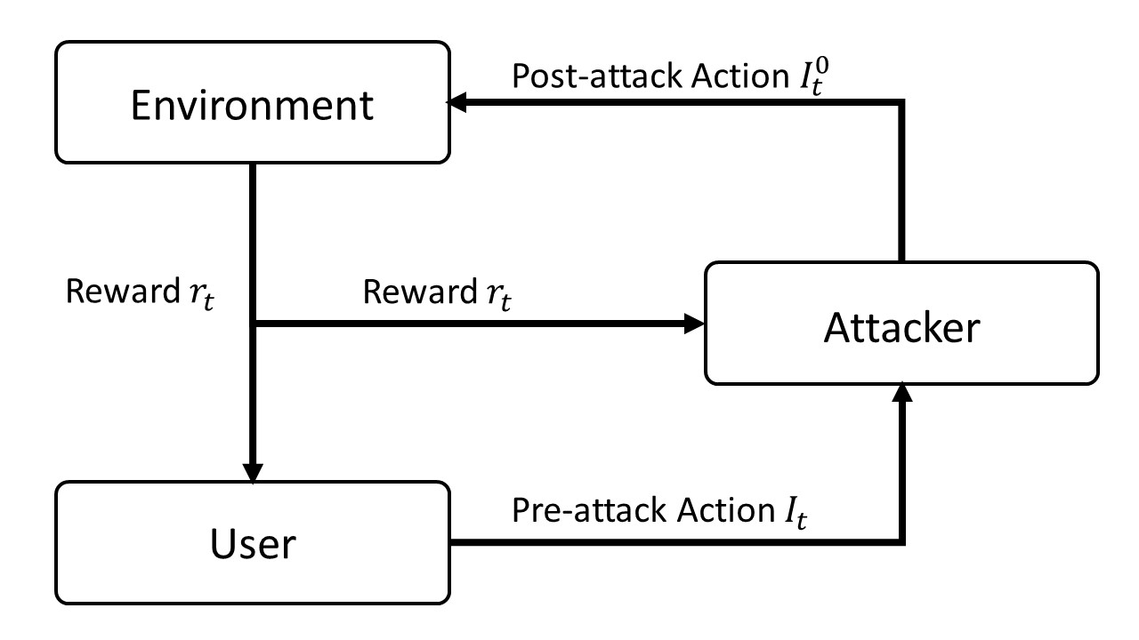
In this paper, we introduce a novel adversary setting, in which the attacker sits between the user and the environment. The attacker can monitor the actions of the user and the reward signals from the environment. Furthermore, the attacker can introduce action-manipulation attacks on stochastic bandits. In particular, at each round t𝑡t, after the user chooses an arm Itsubscript𝐼𝑡I_{t}, the attacker can manipulate the user’s action by changing Itsubscript𝐼𝑡I_{t} to another It0{1,,K}superscriptsubscript𝐼𝑡01𝐾I_{t}^{0}\in\{1,\dots,K\}. If the attacker decides not to attack, It0=Itsuperscriptsubscript𝐼𝑡0subscript𝐼𝑡I_{t}^{0}=I_{t}. The environment generates a random reward rtsubscript𝑟𝑡r_{t} from the reward distribution of post-attack arm It0superscriptsubscript𝐼𝑡0I_{t}^{0}. Then the user and the attacker receive reward rtsubscript𝑟𝑡r_{t} from the environment.

Refer to caption
Figure 1: Action-manipulation attack model

Without loss of generality and for notation convenience, we assume arm K𝐾K is the “attack target” arm or target arm. The attacker’s goal is to manipulate the user into pulling the target arm very frequently but by making attacks as rarely as possible. Define the set of rounds when the attacker decides to attack as 𝒞:={t:tT,It0It}assign𝒞conditional-set𝑡formulae-sequence𝑡𝑇superscriptsubscript𝐼𝑡0subscript𝐼𝑡\mathcal{C}:=\{t:t\leq T,I_{t}^{0}\not=I_{t}\}. The cumulative attack cost is the total number of rounds where the attacker decides to attack, i.e., |𝒞|𝒞|\mathcal{C}|.

In this paper, we assume that the reward distribution of arm i𝑖i follows σ2superscript𝜎2\sigma^{2}-sub-Gaussian distributions with mean μisubscript𝜇𝑖\mu_{i}. Denote the true reward vector as 𝝁=[μ1,,μK]𝝁subscript𝜇1subscript𝜇𝐾\boldsymbol{\mu}=[\mu_{1},\cdots,\mu_{K}]. Neither the user nor the attacker knows 𝝁𝝁\boldsymbol{\mu}, but σ2superscript𝜎2\sigma^{2} is known to both the user and the attacker. Define the difference of mean value of arm i𝑖i and j𝑗j as Δi,j=μiμjsubscriptΔ𝑖𝑗subscript𝜇𝑖subscript𝜇𝑗\Delta_{i,j}=\mu_{i}-\mu_{j}. Furthermore, we refer to the best arm as iO=argmaxiμisubscript𝑖𝑂subscript𝑖subscript𝜇𝑖i_{O}=\arg\max_{i}\mu_{i} and the worst arm as iW=argminiμisubscript𝑖𝑊subscript𝑖subscript𝜇𝑖i_{W}=\arg\min_{i}\mu_{i}.

Note that the assumption that the attacker does not know 𝝁𝝁\boldsymbol{\mu} is important. If the attacker knows these values, the attacker can adopt a trivial oracle attack scheme: whenever the user pulls a non-target arm Itsubscript𝐼𝑡I_{t}, the attacker changes Itsubscript𝐼𝑡I_{t} to the worst arm iWsubscript𝑖𝑊i_{W}. It is easy to show that, if the user uses a bandit algorithm that has a regret upper bounded of 𝒪(log(T))𝒪𝑇\mathcal{O}(\log(T)) when there is no attack, the oracle attack scheme can force the user to pull the target arm T𝒪(log(T))𝑇𝒪𝑇T-\mathcal{O}(\log(T)) times, using a cumulative cost |𝒞|=𝒪(log(T))𝒞𝒪𝑇|\mathcal{C}|=\mathcal{O}(\log(T)). However, the oracle attack scheme is not practical when the true reward vector is unknown. In this paper, we will first design an effective attack scheme, which does not assume the knowledge of true reward vector and nearly matches the performance of the oracle attack scheme, to attack the UCB algorithm. We will then design a new bandit algorithm that is robust against the action-manipulation attack.

The action-manipulation attack considered here is different from reward-manipulation attacks introduced by interesting recent work [22, 23], where the attacker can change the reward signal from the environment. In the setting considered in [22, 23], the attacker can change the reward signal rtsubscript𝑟𝑡r_{t} from the environment to an arbitrary value chosen by the attacker. Correspondingly, the cumulative attack cost in [22, 23] is defined to be the sum of the absolute value of the changes on the reward. Compared with the reward-manipulation attacks discussed above, the action-manipulation attack is more difficult to carry out. In particular, as the action-manipulation attack only changes the action, it can impact but does not have direct control of the reward signal, which will be a random variable drawn from a distribution depending on the action chosen by the attacker. This is in contrast to reward-manipulation attacks where an attacker can change the rewards to any value.

III Attack on UCB and Cost Analysis

In this section, we use UCB algorithm as an example to illustrate the effects of action-manipulation attack. We will introduce LCB attack strategy on the UCB bandit algorithm and analyze the cost.

III-A Attack strategy

UCB algorithm [28] is one of the most popular bandit algorithm. In the UCB algorithm, the user initially pulls each of the K𝐾K arms once in the first K𝐾K rounds. After that, the user chooses arms according to

It=argmaxi{μ^i(t1)+3σlogtNi(t1)}.subscript𝐼𝑡subscript𝑖subscript^𝜇𝑖𝑡13𝜎𝑡subscript𝑁𝑖𝑡1\displaystyle I_{t}=\arg\max_{i}\left\{\hat{\mu}_{i}(t-1)+3\sigma\sqrt{\frac{\log t}{N_{i}(t-1)}}\right\}. (3)

Under the action-manipulation attack, as the user does not know that rtsubscript𝑟𝑡r_{t} is generated from arm It0superscriptsubscript𝐼𝑡0I_{t}^{0} instead of Itsubscript𝐼𝑡I_{t}, the empirical mean μ^i(t)subscript^𝜇𝑖𝑡\hat{\mu}_{i}(t) computed using (1) is not a proper estimate of the true mean reward of arm i𝑖i anymore. On the other hand, the attack is able to obtain a good estimate of μisubscript𝜇𝑖\mu_{i} by

μ^i0(t):=Ni0(t)1sτi0(t)rs,assignsuperscriptsubscript^𝜇𝑖0𝑡superscriptsubscript𝑁𝑖0superscript𝑡1subscript𝑠superscriptsubscript𝜏𝑖0𝑡subscript𝑟𝑠\displaystyle\hat{\mu}_{i}^{0}(t):=N_{i}^{0}(t)^{-1}\sum_{s\in\tau_{i}^{0}(t)}r_{s}, (4)

where τi0(t):={s:st,Is0=i}assignsuperscriptsubscript𝜏𝑖0𝑡conditional-set𝑠formulae-sequence𝑠𝑡superscriptsubscript𝐼𝑠0𝑖\tau_{i}^{0}(t):=\{s:s\leq t,I_{s}^{0}=i\} is the set of rounds up to t𝑡t when the attacker changes an arm to arm i𝑖i, and Ni0(t)=|τi0(t)|superscriptsubscript𝑁𝑖0𝑡superscriptsubscript𝜏𝑖0𝑡N_{i}^{0}(t)=|\tau_{i}^{0}(t)| is the number of pulls of post-attack arm i𝑖i up to round t𝑡t. This information gap provides a chance for attack. In this section, we assume that the target arm is not the worst arm, i.e., μK>μiWsubscript𝜇𝐾subscript𝜇subscript𝑖𝑊\mu_{K}>\mu_{i_{W}}. We will discuss the case where the target arm is the worst arm in Section III-C.

The proposed attack strategy works as follows. In the first K𝐾K rounds, the attacker does not attack. After that, at round t𝑡t, if the user chooses a non-target arm Itsubscript𝐼𝑡I_{t}, the attacker changes it to arm It0superscriptsubscript𝐼𝑡0I_{t}^{0} that has the smallest lower confidence bound (LCB):

It0=argmini{μ^i0(t1)CB(Ni0(t1))},superscriptsubscript𝐼𝑡0subscript𝑖superscriptsubscript^𝜇𝑖0𝑡1CBsuperscriptsubscript𝑁𝑖0𝑡1\displaystyle I_{t}^{0}=\arg\min_{i}\left\{\hat{\mu}_{i}^{0}(t-1)-\textbf{CB}\left(N_{i}^{0}(t-1)\right)\right\}, (5)

where

CB(N)=2σ2Nlogπ2KN23δ.CB𝑁2superscript𝜎2𝑁superscript𝜋2𝐾superscript𝑁23𝛿\textbf{CB}(N)=\sqrt{\frac{2\sigma^{2}}{N}\log\frac{\pi^{2}KN^{2}}{3\delta}}. (6)

Here δ𝛿\delta is a parameter that is related to the probability statements in the analytical results presented in Section III-B. We call our scheme as LCB attack strategy. If at round t𝑡t the user chooses the target arm, the attacker does not attack. Thus the cumulative attack cost of our LCB attack scheme is equal to the total of times when the non-target arms are selected by the user. The algorithm is summarized in Algorithm 1.

0:    
The user’s bandit algorithm, target arm K𝐾K
1:  for t=1,2,𝑡12t=1,2,\dots do
2:     The user chooses arm Itsubscript𝐼𝑡I_{t} to pull according to UCB algorithm (3). 
3:     if It=Ksubscript𝐼𝑡𝐾I_{t}=K then
4:        The attacker does not attack, and It0=Itsuperscriptsubscript𝐼𝑡0subscript𝐼𝑡I_{t}^{0}=I_{t}.
5:     else
6:        The attacker attacks and changes arm Itsubscript𝐼𝑡I_{t} to It0superscriptsubscript𝐼𝑡0I_{t}^{0} chosen according to (5).
7:     end if
8:     The environment generates reward rtsubscript𝑟𝑡r_{t} from arm It0superscriptsubscript𝐼𝑡0I_{t}^{0}.
9:     The attacker and the user receive rtsubscript𝑟𝑡r_{t}.
10:  end for
Algorithm 1 LCB attack strategy on UCB algorithm

Here, we highlight the main idea why LCB attack strategy works. As discussed in Section II, if the attacker knows which arm is the worst, the attacker can simply change the action to the worst arm when the user pulls the non-target arm. The main idea of the attack scheme is to estimate the mean of each arm, and change the non-target arm to the arm whose lower confidence bound is the smallest. Effectively, this will almost always change the non-target arm to the worst arm. More formally, for iK𝑖𝐾i\neq K, we will show that this attack strategy will ensure that μ^isubscript^𝜇𝑖\hat{\mu}_{i} computed using (1) by the user converges to μiWsubscript𝜇subscript𝑖𝑊\mu_{i_{W}}. On the other hand, as the attacker does not attack when the user selects K𝐾K, μ^Ksubscript^𝜇𝐾\hat{\mu}_{K} computed by the user will still converge to the true mean μKsubscript𝜇𝐾\mu_{K} with NKsubscript𝑁𝐾N_{K} increasing. Because the assumption that the target arm is not the worst, which implies that μK>μiWsubscript𝜇𝐾subscript𝜇subscript𝑖𝑊\mu_{K}>\mu_{i_{W}}, μ^isubscript^𝜇𝑖\hat{\mu}_{i} could be smaller than μ^Ksubscript^𝜇𝐾\hat{\mu}_{K}. Then the user will rarely pull the non-target arms as μ^isubscript^𝜇𝑖\hat{\mu}_{i} is smaller than μ^Ksubscript^𝜇𝐾\hat{\mu}_{K}. Hence, the attack cost would also be small. The rigorous analysis of the cost will be provided in Section III-B.

III-B Cost analysis

To analyze the cost of the proposed scheme, we need to track μ^i0(t)superscriptsubscript^𝜇𝑖0𝑡\hat{\mu}_{i}^{0}(t), the estimate obtained by the attacker using (4), and μ^i(t)subscript^𝜇𝑖𝑡\hat{\mu}_{i}(t), the estimate obtained by the user using (1).

The analysis of μ^i0(t)superscriptsubscript^𝜇𝑖0𝑡\hat{\mu}_{i}^{0}(t) is relatively simple, as the attacker knows which arm is truly pulled and hence μ^i0(t)superscriptsubscript^𝜇𝑖0𝑡\hat{\mu}_{i}^{0}(t) is the true estimate of the mean of arm i𝑖i. Define event

1:={i,t>K:|μ^i0(t)μi|<CB(Ni0(t))}.assignsubscript1conditional-setfor-all𝑖for-all𝑡𝐾superscriptsubscript^𝜇𝑖0𝑡subscript𝜇𝑖CBsuperscriptsubscript𝑁𝑖0𝑡\displaystyle\mathcal{E}_{1}:=\{\forall i,\forall t>K:|\hat{\mu}_{i}^{0}(t)-\mu_{i}|<\textbf{CB}(N_{i}^{0}(t))\}. (7)

Roughly speaking, event 1subscript1\mathcal{E}_{1} is the event that the empirical mean computed by the attacker using (4) is close to the true mean. The following lemma, proved in [22], shows that the attacker can accurately estimate the average reward to each arm.

Lemma 1.

(Lemma 1 in [22]) For δ(0,1)𝛿01\delta\in(0,1), (1)>1δsubscript11𝛿\mathbb{P}(\mathcal{E}_{1})>1-\delta.

The analysis of μ^i(t)subscript^𝜇𝑖𝑡\hat{\mu}_{i}(t) computed by the user is more complicated. When the user pulls arm i𝑖i, because of the action-manipulation attacks, the random rewards may be drawn from different reward distributions. Define τi,j(t):={s:st,Is=iandIs0=j}assignsubscript𝜏𝑖𝑗𝑡conditional-set𝑠formulae-sequence𝑠𝑡subscript𝐼𝑠𝑖andsuperscriptsubscript𝐼𝑠0𝑗\tau_{i,j}(t):=\{s:s\leq t,I_{s}=i\ \text{and}\ I_{s}^{0}=j\} as the set of rounds up to t𝑡t when the user chooses arm i𝑖i and the attacker changes it to arm j𝑗j. Lemma 2 shows a high-probability confidence bounds of μ^i,j(t):=Ni,j(t)1sτi,j(t)rsassignsubscript^𝜇𝑖𝑗𝑡subscript𝑁𝑖𝑗superscript𝑡1subscript𝑠subscript𝜏𝑖𝑗𝑡subscript𝑟𝑠\hat{\mu}_{i,j}(t):=N_{i,j}(t)^{-1}\sum_{s\in\tau_{i,j}(t)}r_{s}, the empirical mean rewards of a part of arm i𝑖i whose post-attack arm is j𝑗j, where Ni,j(t):=|τi,j(t)|assignsubscript𝑁𝑖𝑗𝑡subscript𝜏𝑖𝑗𝑡N_{i,j}(t):=|\tau_{i,j}(t)|. Define event

2:={i,j,t>K:|μ^i,j(t)μj|<2σ2Ni,j(t)logπ2K2(Ni,j(t))23δ}.assignsubscript2conditional-setfor-all𝑖for-all𝑗for-all𝑡𝐾subscript^𝜇𝑖𝑗𝑡subscript𝜇𝑗2superscript𝜎2subscript𝑁𝑖𝑗𝑡superscript𝜋2superscript𝐾2superscriptsubscript𝑁𝑖𝑗𝑡23𝛿\begin{split}\mathcal{E}_{2}:=\left\{\forall i,\forall j,\forall t>K:|\hat{\mu}_{i,j}(t)-\mu_{j}|<\right.&\\ \left.\sqrt{\frac{2\sigma^{2}}{N_{i,j}(t)}\log\frac{\pi^{2}K^{2}(N_{i,j}(t))^{2}}{3\delta}}\right\}&.\end{split} (8)
Lemma 2.

For δ(0,1)𝛿01\delta\in(0,1), (2)>1δsubscript21𝛿\mathbb{P}(\mathcal{E}_{2})>1-\delta.

Proof.

Please refer to Appendix A. ∎

Although rssubscript𝑟𝑠r_{s} in (1), used to calculate μ^i(t)subscript^𝜇𝑖𝑡\hat{\mu}_{i}(t), may be drawn from different reward distributions, we can build a high-probability bound of μ^i(t)subscript^𝜇𝑖𝑡\hat{\mu}_{i}(t) with the help of Lemma 2.

Lemma 3.

Under event 2subscript2\mathcal{E}_{2}, for all arm i𝑖i and all t>K𝑡𝐾t>K, we have

|μ^i(t)1Ni(t)sτi(t)μIs0|<β(Ni(t)),subscript^𝜇𝑖𝑡1subscript𝑁𝑖𝑡subscript𝑠subscript𝜏𝑖𝑡subscript𝜇superscriptsubscript𝐼𝑠0𝛽subscript𝑁𝑖𝑡\displaystyle\left|\hat{\mu}_{i}(t)-\frac{1}{N_{i}(t)}\sum_{s\in\tau_{i}(t)}\mu_{I_{s}^{0}}\right|<\beta(N_{i}(t)), (9)

where

β(Ni(t))=2σ2KNi(t)logπ2(Ni(t))23δ.𝛽subscript𝑁𝑖𝑡2superscript𝜎2𝐾subscript𝑁𝑖𝑡superscript𝜋2superscriptsubscript𝑁𝑖𝑡23𝛿\displaystyle\beta(N_{i}(t))=\sqrt{\frac{2\sigma^{2}K}{N_{i}(t)}\log\frac{\pi^{2}(N_{i}(t))^{2}}{3\delta}}. (10)
Proof.

Please refer to Appendix B. ∎

Under events 1subscript1\mathcal{E}_{1} and 2subscript2\mathcal{E}_{2}, we can build a connection between u^i(t)subscript^𝑢𝑖𝑡\hat{u}_{i}(t) and μiWsubscript𝜇subscript𝑖𝑊\mu_{i_{W}}. In the proposed LCB attack strategy, the attacker explores and exploits the worst arm by a lower confidence bound method. Thus, when the user pulls a non-target arm, the attacker changes it to the worst arm at most of rounds, which means that for all iK𝑖𝐾i\neq K, u^i(t)subscript^𝑢𝑖𝑡\hat{u}_{i}(t) will converge to μiWsubscript𝜇subscript𝑖𝑊\mu_{i_{W}} as Ni(t)subscript𝑁𝑖𝑡N_{i}(t) increases. Lemma 4 shows the relationship between u^i(t)subscript^𝑢𝑖𝑡\hat{u}_{i}(t) and μiWsubscript𝜇subscript𝑖𝑊\mu_{i_{W}}.

Lemma 4.

Under events 1subscript1\mathcal{E}_{1} and 2subscript2\mathcal{E}_{2}, using LCB attack strategy 1, we have

μ^i(t)uiWsubscript^𝜇𝑖𝑡subscript𝑢subscript𝑖𝑊\displaystyle\hat{\mu}_{i}(t)\leq u_{i_{W}} +1Ni(t)jiW8σ2Δj,iWlogπ2Kt23δ1subscript𝑁𝑖𝑡subscript𝑗subscript𝑖𝑊8superscript𝜎2subscriptΔ𝑗subscript𝑖𝑊superscript𝜋2𝐾superscript𝑡23𝛿\displaystyle+\frac{1}{N_{i}(t)}\sum_{j\neq i_{W}}\frac{8\sigma^{2}}{\Delta_{j,i_{W}}}\log\frac{\pi^{2}Kt^{2}}{3\delta} (11)
+2σ2KNi(t)logπ2(Ni(t))23δ,i,t.2superscript𝜎2𝐾subscript𝑁𝑖𝑡superscript𝜋2superscriptsubscript𝑁𝑖𝑡23𝛿for-all𝑖𝑡\displaystyle+\sqrt{\frac{2\sigma^{2}K}{N_{i}(t)}\log\frac{\pi^{2}(N_{i}(t))^{2}}{3\delta}},\forall i,t. (12)
Proof.

Please refer to Appendix C. ∎

Lemma 4 shows an upper bound of the empirical mean reward of pre-attack arm i𝑖i, for all arm iK𝑖𝐾i\neq K. Our main results is the following upper bound on the attack cost |𝒞|𝒞|\mathcal{C}|.

Theorem 1.

With probability at least 12δ12𝛿1-2\delta, when T(π2K3δ)25𝑇superscriptsuperscript𝜋2𝐾3𝛿25T\geq\left(\frac{\pi^{2}K}{3\delta}\right)^{\frac{2}{5}}, using LCB attack strategy specified in Algorithm 1, the attacker can manipulate the user into pulling the target arm in at least T|𝒞|𝑇𝒞T-|\mathcal{C}| rounds, with an attack cost

|𝒞|K14ΔK,iW2(3σlogT+2σ2Klogπ2T23δ+((3σlogT+2σ2Klogπ2T23δ)2+4ΔK,iWjiW8σ2Δj,iWlogπ2KT23δ)12)2.𝒞𝐾14superscriptsubscriptΔ𝐾subscript𝑖𝑊2superscript3𝜎𝑇2superscript𝜎2𝐾superscript𝜋2superscript𝑇23𝛿superscriptsuperscript3𝜎𝑇2superscript𝜎2𝐾superscript𝜋2superscript𝑇23𝛿24subscriptΔ𝐾subscript𝑖𝑊subscript𝑗subscript𝑖𝑊8superscript𝜎2subscriptΔ𝑗subscript𝑖𝑊superscript𝜋2𝐾superscript𝑇23𝛿122\begin{split}|\mathcal{C}|\leq&\frac{K-1}{4\Delta_{K,i_{W}}^{2}}\left(3\sigma\sqrt{\log T}+\sqrt{2\sigma^{2}K\log\frac{\pi^{2}T^{2}}{3\delta}}\right.\\ &+\left(\left(3\sigma\sqrt{\log T}+\sqrt{2\sigma^{2}K\log\frac{\pi^{2}T^{2}}{3\delta}}\right)^{2}\right.\\ &\left.\left.+4\Delta_{K,i_{W}}\sum_{j\neq i_{W}}\frac{8\sigma^{2}}{\Delta_{j,i_{W}}}\log\frac{\pi^{2}KT^{2}}{3\delta}\right)^{\frac{1}{2}}\right)^{2}.\end{split} (13)
Proof.

Please refer to Appendix D. ∎

The expression of the cost bound in Theorem 1 is complicated. The following corollary provides a simpler bound that is more explicit and interpretable.

Corollary 1.

Under the same assumptions in Theorem 1, the total attack cost |𝒞|𝒞|\mathcal{C}| of Algorithm 1 is upper bounded by

𝒪(Kσ2logTΔK,iW2(K+jiWΔK,iWΔj,iW+KjiWΔK,iWΔj,iW)),𝒪𝐾superscript𝜎2𝑇superscriptsubscriptΔ𝐾subscript𝑖𝑊2𝐾subscript𝑗subscript𝑖𝑊subscriptΔ𝐾subscript𝑖𝑊subscriptΔ𝑗subscript𝑖𝑊𝐾subscript𝑗subscript𝑖𝑊subscriptΔ𝐾subscript𝑖𝑊subscriptΔ𝑗subscript𝑖𝑊\begin{split}\mathcal{O}\left(\frac{K\sigma^{2}\log T}{\Delta_{K,i_{W}}^{2}}\left(K+\sum_{j\neq i_{W}}\frac{\Delta_{K,i_{W}}}{\Delta_{j,i_{W}}}+\sqrt{K\sum_{j\neq i_{W}}\frac{\Delta_{K,i_{W}}}{\Delta_{j,i_{W}}}}\right)\right),\end{split} (14)

and the total number of target arm pulls is T|𝒞|𝑇𝒞T-|\mathcal{C}|.

From Corollary 1, we can see that the attack cost scales as logT𝑇\log T. Two important constants σΔK,iW𝜎subscriptΔ𝐾subscript𝑖𝑊\frac{\sigma}{\Delta_{K,i_{W}}} and jiWΔK,iWΔj,iWsubscript𝑗subscript𝑖𝑊subscriptΔ𝐾subscript𝑖𝑊subscriptΔ𝑗subscript𝑖𝑊\sum_{j\neq i_{W}}\frac{\Delta_{K,i_{W}}}{\Delta_{j,i_{W}}} have impact on the prelog factor. In Section V, we provide some numerical examples to illustrate the effects of these two constants on the attack cost.

III-C Attacks fail when the target arm is the worst arm

One weakness of our LCB attack strategy is that the attack target arm is necessarily a non-worst arm. In the LCB attack strategy, the attacker can not force the user to pull the worst arm very frequently by spending only logarithmic cost. The main reason is that, when the target arm is the worst, the average reward of each arm is larger or equal to that of the target arm. As the result, our attack scheme is not able to ensure that the target arm has a higher expected reward than the user’s estimate of the rewards of other arms. In fact, the following theorem shows that all action-manipulation attack can not manipulate the UCB algorithm into pulling the worst arm more than T𝒪(log(T))𝑇𝒪𝑇T-\mathcal{O}(\log(T)) by spending only logarithmic cost.

Theorem 2.

Let δ<12𝛿12\delta<\frac{1}{2}. Suppose the attack cost is limited by 𝒪(log(T))𝒪𝑇\mathcal{O}(\log(T)), there is no attack that can force the UCB algorithm to pick the worst arm more than T𝒪(Tα)𝑇𝒪superscript𝑇𝛼T-\mathcal{O}(T^{\alpha}) times with probability at least 1δ1𝛿1-\delta, in which α<964K𝛼964𝐾\alpha<\frac{9}{64K}.

Proof.

Please refer to Appendix E. ∎

This theorem shows a contrast between the case where the target arm is not the worst arm and the case where the target arm is the worst arm. If the target arm is not the worst arm, our scheme is able to force the user to pick the target arm T𝒪(log(T))𝑇𝒪𝑇T-\mathcal{O}(\log(T)) times with only logarithmic cost. On the other hand, if the target arm is the worst, Theorem 2 shows that there is no attack strategy that can force the user to pick the worst arm more than T𝒪(Tα)𝑇𝒪superscript𝑇𝛼T-\mathcal{O}(T^{\alpha}) times while incurring only logarithmic cost.

IV Robust algorithm and regret analysis

The results in Section III exposes a significant security threat of the action-manipulation attacks on MABs. Under only 𝒪(log(T))𝒪𝑇\mathcal{O}(\log(T)) times of attacks carried out using the proposed LCB strategy, the UCB algorithm will almost always pull the target arm selected by the attacker. Although there are some defense algorithms [24] and universal best arm identification schemes [29] for stochastic or adversarial bandit, they do not apply to action-manipulation attack setting. This motivates us to design a new bandit algorithm that is robust against action-manipulation attacks. In this section, we propose such a robust bandit algorithm and analyze its regret.

IV-A Robust Bandit algorithm

In this section, we assume that a valid upper bound A𝐴A for the cumulative attack cost |𝒞|𝒞|\mathcal{C}| is known for the user, although the user do not have to know the exact cumulative attack cost |𝒞|𝒞|\mathcal{C}|. A𝐴A does not need to be constant, it can scale with T𝑇T. In other words, for a given A𝐴A, our proposed algorithm is robust to all action-manipulation attacks with a cumulative attack cost |𝒞|<A𝒞𝐴|\mathcal{C}|<A. This assumption is reasonable, as if the cost is unbounded, it will not be possible to design a robust scheme.

We first introduce some notation. Denote 𝐍(t1):=(N1(t1),,NK(t1))assign𝐍𝑡1subscript𝑁1𝑡1subscript𝑁𝐾𝑡1\mathbf{N}(t-1):=(N_{1}(t-1),\dots,N_{K}(t-1)) as the vector counting how many times each action has been taken by the user, and 𝝁^(t1)=(μ^1(t1),,μ^K(t1))bold-^𝝁𝑡1subscript^𝜇1𝑡1subscript^𝜇𝐾𝑡1\boldsymbol{\hat{\mu}}(t-1)=(\hat{\mu}_{1}(t-1),\dots,\hat{\mu}_{K}(t-1)) as the vector of the sample means computed by the user. The proposed algorithm is a modified UCB method by taking the maximum possible mean estimate offset due to attack into consideration. We name our scheme as maximum offset UCB (MOUCB).

The proposed MOUCB works as follows. In the first 2AK2𝐴𝐾2AK rounds, MOUCB algorithm pulls each arm 2A2𝐴2A times. After that, at round t𝑡t, the user chooses an arm Itsubscript𝐼𝑡I_{t} by a modified UCB method:

It=argmaxa{μ^a(t1)+β(Na(t1))+γ(𝝁^(t1),𝐍(t1))},subscript𝐼𝑡subscript𝑎subscript^𝜇𝑎𝑡1𝛽subscript𝑁𝑎𝑡1𝛾bold-^𝝁𝑡1𝐍𝑡1\begin{split}I_{t}=\arg\max_{a}&\left\{\hat{\mu}_{a}(t-1)+\beta(N_{a}(t-1))\right.\\ &\left.\hskip 14.22636pt+\gamma(\boldsymbol{\hat{\mu}}(t-1),\mathbf{N}(t-1))\right\},\end{split} (15)

where

γ(𝝁^(t1),𝐍(t1))=2ANa(t1)𝛾bold-^𝝁𝑡1𝐍𝑡12𝐴subscript𝑁𝑎𝑡1\displaystyle\gamma(\boldsymbol{\hat{\mu}}(t-1),\mathbf{N}(t-1))=\frac{2A}{N_{a}(t-1)}
maxi,j{μ^i(t1)μ^j(t1)+β(Ni(t1))+β(Nj(t1))},subscript𝑖𝑗subscript^𝜇𝑖𝑡1subscript^𝜇𝑗𝑡1𝛽subscript𝑁𝑖𝑡1𝛽subscript𝑁𝑗𝑡1\displaystyle\max_{i,j}\left\{\hat{\mu}_{i}(t-1)-\hat{\mu}_{j}(t-1)+\beta(N_{i}(t-1))+\beta(N_{j}(t-1))\right\},

and

β(N)=2σ2KNlogπ2N23δ.𝛽𝑁2superscript𝜎2𝐾𝑁superscript𝜋2superscript𝑁23𝛿\begin{split}\beta(N)=\sqrt{\frac{2\sigma^{2}K}{N}\log\frac{\pi^{2}N^{2}}{3\delta}}.\end{split} (16)

The algorithm is summarized in Algorithm 2.

0:    
A valid upper bound A𝐴A for the cumulative attack cost.
1:  for t=1,2,𝑡12t=1,2,\dots do
2:     if t2AK𝑡2𝐴𝐾t\leq 2AK then
3:        The user pulls the arm whose pull count is the smallest, i.e. It=argminiNi(t1)subscript𝐼𝑡subscript𝑖subscript𝑁𝑖𝑡1I_{t}=\arg\min_{i}N_{i}(t-1)
4:     else
5:        The user chooses arm Itsubscript𝐼𝑡I_{t} to pull according (15).
6:     end if
7:     if The attacker decides to attack then
8:        The attacker attacks and changes Itsubscript𝐼𝑡I_{t} to It0superscriptsubscript𝐼𝑡0I_{t}^{0}.
9:     else
10:        The attacker does not attack and It0=Itsuperscriptsubscript𝐼𝑡0subscript𝐼𝑡I_{t}^{0}=I_{t}.
11:     end if
12:     The environment generates reward rtsubscript𝑟𝑡r_{t} from arm It0superscriptsubscript𝐼𝑡0I_{t}^{0}.
13:     The attacker and the user receive rtsubscript𝑟𝑡r_{t}.
14:  end for
Algorithm 2 Proposed MOUCB bandit algorithm

Compared with the original UCB algorithm in (3), the main difference is the additional term γ(𝝁^(t1),𝐍(t1))𝛾bold-^𝝁𝑡1𝐍𝑡1\gamma(\boldsymbol{\hat{\mu}}(t-1),\mathbf{N}(t-1)) in (15). We now highlight the main idea why our bandit algorithm works and the role of this additional term. In particular, in the standard multi-armed stochastic bandit problem, μ^i(t)subscript^𝜇𝑖𝑡\hat{\mu}_{i}(t) is a proper estimation of μisubscript𝜇𝑖\mu_{i}, the true mean reward of arm i𝑖i. However, under the action-manipulation attacks, as the user does not know which arm is used to generate rtsubscript𝑟𝑡r_{t}, μ^i(t)subscript^𝜇𝑖𝑡\hat{\mu}_{i}(t) is not a proper estimate of the true mean reward anymore. However, we can try to find a good bound of the true mean reward. If we know ΔiO,iWsubscriptΔsubscript𝑖𝑂subscript𝑖𝑊\Delta_{i_{O},i_{W}}, the reward difference between the optimal arm and the worst arm, we can describe the maximum offset of the mean rewards caused by the attack. In particular, we have

μiANi(t)ΔiO,iW1Ni(t)sτi(t)μIs0μi+ANi(t)ΔiO,iW,subscript𝜇𝑖𝐴subscript𝑁𝑖𝑡subscriptΔsubscript𝑖𝑂subscript𝑖𝑊1subscript𝑁𝑖𝑡subscript𝑠subscript𝜏𝑖𝑡subscript𝜇superscriptsubscript𝐼𝑠0subscript𝜇𝑖𝐴subscript𝑁𝑖𝑡subscriptΔsubscript𝑖𝑂subscript𝑖𝑊\mu_{i}-\frac{A}{N_{i}(t)}\Delta_{i_{O},i_{W}}\leq\frac{1}{N_{i}(t)}\sum_{s\in\tau_{i}(t)}\mu_{I_{s}^{0}}\leq\mu_{i}+\frac{A}{N_{i}(t)}\Delta_{i_{O},i_{W}}, (17)

which implies

μiANi(t)ΔiO,iW+1Ni(t)sτi(t)μIs0.subscript𝜇𝑖𝐴subscript𝑁𝑖𝑡subscriptΔsubscript𝑖𝑂subscript𝑖𝑊1subscript𝑁𝑖𝑡subscript𝑠subscript𝜏𝑖𝑡subscript𝜇superscriptsubscript𝐼𝑠0\mu_{i}\leq\frac{A}{N_{i}(t)}\Delta_{i_{O},i_{W}}+\frac{1}{N_{i}(t)}\sum_{s\in\tau_{i}(t)}\mu_{I_{s}^{0}}. (18)

In (18), the first term in the right hand side is the maximum offset that an attacker can introduce regardless of the attack strategy. The second term in the right hand side is related to the mean estimated by the user. In particular, under event 2subscript2\mathcal{E}_{2}, as shown in Lemma 3, we have

1Ni(t)sτi(t)μIs0<μ^i(t)+β(Ni(t)).1subscript𝑁𝑖𝑡subscript𝑠subscript𝜏𝑖𝑡subscript𝜇superscriptsubscript𝐼𝑠0subscript^𝜇𝑖𝑡𝛽subscript𝑁𝑖𝑡\displaystyle\frac{1}{N_{i}(t)}\sum_{s\in\tau_{i}(t)}\mu_{I_{s}^{0}}<\hat{\mu}_{i}(t)+\beta(N_{i}(t)). (19)

Hence, regardless the attack strategy, we have a upper confidence bound on μisubscript𝜇𝑖\mu_{i}:

μiμ^i(t)+ANi(t)ΔiO,iW+β(Ni(t)).subscript𝜇𝑖subscript^𝜇𝑖𝑡𝐴subscript𝑁𝑖𝑡subscriptΔsubscript𝑖𝑂subscript𝑖𝑊𝛽subscript𝑁𝑖𝑡\mu_{i}\leq\hat{\mu}_{i}(t)+\frac{A}{N_{i}(t)}\Delta_{i_{O},i_{W}}+\beta(N_{i}(t)). (20)

In our case, however, ΔiO,iWsubscriptΔsubscript𝑖𝑂subscript𝑖𝑊\Delta_{i_{O},i_{W}} is also unknown. In our algorithm, we obtain a high-probability bound on ΔiO,iWsubscriptΔsubscript𝑖𝑂subscript𝑖𝑊\Delta_{i_{O},i_{W}}:

ΔiO,iW2maxi,j{μ^iμ^j+β(Ni(t))+β(Nj(t))},subscriptΔsubscript𝑖𝑂subscript𝑖𝑊2subscript𝑖𝑗subscript^𝜇𝑖subscript^𝜇𝑗𝛽subscript𝑁𝑖𝑡𝛽subscript𝑁𝑗𝑡\displaystyle\Delta_{i_{O},i_{W}}\leq 2\max_{i,j}\left\{\hat{\mu}_{i}-\hat{\mu}_{j}+\beta\left(N_{i}(t)\right)+\beta\left(N_{j}(t)\right)\right\}, (21)

which will proved in Lemma 5 below. Now, the second term of (20) becomes γ(𝝁^(t1),𝐍(t1))𝛾bold-^𝝁𝑡1𝐍𝑡1\gamma(\boldsymbol{\hat{\mu}}(t-1),\mathbf{N}(t-1)) if we replace ΔiO,iWsubscriptΔsubscript𝑖𝑂subscript𝑖𝑊\Delta_{i_{O},i_{W}} with the bound (21), and we obtain our final algorithm.

IV-B Regret analysis

Lemma 5 shows a boundary of ΔiO,iWsubscriptΔsubscript𝑖𝑂subscript𝑖𝑊\Delta_{i_{O},i_{W}} the maximum reward difference between any two arms, under event 2subscript2\mathcal{E}_{2}.

Lemma 5.

For δ13𝛿13\delta\leq\frac{1}{3}, t>2AK𝑡2𝐴𝐾t>2AK and under event 2subscript2\mathcal{E}_{2}, MOUCB algorithm have

ΔiO,iW2maxi,j{μ^iμ^j+β(Ni(t))+β(Nj(t))}2ΔiO,iW+8σ2KAlog4π2A23δ.subscriptΔsubscript𝑖𝑂subscript𝑖𝑊2subscript𝑖𝑗subscript^𝜇𝑖subscript^𝜇𝑗𝛽subscript𝑁𝑖𝑡𝛽subscript𝑁𝑗𝑡2subscriptΔsubscript𝑖𝑂subscript𝑖𝑊8superscript𝜎2𝐾𝐴4superscript𝜋2superscript𝐴23𝛿\begin{split}\Delta_{i_{O},i_{W}}&\leq 2\max_{i,j}\left\{\hat{\mu}_{i}-\hat{\mu}_{j}+\beta\left(N_{i}(t)\right)+\beta\left(N_{j}(t)\right)\right\}\\ &\leq 2\Delta_{i_{O},i_{W}}+8\sqrt{\frac{\sigma^{2}K}{A}\log\frac{4\pi^{2}A^{2}}{3\delta}}.\end{split} (22)
Proof.

Please refer to Appendix F. ∎

Using Lemma 5, we now bound the regret of Algorithm 2.

Theorem 3.

Let A𝐴A be an upper bound on the total attack cost |𝒞|𝒞|\mathcal{C}|. For δ13𝛿13\delta\leq\frac{1}{3} and T2AK𝑇2𝐴𝐾T\geq 2AK, MOUCB algorithm has pseudo-regret R¯(T)¯𝑅𝑇\bar{R}(T)

R¯(T)aiOmax{8σ2KΔiO,alogπ2T23δ,A(ΔiO,a+2ΔiO,iW+8σ2KAlog4π2A23δ)},¯𝑅𝑇subscript𝑎subscript𝑖𝑂8superscript𝜎2𝐾subscriptΔsubscript𝑖𝑂𝑎superscript𝜋2superscript𝑇23𝛿𝐴subscriptΔsubscript𝑖𝑂𝑎2subscriptΔsubscript𝑖𝑂subscript𝑖𝑊8superscript𝜎2𝐾𝐴4superscript𝜋2superscript𝐴23𝛿\begin{split}\bar{R}(T)\leq\sum_{a\not=i_{O}}\max&\left\{\frac{8\sigma^{2}K}{\Delta_{i_{O},a}}\log\frac{\pi^{2}T^{2}}{3\delta},A\left(\Delta_{i_{O},a}\right.\right.\\ &\left.\left.+2\Delta_{i_{O},i_{W}}+8\sqrt{\frac{\sigma^{2}K}{A}\log\frac{4\pi^{2}A^{2}}{3\delta}}\right)\right\},\end{split} (23)

with probability at least 1δ1𝛿1-\delta.

Proof.

Please refer to Appendix G. ∎

Theorem 3 reveals that our bandit algorithm is robust to the action-manipulation attacks. If the total attack cost is bounded by 𝒪(logT)𝒪𝑇\mathcal{O}(\log T), the pseudo-regret of MOUCB bandit algorithm is still bounded by 𝒪(logT)𝒪𝑇\mathcal{O}(\log T). This is in contrast with UCB, for which we have shown that the pseudo-regret is 𝒪(T)𝒪𝑇\mathcal{O}(T) with attack cost 𝒪(logT)𝒪𝑇\mathcal{O}(\log T) in Section III. If the total attack cost is up to Ω(logT)Ω𝑇\Omega(\log T), the pseudo-regret of MOUCB bandit algorithm is bounded by 𝒪(A)𝒪𝐴\mathcal{O}(A), which is linear in A𝐴A.

V Numerical results

In this section, we provide numerical examples to illustrate the analytical results obtained. In our simulation, the bandit has 10 arms. The rewards distribution of arm i𝑖i is 𝒩(μi,σ)𝒩subscript𝜇𝑖𝜎\mathcal{N}(\mu_{i},\sigma). The attacker’s target arm is K𝐾K. We let δ=0.05𝛿0.05\delta=0.05. We then run the experiment for multiple trials and in each trial we run T=107𝑇superscript107T=10^{7} rounds.

V-A LCB attack strategy

We first illustrate the impact of the proposed LCB attack strategy on UCB algorithm.
Refer to caption
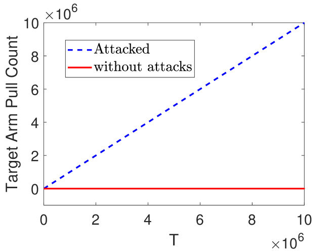
Figure 2: Number of rounds the target arm was pulled

In Figure 2, we fix σ=0.1𝜎0.1\sigma=0.1 and ΔK,iW=0.1subscriptΔ𝐾subscript𝑖𝑊0.1\Delta_{K,i_{W}}=0.1 and compare the number of rounds at which the target arm is pulled with and without attack. In this experiment, the mean rewards of all arms are 1.0, 0.9, 0.8, 0.7, 0.6, 0.5, 0.4, 0.3, 0.1, and 0.2 respectively. Arm K𝐾K is not the worst arm, but its average reward is lower than most arms. The results are averaged over 20 trials. The attacker successfully manipulates the user into pulling the target arm very frequently.
Refer to caption
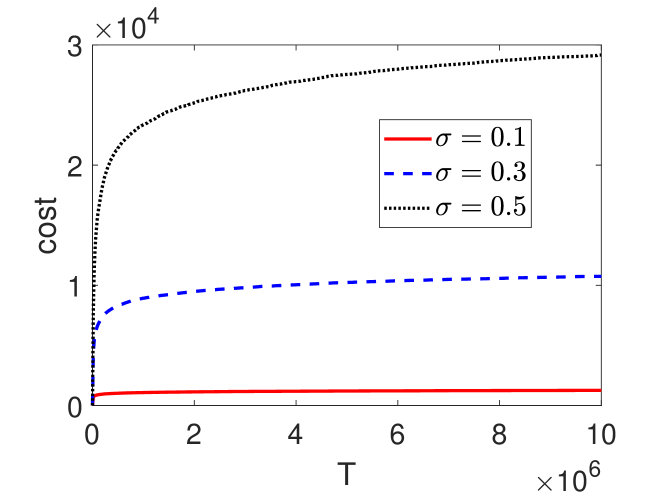
Figure 3: Attack cost vs σΔK,iW𝜎subscriptΔ𝐾subscript𝑖𝑊\frac{\sigma}{\Delta_{K,i_{W}}}

In Figure 3, in order to study how σΔK,iW𝜎subscriptΔ𝐾subscript𝑖𝑊\frac{\sigma}{\Delta_{K,i_{W}}} affects the attack cost, we fix ΔK,iW=0.1subscriptΔ𝐾subscript𝑖𝑊0.1\Delta_{K,i_{W}}=0.1 and set σ𝜎\sigma as 0.1, 0.3 and 0.5 respectively. The mean rewards of all arms are same as above. From the figure, we can see that as σΔK,iW𝜎subscriptΔ𝐾subscript𝑖𝑊\frac{\sigma}{\Delta_{K,i_{W}}} increases, the attack cost increases. In addition, as predicted in our analysis, the attack cost increases with T𝑇T, the total number of rounds, in a logarithmic order.
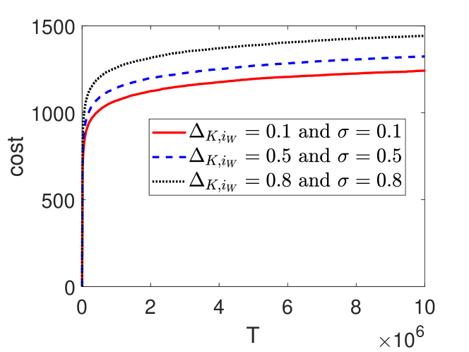
Refer to caption
Figure 4: Attack cost vs jiWΔK,iWΔj,iWsubscript𝑗subscript𝑖𝑊subscriptΔ𝐾subscript𝑖𝑊subscriptΔ𝑗subscript𝑖𝑊\sum_{j\neq i_{W}}\frac{\Delta_{K,i_{W}}}{\Delta_{j,i_{W}}}

Figure 4 illustrates how jiWΔK,iWΔj,iWsubscript𝑗subscript𝑖𝑊subscriptΔ𝐾subscript𝑖𝑊subscriptΔ𝑗subscript𝑖𝑊\sum_{j\neq i_{W}}\frac{\Delta_{K,i_{W}}}{\Delta_{j,i_{W}}} affects the attack cost. In this experiment, we fix σΔK,iW=1𝜎subscriptΔ𝐾subscript𝑖𝑊1\frac{\sigma}{\Delta_{K,i_{W}}}=1 and set ΔK,iWsubscriptΔ𝐾subscript𝑖𝑊\Delta_{K,i_{W}} as 0.2, 0.6 and 0.9 respectively. The mean rewards of all arms are the same as above. The figure illustrates that, as jiWΔK,iWΔj,iWsubscript𝑗subscript𝑖𝑊subscriptΔ𝐾subscript𝑖𝑊subscriptΔ𝑗subscript𝑖𝑊\sum_{j\neq i_{W}}\frac{\Delta_{K,i_{W}}}{\Delta_{j,i_{W}}} increases, the attack cost also increases. This is consistent with our analysis in Corollary 1.

V-B MOUCB bandit algorithm

We now illustrate the effectiveness of MOUCB bandit algorithm.

In this experiment, we use the similar setting as in the simulation of the LCB attack scheme. The mean rewards of all arms are set to be 1.0, 0.8, 0.9, 0.5, 0.2, 0.3, 0.1, 0.4, 0.7, and 0.6 respectively. The total attack cost |𝒞|𝒞|\mathcal{C}| is limited by 2000. A given valid upper bound for total attack cost is A=3000𝐴3000A=3000. The results are averaged over 20 trials.
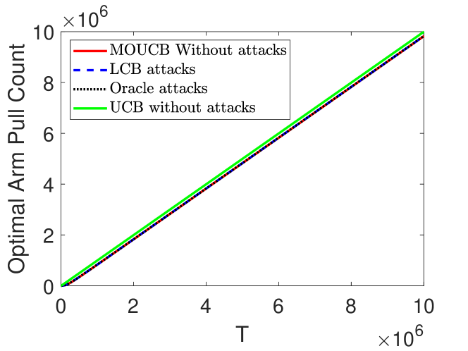
Refer to caption
Figure 5: Comparison of number of rounds the optimal arm was pulled

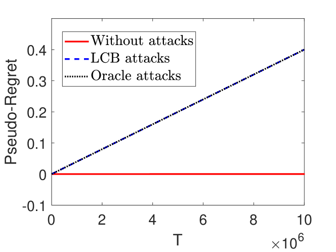
In Figure 5, we simulate MOUCB algorithm with two different attacks, and compare the numbers of rounds when the optimal arm is pulled under these attacks. The first attack is the LCB attack discussed in Section III. The second attack is the oracle attack, in which the attacker knows the true mean reward of arms and implements the oracle attacks that change any non-target arm to a worst arm (see the discussion in Section II). For comparison purposes, we also add the curve for MOUCB under no attack, and the curve for UCB under no attack. The results show that, even under the oracle attack, the proposed MOUCB bandit algorithm achieves almost the same performance as the UCB without attack.
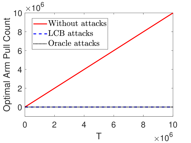
Refer to caption
Figure 6: Number of rounds the optimal arm was pulled using UCB algorithm

To further compare the performance of UCB and MOUCB, in Figure 6, we illustrate the performance of UCB algorithm for the three scenarios discussed above: under LCB attack, under oracle attack and under no attack. The results show that both LCB and oracle attacks can successfully manipulates the UCB algorithm into pulling a non-optimal arm very frequently, as the curves for the LCB attack and oracle attack are far away from the curve for no attack. This is in sharp contrast with the situation for MOUCB algorithm shown in Figure 5, where the all curves are almost identical.
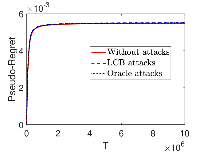
Refer to caption
Figure 7: Pseudo-regret of MOUCB algorithm
Refer to caption
Figure 8: Pseudo-regret of UCB algorithm

Figure 7 and Figure 8 illustrate the pseudo-regret of MOUCB bandit algorithm and UCB bandit algorithm respectively. In Figure 7, as predicted in our analysis, MOUCB algorithm archives logarithmic pseudo-regrets under both LCB attacks and the oracle attacks. Furthermore, the curves under both attacks are very close to that of the case without attacks. However, as shown in Figure 8, the pseudo-regret of UCB grows linearly under both attacks, while grows logarithmically under no attack. The figures again show that UCB is vulnerable to action-manipulation attacks while the proposed MOUCB is robust to the attacks (even for oracle attacks).

VI Conclusion

In this paper, we have introduced a new class of attacks on stochastic bandits: action-manipulation attacks. We have analyzed the attack against on the UCB algorithm and proved that the proposed LCB attack scheme can force the user to almost always pull a non-worst arm with only logarithm effort. To defend against this type of attacks, we have further designed a new bandit algorithm MOUCB that is robust to action-manipulation attacks. We have analyzed the regret of MOUCB under any attack with bounded cost, and have showed that the proposed algorithm is robust to the action-manipulation attacks.

Appendix A Proof of Lemma 2

The proof is similar with the proof of Lemma 1 that was proved in [22]. Let {Xj}j=1superscriptsubscriptsubscript𝑋𝑗𝑗1\{X_{j}\}_{j=1}^{\infty} be a sequence of i.i.dformulae-sequence𝑖𝑖𝑑i.i.d σ2superscript𝜎2\sigma^{2}-sub-Gaussian random variables with mean μ𝜇\mu. Let μ^0(t)=1N(t)j=1N(t)Xjsuperscript^𝜇0𝑡1𝑁𝑡superscriptsubscript𝑗1𝑁𝑡subscript𝑋𝑗\hat{\mu}^{0}(t)=\frac{1}{N(t)}\sum_{j=1}^{N(t)}X_{j}. By Hoeffding’s inequality.

(|μ^0(t)μ|η)2exp(N(t)η22σ2).superscript^𝜇0𝑡𝜇𝜂2𝑁𝑡superscript𝜂22superscript𝜎2\mathbb{P}(|\hat{\mu}^{0}(t)-\mu|\geq\eta)\leq 2\exp\left(-\frac{N(t)\eta^{2}}{2\sigma^{2}}\right). (24)

In order to ensure that 2subscript2\mathcal{E}_{2} holds for all arm i𝑖i, all arm j𝑗j and all pull counts N=Ni,j(t)𝑁subscript𝑁𝑖𝑗𝑡N=N_{i,j}(t), we set δi,j,N:=6δπ2K2N2assignsubscript𝛿𝑖𝑗𝑁6𝛿superscript𝜋2superscript𝐾2superscript𝑁2\delta_{i,j,N}:=\frac{6\delta}{\pi^{2}K^{2}N^{2}}. We have

(i,j,N:|μ^i,j(t)μj|2σ2Nlogπ2K2N23δ)=i=1Kj=1KN=1δi,N=δ.\begin{split}&\mathbb{P}\left(\exists i,\exists j,\exists N:|\hat{\mu}_{i,j}(t)-\mu_{j}|\geq\sqrt{\frac{2\sigma^{2}}{N}\log\frac{\pi^{2}K^{2}N^{2}}{3\delta}}\right)\\ &=\sum_{i=1}^{K}\sum_{j=1}^{K}\sum_{N=1}^{\infty}\delta_{i,N}=\delta.\end{split} (25)

Appendix B Proof of Lemma 3

According to event 2subscript2\mathcal{E}_{2}, we have

|μ^i(t)1Ni(t)sτi(t)μIs0|=|j=1KNi,j(t)Ni(t)(μ^i,j(t)μj)|j=1KNi,j(t)Ni(t)|μ^i,j(t)μj|<1Ni(t)j=1K2σ2Ni,j(t)logπ2K2(Ni,j(t))23δ.subscript^𝜇𝑖𝑡1subscript𝑁𝑖𝑡subscript𝑠subscript𝜏𝑖𝑡subscript𝜇superscriptsubscript𝐼𝑠0superscriptsubscript𝑗1𝐾subscript𝑁𝑖𝑗𝑡subscript𝑁𝑖𝑡subscript^𝜇𝑖𝑗𝑡subscript𝜇𝑗superscriptsubscript𝑗1𝐾subscript𝑁𝑖𝑗𝑡subscript𝑁𝑖𝑡subscript^𝜇𝑖𝑗𝑡subscript𝜇𝑗1subscript𝑁𝑖𝑡superscriptsubscript𝑗1𝐾2superscript𝜎2subscript𝑁𝑖𝑗𝑡superscript𝜋2superscript𝐾2superscriptsubscript𝑁𝑖𝑗𝑡23𝛿\begin{split}&\left|\hat{\mu}_{i}(t)-\frac{1}{N_{i}(t)}\sum_{s\in\tau_{i}(t)}\mu_{I_{s}^{0}}\right|\\ =&\left|\sum_{j=1}^{K}\frac{N_{i,j}(t)}{N_{i}(t)}\left(\hat{\mu}_{i,j}(t)-\mu_{j}\right)\right|\\ \leq&\sum_{j=1}^{K}\frac{N_{i,j}(t)}{N_{i}(t)}\left|\hat{\mu}_{i,j}(t)-\mu_{j}\right|\\ <&\frac{1}{N_{i}(t)}\sum_{j=1}^{K}\sqrt{2\sigma^{2}N_{i,j}(t)\log\frac{\pi^{2}K^{2}(N_{i,j}(t))^{2}}{3\delta}}.\end{split} (26)

Define a function f(N)=2σ2Nlogπ2K2N23δ::𝑓𝑁2superscript𝜎2𝑁superscript𝜋2superscript𝐾2superscript𝑁23𝛿\displaystyle f(N)=\sqrt{2\sigma^{2}N\log\frac{\pi^{2}K^{2}N^{2}}{3\delta}}:\mathbb{R}\to\mathbb{R}, and we have

f′′(N)=2N22σ2Nlogπ2K2N23δ=(2σ2logπ2K2N23δ)2+16σ44(2σ2Nlogπ2K2N23δ)32<0,superscript𝑓′′𝑁superscript2superscript𝑁22superscript𝜎2𝑁superscript𝜋2superscript𝐾2superscript𝑁23𝛿superscript2superscript𝜎2superscript𝜋2superscript𝐾2superscript𝑁23𝛿216superscript𝜎44superscript2superscript𝜎2𝑁superscript𝜋2superscript𝐾2superscript𝑁23𝛿320\begin{split}\displaystyle f^{\prime\prime}(N)=&\frac{\partial^{2}}{\partial N^{2}}\sqrt{2\sigma^{2}N\log\frac{\pi^{2}K^{2}N^{2}}{3\delta}}\\ =&-\frac{\left(2\sigma^{2}\log\frac{\pi^{2}K^{2}N^{2}}{3\delta}\right)^{2}+16\sigma^{4}}{4\left(2\sigma^{2}N\log\frac{\pi^{2}K^{2}N^{2}}{3\delta}\right)^{\frac{3}{2}}}\\ <&0,\end{split} (27)

when N1𝑁1N\geq 1.

Hence f𝑓\displaystyle f is strictly concave when N1𝑁1N\geq 1, and we have

j=1Kf(Ni,j(t))<Kf(1Kj=1KNi,j(t))=Kf(Ni(t)K).superscriptsubscript𝑗1𝐾𝑓subscript𝑁𝑖𝑗𝑡𝐾𝑓1𝐾superscriptsubscript𝑗1𝐾subscript𝑁𝑖𝑗𝑡𝐾𝑓subscript𝑁𝑖𝑡𝐾\begin{split}\displaystyle\sum_{j=1}^{K}f(N_{i,j}(t))<Kf\left(\frac{1}{K}\sum_{j=1}^{K}N_{i,j}(t)\right)=Kf\left(\frac{N_{i}(t)}{K}\right).\end{split} (28)

Thus,

|μ^i(t)1Ni(t)sτi(t)μIs0|<1Ni(t)K2σ2Ni(t)Klogπ2K2(Ni(t)K)23δ=2σ2KNi(t)logπ2(Ni(t))23δ.subscript^𝜇𝑖𝑡1subscript𝑁𝑖𝑡subscript𝑠subscript𝜏𝑖𝑡subscript𝜇superscriptsubscript𝐼𝑠01subscript𝑁𝑖𝑡𝐾2superscript𝜎2subscript𝑁𝑖𝑡𝐾superscript𝜋2superscript𝐾2superscriptsubscript𝑁𝑖𝑡𝐾23𝛿2superscript𝜎2𝐾subscript𝑁𝑖𝑡superscript𝜋2superscriptsubscript𝑁𝑖𝑡23𝛿\begin{split}&\left|\hat{\mu}_{i}(t)-\frac{1}{N_{i}(t)}\sum_{s\in\tau_{i}(t)}\mu_{I_{s}^{0}}\right|\\ <&\frac{1}{N_{i}(t)}K\sqrt{2\sigma^{2}\frac{N_{i}(t)}{K}\log\frac{\pi^{2}K^{2}\left(\frac{N_{i}(t)}{K}\right)^{2}}{3\delta}}\\ =&\sqrt{\frac{2\sigma^{2}K}{N_{i}(t)}\log\frac{\pi^{2}(N_{i}(t))^{2}}{3\delta}}.\end{split} (29)

Appendix C Proof of Lemma 4

The LCB attack scheme uses lower confidence bound to exploit the worst arm, so we need to prove that the attacker’s pull counts of all non-worst arms should be limited at round t𝑡t.

Consider the case that in round t+1𝑡1t+1, the user chooses a non-target arm It+1=iKsubscript𝐼𝑡1𝑖𝐾I_{t+1}=i\neq K and the attacker changes it to a non-worst arm It+10=jiWsuperscriptsubscript𝐼𝑡10𝑗subscript𝑖𝑊I_{t+1}^{0}=j\neq i_{W}. On one hand, under event 1subscript1\mathcal{E}_{1}, we have

μ^iW0(t)μiW<CB(NiW0(t)),andμ^j0(t)μj>CB(Nj0(t)).formulae-sequencesuperscriptsubscript^𝜇subscript𝑖𝑊0𝑡subscript𝜇subscript𝑖𝑊CBsuperscriptsubscript𝑁subscript𝑖𝑊0𝑡andsuperscriptsubscript^𝜇𝑗0𝑡subscript𝜇𝑗CBsuperscriptsubscript𝑁𝑗0𝑡\begin{split}&\hat{\mu}_{i_{W}}^{0}(t)-\mu_{i_{W}}<\textbf{CB}(N_{i_{W}}^{0}(t)),\\ \text{and}\ &\hat{\mu}_{j}^{0}(t)-\mu_{j}>-\textbf{CB}(N_{j}^{0}(t)).\end{split} (30)

On the other hand, according to the attack scheme, it must be the case that

μ^iW0(t)CB(NiW0(t))>μ^j0(t)CB(Nj0(t)),superscriptsubscript^𝜇subscript𝑖𝑊0𝑡CBsuperscriptsubscript𝑁subscript𝑖𝑊0𝑡superscriptsubscript^𝜇𝑗0𝑡CBsuperscriptsubscript𝑁𝑗0𝑡\begin{split}\hat{\mu}_{i_{W}}^{0}(t)-\textbf{CB}(N_{i_{W}}^{0}(t))>\hat{\mu}_{j}^{0}(t)-\textbf{CB}(N_{j}^{0}(t)),\end{split} (31)

which is equivalent to

CB(Nj0(t))>μ^j0(t)(μ^iW0(t)CB(NiW0(t))).CBsuperscriptsubscript𝑁𝑗0𝑡superscriptsubscript^𝜇𝑗0𝑡superscriptsubscript^𝜇subscript𝑖𝑊0𝑡CBsuperscriptsubscript𝑁subscript𝑖𝑊0𝑡\begin{split}\textbf{CB}(N_{j}^{0}(t))>\hat{\mu}_{j}^{0}(t)-(\hat{\mu}_{i_{W}}^{0}(t)-\textbf{CB}(N_{i_{W}}^{0}(t))).\end{split} (32)

Combining (32) with (30), we have

CB(Nj0(t))>μjCB(Nj0(t))μiWandCB(Nj0(t))>Δj,iW2.CBsuperscriptsubscript𝑁𝑗0𝑡subscript𝜇𝑗CBsuperscriptsubscript𝑁𝑗0𝑡subscript𝜇subscript𝑖𝑊andCBsuperscriptsubscript𝑁𝑗0𝑡subscriptΔ𝑗subscript𝑖𝑊2\begin{split}&\textbf{CB}(N_{j}^{0}(t))>\mu_{j}-\textbf{CB}(N_{j}^{0}(t))-\mu_{i_{W}}\\ \text{and}\ &\textbf{CB}(N_{j}^{0}(t))>\frac{\Delta_{j,i_{W}}}{2}.\end{split} (33)

Using on the fact that Nj0(t)tsuperscriptsubscript𝑁𝑗0𝑡𝑡N_{j}^{0}(t)\leq t and Ni,j(t)Nj0(t)subscript𝑁𝑖𝑗𝑡superscriptsubscript𝑁𝑗0𝑡N_{i,j}(t)\leq N_{j}^{0}(t), we have

Δj,iW2<CB(Nj0(t))=2σ2Nj0(t)logπ2K(Nj0(t))23δ2σ2Nj0(t)logπ2Kt23δ2σ2Ni,j(t)logπ2Kt23δ,subscriptΔ𝑗subscript𝑖𝑊2CBsuperscriptsubscript𝑁𝑗0𝑡2superscript𝜎2superscriptsubscript𝑁𝑗0𝑡superscript𝜋2𝐾superscriptsuperscriptsubscript𝑁𝑗0𝑡23𝛿2superscript𝜎2superscriptsubscript𝑁𝑗0𝑡superscript𝜋2𝐾superscript𝑡23𝛿2superscript𝜎2subscript𝑁𝑖𝑗𝑡superscript𝜋2𝐾superscript𝑡23𝛿\begin{split}\frac{\Delta_{j,i_{W}}}{2}<&\textbf{CB}(N_{j}^{0}(t))\\ =&\sqrt{\frac{2\sigma^{2}}{N_{j}^{0}(t)}\log\frac{\pi^{2}K(N_{j}^{0}(t))^{2}}{3\delta}}\\ \leq&\sqrt{\frac{2\sigma^{2}}{N_{j}^{0}(t)}\log\frac{\pi^{2}Kt^{2}}{3\delta}}\\ \leq&\sqrt{\frac{2\sigma^{2}}{N_{i,j}(t)}\log\frac{\pi^{2}Kt^{2}}{3\delta}},\end{split} (34)

which is equivalent to

Ni,j(t)<8σ2Δj,iW2logπ2Kt23δ.subscript𝑁𝑖𝑗𝑡8superscript𝜎2superscriptsubscriptΔ𝑗subscript𝑖𝑊2superscript𝜋2𝐾superscript𝑡23𝛿\begin{split}N_{i,j}(t)<\frac{8\sigma^{2}}{\Delta_{j,i_{W}}^{2}}\log\frac{\pi^{2}Kt^{2}}{3\delta}.\end{split} (35)

Hence, under event 2subscript2\mathcal{E}_{2}, we have

μ^i(t)<1Ni(t)sτi(t)μIs0+2σ2KNi(t)logπ2(Ni(t))23δ=1Ni(t)jsτi,j(t)μIs0+2σ2KNi(t)logπ2(Ni(t))23δ=1Ni(t)jNi,j(t)μj+2σ2KNi(t)logπ2(Ni(t))23δ=jNi,j(t)Ni(t)(Δj,iW+μiW)+2σ2KNi(t)logπ2(Ni(t))23δ<μiW+2σ2KNi(t)logπ2(Ni(t))23δ+1Ni(t)jiW8σ2Δj,iWlogπ2Kt23δ.subscript^𝜇𝑖𝑡1subscript𝑁𝑖𝑡subscript𝑠subscript𝜏𝑖𝑡subscript𝜇superscriptsubscript𝐼𝑠02superscript𝜎2𝐾subscript𝑁𝑖𝑡superscript𝜋2superscriptsubscript𝑁𝑖𝑡23𝛿1subscript𝑁𝑖𝑡subscript𝑗subscript𝑠subscript𝜏𝑖𝑗𝑡subscript𝜇superscriptsubscript𝐼𝑠02superscript𝜎2𝐾subscript𝑁𝑖𝑡superscript𝜋2superscriptsubscript𝑁𝑖𝑡23𝛿1subscript𝑁𝑖𝑡subscript𝑗subscript𝑁𝑖𝑗𝑡subscript𝜇𝑗2superscript𝜎2𝐾subscript𝑁𝑖𝑡superscript𝜋2superscriptsubscript𝑁𝑖𝑡23𝛿subscript𝑗subscript𝑁𝑖𝑗𝑡subscript𝑁𝑖𝑡subscriptΔ𝑗subscript𝑖𝑊subscript𝜇subscript𝑖𝑊2superscript𝜎2𝐾subscript𝑁𝑖𝑡superscript𝜋2superscriptsubscript𝑁𝑖𝑡23𝛿subscript𝜇subscript𝑖𝑊2superscript𝜎2𝐾subscript𝑁𝑖𝑡superscript𝜋2superscriptsubscript𝑁𝑖𝑡23𝛿1subscript𝑁𝑖𝑡subscript𝑗subscript𝑖𝑊8superscript𝜎2subscriptΔ𝑗subscript𝑖𝑊superscript𝜋2𝐾superscript𝑡23𝛿\begin{split}\hat{\mu}_{i}(t)<&\frac{1}{N_{i}(t)}\sum_{s\in\tau_{i}(t)}\mu_{I_{s}^{0}}+\sqrt{\frac{2\sigma^{2}K}{N_{i}(t)}\log\frac{\pi^{2}(N_{i}(t))^{2}}{3\delta}}\\ =&\frac{1}{N_{i}(t)}\sum_{j}\sum_{s\in\tau_{i,j}(t)}\mu_{I_{s}^{0}}+\sqrt{\frac{2\sigma^{2}K}{N_{i}(t)}\log\frac{\pi^{2}(N_{i}(t))^{2}}{3\delta}}\\ =&\frac{1}{N_{i}(t)}\sum_{j}N_{i,j}(t)\mu_{j}+\sqrt{\frac{2\sigma^{2}K}{N_{i}(t)}\log\frac{\pi^{2}(N_{i}(t))^{2}}{3\delta}}\\ =&\sum_{j}\frac{N_{i,j}(t)}{N_{i}(t)}(\Delta_{j,i_{W}}+\mu_{i_{W}})+\sqrt{\frac{2\sigma^{2}K}{N_{i}(t)}\log\frac{\pi^{2}(N_{i}(t))^{2}}{3\delta}}\\ <&\mu_{i_{W}}+\sqrt{\frac{2\sigma^{2}K}{N_{i}(t)}\log\frac{\pi^{2}(N_{i}(t))^{2}}{3\delta}}\\ &+\frac{1}{N_{i}(t)}\sum_{j\neq i_{W}}\frac{8\sigma^{2}}{\Delta_{j,i_{W}}}\log\frac{\pi^{2}Kt^{2}}{3\delta}.\end{split} (36)

The lemma is proved.

Appendix D Proof of Theorem 1

By inferring from Lemma 1, we have that with probability 1δK1𝛿𝐾1-\frac{\delta}{K}, t>K:|μ^K0(t)μK|<CB(NK0(t)):for-all𝑡𝐾superscriptsubscript^𝜇𝐾0𝑡subscript𝜇𝐾CBsuperscriptsubscript𝑁𝐾0𝑡\forall t>K:|\hat{\mu}_{K}^{0}(t)-\mu_{K}|<\textbf{CB}(N_{K}^{0}(t)).

Because the LCB attack scheme does not attack the target arm, we can also conclude that with probability 1δK1𝛿𝐾1-\frac{\delta}{K}, t>K:|μ^K(t)μK|<CB(NK(t)):for-all𝑡𝐾subscript^𝜇𝐾𝑡subscript𝜇𝐾CBsubscript𝑁𝐾𝑡\forall t>K:|\hat{\mu}_{K}(t)-\mu_{K}|<\textbf{CB}(N_{K}(t)).

The user relies on the UCB algorithm to choose arms. If at round t𝑡t, the user chooses an arm It=iKsubscript𝐼𝑡𝑖𝐾I_{t}=i\neq K, which is not the target arm, we have

μ^i(t1)+3σlogtNi(t1)>μ^K(t1)+3σlogtNK(t1),subscript^𝜇𝑖𝑡13𝜎𝑡subscript𝑁𝑖𝑡1subscript^𝜇𝐾𝑡13𝜎𝑡subscript𝑁𝐾𝑡1\begin{split}\hat{\mu}_{i}(t-1)+3\sigma\sqrt{\frac{\log t}{N_{i}(t-1)}}>\hat{\mu}_{K}(t-1)+3\sigma\sqrt{\frac{\log t}{N_{K}(t-1)}},\end{split} (37)

which is equivalent to

3σlogtNi(t1)>μ^i(t1)+μ^K(t1)+3σlogtNK(t1).3𝜎𝑡subscript𝑁𝑖𝑡1subscript^𝜇𝑖𝑡1subscript^𝜇𝐾𝑡13𝜎𝑡subscript𝑁𝐾𝑡1\begin{split}3\sigma\sqrt{\frac{\log t}{N_{i}(t-1)}}>-\hat{\mu}_{i}(t-1)+\hat{\mu}_{K}(t-1)+3\sigma\sqrt{\frac{\log t}{N_{K}(t-1)}}.\end{split} (38)

Under event 1subscript1\mathcal{E}_{1}, we have

μ^K(t)>μKCB(NK(t)).subscript^𝜇𝐾𝑡subscript𝜇𝐾CBsubscript𝑁𝐾𝑡\begin{split}\hat{\mu}_{K}(t)>\mu_{K}-\textbf{CB}(N_{K}(t)).\end{split} (39)

Under event 12subscript1subscript2\mathcal{E}_{1}\cap\mathcal{E}_{2}, according to Lemma 4, we have

μ^i(t)μiW+2σ2KNi(t)logπ2(Ni(t))23δ+1Ni(t)jiW8σ2Δj,iWlogπ2Kt23δ.subscript^𝜇𝑖𝑡subscript𝜇subscript𝑖𝑊2superscript𝜎2𝐾subscript𝑁𝑖𝑡superscript𝜋2superscriptsubscript𝑁𝑖𝑡23𝛿1subscript𝑁𝑖𝑡subscript𝑗subscript𝑖𝑊8superscript𝜎2subscriptΔ𝑗subscript𝑖𝑊superscript𝜋2𝐾superscript𝑡23𝛿\begin{split}\hat{\mu}_{i}(t)\leq\mu_{i_{W}}&+\sqrt{\frac{2\sigma^{2}K}{N_{i}(t)}\log\frac{\pi^{2}(N_{i}(t))^{2}}{3\delta}}\\ &+\frac{1}{N_{i}(t)}\sum_{j\neq i_{W}}\frac{8\sigma^{2}}{\Delta_{j,i_{W}}}\log\frac{\pi^{2}Kt^{2}}{3\delta}.\end{split} (40)

Combing the inequalities above,

3σlogtNi(t1)>μiW2σ2KNi(t1)logπ2(Ni(t1))23δ1Ni(t1)jiW8σ2Δj,iWlogπ2K(t1)23δ+μKCB(NK(t1))+3σlogtNK(t1).3𝜎𝑡subscript𝑁𝑖𝑡1subscript𝜇subscript𝑖𝑊2superscript𝜎2𝐾subscript𝑁𝑖𝑡1superscript𝜋2superscriptsubscript𝑁𝑖𝑡123𝛿1subscript𝑁𝑖𝑡1subscript𝑗subscript𝑖𝑊8superscript𝜎2subscriptΔ𝑗subscript𝑖𝑊superscript𝜋2𝐾superscript𝑡123𝛿subscript𝜇𝐾CBsubscript𝑁𝐾𝑡13𝜎𝑡subscript𝑁𝐾𝑡1\begin{split}3\sigma\sqrt{\frac{\log t}{N_{i}(t-1)}}&>-\mu_{i_{W}}-\sqrt{\frac{2\sigma^{2}K}{N_{i}(t-1)}\log\frac{\pi^{2}(N_{i}(t-1))^{2}}{3\delta}}\\ &-\frac{1}{N_{i}(t-1)}\sum_{j\neq i_{W}}\frac{8\sigma^{2}}{\Delta_{j,i_{W}}}\log\frac{\pi^{2}K(t-1)^{2}}{3\delta}\\ &+\mu_{K}-\textbf{CB}(N_{K}(t-1))+3\sigma\sqrt{\frac{\log t}{N_{K}(t-1)}}.\end{split} (41)

When t(π2K3δ)25𝑡superscriptsuperscript𝜋2𝐾3𝛿25t\geq(\frac{\pi^{2}K}{3\delta})^{\frac{2}{5}},

3σlogtNK(t1)4σ2logtNK(t1)+5σ2log(π2K3δ)25NK(t1)2σ2logπ2Kt23δNK(t1)2σ2logπ2K(NK(t1))23δNK(t1)=CB(NK(t1)).\begin{split}3\sigma\sqrt{\frac{\log t}{N_{K}(t-1)}}&\geq\sqrt{4\sigma^{2}\frac{\log t}{N_{K}(t-1)}+5\sigma^{2}\frac{\log(\frac{\pi^{2}K}{3\delta})^{\frac{2}{5}}}{N_{K}(t-1)}}\\ &\geq\sqrt{2\sigma^{2}\frac{\log\frac{\pi^{2}Kt^{2}}{3\delta}}{N_{K}(t-1)}}\\ &\geq\sqrt{2\sigma^{2}\frac{\log\frac{\pi^{2}K(N_{K}(t-1))^{2}}{3\delta}}{N_{K}(t-1)}}\\ &=\textbf{CB}(N_{K}(t-1)).\end{split} (42)

Now the inequality only depends on Ni(t1)subscript𝑁𝑖𝑡1N_{i}(t-1) and some constants:

3σlogtNi(t1)>ΔK,iW2σ2KNi(t1)logπ2(Ni(t1))23δ1Ni(t1)jiW8σ2Δj,iWlogπ2K(t1)23δ>ΔK,iW2σ2KNi(t1)logπ2t23δ1Ni(t1)jiW8σ2Δj,iWlogπ2Kt23δ.3𝜎𝑡subscript𝑁𝑖𝑡1subscriptΔ𝐾subscript𝑖𝑊2superscript𝜎2𝐾subscript𝑁𝑖𝑡1superscript𝜋2superscriptsubscript𝑁𝑖𝑡123𝛿1subscript𝑁𝑖𝑡1subscript𝑗subscript𝑖𝑊8superscript𝜎2subscriptΔ𝑗subscript𝑖𝑊superscript𝜋2𝐾superscript𝑡123𝛿subscriptΔ𝐾subscript𝑖𝑊2superscript𝜎2𝐾subscript𝑁𝑖𝑡1superscript𝜋2superscript𝑡23𝛿1subscript𝑁𝑖𝑡1subscript𝑗subscript𝑖𝑊8superscript𝜎2subscriptΔ𝑗subscript𝑖𝑊superscript𝜋2𝐾superscript𝑡23𝛿\begin{split}3\sigma\sqrt{\frac{\log t}{N_{i}(t-1)}}>&\Delta_{K,i_{W}}-\sqrt{\frac{2\sigma^{2}K}{N_{i}(t-1)}\log\frac{\pi^{2}(N_{i}(t-1))^{2}}{3\delta}}\\ &-\frac{1}{N_{i}(t-1)}\sum_{j\neq i_{W}}\frac{8\sigma^{2}}{\Delta_{j,i_{W}}}\log\frac{\pi^{2}K(t-1)^{2}}{3\delta}\\ >&\Delta_{K,i_{W}}-\sqrt{\frac{2\sigma^{2}K}{N_{i}(t-1)}\log\frac{\pi^{2}t^{2}}{3\delta}}\\ &-\frac{1}{N_{i}(t-1)}\sum_{j\neq i_{W}}\frac{8\sigma^{2}}{\Delta_{j,i_{W}}}\log\frac{\pi^{2}Kt^{2}}{3\delta}.\end{split} (43)

By solving the inequality above, we have:

Ni(t1)<14ΔK,iW2(3σlogt+2σ2Klogπ2t23δ+((3σlogt+2σ2Klogπ2t23δ)2+4ΔK,iWjiW8σ2Δj,iWlogπ2Kt23δ)12)2.subscript𝑁𝑖𝑡114superscriptsubscriptΔ𝐾subscript𝑖𝑊2superscript3𝜎𝑡2superscript𝜎2𝐾superscript𝜋2superscript𝑡23𝛿superscriptsuperscript3𝜎𝑡2superscript𝜎2𝐾superscript𝜋2superscript𝑡23𝛿24subscriptΔ𝐾subscript𝑖𝑊subscript𝑗subscript𝑖𝑊8superscript𝜎2subscriptΔ𝑗subscript𝑖𝑊superscript𝜋2𝐾superscript𝑡23𝛿122\begin{split}N_{i}(t-1)<&\frac{1}{4\Delta_{K,i_{W}}^{2}}\left(3\sigma\sqrt{\log t}+\sqrt{2\sigma^{2}K\log\frac{\pi^{2}t^{2}}{3\delta}}\right.\\ &+\left(\left(3\sigma\sqrt{\log t}+\sqrt{2\sigma^{2}K\log\frac{\pi^{2}t^{2}}{3\delta}}\right)^{2}\right.\\ &\left.\left.+4\Delta_{K,i_{W}}\sum_{j\neq i_{W}}\frac{8\sigma^{2}}{\Delta_{j,i_{W}}}\log\frac{\pi^{2}Kt^{2}}{3\delta}\right)^{\frac{1}{2}}\right)^{2}.\end{split} (44)

Since event 12subscript1subscript2\mathcal{E}_{1}\cap\mathcal{E}_{2} occurs with probability at least 12δ12𝛿1-2\delta, we have that (44) holds with probability at least 12δ12𝛿1-2\delta. Theorem 1 follows immediately from the definition of the attack cost and (44).

Appendix E Proof of Theorem 2

Because the target arm is the worst arm, the mean rewards of all arms are larger than or equal to that of the target arm. Thus, for any attack scheme, we have

1Ni(t)sτi(t)μIs0μK.1subscript𝑁𝑖𝑡subscript𝑠subscript𝜏𝑖𝑡subscript𝜇superscriptsubscript𝐼𝑠0subscript𝜇𝐾\frac{1}{N_{i}(t)}\sum_{s\in\tau_{i}(t)}\mu_{I_{s}^{0}}\geq\mu_{K}. (45)

If the user pulls arm K𝐾K at round t𝑡t, according to UCB algorithm, we have for any arm iK𝑖𝐾i\neq K,

μ^i(t1)+3σlogtNi(t1)<μ^K(t1)+3σlogtNK(t1).subscript^𝜇𝑖𝑡13𝜎𝑡subscript𝑁𝑖𝑡1subscript^𝜇𝐾𝑡13𝜎𝑡subscript𝑁𝐾𝑡1\begin{split}\hat{\mu}_{i}(t-1)+3\sigma\sqrt{\frac{\log t}{N_{i}(t-1)}}<\hat{\mu}_{K}(t-1)+3\sigma\sqrt{\frac{\log t}{N_{K}(t-1)}}.\end{split} (46)

Under event 2subscript2\mathcal{E}_{2}, we have Lemma 3 and (29) holds for all arm i𝑖i, which implies

μ^i(t1)>1Ni(t1)sτi(t1)μIs02σ2KNi(t1)logπ2(Ni(t1))23δ,subscript^𝜇𝑖𝑡11subscript𝑁𝑖𝑡1subscript𝑠subscript𝜏𝑖𝑡1subscript𝜇superscriptsubscript𝐼𝑠02superscript𝜎2𝐾subscript𝑁𝑖𝑡1superscript𝜋2superscriptsubscript𝑁𝑖𝑡123𝛿\begin{split}\hat{\mu}_{i}(t-1)>&\frac{1}{N_{i}(t-1)}\sum_{s\in\tau_{i}(t-1)}\mu_{I_{s}^{0}}-\\ &\sqrt{\frac{2\sigma^{2}K}{N_{i}(t-1)}\log\frac{\pi^{2}(N_{i}(t-1))^{2}}{3\delta}},\end{split} (47)

and

μ^K(t1)<1NK(t1)sτK(t1)μIs0+2σ2KNK(t1)logπ2(NK(t1))23δ.subscript^𝜇𝐾𝑡11subscript𝑁𝐾𝑡1subscript𝑠subscript𝜏𝐾𝑡1subscript𝜇superscriptsubscript𝐼𝑠02superscript𝜎2𝐾subscript𝑁𝐾𝑡1superscript𝜋2superscriptsubscript𝑁𝐾𝑡123𝛿\begin{split}\hat{\mu}_{K}(t-1)<&\frac{1}{N_{K}(t-1)}\sum_{s\in\tau_{K}(t-1)}\mu_{I_{s}^{0}}+\\ &\sqrt{\frac{2\sigma^{2}K}{N_{K}(t-1)}\log\frac{\pi^{2}(N_{K}(t-1))^{2}}{3\delta}}.\end{split} (48)

Noted that for δ>12𝛿12\delta>\frac{1}{2}, h(N)=2σ2NKlogπ2N23δ::𝑁2superscript𝜎2𝑁𝐾superscript𝜋2superscript𝑁23𝛿\displaystyle h(N)=2\sigma^{2}\frac{N}{K}\log\frac{\pi^{2}N^{2}}{3\delta}:\mathbb{R}\to\mathbb{R} is monotonically decreasing in N1𝑁1N\geq 1.

If Ni(t1)<116NK(t1)subscript𝑁𝑖𝑡1116subscript𝑁𝐾𝑡1N_{i}(t-1)<\frac{1}{16}N_{K}(t-1) and Ni(t1)<3δπt964Ksubscript𝑁𝑖𝑡13𝛿𝜋superscript𝑡964𝐾N_{i}(t-1)<\frac{\sqrt{3\delta}}{\pi}t^{\frac{9}{64K}} hold for any arm i𝑖i, we have

3σlogtNK(t1)<34σlogtNi(t1),3𝜎𝑡subscript𝑁𝐾𝑡134𝜎𝑡subscript𝑁𝑖𝑡1\begin{split}3\sigma\sqrt{\frac{\log t}{N_{K}(t-1)}}<\frac{3}{4}\sigma\sqrt{\frac{\log t}{N_{i}(t-1)}},\end{split} (49)

and

2σ2KNK(t1)logπ2(NK(t1))23δ<2σ2KNi(t1)logπ2(Ni(t1))23δ<34σlogtNi(t1).2superscript𝜎2𝐾subscript𝑁𝐾𝑡1superscript𝜋2superscriptsubscript𝑁𝐾𝑡123𝛿2superscript𝜎2𝐾subscript𝑁𝑖𝑡1superscript𝜋2superscriptsubscript𝑁𝑖𝑡123𝛿34𝜎𝑡subscript𝑁𝑖𝑡1\begin{split}&\sqrt{\frac{2\sigma^{2}K}{N_{K}(t-1)}\log\frac{\pi^{2}(N_{K}(t-1))^{2}}{3\delta}}\\ <&\sqrt{\frac{2\sigma^{2}K}{N_{i}(t-1)}\log\frac{\pi^{2}(N_{i}(t-1))^{2}}{3\delta}}\\ <&\frac{3}{4}\sigma\sqrt{\frac{\log t}{N_{i}(t-1)}}.\end{split} (50)

Combining the inequalities above, we find

34σlogtNi(t1)<1NK(t1)sτK(t1)μIs0μK.34𝜎𝑡subscript𝑁𝑖𝑡11subscript𝑁𝐾𝑡1subscript𝑠subscript𝜏𝐾𝑡1subscript𝜇superscriptsubscript𝐼𝑠0subscript𝜇𝐾\begin{split}\frac{3}{4}\sigma\sqrt{\frac{\log t}{N_{i}(t-1)}}<\frac{1}{N_{K}(t-1)}\sum_{s\in\tau_{K}(t-1)}\mu_{I_{s}^{0}}-\mu_{K}.\end{split} (51)

Since the attack cost is limited in 𝒪(logt)𝒪𝑡\mathcal{O}(\log t),

1NK(t1)sτK(t1)μIs0μK=𝒪(logt)NK(t1),1subscript𝑁𝐾𝑡1subscript𝑠subscript𝜏𝐾𝑡1subscript𝜇superscriptsubscript𝐼𝑠0subscript𝜇𝐾𝒪𝑡subscript𝑁𝐾𝑡1\begin{split}\frac{1}{N_{K}(t-1)}\sum_{s\in\tau_{K}(t-1)}\mu_{I_{s}^{0}}-\mu_{K}=\frac{\mathcal{O}(\log t)}{N_{K}(t-1)},\end{split} (52)

so

Ni(t1)=Ω(σ(NK(t1))2).subscript𝑁𝑖𝑡1Ω𝜎superscriptsubscript𝑁𝐾𝑡12\begin{split}N_{i}(t-1)=\Omega(\sigma(N_{K}(t-1))^{2}).\end{split} (53)

In summary, as long as the event 2subscript2\mathcal{E}_{2} holds, at least one of the three following equations must be true:

Ni(t1)=Ω(σ(NK(t1))2),Ni(t1)116NK(t1),Ni(t1)3δπt964K.formulae-sequencesubscript𝑁𝑖𝑡1Ω𝜎superscriptsubscript𝑁𝐾𝑡12formulae-sequencesubscript𝑁𝑖𝑡1116subscript𝑁𝐾𝑡1subscript𝑁𝑖𝑡13𝛿𝜋superscript𝑡964𝐾\begin{split}&N_{i}(t-1)=\Omega(\sigma(N_{K}(t-1))^{2}),\\ &N_{i}(t-1)\geq\frac{1}{16}N_{K}(t-1),\\ &N_{i}(t-1)\geq\frac{\sqrt{3\delta}}{\pi}t^{\frac{9}{64K}}.\end{split} (54)

In addition, any one of the three equations shows that the user pulls the non-target arm more than 𝒪(tα)𝒪superscript𝑡𝛼\mathcal{O}(t^{\alpha}) times, in which α<964K𝛼964𝐾\alpha<\frac{9}{64K}. Since event 2subscript2\mathcal{E}_{2} holds with probability at least 1δ1𝛿1-\delta, the conclusion in the Theorem holds with probability at least 1δ1𝛿1-\delta.

Appendix F Proof of Lemma 5

Note that for δ13𝛿13\delta\leq\frac{1}{3}, β(N)=2σ2KNlogπ2N23δ𝛽𝑁2superscript𝜎2𝐾𝑁superscript𝜋2superscript𝑁23𝛿\beta(N)=\sqrt{\frac{2\sigma^{2}K}{N}\log\frac{\pi^{2}N^{2}}{3\delta}} is monotonically decreasing in N𝑁N, as

Nβ2(N)=2σ2KN2(2logπ2N23δ)2σ2KN2(2logπ23δ)<0.𝑁superscript𝛽2𝑁2superscript𝜎2𝐾superscript𝑁22superscript𝜋2superscript𝑁23𝛿2superscript𝜎2𝐾superscript𝑁22superscript𝜋23𝛿0\begin{split}\frac{\partial}{\partial N}\beta^{2}(N)=&\frac{2\sigma^{2}K}{N^{2}}\left(2-\log\frac{\pi^{2}N^{2}}{3\delta}\right)\\ \leq&\frac{2\sigma^{2}K}{N^{2}}\left(2-\log\frac{\pi^{2}}{3\delta}\right)<0.\end{split} (55)

We first prove the first inequality in Lemma 5. Consider the optimal arm iOsubscript𝑖𝑂i_{O} and the worst arm iWsubscript𝑖𝑊i_{W}. Define Ci:=|{t:tT,It0It=i}|assignsubscript𝐶𝑖conditional-set𝑡formulae-sequence𝑡𝑇superscriptsubscript𝐼𝑡0subscript𝐼𝑡𝑖C_{i}:=|\{t:t\leq T,I_{t}^{0}\not=I_{t}=i\}|. In the action-manipulation setting, when t>2AK𝑡2𝐴𝐾t>2AK, MOUCB algorithm has

1NiO(t)sτiO(t)μIs0NiO(t)CiONiO(t)μiO+CiONiO(t)μiW=μiOΔiO,iWCiONiO(t)μiOΔiO,iWCiO2A,1subscript𝑁subscript𝑖𝑂𝑡subscript𝑠subscript𝜏subscript𝑖𝑂𝑡subscript𝜇superscriptsubscript𝐼𝑠0subscript𝑁subscript𝑖𝑂𝑡subscript𝐶subscript𝑖𝑂subscript𝑁subscript𝑖𝑂𝑡subscript𝜇subscript𝑖𝑂subscript𝐶subscript𝑖𝑂subscript𝑁subscript𝑖𝑂𝑡subscript𝜇subscript𝑖𝑊subscript𝜇subscript𝑖𝑂subscriptΔsubscript𝑖𝑂subscript𝑖𝑊subscript𝐶subscript𝑖𝑂subscript𝑁subscript𝑖𝑂𝑡subscript𝜇subscript𝑖𝑂subscriptΔsubscript𝑖𝑂subscript𝑖𝑊subscript𝐶subscript𝑖𝑂2𝐴\begin{split}\frac{1}{N_{i_{O}}(t)}\sum_{s\in\tau_{i_{O}}(t)}\mu_{I_{s}^{0}}&\geq\frac{N_{i_{O}}(t)-C_{i_{O}}}{N_{i_{O}}(t)}\mu_{i_{O}}+\frac{C_{i_{O}}}{N_{i_{O}}(t)}\mu_{i_{W}}\\ &=\mu_{i_{O}}-\Delta_{i_{O},i_{W}}\frac{C_{i_{O}}}{N_{i_{O}}(t)}\\ &\geq\mu_{i_{O}}-\Delta_{i_{O},i_{W}}\frac{C_{i_{O}}}{2A},\end{split} (56)

and

1NiW(t)sτiW(t)μIs0NiW(t)CiWNiW(t)μiW+CiWNiW(t)μiO=μiW+ΔiO,iWCiWNiW(t)μiW+ΔiO,iWCiW2A.1subscript𝑁subscript𝑖𝑊𝑡subscript𝑠subscript𝜏subscript𝑖𝑊𝑡subscript𝜇superscriptsubscript𝐼𝑠0subscript𝑁subscript𝑖𝑊𝑡subscript𝐶subscript𝑖𝑊subscript𝑁subscript𝑖𝑊𝑡subscript𝜇subscript𝑖𝑊subscript𝐶subscript𝑖𝑊subscript𝑁subscript𝑖𝑊𝑡subscript𝜇subscript𝑖𝑂subscript𝜇subscript𝑖𝑊subscriptΔsubscript𝑖𝑂subscript𝑖𝑊subscript𝐶subscript𝑖𝑊subscript𝑁subscript𝑖𝑊𝑡subscript𝜇subscript𝑖𝑊subscriptΔsubscript𝑖𝑂subscript𝑖𝑊subscript𝐶subscript𝑖𝑊2𝐴\begin{split}\frac{1}{N_{i_{W}}(t)}\sum_{s\in\tau_{i_{W}}(t)}\mu_{I_{s}^{0}}&\leq\frac{N_{i_{W}}(t)-C_{i_{W}}}{N_{i_{W}}(t)}\mu_{i_{W}}+\frac{C_{i_{W}}}{N_{i_{W}}(t)}\mu_{i_{O}}\\ &=\mu_{i_{W}}+\Delta_{i_{O},i_{W}}\frac{C_{i_{W}}}{N_{i_{W}}(t)}\\ &\leq\mu_{i_{W}}+\Delta_{i_{O},i_{W}}\frac{C_{i_{W}}}{2A}.\end{split} (57)

Combining (56) and (57), we have

1NiO(t)sτiO(t)μIs01NiW(t)sτiW(t)μIs0μiOμiWΔiO,iWCiW2AΔiO,iWCiO2AμiOμiWΔiO,iWA2A=ΔiO,iW2.1subscript𝑁subscript𝑖𝑂𝑡subscript𝑠subscript𝜏subscript𝑖𝑂𝑡subscript𝜇superscriptsubscript𝐼𝑠01subscript𝑁subscript𝑖𝑊𝑡subscript𝑠subscript𝜏subscript𝑖𝑊𝑡subscript𝜇superscriptsubscript𝐼𝑠0subscript𝜇subscript𝑖𝑂subscript𝜇subscript𝑖𝑊subscriptΔsubscript𝑖𝑂subscript𝑖𝑊subscript𝐶subscript𝑖𝑊2𝐴subscriptΔsubscript𝑖𝑂subscript𝑖𝑊subscript𝐶subscript𝑖𝑂2𝐴subscript𝜇subscript𝑖𝑂subscript𝜇subscript𝑖𝑊subscriptΔsubscript𝑖𝑂subscript𝑖𝑊𝐴2𝐴subscriptΔsubscript𝑖𝑂subscript𝑖𝑊2\begin{split}&\frac{1}{N_{i_{O}}(t)}\sum_{s\in\tau_{i_{O}}(t)}\mu_{I_{s}^{0}}-\frac{1}{N_{i_{W}}(t)}\sum_{s\in\tau_{i_{W}}(t)}\mu_{I_{s}^{0}}\\ \geq&\mu_{i_{O}}-\mu_{i_{W}}-\Delta_{i_{O},i_{W}}\frac{C_{i_{W}}}{2A}-\Delta_{i_{O},i_{W}}\frac{C_{i_{O}}}{2A}\\ \geq&\mu_{i_{O}}-\mu_{i_{W}}-\Delta_{i_{O},i_{W}}\frac{A}{2A}\\ =&\frac{\Delta_{i_{O},i_{W}}}{2}.\end{split} (58)

From (29), we could find

1NiO(t)sτiO(t)μIs01NiW(t)sτiW(t)μIs0μ^iO(t)+β(NiO(t))(μ^iW(t)β(NiW(t)))maxi,j{μ^i(t)+β(Ni(t))(μ^j(t)β(Nj(t)))}.1subscript𝑁subscript𝑖𝑂𝑡subscript𝑠subscript𝜏subscript𝑖𝑂𝑡subscript𝜇superscriptsubscript𝐼𝑠01subscript𝑁subscript𝑖𝑊𝑡subscript𝑠subscript𝜏subscript𝑖𝑊𝑡subscript𝜇superscriptsubscript𝐼𝑠0subscript^𝜇subscript𝑖𝑂𝑡𝛽subscript𝑁subscript𝑖𝑂𝑡subscript^𝜇subscript𝑖𝑊𝑡𝛽subscript𝑁subscript𝑖𝑊𝑡subscript𝑖𝑗subscript^𝜇𝑖𝑡𝛽subscript𝑁𝑖𝑡subscript^𝜇𝑗𝑡𝛽subscript𝑁𝑗𝑡\begin{split}&\frac{1}{N_{i_{O}}(t)}\sum_{s\in\tau_{i_{O}}(t)}\mu_{I_{s}^{0}}-\frac{1}{N_{i_{W}}(t)}\sum_{s\in\tau_{i_{W}}(t)}\mu_{I_{s}^{0}}\\ \leq&\hat{\mu}_{i_{O}}(t)+\beta(N_{i_{O}}(t))-(\hat{\mu}_{i_{W}}(t)-\beta(N_{i_{W}}(t)))\\ \leq&\max_{i,j}\left\{\hat{\mu}_{i}(t)+\beta(N_{i}(t))-\left(\hat{\mu}_{j}(t)-\beta\left(N_{j}(t)\right)\right)\right\}.\end{split} (59)

We now prove the second inequality in Lemma 5:

maxi,j{μ^i(t)+β(Ni(t))(μ^j(t)β(Nj(t)))}maxi,j{1Ni(t)sτi(t)μIs0+2β(Ni(t))(1Ni(t)sτi(t)μIs02β(Nj(t)))}ΔiO,iW+maxi,j{2β(Ni(t))+2β(Nj(t))}.subscript𝑖𝑗subscript^𝜇𝑖𝑡𝛽subscript𝑁𝑖𝑡subscript^𝜇𝑗𝑡𝛽subscript𝑁𝑗𝑡subscript𝑖𝑗1subscript𝑁𝑖𝑡subscript𝑠subscript𝜏𝑖𝑡subscript𝜇superscriptsubscript𝐼𝑠02𝛽subscript𝑁𝑖𝑡1subscript𝑁𝑖𝑡subscript𝑠subscript𝜏𝑖𝑡subscript𝜇superscriptsubscript𝐼𝑠02𝛽subscript𝑁𝑗𝑡subscriptΔsubscript𝑖𝑂subscript𝑖𝑊subscript𝑖𝑗2𝛽subscript𝑁𝑖𝑡2𝛽subscript𝑁𝑗𝑡\begin{split}&\max_{i,j}\left\{\hat{\mu}_{i}(t)+\beta(N_{i}(t))-\left(\hat{\mu}_{j}(t)-\beta(N_{j}(t))\right)\right\}\\ \leq&\max_{i,j}\left\{\frac{1}{N_{i}(t)}\sum_{s\in\tau_{i}(t)}\mu_{I_{s}^{0}}+2\beta(N_{i}(t))\right.\\ &\left.-\left(\frac{1}{N_{i}(t)}\sum_{s\in\tau_{i}(t)}\mu_{I_{s}^{0}}-2\beta(N_{j}(t))\right)\right\}\\ \leq&\Delta_{i_{O},i_{W}}+\max_{i,j}\left\{2\beta(N_{i}(t))+2\beta(N_{j}(t))\right\}.\end{split} (60)

Recall that for δ13𝛿13\delta\leq\frac{1}{3}, β(N)=2σ2KNlogπ2N23δ𝛽𝑁2superscript𝜎2𝐾𝑁superscript𝜋2superscript𝑁23𝛿\beta(N)=\sqrt{\frac{2\sigma^{2}K}{N}\log\frac{\pi^{2}N^{2}}{3\delta}} is monotonically decreasing in N𝑁N. Therefore,

maxi,j{2β(Ni(t))+2β(Nj(t))}4β(2A).subscript𝑖𝑗2𝛽subscript𝑁𝑖𝑡2𝛽subscript𝑁𝑗𝑡4𝛽2𝐴\begin{split}&\max_{i,j}\left\{2\beta(N_{i}(t))+2\beta(N_{j}(t))\right\}\leq 4\beta(2A).\end{split} (61)

Appendix G Proof of Theorem 3

MOUCB algorithm firstly pulls each arm 2A2𝐴2A times. Then for t>2AK𝑡2𝐴𝐾t>2AK and under event 2subscript2\mathcal{E}_{2}, if at round t+1𝑡1t+1, MOUCB algorithm choose a non-optimal arm It+1=aiOsubscript𝐼𝑡1𝑎subscript𝑖𝑂I_{t+1}=a\not=i_{O}, we have

μ^a+β(Na(t))+2ANa(t)maxi,j{μ^iμ^j+β(Ni(t))+β(Nj(t))}μ^iO+β(NiO(t))+2ANiO(t)maxi,j{μ^iμ^j+β(Ni(t))+β(Nj(t))},subscript^𝜇𝑎𝛽subscript𝑁𝑎𝑡2𝐴subscript𝑁𝑎𝑡subscript𝑖𝑗subscript^𝜇𝑖subscript^𝜇𝑗𝛽subscript𝑁𝑖𝑡𝛽subscript𝑁𝑗𝑡subscript^𝜇subscript𝑖𝑂𝛽subscript𝑁subscript𝑖𝑂𝑡2𝐴subscript𝑁subscript𝑖𝑂𝑡subscript𝑖𝑗subscript^𝜇𝑖subscript^𝜇𝑗𝛽subscript𝑁𝑖𝑡𝛽subscript𝑁𝑗𝑡\begin{split}&\hat{\mu}_{a}+\beta(N_{a}(t))+\\ &\frac{2A}{N_{a}(t)}\max_{i,j}\left\{\hat{\mu}_{i}-\hat{\mu}_{j}+\beta(N_{i}(t))+\beta(N_{j}(t))\right\}\\ \geq&\hat{\mu}_{i_{O}}+\beta(N_{i_{O}}(t))+\\ &\frac{2A}{N_{i_{O}}(t)}\max_{i,j}\left\{\hat{\mu}_{i}-\hat{\mu}_{j}+\beta(N_{i}(t))+\beta(N_{j}(t))\right\},\end{split}

which implies to

μ^a+ANa(t)(2ΔiO,iW+8σ2KAlog4π2A23δ)+β(Na(t))μ^iO+ANiO(t)ΔiO,iW+β(NiO(t)),subscript^𝜇𝑎𝐴subscript𝑁𝑎𝑡2subscriptΔsubscript𝑖𝑂subscript𝑖𝑊8superscript𝜎2𝐾𝐴4superscript𝜋2superscript𝐴23𝛿𝛽subscript𝑁𝑎𝑡subscript^𝜇subscript𝑖𝑂𝐴subscript𝑁subscript𝑖𝑂𝑡subscriptΔsubscript𝑖𝑂subscript𝑖𝑊𝛽subscript𝑁subscript𝑖𝑂𝑡\begin{split}&\hat{\mu}_{a}+\frac{A}{N_{a}(t)}\left(2\Delta_{i_{O},i_{W}}+8\sqrt{\frac{\sigma^{2}K}{A}\log\frac{4\pi^{2}A^{2}}{3\delta}}\right)+\beta(N_{a}(t))\\ \geq&\hat{\mu}_{i_{O}}+\frac{A}{N_{i_{O}}(t)}\Delta_{i_{O},i_{W}}+\beta(N_{i_{O}}(t)),\end{split}

according to Lemma 5.

From equation (29), we could find

μ^a1Na(t)sτa(t)μIs0+β(Na(t))μa+ΔiO,aCaNa(t)+β(Na(t))μa+ΔiO,aANa(t)+β(Na(t)),subscript^𝜇𝑎1subscript𝑁𝑎𝑡subscript𝑠subscript𝜏𝑎𝑡subscript𝜇superscriptsubscript𝐼𝑠0𝛽subscript𝑁𝑎𝑡subscript𝜇𝑎subscriptΔsubscript𝑖𝑂𝑎subscript𝐶𝑎subscript𝑁𝑎𝑡𝛽subscript𝑁𝑎𝑡subscript𝜇𝑎subscriptΔsubscript𝑖𝑂𝑎𝐴subscript𝑁𝑎𝑡𝛽subscript𝑁𝑎𝑡\begin{split}\hat{\mu}_{a}&\leq\frac{1}{N_{a}(t)}\sum_{s\in\tau_{a}(t)}\mu_{I_{s}^{0}}+\beta(N_{a}(t))\\ &\leq\mu_{a}+\Delta_{i_{O},a}\frac{C_{a}}{N_{a}(t)}+\beta(N_{a}(t))\\ &\leq\mu_{a}+\Delta_{i_{O},a}\frac{A}{N_{a}(t)}+\beta(N_{a}(t)),\end{split}

and

μ^iO1NiO(t)sτiO(t)μIs0β(NiO(t))μiOΔiO,iWCiONiO(t)β(NiO(t))μiOΔiO,iWANiO(t)β(NiO(t)).subscript^𝜇subscript𝑖𝑂1subscript𝑁subscript𝑖𝑂𝑡subscript𝑠subscript𝜏subscript𝑖𝑂𝑡subscript𝜇superscriptsubscript𝐼𝑠0𝛽subscript𝑁subscript𝑖𝑂𝑡subscript𝜇subscript𝑖𝑂subscriptΔsubscript𝑖𝑂subscript𝑖𝑊subscript𝐶subscript𝑖𝑂subscript𝑁subscript𝑖𝑂𝑡𝛽subscript𝑁subscript𝑖𝑂𝑡subscript𝜇subscript𝑖𝑂subscriptΔsubscript𝑖𝑂subscript𝑖𝑊𝐴subscript𝑁subscript𝑖𝑂𝑡𝛽subscript𝑁subscript𝑖𝑂𝑡\begin{split}\hat{\mu}_{i_{O}}&\geq\frac{1}{N_{i_{O}}(t)}\sum_{s\in\tau_{i_{O}}(t)}\mu_{I_{s}^{0}}-\beta(N_{i_{O}}(t))\\ &\geq\mu_{i_{O}}-\Delta_{i_{O},i_{W}}\frac{C_{i_{O}}}{N_{i_{O}}(t)}-\beta(N_{i_{O}}(t))\\ &\geq\mu_{i_{O}}-\Delta_{i_{O},i_{W}}\frac{A}{N_{i_{O}}(t)}-\beta(N_{i_{O}}(t)).\end{split}

By combining the inequalities above, we have

μiOμa+ΔiO,aANa(t)+2β(Na(t))+ANa(t)(2ΔiO,iW+8σ2KAlog4π2A23δ),subscript𝜇subscript𝑖𝑂subscript𝜇𝑎subscriptΔsubscript𝑖𝑂𝑎𝐴subscript𝑁𝑎𝑡2𝛽subscript𝑁𝑎𝑡𝐴subscript𝑁𝑎𝑡2subscriptΔsubscript𝑖𝑂subscript𝑖𝑊8superscript𝜎2𝐾𝐴4superscript𝜋2superscript𝐴23𝛿\begin{split}\mu_{i_{O}}\leq&\mu_{a}+\Delta_{i_{O},a}\frac{A}{N_{a}(t)}+2\beta(N_{a}(t))+\\ &\frac{A}{N_{a}(t)}\left(2\Delta_{i_{O},i_{W}}+8\sqrt{\frac{\sigma^{2}K}{A}\log\frac{4\pi^{2}A^{2}}{3\delta}}\right),\end{split}

which is equivalent to

Δio,aΔiO,aANa(t)+22σ2KNa(t)logπ2(Na(t))23δ+ANa(t)(2ΔiO,iW+8σ2KAlog4π2A23δ)22σ2KNa(t)logπ2t23δ+ANa(t)(ΔiO,a+2ΔiO,iW+8σ2KAlog4π2A23δ).subscriptΔsubscript𝑖𝑜𝑎subscriptΔsubscript𝑖𝑂𝑎𝐴subscript𝑁𝑎𝑡22superscript𝜎2𝐾subscript𝑁𝑎𝑡superscript𝜋2superscriptsubscript𝑁𝑎𝑡23𝛿𝐴subscript𝑁𝑎𝑡2subscriptΔsubscript𝑖𝑂subscript𝑖𝑊8superscript𝜎2𝐾𝐴4superscript𝜋2superscript𝐴23𝛿22superscript𝜎2𝐾subscript𝑁𝑎𝑡superscript𝜋2superscript𝑡23𝛿𝐴subscript𝑁𝑎𝑡subscriptΔsubscript𝑖𝑂𝑎2subscriptΔsubscript𝑖𝑂subscript𝑖𝑊8superscript𝜎2𝐾𝐴4superscript𝜋2superscript𝐴23𝛿\begin{split}\Delta_{i_{o},a}\leq&\Delta_{i_{O},a}\frac{A}{N_{a}(t)}+2\sqrt{\frac{2\sigma^{2}K}{N_{a}(t)}\log\frac{\pi^{2}(N_{a}(t))^{2}}{3\delta}}+\\ &\frac{A}{N_{a}(t)}\left(2\Delta_{i_{O},i_{W}}+8\sqrt{\frac{\sigma^{2}K}{A}\log\frac{4\pi^{2}A^{2}}{3\delta}}\right)\\ \leq&2\sqrt{\frac{2\sigma^{2}K}{N_{a}(t)}\log\frac{\pi^{2}t^{2}}{3\delta}}+\frac{A}{N_{a}(t)}\left(\Delta_{i_{O},a}+\right.\\ &\left.2\Delta_{i_{O},i_{W}}+8\sqrt{\frac{\sigma^{2}K}{A}\log\frac{4\pi^{2}A^{2}}{3\delta}}\right).\end{split}

Therefore,

Na(t)max{8σ2KΔiO,a2logπ2t23δ,AΔio,a(ΔiO,a+2ΔiO,iW+8σ2KAlog4π2A23δ)}.subscript𝑁𝑎𝑡8superscript𝜎2𝐾superscriptsubscriptΔsubscript𝑖𝑂𝑎2superscript𝜋2superscript𝑡23𝛿𝐴subscriptΔsubscript𝑖𝑜𝑎subscriptΔsubscript𝑖𝑂𝑎2subscriptΔsubscript𝑖𝑂subscript𝑖𝑊8superscript𝜎2𝐾𝐴4superscript𝜋2superscript𝐴23𝛿\begin{split}N_{a}(t)\leq\max&\left\{\frac{8\sigma^{2}K}{\Delta_{i_{O},a}^{2}}\log\frac{\pi^{2}t^{2}}{3\delta},\frac{A}{\Delta_{i_{o},a}}\left(\Delta_{i_{O},a}\right.\right.\\ &\left.\left.+2\Delta_{i_{O},i_{W}}+8\sqrt{\frac{\sigma^{2}K}{A}\log\frac{4\pi^{2}A^{2}}{3\delta}}\right)\right\}.\end{split} (62)

As event 2subscript2\mathcal{E}_{2} holds with probability at least 1δ1𝛿1-\delta, (44) holds with probability at least 1δ1𝛿1-\delta. Then Theorem 3 follows immediately from the definition of the pseudo-regret in (2) and equation (62).

References

  • [1] G. Liu and L. Lai, “Action-manipulation attacks on stochastic bandits,” in Proc. of IEEE International Conference on Acoustics, Speech, and Signal Processing, Barcelona, Spain, May 2020.
  • [2] I. Goodfellow, J. Shlens, and C. Szegedy, “Explaining and harnessing adversarial examples,” arXiv preprint arXiv:1412.6572, 2014.
  • [3] S. Huang, N. Papernot, I. Goodfellow, Y. Duan, and P. Abbeel, “Adversarial attacks on neural network policies,” arXiv preprint arXiv:1702.02284, 2017.
  • [4] Y. Lin, Z. Hong, Y. Liao, M. Shih, M. Liu, and M. Sun, “Tactics of adversarial attack on deep reinforcement learning agents,” arXiv preprint arXiv:1703.06748, 2017.
  • [5] S. Mei and X. Zhu, “Using machine teaching to identify optimal training-set attacks on machine learners,” in Proc. of AAAI Conference on Artificial Intelligence, Austin, TX, Jan. 2015, pp. 2871–2877.
  • [6] B. Biggio, B. Nelson, and P. Laskov, “Poisoning attacks against support vector machines,” arXiv preprint arXiv:1206.6389, 2012.
  • [7] H. Xiao, B. Biggio, G. Brown, G. Fumera, C. Eckert, and F. Roli, “Is feature selection secure against training data poisoning?,” in Proc. of International Conference on Machine Learning, Francis Bach and David Blei, Eds., Lille, France, July 2015, vol. 37 of Proceedings of Machine Learning Research, pp. 1689–1698.
  • [8] B. Li, Y. Wang, A. Singh, and Y. Vorobeychik, “Data poisoning attacks on factorization-based collaborative filtering,” in Advances in Neural Information Processing Systems, D. D. Lee, M. Sugiyama, U. V. Luxburg, I. Guyon, and R. Garnett, Eds., 2016, pp. 1885–1893.
  • [9] S. Alfeld, X. Zhu, and P. Barford, “Data poisoning attacks against autoregressive models,” in Proc. of AAAI Conference on Artificial Intelligence, Phoenix, AZ, Feb. 2016, pp. 1452–1458.
  • [10] H. S. Chang, J. Hu, M. C. Fu, and S. I. Marcus, “Adaptive adversarial multi-armed bandit approach to two-person zero-sum markov games,” IEEE Transactions on Automatic Control, vol. 55, no. 2, pp. 463–468, Feb 2010.
  • [11] C. Tekin and M. van der Schaar, “Distributed online learning via cooperative contextual bandits,” IEEE Transactions on Signal Processing, vol. 63, no. 14, pp. 3700–3714, July 2015.
  • [12] N. M. Vural, H. Gokcesu, K. Gokcesu, and S. S. Kozat, “Minimax optimal algorithms for adversarial bandit problem with multiple plays,” IEEE Transactions on Signal Processing, vol. 67, no. 16, pp. 4383–4398, Aug 2019.
  • [13] K. Liu, Q. Zhao, and B. Krishnamachari, “Dynamic multichannel access with imperfect channel state detection,” IEEE Transactions on Signal Processing, vol. 58, no. 5, pp. 2795–2808, May 2010.
  • [14] K. Liu and Q. Zhao, “Distributed learning in multi-armed bandit with multiple players,” IEEE Transactions on Signal Processing, vol. 58, no. 11, pp. 5667–5681, Nov 2010.
  • [15] S. Shahrampour, M. Noshad, and V. Tarokh, “On sequential elimination algorithms for best-arm identification in multi-armed bandits,” IEEE Transactions on Signal Processing, vol. 65, no. 16, pp. 4281–4292, Aug 2017.
  • [16] C. Tekin and M. Liu, “Online learning of rested and restless bandits,” IEEE Transactions on Information Theory, vol. 58, no. 8, pp. 5588–5611, Aug 2012.
  • [17] O. Chapelle, E. Manavoglu, and R. Rosales, “Simple and scalable response prediction for display advertising,” ACM Trans. Intell. Syst. Technol., vol. 5, no. 4, pp. 61:1–61:34, Dec. 2014.
  • [18] L. Li, W. Chu, J. Langford, and R. Schapire, “A contextual-bandit approach to personalized news article recommendation,” in Proc. of International Conference on World Wide Web, New York, NY, Apr. 2010, pp. 661–670.
  • [19] L. Lai, H. El Gamal, H. Jiang, and H. Vincent Poor, “Cognitive medium access: Exploration, exploitation and competition,” IEEE Transactions on Mobile Computing, vol. 10, no. 2, pp. 239–253, Feb. 2011.
  • [20] M. Bande and V. V. Veeravalli, “Adversarial multi-user bandits for uncoordinated spectrum access,” in Proc. IEEE International Conference on Acoustics, Speech and Signal Processing, Brighton, United Kingdom, May 2019, pp. 4514–4518.
  • [21] B. Kveton, C. Szepesvari, Z. Wen, and A. Ashkan, “Cascading bandits: Learning to rank in the cascade model,” in Proc. of International Conference on Machine Learning, Francis Bach and David Blei, Eds., Lille, France, July 2015, vol. 37 of Proceedings of Machine Learning Research, pp. 767–776.
  • [22] K. Jun, L. Li, Y. Ma, and X. Zhu, “Adversarial attacks on stochastic bandits,” in Proc. of International Conference on Neural Information Processing Systems, Montréal, Canada, Dec. 2018, pp. 3644–3653.
  • [23] F. Liu and N. Shroff, “Data poisoning attacks on stochastic bandits,” in Proc. of International Conference on Machine Learning, Kamalika Chaudhuri and Ruslan Salakhutdinov, Eds., Long Beach, CA, June 2019, vol. 97, pp. 4042–4050.
  • [24] T. Lykouris, V. Mirrokni, and R. Paes Leme, “Stochastic bandits robust to adversarial corruptions,” in Proc. of Annual ACM SIGACT Symposium on Theory of Computing, Los Angeles, CA, June 2018, pp. 114–122.
  • [25] Ziwei Guan, Kaiyi Ji, D. J. Bucci Jr, Timothy Y Hu, Joseph Palombo, Michael Liston, and Yingbin Liang, “Robust stochastic bandit algorithms under probabilistic unbounded adversarial attack,” in Proc. AAAI, New York City, NY, Feb. 2020.
  • [26] Z. Feng, D. Parkes, and H. Xu, “The intrinsic robustness of stochastic bandits to strategic manipulation,” CoRR, vol. abs/1906.01528, 2019.
  • [27] Y. Ma, K. Jun, L. Li, and X. Zhu, “Data poisoning attacks in contextual bandits,” CoRR, vol. abs/1808.05760, 2018.
  • [28] S. Bubeck and N. Cesa-Bianchi, “Regret analysis of stochastic and nonstochastic multi-armed bandit problems,” Foundations and Trends® in Machine Learning, vol. 5, no. 1, pp. 1–122, 2012.
  • [29] C. Shen, “Universal best arm identification,” IEEE Transactions on Signal Processing, vol. 67, no. 17, pp. 4464–4478, Sep. 2019.