Implicit bias with Ritz-Galerkin method in understanding deep learning for solving PDEs

Abstract

This paper aims at studying the difference between Ritz-Galerkin (R-G) method and deep neural network (DNN) method in solving partial differential equations (PDEs) to better understand deep learning. To this end, we consider solving a particular Poisson problem, where the information of the right-hand side of the equation $f$ is only available at $n$ sample points, that is, $f$ is known at finite sample points. Through both theoretical and numerical studies, we show that solution of the R-G method converges to a piecewise linear function for the one dimensional (1D) problem or functions of lower regularity for high dimensional problems. With the same setting, DNNs however learn a relative smooth solution regardless of the dimension, this is, DNNs implicitly bias towards functions with more low-frequency components among all functions that can fit the equation at available data points. This bias is explained by the recent study of frequency principle (Xu et al., (2019) [17] and Zhang et al., (2019) [19, 11]). In addition to the similarity between the traditional numerical methods and DNNs in the approximation perspective, our work shows that the implicit bias in the learning process, which is different from traditional numerical methods, could help better understand the characteristics of DNNs.

35Q68, 65N30, 65N35

1 Introduction

Deep neural networks (DNNs) become increasingly important in scientific computing fields [4, 5, 7, 8, 9, 15, 6, 3, 16]. A major potential advantage over traditional numerical methods is that DNNs could overcome the curse of dimensionality in high-dimensional problems. With traditional numerical methods, several studies have made progress on the understanding of the algorithm characteristics of DNNs. For example, by exploring ReLU DNN representation of continuous piecewise linear function in FEM, the work [8] theoretically establishes that a ReLU DNN can accurately represent any linear finite element functions. In the aspect of the convergence behavior, the works [18, 17] show a Frequency Principle (F-Principle) that DNNs often learn low-frequency components first while most of the conventional methods (e.g., Jacobi method) exhibit the opposite convergence behavior—higher-frequency components are learned faster. These understandings could lead to a better use of DNNs in practice, such as DNN-based algorithms are proposed based on the F-Principle to fast eliminate high-frequency error [2, 10].

The aim of this paper is to investigate the different behaviors between DNNs and traditional numerical method, e.g., Ritz-Galerkin (R-G) method. To this end, we utilize an example to show their stark difference, that is, solving PDEs given a few sample points. We denote $n$ by the sample number and $m$ by the basis number in the Ritz-Galerkin method or the neuron number in DNNs. In traditional PDE models, we consider the situation where the source functions in the equation are completely known, i.e. the sample number $n$ can go to infinity. But in practical applications, such as signal processing, statistical mechanics, chemical and biophysical dynamic systems, we often encounter the problems that only a few sample values can be obtained. It is interesting to ask what effect R-G methods would have on solving this particular problem, and what the solution would be obtained by the DNN method.

In this paper, we show that R-G method considers the discrete sampling points as linear combinations of Dirac delta functions, while DNN methods always use a relatively smooth function to interpolate the discrete sampling points. And we incorporate the F-Principle to show how DNN is different from the R-G method, that is, for all functions that can fit the training data, DNNs implicitly bias towards functions with more low-frequency components. In addition to the similarity between the traditional numerical methods and DNNs in the approximation perspective [8], Our work shows that the implicit bias in the learning process, which is different from traditional numerical methods, could help better understand the characteristics of DNNs.

The rest of the paper is organized as follows. In section 2, we briefly introduce the R-G method and the DNN method. In sections 3 and 4, we present the difference between using these two methods to solve PDEs theoretically and numerically. We end the paper with the conclusion in section 5.

2 Preliminary

In this section we take the toy model of Poisson’s equation as an example to investigate the difference of solution behaviors between R-G method and DNN method.

2.1 Poisson problem

We consider the $d$-dimensional Poisson problem posed on the bounded domain $\Omega\subset\mathbb{R}^{d}$ with Dirichlet boundary condition as

$$\left\{\begin{array}[]{c}-\Delta u(\bm{x})=f(\bm{x}),\quad\bm{x}\in\Omega,\\ u(\bm{x})=0,\quad\bm{x}\in\partial\Omega,\end{array}\right.$$ (3)

where $\displaystyle\Delta$ represents the Laplace operator, $\bm{x}=(x_{1},x_{2},\cdots,x_{d})$ is a d-dimensional vector. It is known that the problem (3) admits a unique solution for $f\in L^{2}(\Omega)$, and its regularity can be raised to $C_{b}^{s+2}(\Omega)$ if $f\in C_{b}^{s}(\Omega)$ for some $s\geq 0$. In literatures, there are a number of effective numerical methods to solve problem (3) in general case. We here consider a special situation: we only have the information of $f(\bm{x})$ at the $n$ sample points $\bm{x}_{i}$ $(i=1,\cdots,n)$. In practical applications, we may imagine that we only have finite experiment data, i.e., the value of $f(\bm{x}_{i})$ $(i=1,\cdots,n)$, and have no more information of $f(\bm{x})$ at other points. Through solving such a particular Poisson problem (3) with R-G method and deep learning method, we aim to find the bias of these two methods in solving PDEs.

2.2 R-G method

In this subsection, we briefly introduce the R-G method [1]. For problem (3), we construct a functional

$$J(u)=\frac{1}{2}a(u,u)-(f,u),$$ (4)

where

$$a(u,v)=\int_{\Omega}\nabla u(\bm{x})\nabla v(\bm{x})d\bm{x},\quad(f,v)=\int_{\Omega}f(\bm{x})v(\bm{x})d\bm{x}.$$

The variational form of problem (3) is the following:

$$\text{Find}\;u\in H_{0}^{1}(\Omega),\;\text{s.t.}\;J(u)=\min_{v\in H_{0}^{1}(\Omega)}J(v).$$ (5)

The weak form of (5) is to find $u\in H_{0}^{1}(\Omega)$ such that

$$a(u,v)=(f,v),\quad\forall\;v\in H_{0}^{1}(\Omega).$$ (6)

The problem (3) is the strong form if the solution $u\in H_{0}^{2}(\Omega)$. To numerically solve (6), we now introduce the finite dimensional space $U_{h}$ to approximate the infinite dimensional space $H_{0}^{1}(\Omega)$. Let $U_{h}\subset H_{0}^{1}(\Omega)$ be a subspace with a sequence of basis functions $\{\phi_{1},\phi_{2},\cdots,\phi_{m}\}$. The numerical solution $u_{h}\in U_{h}$ that we will find can be represented as

$$u_{h}=\sum_{k=1}^{m}c_{k}\phi_{k},$$ (7)

where the coefficients $\{c_{i}\}$ are the unknown values that we need to solve. Replacing $H_{0}^{1}(\Omega)$ by $U_{h}$, both problems (5) and (6) can be transformed to solve the following system:

$$\sum_{k=1}^{m}c_{k}a(\phi_{k},\phi_{j})=(f,\phi_{j}),\quad j=1,2,\cdots,m.$$ (8)

From (8), we can calculate $c_{i}$, and then obtain the numerical solution $u_{h}$. We usually call (8) R-G equation.

For different types of basis functions, the R-G method can be divided into finite element method (FEM) and spectral method (SM) and so on. If the basis functions $\{\phi_{i}(\bm{x})\}$ are local, namely, they are compactly supported, this method is usually taken as the FEM. Assume that $\Omega$ is a polygon, and we divide it into finite element grid $\mathcal{T}_{h}$ by simplex, $h=\max_{\tau\in\mathcal{T}_{h}}\text{diam}(\tau)$. A typical finite element basis is the linear hat basis function, satisfying

$$\phi_{k}(\bm{x_{j}})=\delta_{kj},\quad\bm{x_{j}}\in\mathcal{N}_{h},$$ (9)

where $\mathcal{N}_{h}$ stands for the set of the nodes of grid $\mathcal{T}_{h}$. The schematic diagram of the basis functions in 1-D and 2-D are shown in Fig. 1. On the other hand, if we choose the global basis function such as Fourier basis or Legendre basis [14], we call R-G method spectral method.

Figure 1: The finite element basis function in 1d and 2d.

The error estimate theory of R-G method has been well established. Under suitable assumption on the regularity of solution, the linear finite element solution $u_{h}$ has the following error estimate

$$\|u-u_{h}\|_{1}\leq C_{1}h|u|_{2},$$

where the constant $C_{1}$ is independent of grid size $h$. The spectral method has the following error estimate

$$\|u-u_{h}\|\leq\frac{C_{2}}{m^{s}},$$

where $C_{2}$ is a constant and the exponent $s$ depends only on the regularity (smoothness) of the solution $u$. If $u$ is smooth enough and satisfies certain boundary conditions, the spectral method has the spectral accuracy.

In this paper, we use the R-G method to solve the Poisson problem (3) in a special setting, i.e. we only have the information of $f(\bm{x})$ at the $n$ sample points $\bm{x}_{i}$ $(i=1,\cdots,n)$. In this situation, the integral on the right hand side (r.h.s.) of R-G equation (8) is hard to be computed exactly, so we need to compute it with the proper numerical method. For higher dimensional case, it is known the Monte Carlo (MC) integration [13] may be the only viable approach. Then replacing the integral on the r.h.s. of (8) with the form of MC integral formula, we obtain

$$\sum_{k=1}^{m}c_{k}a(\phi_{k},\phi_{j})=\frac{1}{n}\sum_{i=1}^{n}f(\bm{x}_{i})\phi_{j}(\bm{x}_{i}),\quad j=1,2,\cdots,m.$$ (10)

In fact, if we use the Gaussian quadrature rule to compute the integral on the r.h.s. of equation (8), we still have the similar form as (10), except that $1/n$ is replaced by the corresponding Gaussian quadrature weights $w_{i}$. Because of the inaccuracy of the right-hand side integral, equation (10) is actually different from the traditional R-G method. However, we can see clearly the bias of the R-G method under this special setting in the later numerical experiments.

2.3 DNN method

We now introduce the DNN method. The $L$-layer neural network is denoted by

$$u_{\bm{\theta}}(\bm{x})=\bm{W}^{[L-1]}\sigma\circ(\bm{W}^{[L-2]}\sigma\circ(\cdots(\bm{W}^{[0]}\bm{x}+\bm{b}^{[0]})\cdots)+\bm{b}^{[L-2]})+\bm{b}^{[L-1]},$$ (11)

where $\bm{W}^{[l]}\in\mathbb{R}^{m_{l+1}\times m_{l}}$, $\bm{b}^{[l]}=\mathbb{R}^{m_{l+1}}$, $m_{0}=d$, $m_{L}=1$, $\sigma$ is a scalar function and “$\circ$” means entry-wise operation. We denote the set of parameters by

$$\bm{\theta}=(\bm{W}^{[0]},\bm{W}^{[1]},\ldots,\bm{W}^{[L-1]},\bm{b}^{[0]},\bm{b}^{[1]},\ldots,\bm{b}^{[L-1]}),$$

and an entry of $\bm{W}^{[l]}$ by $\bm{W}^{[l]}_{ij}$.

Particularly, the one-hidden layer DNN with activation function $\sigma$ is given as

$$u_{\theta}(\bm{x})=\sum_{k=1}^{m}c_{k}{\sigma}({w}_{k}\cdot\bm{x}+b_{k}),$$ (12)

where $w_{k}\in\mathbb{R}^{d},c_{k},b_{k}\in\mathbb{R}$ are parameters. If we denote $\sigma({w}_{k}\cdot\bm{x}+b_{k})=\phi_{k}(\bm{x})$, then we obtain the similar form to R-G solution (7), i.e.,

$$u_{\theta}(\bm{x})=\sum_{k=1}^{m}c_{k}{\phi_{k}}(\bm{x}).$$ (13)

The difference between the expressions of the solutions of these two methods is that the basis functions of the R-G solution are known, while the bases of the DNN solution are unknown, and need to be obtained together with the coefficients through the gradient descent algorithm with a loss function.

The loss function corresponding to problem (3) is given by

$$L_{0}(u_{\theta},f)=\frac{1}{n}\sum_{i=1}^{n}\left(\Delta u_{\theta}(\bm{x}_{i})+f(\bm{x}_{i})\right)^{2}+\beta\int_{\partial\Omega}u_{\theta}(\bm{x})^{2}ds,$$ (14)

or a variation form [4]

$$L_{1}(u_{\theta},f)=\frac{1}{n}\sum_{i=1}^{n}\left(\frac{1}{2}|\nabla_{x}u_{\theta}(\bm{x}_{i})|^{2}-f(\bm{x}_{i})u_{\theta}(\bm{x}_{i})\right)+\beta\int_{\partial\Omega}u_{\theta}(\bm{x})^{2}ds,$$ (15)

where the last term is for the boundary condition and $\beta$ is a hyper-parameter.

2.4 Frequency Principle

In this section, we illustrate and introduce a rigorous definition of the F-Principle.

We start from considering a two-layer neural network, following [19, 11],

$$f(\bm{x},\bm{\theta})=\sum_{j=1}^{m}a_{j}\sigma\left(\bm{w}_{j}^{\intercal}\bm{x}-\lvert\bm{w}_{j}\rvert c_{j}\right),$$ (16)

where $\bm{w}_{j},\bm{x}\in\mathbb{R}^{d}$, $\bm{\theta}=(\bm{a}^{\intercal},\bm{w}_{1}^{\intercal},\ldots,\bm{w}_{m}^{\intercal},\bm{c}^{\intercal})^{\intercal}$, $\bm{a},\bm{c}\in\mathbb{R}^{m}$ and $\bm{W}=(\bm{w}_{1},\ldots,\bm{w}_{m})^{\intercal}\in\mathbb{R}^{m\times d}$, and $\sigma(z)=\max(z,0)$ ($z\in\mathbb{R}$) is the activation function of ReLU. Note that this two-layer model is slightly different from the model in (13) for easy calculation in [19, 11]. The target function is denoted by $f(\bm{x})$. The network is trained by mean-squared error (MSE) loss function

$$L=\int_{\mathbb{R}^{d}}\frac{1}{2}\lvert f(\bm{x},\bm{\theta})-f(\bm{x})\rvert^{2}\rho(\bm{x})\mathop{}\!\mathrm{d}{\bm{x}},$$ (17)

where $\rho(\bm{x})$ is a probability density. Considering finite samples, we have

$$\rho(\bm{x})=\frac{1}{n}\sum_{i=1}^{n}\delta(\bm{x}-\bm{x}_{i}).$$ (18)

For any function $g$ defined on $\mathbb{R}^{d}$, we use the following convention of the Fourier transform and its inverse:

$$\textstyle{\mathcal{F}[g](\bm{\xi})=\int_{\mathbb{R}^{d}}g(\bm{x})\mathrm{e}^{-2\pi\mathrm{i}\bm{\xi}^{\intercal}\bm{x}}\mathop{}\!\mathrm{d}{\bm{x}},\quad g(\bm{x})=\int_{\mathbb{R}^{d}}\mathcal{F}[g](\bm{\xi})\mathrm{e}^{2\pi\mathrm{i}\bm{x}^{\intercal}\bm{\xi}}\mathop{}\!\mathrm{d}{\bm{\xi}},}$$

where $\bm{\xi}\in\mathbb{R}^{d}$ denotes the frequency.

The study in [19, 11] shows that when the neuron number $m$ is sufficient large, training the network in (16) with gradient descent is described by the following differential equation

$$\partial_{t}\mathcal{F}[h](\bm{\xi})=-\Gamma(\bm{\xi})\mathcal{F}[(h-f)\rho](\bm{\xi})$$ (19)

with initial $\mathcal{F}[h_{{\rm ini}}](\bm{\xi})$. The long time solution of (19) is equivalent to solve the following optimization problem

$$\min_{h-h_{\mathrm{ini}}\in F_{\gamma}}\int_{\mathbb{R}^{d}}\Gamma^{-1}(\bm{\xi})\lvert\mathcal{F}[h-h_{{\rm ini}}](\bm{\xi})\rvert^{2}\mathop{}\!\mathrm{d}{\bm{\xi}},$$ (20)

$${\rm s.t.}\quad h(\bm{x}_{i})=f(\bm{x}_{i})\quad{\rm for}\quad i=1,\cdots,n,$$ (21)

where

$$\Gamma(\bm{\xi})=\frac{\frac{1}{m}\sum_{j=1}^{m}\left(\lVert\bm{w}_{j}(0)\rVert^{2}+a_{j}(0)^{2}\right)}{\lVert\bm{\xi}\rVert^{d+3}}+\frac{4\pi^{2}\frac{1}{m}\sum_{j=1}^{m}\left(\lVert\bm{w}_{j}(0)\rVert^{2}a_{i}(0)^{2}\right)}{\lVert\bm{\xi}\rVert^{d+1}},$$ (22)

here $\lVert\cdot\rVert$ represents the $L^{2}$-norm, $w_{j}(0)$ and $a_{j}(0)$ represent initial parameters before training, and

$$F_{\gamma}=\{h|\int_{\mathbb{R}^{d}}\Gamma^{-1}(\bm{\xi})\lvert\mathcal{F}[h](\bm{\xi})\rvert^{2}\mathop{}\!\mathrm{d}{\bm{\xi}}<\infty\}.$$ (23)

Since $\Gamma(\bm{\xi})$ monotonically decreases with $\bm{\xi}$, the gradient flow in (19) rigorously defines the F-Principle, i.e., low frequency converges faster. The minimization in (20) clearly shows that the DNN has an implicit bias in addition to the sample constraint in (21). As $(\Gamma(\bm{\xi}))^{-1}$ monotonically increases with $\bm{\xi}$, the optimization problem prefers to choose a function that has less high frequency components, which explicates the implicit bias of the F-Principle — DNN prefers low frequency [18, 17].

3 Main results

3.1 R-G method in solving PDE

In the classical case, $f(\bm{x})$ is a given function, so we can compute exactly the integral on the right-hand side of the R-G equation (8). As the number of basis functions $m$ approaches infinity, the numerical solution obtained by R-G method (8) approximates the exact solution of problem (3). It is interesting to ask if we only have the information of $f$ at the finite $n$ points, what could happen to numerical solution obtained by (10) when $m\rightarrow\infty$?

Fixing the number of sample points $n$, we study the property of the solution of the numerical method (10). We have the following theorem.

Theorem 1.

When $m\rightarrow\infty$, the numerical method (10) is solving the problem

$$\left\{\begin{array}[]{c}\displaystyle-\Delta u(\bm{x})=\frac{1}{n}\sum_{i=1}^{n}\delta(\bm{x}-\bm{x}_{i})f(\bm{x}_{i}),\quad\bm{x}\in\Omega,\\ u(\bm{x})=0,\quad\bm{x}\in\partial\Omega,\end{array}\right.$$ (26)

where $\delta(x)$ represents the Dirac delta function.

Proof.

According to the filtering property of delta function, the formula for the integral on the right hand side (r.h.s.) of the equation (10) is the exact integral between the function of the r.h.s. of equation (26) and the basis function $\phi_{j}(x)$, i.e.,

$$\frac{1}{n}\sum_{i=1}^{n}f(\bm{x}_{i})\phi_{j}(\bm{x}_{i})=\int_{\Omega}\frac{1}{n}\sum_{i=1}^{n}f(\bm{x}_{i})\delta(\bm{x}-\bm{x}_{i})\phi_{j}(\bm{x})d\bm{x},\quad j=1,2,\cdots.$$

Note that $\delta(x):\mathbb{R}^{d}\rightarrow\mathbb{R}$ is a continuous linear functional. According to the error estimation theory [1, 14], the finite dimensional system (10) evidently approximates the problem (26) when $m\rightarrow\infty$. ∎

Remark: For the 1D case, the analytic solution to problem (26) defined in $[a,b]$ can be given as a piecewise linear function, namely

$$u(x)=\displaystyle\frac{1}{n}\sum_{i=1}^{n}f(x_{i})(b-x_{i})\frac{x-a}{b-a}-\frac{1}{n}\sum_{i=1}^{n}f(x_{i})(x-x_{i})H(x-x_{i}),$$ (27)

where $H(x)$ is the Heaviside step function

$$H(x)=\left\{\begin{array}[]{cc}0,&x<0,\\ 1,&x\geq 0.\end{array}\right.$$

For the 2D case, [12] gives the exact solution in $[0,a]\times[0,b]$ by Green’s function

$$u(x,y)=\frac{4}{nab}\sum_{i=1}^{n}f_{i}\sum_{k=1}^{\infty}\sum_{l=1}^{\infty}\frac{\sin(p_{k}x)\sin(q_{l}y)\sin(p_{k}x_{i})\sin(q_{l}y_{i})}{p_{k}^{2}+q_{l}^{2}}.$$ (29)

where $f_{i}=f(x_{i},y_{i}),p_{k}=\pi k/a,q_{l}=\pi l/b$. We can prove that this series diverges at the sampling point $(x_{i},y_{i})(i=1,2,\cdots,n)$ and converges at other points. Therefore, the 2d exact solution $u(x,y)$ is highly singular.

3.2 Numerical experiments

Although R-G method and DNN method can be equivalent to each other in the sense of approximation, in this section, we present three examples to investigate the difference between the solution obtained by the R-G method and the one obtained by the DNN with gradient descent optimization. For simplicity, we consider the following 1D Poisson problem

$$\left\{\begin{array}[]{c}-u^{\prime\prime}(x)=f(x),\quad x\in(-1,1),\\ u(-1)=u(1)=0,\end{array}\right.$$ (32)

where we only know what the value of $f(x)$ is at $n$ points, i.e. $f(x_{i})~{}(i=1,2,\cdots,n)$. In experiments, $f(x_{i})$ are sampled from the function $f(x)=-(4x^{3}-6x)\exp(-x^{2})$.

Example 1: Fixing the number of sampling points $n=5$, we use R-G method and DNN method to solve the problem (32), respectively. The reason why we choose fewer sample points here is that in this situation we can investigate the property of the solution more clearly. The results are shown as follows.

R-G method. First, we use R-G method to solve the problem (32), specially the spectral method with the Fourier basis function given as

$$\phi_{i}(x)=\sin(k\pi x),\quad k=1,2,\cdots,m.$$

We set the numbers of basis functions $m=5,10,50,500$, respectively. Fig. 2 plots the numerical solutions and the exact solution (27) of problem (26) with different $m$. One can see that the R-G solution approximates the piecewise linear function (27) when $m\rightarrow\infty$. This result is consistent with the solution property analyzed in Theorem 1.

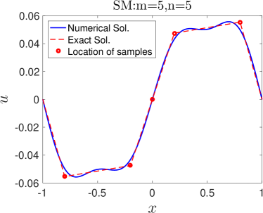
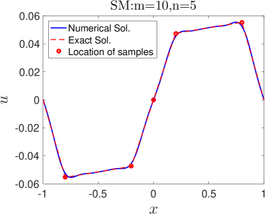
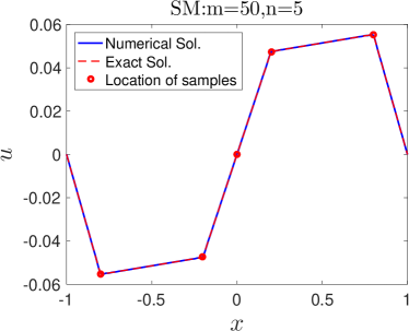
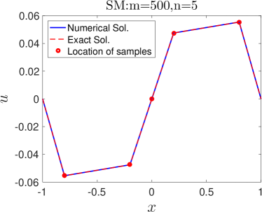
Figure 2: (Example 1): Numerical solutions in SM with 5 sampling points.

DNN method. For a better comparison with R-G method, we choose the activation function by $\sin(x)$ in DNN with one hidden layer. And the number of neurons are taken as $m=5,10,50,500$. The loss function (14) is selected with the parameter $\beta=10$. We reduce the loss to an order of 1e-4, and take learning rate by 1e-4. And 1000 test points are used to plot the figures. The DNN solutions are shown in Fig. 3, in which we observe that the DNN solutions are always smooth even when $m$ is very large.

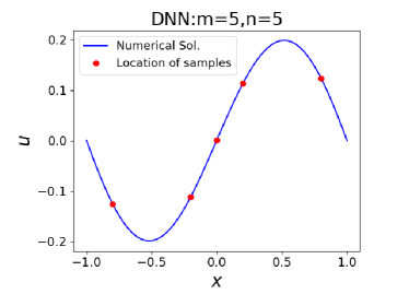
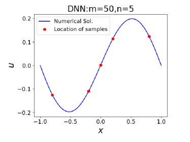
Figure 3: (Example 1): Numerical solutions in DNN method with 5 sampling points.

Example 2: In this example, we use the ReLU function as the basis function in R-G method and the activation function in DNN method to repeat the experiments in Example 1. Here we randomly choose another 10 sampling points.

Since the linear finite element function $\phi_{j}(x)$ can be expressed by ReLU functions for one dimensional case, namely,

$$\phi_{j}(x)=\frac{1}{h_{j-1}}\text{ReLU}(x-x_{j})-(\frac{1}{h_{j-1}}+\frac{1}{h_{j}})\text{ReLU}(x-x_{j})+\frac{1}{h_{j}}\text{ReLU}(x-x_{j+1}),$$

where $h_{j}=x_{j+1}-x_{j}$, we can use ReLU as the basis function for R-G method. For convenience, we just use the linear finite element function $\phi_{j}(x)$ instead of ReLU function as the basis function. Fig. 4 shows that there is no doubt that the FEM solution approximates the piecewise linear solution (27).

In DNN method, we choose the number of neurons $m=5,10,50,500$, respectively. And we use the variational from of the loss function (15) because of the second order derivative of ReLU function is always zero. Fig. 5 shows that the DNN learns the data as a relatively smoother function than the R-G method.

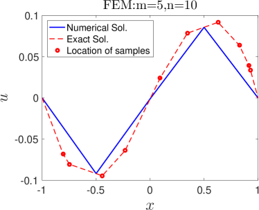
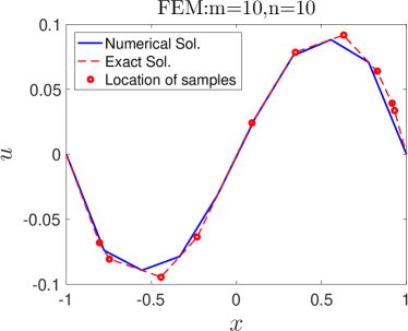
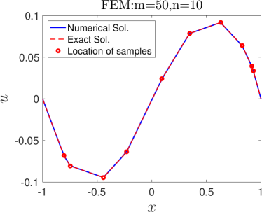
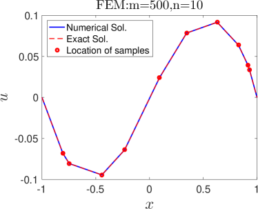
Figure 4: (Example 2): Numerical solutions in FEM with 10 sampling points.

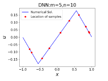
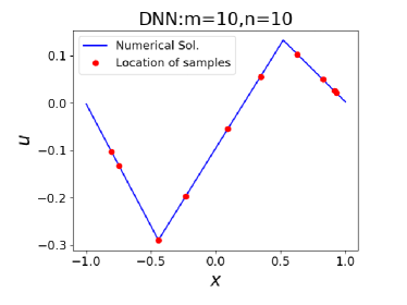
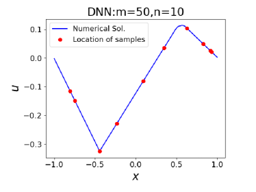
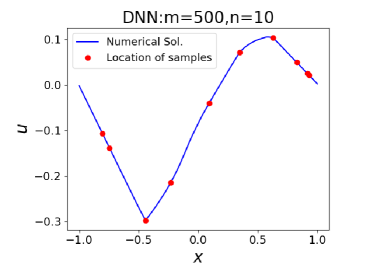
Figure 5: (Example 2): Numerical solutions in DNN method with ReLU activation function and 10 sampling points.

Example 3: We consider the 2D case

$$\left\{\begin{array}[]{c}-\Delta u(\bm{x})=f(\bm{x}),\quad\bm{x}\in(0,1)^{2},\\ u(\bm{x})=0,\quad\bm{x}\in\partial(0,1)^{2},\end{array}\right.$$

where $\bm{x}=(x,y)$ and we know the values of $f$ at $n$ points sampled from the function $f(\bm{x}):=f(x,y)=2\pi^{2}\sin(\pi x)\sin(\pi y).$ We fix the number of sample points $n=5^{2}$. The sampling points in the $x$ direction and the $y$ direction are both at $x_{h}=[0.1,0.25,0.5,0.8,0.9]$. We test the solution with the number of basis $m=5,50,100,200$, respectively. Fig. 6 plots the R-G solutions with Legendre basis and piecewise linear basis function. It can be seen that the numerical solution is a function with strong singularity. Fig. 7 shows the profile of R-G solutions at $y=0.5$ for various $m$, in which we can see that the values of numerical solutions at the sampling points get larger and larger with the increase of $m$. However, Fig. 8 shows that the DNN solutions are stable without singularity for large $m$.

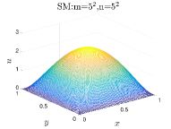
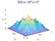
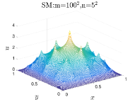
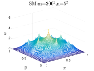
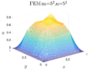
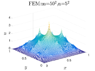
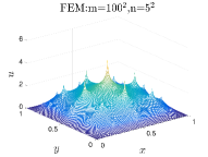
Figure 6: (Example 3): R-G solutions with different $m$. The basis functions for the first and the second row are Legendre basis function and piecewise linear basis function, respectively.

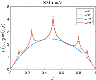
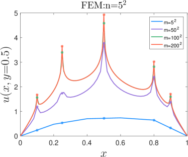
Figure 7: (Example 3): Profile of R-G solutions with different $m$.

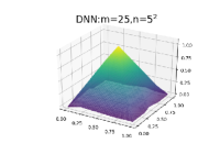
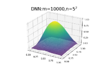
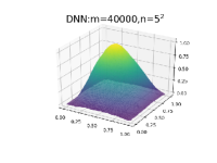
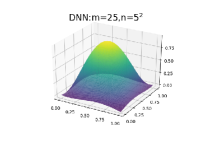
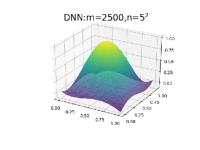
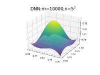
Figure 8: (Example 3): DNN solutions with different $m$. The activation functions for the first and the second row are ${\rm ReLU}(x)$ and $\sin(x)$, respectively.

4 Discussion of DNN method in solving PDE

DNNs are widely used in solving PDEs, especially for high-dimensional problems. The optimizing the loss functions in Eqs. (14) and (15) are equivalent to solving (8) except that the bases in (14) and (15) are adaptive. In addition, the DNN problem is optimized by (stochastic) gradient descent. The experiments in the previous section have shown that when the number of bases goes to infinity, DNN methods solve (3) by a relatively smooth and stable function compared with the one obtained by Theorem 1. We now utilize the F-Principle to understand what leads to the smoothness.

For two-layer wide DNNs with $d=1$, the two terms of $\Gamma(\bm{\xi})$ in the minimization problem of (20) yield different fitting results. Note that $\min\int_{R}||\bm{\xi}||^{-2}|\mathcal{F}[h](\bm{\xi})|^{2}\mathrm{d}\bm{\xi}$ leads to a piecewise linear function, while $\min\int_{R}||\bm{\xi}||^{-4}|\mathcal{F}[h](\bm{\xi})|^{2}\mathrm{d}\bm{\xi}$ leads to a cubic spline. Since the DNN is a combination of both terms, therefore, the DNN would yields to a much smoother function than the piecewise linear function. For a general DNN, the coefficient $\Gamma(\bm{\xi})$ in (19) cannot be obtained exactly, however, the monotonically decreasing property of $\Gamma(\bm{\xi})$ with respect to $\bm{\xi}$ can be postulated based on the F-Principle.

5 Conclusion

This paper compares the different behaviors of Ritz-Galerkin method and DNN method through solving PDEs to better understand the working principle of DNNs. We consider a particular Poisson problem (3), where the r.h.s. term $f$ is a discrete function. We analyze why the two numerical methods behave differently in theory. R-G method deals with the discrete $f$ as the linear combination of Dirac delta functions, while DNN methods implicitly bias towards functions with more low-frequency components to interpolate the discrete sampling points due to the F-Principle. Furthermore, from the numerical experiments, as the number of bases increases, one can see that the solutions obtained by R-G method approximate piecewise linear functions for 1d case and singular function for the 2d case, regardless of the basis function, but the solutions obtained by DNN method are smoother for 1d case and stable for the 2d case. In conclusion, based on the theoretical and numerical study in comparison to traditional methods in solving PDEs, DNN method possesses special implicit bias towards low frequencies, which leads to a well-bahaved solution even in a heavily over parameterized setting.

References

- [1] S. C. Brenner and L. R. Scott, The mathematical theory of finite element methods, Springer, New York, third edition, 2008.
- [2] W. Cai, X. G. Li and L. Z. Liu, A phase shift deep neural network for high frequency approximation and wave problems, SIAM J. Sci. Comput., 42(2020), A3285-A3312.
- [3] Z. Q. Cai, J. S. Chen, M. Liu and X. Y. Liu, Deep least-squares methods: an unsupervised learning-based numerical method for solving elliptic PDEs, J. Comput. Phys., 420(2020), 109707.
- [4] W. N. E, J. Q. Han and A. Jentzen, Deep learning-based numerical methods for high-dimensional parabolic partial differential equations and backward stochastic differential equations, Commun. Math. Stat., 5(2017), 349-380.
- [5] W. N. E and B. Yu, The deep ritz method: A deep learning-based numerical algorithm for solving variational problems, Commun. Math. Stat., 6(2018), 1-12.
- [6] A. Hamilton, T. Tran, M. Mckay, B. Quiring and P. Vassilevski, DNN approximation of nonlinear finite element equations, Tech. rep., Lawrence Livermore National Lab.(LLNL), Livermore, CA (United States), 2019.
- [7] J. Q. Han, A. Jentzen and E. Weinan, Solving high-dimensional partial differential equations using deep learning, P. Natl. Acad. Sci., 115(2018), 8505-8510.
- [8] J. C. He, L. Li, J. C. Xu and C. Y. Zheng, ReLU deep neural networks and linear finite elements, J. Comput. Math., 38(2020), 502-527.
- [9] Y. L. Liao and P. B. Ming, Deep Nitsche method: Deep Ritz method with essential boundary conditions, arXiv preprint arXiv:1912.01309, 2019.
- [10] Z. Q. Liu, W. Cai and Z. Q. J. Xu, Multi-scale deep neural network (mscaleDNN) for solving Poisson-Boltzmann equation in complex domains, Commun. Comput. Phys., to appear.
- [11] T. Luo, Z. Ma, Y. Y. Zhang and Z. Q. J. Xu, On the exact computation of linear frequency principle dynamics and its generalization, arXiv preprint arXiv:2010.08153, 2020.
- [12] A.D. Polyanin, Handbook of Linear Partial Differential Equations for Engineers and Scientists, Chapman & Hall/CRC, 2002.
- [13] C.P. Robert and G. Casella, Monte Carlo Statistical Methods, Springer, New York, 2004.
- [14] J. Shen, T. Tang and L. L. Wang, Spectral methods. Algorithms, analysis and applications, Springer, 2011.
- [15] J. W. Siegel and J. C. Xu, On the approximation properties of neural networks, arXiv preprint arXiv:1904.02311, 2019.
- [16] Z. J. Wang, Z. W. Zhang, A mesh-free method for interface problems using the deep learning approach, J. Comput. Phys., 400(2020), 108963.
- [17] Z. Q. J. Xu, Y. Y. Zhang, T. Luo, Y. Y. Xiao and Z. Ma, Frequency principle: Fourier analysis sheds light on deep neural networks, Commun. Comput. Phys., to appear.
- [18] Z. Q. J. Xu, Y. Y. Zhang and Y. Y. Xiao, Training behavior of deep neural network in frequency domain, International Conference on Neural Information Processing, 264-274, 2018.
- [19] Y. Y. Zhang, Z. Q. J. Xu, T. Luo and Z. Ma, Explicitizing an implicit bias of the frequency principle in two-layer neural networks, arXiv preprint arXiv:1905.10264, 2019.