Interpreting Interpretations: Organizing Attribution Methods by Criteria

Abstract

Motivated by distinct, though related, criteria, a growing number of attribution methods have been developed to interprete deep learning. While each relies on the interpretability of the concept of “importance“ and our ability to visualize patterns, explanations produced by the methods often differ. As a result, input attribution for vision models fail to provide any level of human understanding of model behaviour. In this work we expand the foundations of human-understandable concepts with which attributions can be interpreted beyond ”importance” and its visualization; we incorporate the logical concepts of necessity and sufficiency, and the concept of proportionality. We define metrics to represent these concepts as quantitative aspects of an attribution. This allows us to compare attributions produced by different methods and interpret them in novel ways: to what extent does this attribution (or this method) represent the necessity or sufficiency of the highlighted inputs, and to what extent is it proportional? We evaluate our measures on a collection of methods explaining convolutional neural networks (CNN) for image classification. We conclude that some attribution methods are more appropriate for interpretation in terms of necessity while others are in terms of sufficiency, while no method is always the most appropriate in terms of both.

1 Introduction

Among approaches for interpreting opaque models are input attribution which assign to each model input a level of contribution to its output. When visualized alongside inputs, an attribution gives a human interpreter some notion of what about the input is important to the outcome (see, for example, Figure 2). Being explanations of highly complex systems intended for highly complex humans, attributions have been varied in their approaches and sometimes produce distinct explanations for the same outputs.

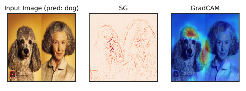
Figure 1: Interpreting the neural network prediction with different method may come with divergence. Left: the input with both predicted class and groundtruth being dog. Middle: SmoothGrad [23]. Pixels with deeper color have higher attribution scores. Right: GradCAM[19]. Regions with more heat localize the more relevant spatial locations. Questions: Is the model using the lady to classify the dog? Which interpretation is supposed to be used?

Nevertheless, save for the earliest approaches, attribution methods distinguish themselves with one or more desirable criteria. Scaling criteria such as completeness [25], sensitivity-n [2], linear-agreement [13, 25] calibrate attribution to the change in output as compared to change in input when evaluated on some baseline.Given access to different attribution methods, which one is the optimal choice for what purpose remains an unexplored area. Visual comparisons, though intuitive and straightforward, remains less objective since 1) humans’ ideas themselves do not accord at the most of time. 2) attribution maps generated by different methods may vary or even cause contradictory interpretations (see Fig 1 for example).

While evaluation criteria endow attributions with some limited semantics, the variations in design goals, evaluation metrics, and the underlying methods resulted in attributions failing at their primary goal: aiding in model interpretation. This work alleviates these problems and makes the following contributions.

• We decompose and organize existing attribution methods’ goals along two complementary properties: ordering and proportionality. While ordering requires that an attribution should order input features according to some notion of importance, proportionality stipulates also a quantitative relationship between a model’s outputs and the corresponding attributions in that particular ordering.

• We describe how all existing methods are motivated by an attribution ordering corresponding roughly to the logical notion of necessity which leads to a corresponding sufficiency ordering not yet fully discussed in literature.

• We show that while some attribution methods show great performance in necessity while others show more about sufficiency but no evaluated method in this paper can be a winner on the necessity and sufficiency at the same time.

• We further demonstrate how to interpret different attribution maps to gain more insights about the decision making process in deep models.

2 Background

Attributions are a simple form of model explanations that have found significant application to Convolutional Neural Networks (CNNs) with their ease of visualization alongside model inputs (i.e. images). We summarize the various approaches in Section 2.1 and the criteria with which they are evaluated and/or motivated in Section 2.3.

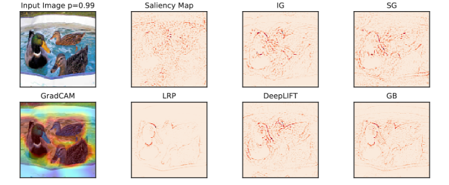
Figure 2: Visualizations of different attribution methods using VGG16 model [22]. (a) is the input image with an output confidence 0.99 for the true label ”duck”. (b)-(i): different attribution methods discussed in Section 2.1. grad $\times$ input is applied to (b), (c), (g), (h) and (i) to find attribution scores, while (d), (e) and (f) consider their results as attribution scores already. Use heatmap for (d) as the choice in [19].

2.1 Attribution Methods

The concept of Attribution is well-defined in [25] but it excludes any method without an baseline (reference) input. We consider a relaxed version. Consider a classification model $\mathbf{y}=M(\mathbf{x})$ that takes an input vector $\mathbf{x}$ and outputs a score vector $\mathbf{y}=[y_{0},\cdots,y_{i},\cdots,y_{n-1}]^{\top}$, where $y_{i}$ is the score of predicting $\mathbf{x}$ as class $i$ and there are $n$ classes in total. Given a pre-selected class $c$, an attribution method attempts to explain $y_{c}$ by computing a score for each feature $x_{i}$ as its contribution toward $y_{c}$. Even though each feature in $\mathbf{x}$ may receive different attribution scores given different choice of attribution methods, features with positive attribution scores are universally explained as important part in $\mathbf{x}$, while the negative scores indicate the presence of these features decline the confidence for predicting $y_{c}$.

Previous work has made great progress in developing gradient-based attribution methods to highlight important features in the input image for explaining model’s prediction. The primary question to answer is whether should we consider grad or grad $\times$ input as attributions [23, 25, 20, 14]. As Ancona et al. [2] argues grad is local attribution that only accounts for how tiny change around the input will influence the output of the network but grad $\times$ input is the global attribution that accounts for the marginal effect of a feature towards output. We use grad $\times$ input as the attribution to be discussed in this paper. We briefly introduce methods to be evaluated in this paper and examples are provided in Fig 2.

Saliency Map (SM) [21, 5] uses the gradient of the class of interests with respect to the input to interpret the prediction result of CNNs. Guided Backpropagation (GB) [24] modifies the backpropagation of ReLU [12] so that only the positive gradients will be passed into the previous layers. GradCAM [19] builds on the Class Activation Map (CAM) [27] targeting CNNs. Although its variations [7, 17] show sharper visualizations, their fundamental concepts remain unchanged. We consider only GradCAM in this paper. Layer-wise Relevance Propagation (LRP) [4], DeepLift [20] modifies the local gradient and rules of backpropagations. Another method sharing similar motivation in design with DeepLift is Integrated Gradient (IG) [25]. IG computes attribution by integrating the gradient over a path from a pre-defined baseline to the input. SmoothGrad (SG) [23] attempts to denoise the result of Saliency Map by adding Gaussian noise to the input and provides visually sharper results.

Other methods like Deep Taylor Decompostion [15] related with LRP, Occluding [26] and Influence Directed Explanations [13] are not evaluated in this paper but will be a proper future work to discuss.

2.2 Assumptions

We restrict ourselves with two assumptions with regards to models and attribution methods analyzed.

Non-linearity We focus on evaluating the performance of attribution methods on non-linear model, e.g. neural networks, as SM, IG, SG, LRP, and DeepLIFT are equivalent for linear models (see proofs in Appendix I) while GradCAM only works for convolutional layers. Linear models are therefore not expected to distinguish most attribution methods.

Feature Interaction Features may or may not influence the decision individually. In this paper, we focus on attribution methods that are not directly suited to reasoning about feature interaction: their attribution maps represent per-pixel importance, and do not indicate relationships between pixels. We are interested in evaluating the feature interactions in the future work.

2.3 Evaluation Criteria

Evaluation criteria measure the performance of attribution methods towards some desirable characteristic and are typically employed to justify the use of novel attribution methods. We begin with discussing two assumptions about evaluating the attribution methods.

The most common evaluations are based on pixel-level interventions or perturbations. These quantify the correlation between the perturbed pixels’ attribution scores and the output change [3, 6, 7, 11, 16, 18, 20]. For perturbations that intend to remove or ablate a pixel (typically by setting it to some baseline or to noise), the desired behavior for an optimal attribution method is to have perturbations on the highly attributed pixels drop the class score more significantly than on the pixels with lower attribution.

Quantification of the behavior described by Samek et al. [18] with Area Over Perturbation Curve (AOPC) measures the area between two curves: the model’s output score against the number of perturbed pixels in the input image and the horizontal line of the score at the model’s original output. Two similar measurement are Area Under Curve (AUC) [6, 16] and MOst Relevant features First (MoRF) [2] that measure the area under the perturbation curve instead. AOPC and AUC (we use AUC to represent both AUC and MoRF) measurement are equivalent and both are orignally used to endorse LRP. For reasons which will become clear in the next section, we categorize these criteria as supporting necessity order. We argue that evaluating attribution methods only with perturbation curves, e.g. Area Under Curve (or AUC), only discovers the tip of the iceberg and potentially can be problematic. A toy model is shown in Example 1 to elaborate our concerns.

Example 1.

Consider a model $M(\mathbf{x})=max(x_{1},x_{2})$ that takes a vector $\mathbf{x}$ with three features $x_{1},x_{2},x_{3}\in\{0,1\}$. Given the input to the model is $x_{1}=x_{2}=x_{3}=1$, assume $A_{1},A_{2},A_{3}$ are three different methods and output the attribution scores $s_{1},s_{2},s_{3}$ shown in Table 1 for each input feature $x_{1},x_{2},x_{3}$, respectively.

	$s_{1}$	$s_{2}$	$s_{3}$
$A_{1}$	$1/6$	$1/3$	$1/2$
$A_{2}$	$2/3$	$0$	$1/3$
$A_{3}$	$2/3$	$1/3$	$0$

Table 1: $s_{1},s_{2},s_{3}$ are attribution scores for $x_{1},x_{2},x_{3}$ computed by $A_{1},A_{2},A_{3}$, respectively.

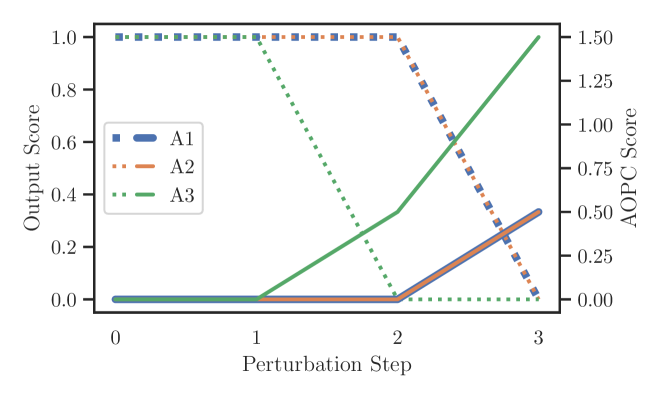
Figure 3: Comparing attribution methods $A_{1},A_{2}$ and $A_{3}$ by applying zero perturbation. Dash lines are the change of model’s output at each perturbation step (only one feature is set to 0 at each step). Solid lines are the changes of AOPC scores. $A_{2}$ and $A_{3}$ are overlapping with each other in this exmaple.

We apply zero perturbation to the input which means we set features to 0. The AOPC evaluation for these three attribution methods is shown in Fig 3. Using the conclusion from [18] that higher AOPC scores suggest higher relativity of input features highlighted by an attribution method, Fig 3 shows pixels highlighted by $A_{3}$ are more relative Samek et al. [18] to prediction than $A_{1}$ and $A_{2}$, as expected. However, $A_{2}$ and $A_{1}$ are considered as showing same level of relativity under the AOPC measurement even though $A_{2}$ succeeds in discovering $a$ is more relevant than $c$, whereas $A_{1}$ believes $c$ is more relevant than both $a,b$.

Another set of criteria instead stipulate that positively attributed features should stand on their own independently of non-important features. An example of this criterion is Average % Drop [7] in support of GradCam++ that measures the change of class score by presenting only pixels highlighted by an attribution only (non-important pixels are ablated). Another example is the LEast Relevant Features first (LeRF) [2] that removes the features with least high attribution scores. first. We will say these two criteria support sufficiency order (definition to follow).

Rethinking the concept of relativity, we believe both necessity and sufficiency can be treated as different types of relativity. In Example 1, neither $x_{1}$ nor $x_{2}$ is a necessary feature individually because the output will not change if any one of them is absent. However, both $x_{1}$ and $x_{2}$ are sufficient features, with either of which, the model could produce the same output as before. Besides, $A_{2}$ succeeds in placing the order of sufficient feature $x_{1}$ in front of the non-sufficient feature $x_{3}$ but $A_{2}$ fails, while AOPC(or AUC) is unable to discover the success.

Other evaluation criteria exist, like sensitivity-n [2] and sanity check [1], will be discussed in Section 5.

3 Methods

To tame the zoo of criteria, we organize and decompose them into two aspects: (1) ordering imposes conditions under which an input should be more important than another input in a particular prediction, and (2) proportionality further specifies how attribution should be distributed among the inputs. We elaborate on ordering criteria in Section 3.2 with instantiating in Section 3.3 and Section 3.4. We describe proportionality in Section 3.5. We begin with the logical notions of necessity and sufficiency as idealized versions of ablation-based measures described in Section 2. We introduce our notations in this paper before any further discussion,

3.1 Notation

Consider a model $y=f(\mathbf{x})$ and an attribution method $A$, it computes a set of attribution scores $s_{1},s_{2},...,s_{n}$ for each pixel $x_{1},x_{2},...,x_{n}$ in the input image $\mathbf{x}$ attributing a given class . We permute the pixels into a new ordering $\pi_{A}(\mathbf{x})=[x^{\prime}_{1},x^{\prime}_{2},...,x^{\prime}_{n}]$ so that $s^{\prime}_{1}\geq s^{\prime}_{2}\geq...\geq s^{\prime}_{n}$. We take the subset $\pi^{+}_{A}(\mathbf{x})$ of $\pi_{A}(\mathbf{x})$ so that $\pi^{+}_{A}(\mathbf{x})$ has the same ordering as $\pi_{A}(\mathbf{x})$ but only contains pixels with positive attribution scores. Let $R_{i}(\mathbf{x},\pi)$ be the output of the model with input $\mathbf{x}$ where pixels $x^{\prime}_{1},x^{\prime}_{2},...,x^{\prime}_{i}\in\pi$ are perturbed from the input by setting $x^{\prime}_{1}=x^{\prime}_{2}=...=x^{\prime}_{i}=b$, where $b$ is a baseline value for the image (typically $b=0$). Also, let $\mathbf{x}_{b}$ be the the baseline input image where all the pixels are filled with the baseline value $b$. Therefore, we have the the original output $y_{0}=f(\mathbf{x})$ and the baseline output $y_{b}=f(\mathbf{x}_{b})$.

3.2 Logical Order

The notions of necessity and sufficiency are commonly used characterizations of logical conditions. A necessary condition is one without which some statement does not hold. For example, in the statement $P_{1}=A\wedge B$, both $A$ and $B$ are necessary conditions as each independently would invalidate the statement were they be made false. On the other hand, a sufficient condition is one which can independently make a statement true without other conditions being true. In more complex statements, no atomic condition may be necessary nor sufficient though compound conditions may. In the statement $P_{3}=(A\wedge B)\vee(C\wedge D)$, none of $A,B,C,D$ are necessary nor sufficient but $(A\wedge B)$ and $(C\wedge D)$ are sufficient. As we are working in the context of input attributions, we relax and order the concept of necessity and sufficiency for atomic conditions (individual input pixels).

Definition 1 (Logical Necessity Ordering).

Given a statement $P$ over some set of atomic conditions, and two orderings $a$ and $b$, both ordered sets of the conditions, we say $a$ has better necessity ordering for $P$ than $b$ if:

$$\min_{i}\left(\left\{a_{k}\right\}_{k\geq i}\cancel{\models}P\right)\leq\min_{i}\left(\left\{b_{k}\right\}_{k\geq i}\cancel{\models}P\right)$$ (1)

Definition 2 (Logical Sufficiency Ordering).

Likewise, $a$ has better sufficiency ordering for $P$ than $b$ if:

$$\min_{i}\left(\left\{a_{k}\right\}_{k\leq i}\models P\right)\leq\min_{i}\left(\left\{b_{k}\right\}_{k\leq i}\models P\right)$$ (2)

A better necessity ordering is one that invalidates a statement $P$ by removing the shorter prefix of the ordered conditions while a better sufficiency ordering is the one that can validate a statement using the shorter prefix.

3.3 Necessity Ordering (N-Ord)

Unlike logical statements, numeric models do not have an exact notion of a condition (feature) being present or not. Instead, inputs at some baseline value or noise are viewed as having a feature removed from an input. Though this is an imperfect analogy, the approach is taken by every one of the measures described in Section 2 that make use of perturbation in their motivation. Additionally, with numeric outputs, the nuances in output obtain magnitude and we can longer describe an attribution by a single index like the minimal index of Definitions 1 and 2. Instead we consider an ideal ordering as one which drops the numeric output of the model the most with the least number of inputs ablated.

We refer the AUC measurement [6, 16] and MoRF [2] as means to measure the Necessity Ordering (N-Ord). Denote $N_{o}(\mathbf{x},A)$ as N-Ord score given a input image $\mathbf{x}$ and an attribution method $A$. Rewrite AUC using the notation in Section 3.1:

$$N_{o}(\mathbf{x},A)=\frac{1}{M+1}\sum^{M}_{m=0}R^{m}_{0}(\mathbf{x},A)$$ (3)

where $R^{m}_{0}(\mathbf{x},A)=max\{R_{m}(\mathbf{x},\pi^{+}_{A}(\mathbf{x}))-y_{b},0\}$ and $M$ is the total number of pixels in $\pi^{+}_{A}(X)$. We include $max$ to clip scores below the baseline output. According to Definition 1, we have the following proposition.

Proposition 1.

An attribution method $A_{1}$ shows a (strictly) better Ordering Necessity than another method $A_{2}$ given an input image $\mathbf{x}$ if $N_{o}(\mathbf{x},A_{1})<N_{o}(\mathbf{x},A_{2})$

As discussed in Section 2.3, N-Ord only captures whether more necessary pixels, are receiving higher attribution scores. We argue that attribution methods should also be differentiated by the ability of highlighting sufficient features. To evaluate whether more sufficient pixels are receiving higher attribution scores, we propose Sufficiency Ordering as a complementary measurement.

3.4 Sufficiency Ordering (S-Ord)

We believe LeRF [2] is a related means of measuring the Sufficiency. Sufficiency Ordering measures the score increase as we keep adding important features into a baseline input. Use the notation in Section 3.1 and let $R^{\prime}_{i}(\mathbf{x}_{b},\pi)$ be the model’s output with $\mathbf{x}_{b}$ where $x^{\prime}_{1},x^{\prime}_{2},\cdots,x^{\prime}_{i}\in\pi$ are added to the baseline image $\mathbf{x}_{b}$. Denote $S_{o}(\mathbf{x},A)$ as S-Ord score given a input image $\mathbf{x}$ and an attribution method $A$.

$$S_{o}(\mathbf{x},A)=\frac{1}{M+1}\sum^{M}_{m=0}R^{m^{\prime}}_{0}(\mathbf{x},A)$$ (4)

where $R^{m^{\prime}}_{0}(\mathbf{x},A)=min\{R^{\prime}_{m}(\mathbf{x}_{b},A),R^{\prime}_{M}(\mathbf{x}_{b},\pi^{+}_{A}(\mathbf{x}))\}-y_{0}$, $M$ is the number of pixels in $\pi^{+}_{A}(\mathbf{x})$. We include $min$ to clip scores above the original output. According to Definition 2, we have the following proposition.

Proposition 2.

An attribution method $A_{1}$ shows (strictly) better Ordering Sufficiency than another method $A_{2}$ given an input image $X$ if $S_{o}(\mathbf{x},A_{1})>S_{o}(\mathbf{x},A_{2})$.

N-Ord and S-Ord together provides a more comprehensive evaluation for an attribution method. In Section 3.5, we are going to discuss the disadvantages of only using N-Ord or S-Ord and propose Proportionality as a refinement to the ordering analysis.

3.5 Proportionality

N-Ord and S-Ord do not incorporate the attribution scores beyond producing an ordering. This can be an issue toward an accurate description of feature necessity or sufficiency. For example, consider a toy model $M(x_{1},x_{2})=2x_{1}+x_{2}$ and let the inputs variables be $x_{1}=x_{2}=1$. Any attribution methods that assign higher score for $x_{1}$ than $x_{2}$ produces the identical ordering $\pi(x_{1},x_{2})=[x_{1},x_{2}]$, even one could overestimate the degree of necessity (or sufficiency) of $x_{1}$ by assigning it with much higher attribution scores. With linear agreement [14], scores for $x_{1}$ and $x_{2}$ are more reasonable if their ratio is close to 2:1. Explaining a decision made by a more complex model only using ordering of attributions may overestimate or underestimate the necessity (or sufficiency) of an input feature. Therefore, We propose Proportionality as a refinement to quantify the necessity and sufficiency in complementary to the ordering measurement.

Definition 3 (Proportionality-k for Necessity).

Consider two positive number $n_{1},n_{2}$ and an attribution method A. Use notations in Section 3.1 and let $\hat{\pi}^{+}_{A}(\mathbf{x})$ be a reversed ordering of $\pi^{+}_{A}(\mathbf{x})$. Proportionality-k for Necessity is measured by

$$N^{k}_{p}(\mathbf{x},A)=|R_{n_{1}}(\mathbf{x},\pi^{+}_{A}(\mathbf{x}))-R_{n_{2}}(\mathbf{x},\hat{\pi}^{+}_{A}(\mathbf{x}))|$$ (5)

under the condition $\sum^{n_{1}}_{i}s_{i}=\sum^{n_{2}}_{j}s_{j}=kS(A,\mathbf{x}),s_{i}\in\pi^{+}_{A}(\mathbf{x}),s_{j}\in\hat{\pi}^{+}_{A}(\mathbf{x}),k\in[0,1]$. $R_{i}(\mathbf{x},\pi)$ uses the same definition in (3), and $S(\mathbf{x},A)$ is the sum of total positive attribution scores.

Explanation of Definition 3 the motivation behind Proportionality-k for Necessity is that: given a group of pixels ordered with their attribution scores, there are different ways of distributing scores to each feature while the ordering remains unchanged. An optimal assignment is preferred that features receive attribution scores proportional to the output change if they are modified accordingly. In other words, given any two subsets of pixels $\pi_{1}$ and $\pi_{2}$. with total attribution scores sum to $S_{1}$ and $S_{2}$, are perturbed, the change of output scores $R(\mathbf{x},\pi_{1})$ and $R(\mathbf{x},\pi_{2})$ should satisfy $R(\mathbf{x},\pi_{1})/R(\mathbf{x},\pi_{2})=S_{1}/S_{2}$. This property is demanded because the same share of attribution scores should account for the same necessity or sufficiency. If we restrict the condition to $S_{1}=S_{2}$, the difference between $R(\mathbf{x},\pi_{1})$ and $R(\mathbf{x},\pi_{2})$ becomes an indirect measurement of the proportionality. For the measurement of Necessity, we further restrict that $\pi_{1}$ is perturbed from the pixel with the highest attribution score first and $\pi_{2}$ is perturbed from the one with lowest attribution score first, in accordance with the setup in N-Ord. Therefore, a smaller difference $N^{k}_{p}(\mathbf{x},A)$ shows better Proportionality-k for Necessity

Proposition 3.

An attribution method $A_{1}$ shows better Proportionality-k for Necessity than method $A_{2}$ if $N^{k}_{p}(\mathbf{x},A_{1})<N^{k}_{p}(\mathbf{x},A_{2})$

A similar requirement for attribution method is completeness discussed by [25] and its generalization sensitivity-n discussed by [2]. completeness requires the sum of total attribution scores to be equal to the change of output compared to a baseline input, and sensitivity-n requires any subset of $n$ pixels whose summation of attribution scores should be equal to the change of output compared to the baseline if pixels in that subset are removed. When $n$ is the total number of pixels in the input image, sensitivity-n reduces to completeness. The relationships between sensitivity-n and Proportionality-k for Necessity are discussed as follows:

Proposition 4.

If an attribution method $A$ satisfies both sensitivity-$n_{1}$ and sensitivity-$n_{2}$, then $N^{k}_{p}(\mathbf{x},A)=0$ under the condition if $\sum^{n_{1}}_{i}s_{i}=\sum^{n_{2}}_{j}s_{j}=kS(\mathbf{x},A),s_{i}\in\pi^{+}_{A}(\mathbf{x}),s_{j}\in\hat{\pi}^{+}_{A}(\mathbf{x}),k\in[0,1]$ , but not vice versa.

The proof for Proposition Appendix I: Proofs and can be found in Appendix 1. We further contrast our method with sensitivity-n in Section 5. Integrating proportionality with all possible shares of attribution scores, we define the Total Proportionality for Necessity (TPN):

Definition 4 (Total Proportionality for Necessity).

Given an attribution method A and an input image $\mathbf{x}$, The Total Proportionality for Necessity is measured by

$$N_{p}(\mathbf{x},A)=\frac{1}{ry_{0}}\int^{1}_{0}N^{k}_{p}(\mathbf{x},A)dk$$ (6)

where $r=\min\{y_{b}/R_{M}(\mathbf{x},\pi^{+}_{A}(\mathbf{x})),1\}$. $y_{0}$ is used as a normalizer and $M$ is the total number of elements in $\pi^{+}_{A}(\mathbf{x})$, therefore, $r=1$ if removing all elements in $\pi^{+}_{A}(\mathbf{x})$ drops the score to the baseline. Revisit the Section 3.1 for notations if needed.

Explanation for Definition 4 $N_{p}(\mathbf{x},A)$ is the area between two perturbation curves one starting from the pixels with highest attribution scores and the other with a reversed ordering. The difference from Necessity Ordering is that $N_{p}(\mathbf{x},A)$ is measured against the share of attribution scores (the value of $k$) instead of the share of pixels in the $N_{o}(\mathbf{x},A)$. On the other side, perturbations on non-necessary features may not change the output at all and we penalize an attribution method that guides us to do so with the ratio $r$ compared to the baseline. Generalizing Proposition 3, we argue:

Proposition 5.

An attribution method $A_{1}$ shows better Total Proportionality for Necessity than method $A_{2}$ if $N_{p}(\mathbf{x},A_{1})<N_{p}(\mathbf{x},A_{2})$

Under the similar construction, we have the following definition of Proportionality-k for Sufficiency and Total Proportionality for Sufficiency (TPS):

Definition 5 (Proportionality-k for Sufficiency).

Consider two positive number $n_{1},n_{2}$ and an attribution method A. Use notations in Section 3.1 and let $\hat{\pi}^{+}_{A}(\mathbf{x})$ be a reversed ordering of $\pi^{+}_{A}(\mathbf{x})$. Proportionality-k for Sufficiency is measured by

$$S^{k}_{p}(\mathbf{x},A)=|R^{\prime}_{n_{1}}(\mathbf{x}_{b},\pi^{+}_{A}\mathbf{x}))-R^{\prime}_{n_{2}}(\mathbf{x}_{b},\hat{\pi}^{+}_{A}(\mathbf{x}))|$$ (7)

under the condition $\sum^{n_{1}}_{i}s_{i}=\sum^{n_{2}}_{j}s_{j}=kS(\mathbf{x},A),s_{i}\in\pi^{+}_{A}(\mathbf{x}),s_{j}\in\hat{\pi}^{+}_{A}(\mathbf{x}),k\in[0,1]$. $R^{\prime}_{i}(\mathbf{x},\pi)$ reuses the definition in (4); $S(\mathbf{x},A)$ is the sum of total positive attribution scores.

We want the difference $S^{k}_{p}(\mathbf{x},A)$ as small as possible since the same share of attribution scores should reflect same sufficiency. Therefore, we have the following proposition:

Proposition 6.

An attribution method $A_{1}$ shows better Proportionality-k for Sufficiency than method $A_{2}$ if $S^{k}_{p}(\mathbf{x},A_{1})<S^{k}_{p}(\mathbf{x},A_{2})$

Definition 6 (Total Proportionality for Sufficiency).

Given an attribution method A and an input image $\mathbf{x}$, The Total Proportionality for Sufficiency is measured by

$$S_{p}(\mathbf{x},A)=\frac{1}{r^{\prime}y_{0}}\int^{1}_{0}S^{k}_{p}(\mathbf{x},A)dk$$ (8)

where where $r^{\prime}=\min\{R^{\prime}_{M}(\mathbf{x},\pi^{+}_{A}(\mathbf{x}))/y_{0},1\}$. $y_{0}$ is used as a normalizer and $M$ is the total number of elements in $\pi^{+}_{A}(\mathbf{x})$, therefore, $r^{\prime}=1$ if adding all elements in $\pi^{+}_{A}(\mathbf{x})$ increases the score to the original output. Refer to Section 3.1 and 3.4 for details about the notation.

Similarly, $S_{p}(\mathbf{x},A)$ is the area between curves of model’s output change by adding pixels to a baseline input with the highest attribution scores first or by the lowest first. The ratio $r^{\prime}$ penalizes the false postive situation when adding all pixels with positive scores does not increase the output significantly. Finally, we have

Proposition 7.

An attribution method $A_{1}$ shows better Total Proportionality for Sufficiency than another method $A_{2}$ if $S_{p}(\mathbf{x},A_{1})<S_{p}(\mathbf{x},A_{2})$

In summary, we differentiate and describe the Necessity Ordering (N-Ord) and Sufficiency Ordering (S-Ord) from previous work and propose Total Proportionality for Necessity (TPN) and Total Proportionality for Sufficiency (TPS) as refined evaluation criteria for necessity and sufficiency. We then apply our measurement to explain the prediction results from an image classification task in the rest of the paper.

4 Evaluation

4.1 Implementation of Proportionality

To compute TPN for each single input, we ablate a subset of input features at each time. Different from Ordering test, we do not ablate a certain number of features, instead, we ablate a subset of features with a certain share of attribution scores. The share of attribution scores $k$ goes from 0 to 1. We generate the ablation curve from the features with highest scores first and the features with least highest scores first, and measure the area between these two curves. Optimal TPN will be 0 as discussed in the previous sections. The similar implementation will be applid to TPS.

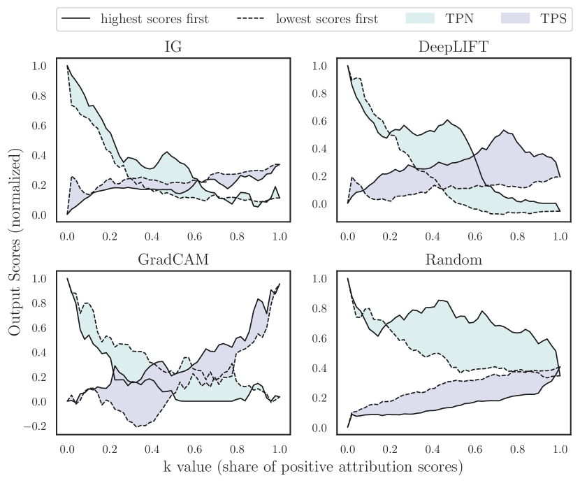
Figure 4: An example of computation for TPN and TPS with the input in Fig 2. The area represents the score of TPN and TPS before applying the penalty $r$ and $r^{\prime}$ for better visulization purpose. We also include a Random method that randomly assigns attribution scores first as a baseline method to compare with . This figure is better viewed in color.

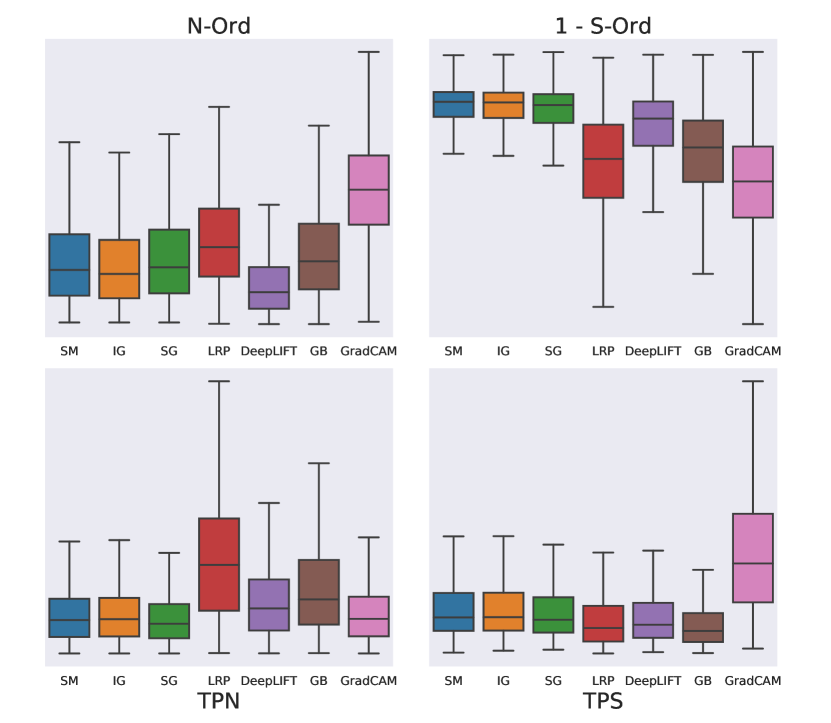
Figure 5: The boxplot for different attribution methods evaluated with four crietria aforementioned on 9600 images from ImageNet with VGG16 model. Since only the higher S-Ord score indicates better Sufficiency Ordering, we use $1-$ S-Ord to accord with other criteria so the lower scores will indicate better performance on all criteria shown above.

4.2 Evaluate on the datasets

We evaluate N-Ord, S-Ord, TPN and TPS on 9600 images sampled from ImageNet [10] on VGG16 models. We evaluate all the attribution methods motioned in Section 3 and the implementation detail for the model and attribution methods can be found in the Appendix 3. We show the boxplot in Fig 5. We plot $1-$ S-Ord instead the original S-Ord score so that that conclusion that lower scores represent better performance holds for all subfigures. On the ImageNet and VGG model, DeepLIFT has shown relatively better Necessity Ordering while GradCAM shows relatively better Sufficiency Ordering. Considering the proportionality, Saliency Map, Integrated Gradient and Smooth Gradient are all showing slightly better proportionality for necessity while LRP and GB are showing slightly better proportionality for sufficiency. But clearly, no evaluated method is significantly better than others on all criteria at the same time.

We analyze these attribution methods based on the result of Fig 5: Saliency Map performs not bad in necessity for both ordering and proportionality compared to sufficiency. Therefore, the features with highest scores assigned by Saliency Map may not be actually sufficient for the decision making process, e.g. the pool is highlighted by Sailency Map in Fig 2 but the model will probably not make a mistake when only the pool is present to it. One possible reason is that the vanishing gradient issue causes the loss of gradient signal. Threfore, Integrated Gradient and DeepLIFT are two means trying to solve the vanishing gradient issue in Saliency Map and both archive better Necessity Ordering compared to the Saliency Map. But they do not show significantly better proportionality in both necessity and sufficiency. The reason behind this we assume is that the Summation-to-Delta requirement only guarantees that sum of attribution scores for all features equals to the change of output, while any other share of attribution scores does not cause equivalent change to the output, so the proportionality is not improved. Similar conclusions are also discussed by sensitivity-n [2] Smooth Gradient shows lower inter-quartile range in both TPN and TPS compared to Saliency Map. Computing the expectation of the Saliency Map of a distribution of inputs does not resolve the possible vanishing gradients issue for each input in the distribution; however, at the same activation unit, e.g. ReLU, an input’s gradient signal is blocked by flatten negative region but its neighbor’s gradient signal can get unblocked. It may help to explain the improvement Smooth Gradient shows in th experiment. GradCAM is probably the best choices one can have for the Sufficiency Ordering regardless of the fact it does poorly in porportionality for the sufficiency – the attribution scores may not reflect actual sufficiency. The result is not surprising because the upsampling process in GradCAM does not relate to any axiom that guarantees to produce pixel-level proportional scores.

On the contradictory, we can not make instructive comment on the following two attribution methods: Guided Backpropagation shows better sufficiency on ordering and proportionality compared to the necessity. We consider it as a good method to reveal the sufficient features, however, as Adebayo et al. [1] points out GB lacks fearfulness to the model by behaving poorly in the sanity check. Therefore, we leave the understanding of GB as a future work. On the other hand, Layer-wise Relevance Propagation is the one we will not make much strong conclusion as well since there are many rules in LRP and only one of them, $\alpha 2\beta 1$-LRP (see Appendix II), is tested. But specifically, for $\alpha 2\beta 1$-LRP, it shows good sufficiency on both criteria, which increase our confidence to interpret the result of $\alpha 2\beta 1$-LRP as identifying sufficient features in the input space.

4.3 Evaluate with one instance

All the metrics discussed before can be applied to one single input and the interpretation using all winners for each criteria can provide more insights about the model. For example, in Fig 6, we interpret that the body of a dog is necessary to the English springer class and only providing the body the model may not consider it is a dog, the sufficient feature is its head. Consulting different attributions and interpret with the winners can give more comprehensive understandings. More exmaples are included in Appendix III.

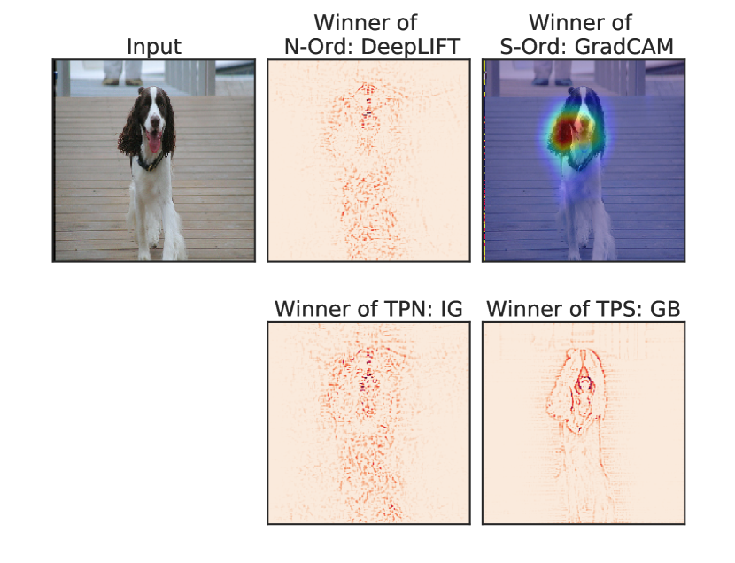
Figure 6: An example of interpreting the model’s predictions with winners on different criteria.

5 Related Work

To the best of our knowledge, we are the first one describing the concepts of necessity and sufficiency in attributions where similar work may only touch the surface of either necessity or sufficiency but not both. Our work is partially motivated by smallest sufficient region (SSR) and smallest destroying region (SDR) [8] where the authors aim to propose a region that either increase or decrease the model’s output most even though SSR and SDR only capture the spatial location in the image but do not incorporate the feature contributions as scores.

We also consider our work as a subset of sensitivity evaluation that how well we can trust an attribution method with its quantification of the feature importance in the input. A close concept is quantitative input influence by Datta et al. [9] (even though the author does not target on deep neural networks). sensitivity (a)(b) [25] provides the basis of discussion and sensitivity-n [2] imposes more strict requirements. The mathematical connection between proportionality with sensitivity-n is discussed in Section 3.5. We discuss the main difference of these two concepts here. proportionality approaches the sensitivity from a view that, regardless of the number of pixels, same share of attribution scores should account for same change to the output, while sensitivity-n requires removing $n$ pixels should change the output by the amount of total attribution scores of that $n$ pixels. sensitivity-n only provides True/False to an attribution methods, but proportionality provides numerical results for comparing different methods under two purposes, the necessity and sufficiency.

6 Conclusion

In this work, we summarized existing evaluation metrics for attribution methods and categorized them into two logical concepts, necessity and sufficiency. We then demonstrated realizable criteria to quantify necessity and sufficiency with an analysis focused on ordering and its refinement, proportionality. We evaluated existing attribution methods against our criteria and listed the best methods for each criteria. We discovered that certain attribution methods excel in necessity or sufficiency, but none is a frequent winner for both.

The logical concepts of necessity and sufficiency are generally mutually exclusive and our analogues show the same based on our results: no method is universally optimal for both necessity and sufficiency. While this means we cannot endorse one method over others, the techniques we present provide additional interpretability tools to data scientist who can use our measures to select the attribution appropriate to the task at hand. When debugging a model for identifying traffic stop signs, an analyst can select for methods with greater necessity to determine whether the model has learned spurious correlates, e.g., the pole holding up the sign. A “necessary” pole would lead to false negatives (stop signs not on poles) while a “sufficient” one would only indicate potential false positives (poles without stop signs) which, though also problematic, are not as dangerous as false negatives in this case. The increased basis with which to interpret attribution will hopefully lead to a fuller understanding of model behaviour.

Appendix

Appendix I: Proofs

Nonlinearity Ancona et al. [2] concludes that SM, IG, LRP,DeepLIFT are equivalent for linear models and their proof also applies to SG. We first introduce the following proposition:

Proposition 8.

All attribution methods mentioned in Sec 2 except GradCAM and Guided Backpropagation are equivalent if the model behaves linearly.

Proof.

As the Proposition 4 and Conclusion 6 in Ancona et al. [2] prove that Saliency Map, Integrated Gradient, DeepLIFT and LRP are equivalent for a linear model, we just need to prove SmoothGrad is equivalent to Saliency Map if the model is linear.

If a model behaves linearly, we can express the output score $y_{c}$ for class $c$ as a linear combination such that $y_{c}=\mathbf{w}^{\top}_{c}\mathbf{x}+b_{c}$. Then the SmoothGrad $S(\mathbf{x})_{c}$ is

$$S(\mathbf{x})_{c} =\mathbb{E}_{\boldsymbol{\epsilon}\sim\mathcal{N}(\mathbf{0},\mathbf{I}\lambda)}\frac{\partial[\mathbf{w}^{\top}_{c}(\mathbf{x}+\boldsymbol{\epsilon})+b_{c}]}{\partial\mathbf{x}}$$ (9)

$$=\mathbb{E}_{\boldsymbol{\epsilon}\sim\mathcal{N}(\mathbf{0},\mathbf{I}\lambda)}\mathbf{w}_{c}$$

$$=\mathbf{w}_{c}=\frac{\partial y_{c}}{\partial\mathbf{x}}\quad(\text{Saliency Map})$$

∎

Proof to Proposition 4 If an attribution method $A$ satisfies both sensitivity-$n_{1}$ and sensitivity-$n_{2}$, then $N^{k}_{p}(\mathbf{x},A)=0$ under the condition if $\sum^{n_{1}}_{i}s_{i}=\sum^{n_{2}}_{j}s_{j}=kS(\mathbf{x},A),s_{i}\in\pi^{+}_{A}(\mathbf{x}),s_{j}\in\hat{\pi}^{+}_{A}(\mathbf{x}),k\in[0,1]$ , but not vice versa.

Proof.

If A satisfies sensitivity-$n_{1}$, for any given ordered subset $\pi$, we have

$$\sum^{n_{1}}s_{i}=R(\mathbf{x},\pi)$$

Same thing happens to $n_{2}$ if A satisfies sensitivity-$n_{2}$. Under the condition if $\sum^{n_{1}}_{i}s_{i}=\sum^{n_{2}}_{j}s_{j}=kS(\mathbf{x},A),s_{i}\in\pi^{+}_{A}(\mathbf{x}),s_{j}\in\hat{\pi}^{+}_{A}(\mathbf{x}),k\in[0,1]$,

$$N^{k}_{p}(\mathbf{x},A) =|R(\mathbf{x},\pi_{A}(\mathbf{x})-R(\mathbf{x},\pi^{+}_{A}(\mathbf{x})|$$ (10)

$$=|\sum^{n_{1}}_{i}s_{i}-\sum^{n_{2}}_{j}s_{j}|$$

$$=|kS(\mathbf{x},A)-kS(\mathbf{x},A)|=0$$

∎

Appendix II: Implementation Details

Models

We evaluate N_Ord, S_Ord for all attribution methods mentioned in Section 2. We evaluate on 9600 images from ImageNet [10] with pre-trained on VGG16[22].

Attribution Methods

Saliency Map

As discussed in Sec 2, we use grad $\times$ input to represent the Saliency Map, instead of the vanilla gradient.

Integrated Gradient

We use the black image as the baseline for all images and we use the 50 samples on the linear path from the baseline to the input.

Smooth Gradient

As discussed in Sec 2, we use smooth_grad $\times$ input to represent the Smooth Gradient. We pick a noise level of 20 $\%$ as it appears to be the best parameter in its original paper [23]. We randomly sample 50 points from the Gaussian distribution for the aggregation.

DeepLIFT

We use the black image as the baseline for all images and we use the RevealCancel rule for DeepLIFT

LRP

We use the implementation of LRP-$\alpha 2\beta 1$ with generalization tricks mentioned by Montavon et al. [16] who argues this rule is better for image explanations.

Guided Backpropagation

To implement Guided Backpropagation, we modify the ReLU activation in the network to filter out the negative gradient in tensorflow.

⬇

@ops.RegisterGradient("GuidedBackProp")

def _GuidedBackProp(op, grad):

dtype = op.inputs[0].dtype

return grad * tf.cast(grad > 0., dtype) * \

tf.cast(op.inputs[0] > 0., dtype)

GradCAM

We use the last convolutional layer to compute the GradCAM for all images.

Appendix III

More examples of evaluating each images with TPN and TPS are shown in Fig 7

Figure 7: More visualizations of different attribution methods. Red checks mark the winner of Total Proportionality for Necessity and blue checks mark the winner of Total Proportionality for Sufficiency

References

- Adebayo et al. [2018] Julius Adebayo, Justin Gilmer, Michael Muelly, Ian Goodfellow, Moritz Hardt, and Been Kim. Sanity checks for saliency maps, 2018.
- Ancona et al. [2017] Marco Ancona, Enea Ceolini, Cengiz Öztireli, and Markus Gross. Towards better understanding of gradient-based attribution methods for deep neural networks, 2017.
- Ancona et al. [2017] Marco Ancona, Enea Ceolini, Cengiz Öztireli, and Markus Gross. A unified view of gradient-based attribution methods for deep neural networks. 11 2017).
- Bach et al. [2015] Sebastian Bach, Alexander Binder, Grégoire Montavon, Frederick Klauschen, Klaus-Robert Müller, Wojciech Samek, and Oscar Déniz Suárez. On pixel-wise explanations for non-linear classifier decisions by layer-wise relevance propagation. In PloS one, 2015).
- Baehrens et al. [2009] David Baehrens, Timon Schroeter, Stefan Harmeling, Motoaki Kawanabe, Katja Hansen, and Klaus-Robert Mueller. How to explain individual classification decisions, 2009.
- Binder et al. [2016] Alexander Binder, Grégoire Montavon, Sebastian Bach, Klaus-Robert Müller, and Wojciech Samek. Layer-wise relevance propagation for neural networks with local renormalization layers, 2016.
- Chattopadhay et al. [2018] Aditya Chattopadhay, Anirban Sarkar, Prantik Howlader, and Vineeth N Balasubramanian. Grad-cam++: Generalized gradient-based visual explanations for deep convolutional networks. 2018 IEEE Winter Conference on Applications of Computer Vision (WACV), Mar 2018).
- Dabkowski and Gal [2017] Piotr Dabkowski and Yarin Gal. Real time image saliency for black box classifiers, 2017.
- Datta et al. [2016] A. Datta, S. Sen, and Y. Zick. Algorithmic transparency via quantitative input influence: Theory and experiments with learning systems. In 2016 IEEE Symposium on Security and Privacy (SP), pages 598–617, May 2016).
- Deng et al. [2009] J. Deng, W. Dong, R. Socher, L.-J. Li, K. Li, and L. Fei-Fei. ImageNet: A Large-Scale Hierarchical Image Database. In CVPR09, 2009).
- Gilpin et al. [2018] Leilani H. Gilpin, David Bau, Ben Z. Yuan, Ayesha Bajwa, Michael Specter, and Lalana Kagal. Explaining explanations: An overview of interpretability of machine learning, 2018.
- Glorot et al. [2011] Xavier Glorot, Antoine Bordes, and Yoshua Bengio. Deep sparse rectifier neural networks. In Geoffrey Gordon, David Dunson, and Miroslav Dudík, editors, Proceedings of the Fourteenth International Conference on Artificial Intelligence and Statistics, volume 15 of Proceedings of Machine Learning Research, pages 315–323, Fort Lauderdale, FL, USA, 11–13 Apr 2011). PMLR.
- Leino et al. [2018] Klas Leino, Shayak Sen, Anupam Datta, Matt Fredrikson, and Linyi Li. Influence-directed explanations for deep convolutional networks, 2018.
- Leino et al. [2018] Klas Leino, Shayak Sen, Anupam Datta, Matt Fredrikson, and Linyi Li. Influence-directed explanations for deep convolutional networks. In 2018 IEEE International Test Conference (ITC), pages 1–8. IEEE, 2018).
- Montavon et al. [2015] Grégoire Montavon, Sebastian Bach, Alexander Binder, Wojciech Samek, and Klaus-Robert Müller. Explaining nonlinear classification decisions with deep taylor decomposition, 2015.
- Montavon et al. [2018] Grégoire Montavon, Wojciech Samek, and Klaus-Robert Müller. Methods for interpreting and understanding deep neural networks. Digital Signal Processing, 73:1–15, Feb 2018).
- Omeiza et al. [2019] Daniel Omeiza, Skyler Speakman, Celia Cintas, and Komminist Weldermariam. Smooth grad-cam++: An enhanced inference level visualization technique for deep convolutional neural network models, 2019.
- Samek et al. [2017] W. Samek, A. Binder, G. Montavon, S. Lapuschkin, and K. Müller. Evaluating the visualization of what a deep neural network has learned. IEEE Transactions on Neural Networks and Learning Systems, 28(11):2660–2673, Nov 2017).
- Selvaraju et al. [2016] Ramprasaath R. Selvaraju, Michael Cogswell, Abhishek Das, Ramakrishna Vedantam, Devi Parikh, and Dhruv Batra. Grad-cam: Visual explanations from deep networks via gradient-based localization, 2016.
- Shrikumar et al. [2017] Avanti Shrikumar, Peyton Greenside, and Anshul Kundaje. Learning important features through propagating activation differences, 2017.
- Simonyan et al. [2013] Karen Simonyan, Andrea Vedaldi, and Andrew Zisserman. Deep inside convolutional networks: Visualising image classification models and saliency maps, 2013.
- Simonyan and Zisserman [2014] Karen Simonyan and Andrew Zisserman. Very deep convolutional networks for large-scale image recognition, 2014.
- Smilkov et al. [2017] Daniel Smilkov, Nikhil Thorat, Been Kim, Fernanda Viégas, and Martin Wattenberg. Smoothgrad: removing noise by adding noise, 2017.
- Springenberg et al. [2014] Jost Tobias Springenberg, Alexey Dosovitskiy, Thomas Brox, and Martin Riedmiller. Striving for simplicity: The all convolutional net, 2014.
- Sundararajan et al. [2017] Mukund Sundararajan, Ankur Taly, and Qiqi Yan. Axiomatic attribution for deep networks. In Proceedings of the 34th International Conference on Machine Learning-Volume 70, pages 3319–3328. JMLR. org, 2017).
- Zeiler and Fergus [2013] Matthew D Zeiler and Rob Fergus. Visualizing and understanding convolutional networks, 2013.
- Zhou et al. [2016] B. Zhou, A. Khosla, Lapedriza. A., A. Oliva, and A. Torralba. Learning Deep Features for Discriminative Localization. CVPR, 2016).