Inductive representation learning on
temporal graphs

Abstract

Inductive representation learning on temporal graphs is an important step toward salable machine learning on real-world dynamic networks. The evolving nature of temporal dynamic graphs requires handling new nodes as well as capturing temporal patterns. The node embeddings, which are now functions of time, should represent both the static node features and the evolving topological structures. Moreover, node and topological features can be temporal as well, whose patterns the node embeddings should also capture. We propose the temporal graph attention (TGAT) layer to efficiently aggregate temporal-topological neighborhood features as well as to learn the time-feature interactions. For TGAT, we use the self-attention mechanism as building block and develop a novel functional time encoding technique based on the classical Bochner’s theorem from harmonic alaysis. By stacking TGAT layers, the network recognizes the node embeddings as functions of time and is able to inductively infer embeddings for both new and observed nodes as the graph evolves. The proposed approach handles both node classification and link prediction task, and can be naturally extended to include the temporal edge features. We evaluate our method with transductive and inductive tasks under temporal settings with two benchmark and one industrial dataset. Our TGAT model compares favorably to state-of-the-art baselines as well as the previous temporal graph embedding approaches.

1 Introduction

The technique of learning lower-dimensional vector embeddings on graphs have been widely applied to graph analysis tasks (Perozzi et al., 2014; Tang et al., 2015; Wang et al., 2016) and deployed in industrial systems (Ying et al., 2018; Wang et al., 2018a). Most of the graph representation learning approaches only accept static or non-temporal graphs as input, despite the fact that many graph-structured data are time-dependent. In social network, citation network, question answering forum and user-item interaction system, graphs are created as temporal interactions between nodes. Using the final state as a static portrait of the graph is reasonable in some cases, such as the protein-protein interaction network, as long as node interactions are timeless in nature. Otherwise, ignoring the temporal information can severely diminish the modelling efforts and even causing questionable inference. For instance, models may mistakenly utilize future information for predicting past interactions during training and testing if the temporal constraints are disregarded. More importantly, the dynamic and evolving nature of many graph-related problems demand an explicitly modelling of the timeliness whenever nodes and edges are added, deleted or changed over time.

Learning representations on temporal graphs is extremely challenging, and it is not until recently that several solutions are proposed (Nguyen et al., 2018; Li et al., 2018; Goyal et al., 2018; Trivedi et al., 2018). We conclude the challenges in three folds. Firstly, to model the temporal dynamics, node embeddings should not be only the projections of topological structures and node features but also functions of the continuous time. Therefore, in addition to the usual vector space, temporal representation learning should be operated in some functional space as well. Secondly, graph topological structures are no longer static since the nodes and edges are evolving over time, which poses temporal constraints on neighborhood aggregation methods. Thirdly, node features and topological structures can exhibit temporal patterns. For example, node interactions that took place long ago may have less impact on the current topological structure and thus the node embeddings. Also, some nodes may possess features that allows them having more regular or recurrent interactions with others. We provide sketched plots for visual illustration in Figure 1.

Similar to its non-temporal counterparts, in the real-world applications, models for representation learning on temporal graphs should be able to quickly generate embeddings whenever required, in an inductive fashion. GraphSAGE (Hamilton et al., 2017a) and graph attention network (GAT) (Veličković et al., 2017) are capable of inductively generating embeddings for unseen nodes based on their features, however, they do not consider the temporal factors. Most of the temporal graph embedding methods can only handle transductive tasks, since they require re-training or the computationally-expensive gradient calculations to infer embeddings for unseen nodes or node embeddings for a new timepoint. In this work, we aim at developing an architecture to inductively learn representations for temporal graphs such that the time-aware embeddings (for unseen and observed nodes) can be obtained via a single network forward pass. The key to our approach is the combination of the self-attention mechanism (Vaswani et al., 2017) and a novel functional time encoding technique derived from the Bochner’s theorem from classical harmonic analysis (Loomis, 2013).

The motivation for adapting self-attention to inductive representation learning on temporal graphs is to identify and capture relevant pieces of the temporal neighborhood information. Both graph convolutional network (GCN) (Kipf & Welling, 2016a) and GAT are implicitly or explicitly assigning different weights to neighboring nodes (Veličković et al., 2017) when aggregating node features. The self-attention mechanism was initially designed to recognize the relevant parts of input sequence in natural language processing. As a discrete-event sequence learning method, self-attention outputs a vector representation of the input sequence as a weighted sum of individual entry embeddings. Self-attention enjoys several advantages such as parallelized computation and interpretability (Vaswani et al., 2017). Since it captures sequential information only through the positional encoding, temporal features can not be handled. Therefore, we are motivated to replace positional encoding with some vector representation of time. Since time is a continuous variable, the mapping from the time domain to vector space has to be functional. We gain insights from harmonic analysis and propose a theoretical-grounded functional time encoding approach that is compatible with the self-attention mechanism. The temporal signals are then modelled by the interactions between the functional time encoding and nodes features as well as the graph topological structures.

To evaluate our approach, we consider future link prediction on the observed nodes as transductive learning task, and on the unseen nodes as inductive learning task. We also examine the dynamic node classification task using node embeddings (temporal versus non-temporal) as features to demonstrate the usefulness of our functional time encoding. We carry out extensive ablation studies and sensitivity analysis to show the effectiveness of the proposed functional time encoding and TGAT-layer.

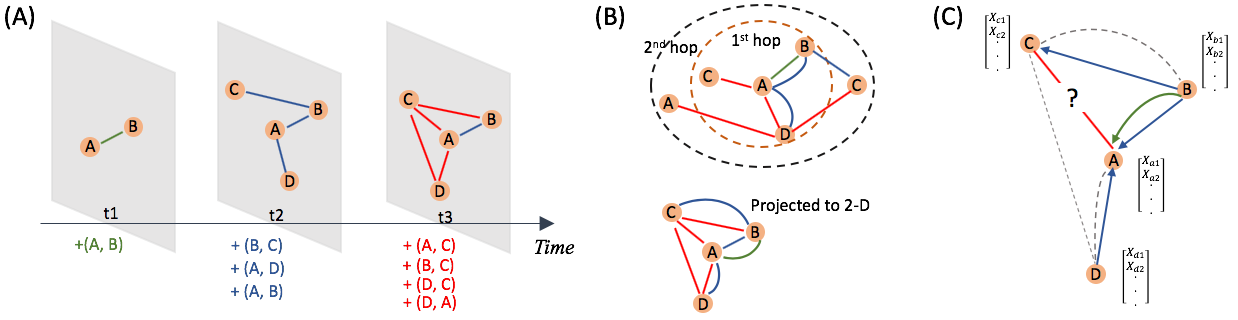
Figure 1: Visual illustration for several complications from the temporal graphs. (A). The generation process of a temporal graph and its snapshots. It is obvious that the static graphs in the snapshots only reflect partial temporal information. (B). The final state of the temporal graph when projected to the time-independent 2-D plane. Other than the missing temporal information, the multi-edge situation arises as well. (C). When predicting the link between node A and C at time $t_{3}$, the message-passing paths should be subject to temporal contraints. The solid lines give the appropriate directions, and the dashed lines violates the temporal constraints.

2 Related Work

Graph representation learning. Spectral graph embedding models operate on the graph spectral domain by approximating, projecting or expanding the graph Laplacian (Kipf & Welling, 2016a; Henaff et al., 2015; Defferrard et al., 2016). Since their training and inference are conditioned on the specific graph spectrum, they are not directly extendable to temporal graphs. Non-spectral approaches, such as GAT, GraphSAGE and MoNET, (Monti et al., 2017) rely on the localized neighbourhood aggregations and thus are not restricted to the training graph. GraphSAGE and GAT also have the flexibility to handle evolving graphs inductively. To extend classical graph representation learning approaches to the temporal domain, several attempts have been done by cropping the temporal graph into a sequence of graph snapshots (Li et al., 2018; Goyal et al., 2018; Rahman et al., 2018; Xu et al., 2019b), and some others work with temporally persistent node (edges) (Trivedi et al., 2018; Ma et al., 2018). Nguyen et al. (2018) proposes a node embedding method based on temporal random walk and reported state-of-the-art performances. However, their approach only generates embeddings for the final state of temporal graph and can not directly apply to the inductive setting.

Self-attention mechanism. Self-attention mechanisms often have two components: the embedding layer and the attention layer. The embedding layer takes an ordered entity sequence as input. Self-attention uses the positional encoding, i.e. each position $k$ is equipped with a vector $\mathbf{p}_{k}$ (fixed or learnt) which is shared for all sequences. For the entity sequence $\mathbf{e}=(e_{1},\ldots,e_{l})$, the embedding layer takes the sum or concatenation of entity embeddings (or features) ($\mathbf{z}\in\mathbb{R}^{d}$) and their positional encodings as input:

$$\mathbf{Z}_{\mathbf{e}}=\big{[}\mathbf{z}_{e_{1}}+\mathbf{p}_{1},\ldots,\mathbf{z}_{e_{1}}+\mathbf{p}_{l}\big{]}^{\intercal}\in\mathbb{R}^{l\times d},\,\text{or}\quad\mathbf{Z}_{\mathbf{e}}=\big{[}\mathbf{z}_{e_{1}}||\mathbf{p}_{1},\ldots,\mathbf{z}_{e_{1}}||\mathbf{p}_{l}\big{]}^{\intercal}\in\mathbb{R}^{l\times(d+d_{\text{pos}})}.$$ (1)

where $||$ denotes concatenation operation and $d_{\text{pos}}$ is the dimension for positional encoding. Self-attention layers can be constructed using the scaled dot-product attention, which is defined as:

$$\text{Attn}\big{(}\mathbf{Q},\mathbf{K},\mathbf{V}\big{)}=\text{softmax}\Big{(}\frac{\mathbf{Q}\mathbf{K}^{\intercal}}{\sqrt{d}}\Big{)}\mathbf{V},$$ (2)

where $\mathbf{Q}$ denotes the ’queries’, $\mathbf{K}$ the ’keys’ and $\mathbf{V}$ the ’values’. In Vaswani et al. (2017), they are treated as projections of the output $\mathbf{Z}_{\mathbf{e}}$: $\mathbf{Q}=\mathbf{Z}_{\mathbf{e}}\mathbf{W}_{Q},\quad\mathbf{K}=\mathbf{Z}_{\mathbf{e}}\mathbf{W}_{K},\quad\mathbf{V}=\mathbf{Z}_{\mathbf{e}}\mathbf{W}_{V},$ where $\mathbf{W}_{Q}$, $\mathbf{W}_{K}$ and $\mathbf{W}_{V}$ are the projection matrices. Since each row of $\mathbf{Q}$, $\mathbf{K}$ and $\mathbf{V}$ represents an entity, the dot-product attention takes a weighted sum of the entity ’values’ in $\mathbf{V}$ where the weights are given by the interactions of entity ’query-key’ pairs. The hidden representation for the entity sequence under the dot-product attention is then given by $h_{\mathbf{e}}=\text{Attn}(\mathbf{Q},\mathbf{K},\mathbf{V})$.

3 Temporal Graph Attention Network Architecture

We first derive the mapping from time domain to the continuous differentiable functional domain as the functional time encoding such that resulting formulation is compatible with self-attention mechanism as well as the backpropagation-based optimization frameworks. The same idea was explored in a concurrent work (Xu et al., 2019a). We then present the temporal graph attention layer and show how it can be naturally extended to incorporate the edge features.

3.1 Functional time encoding

Recall that our starting point is to obtain a continuous functional mapping $\Phi:T\to\mathbb{R}^{d_{T}}$ from time domain to the $d_{T}$-dimensional vector space to replace the positional encoding in (1). Without loss of generality, we assume that the time domain can be represented by the interval starting from origin: $T=[0,t_{\max}]$, where $t_{\max}$ is determined by the observed data. For the inner-product self-attention in (2), often the ’key’ and ’query’ matrices ($\mathbf{K}$, $\mathbf{Q}$) are given by identity or linear projection of $\mathbf{Z}_{\mathbf{e}}$ defined in (1), leading to terms that only involve inner-products between positional (time) encodings. Consider two time points $t_{1},t_{2}$ and inner product between their functional encodings $\big{\langle}\Phi(t_{1}),\Phi(t_{2})\big{\rangle}$. Usually, the relative timespan, rather than the absolute value of time, reveals critical temporal information. Therefore, we are more interested in learning patterns related to the timespan of $|t_{2}-t_{1}|$, which should be ideally expressed by $\big{\langle}\Phi(t_{1}),\Phi(t_{2})\big{\rangle}$ to be compatible with self-attention.

Formally, we define the temporal kernel $\mathcal{K}:T\times T\to\mathbb{R}$ with $\mathcal{K}(t_{1},t_{2}):=\big{\langle}\Phi(t_{1}),\Phi(t_{2})\big{\rangle}$ and $\mathcal{K}(t_{1},t_{2})=\psi(t_{1}-t_{2})$, $\forall t_{1},t_{2}\in T$ for some $\psi:[-t_{\max},t_{\max}]\to\mathbb{R}$. The temporal kernel is then translation-invariant, since $\mathcal{K}(t_{1}+c,t_{2}+c)=\psi(t_{1}-t_{2})=\mathcal{K}(t_{1},t_{2})$ for any constant $c$. Generally speaking, functional learning is extremely complicated since it operates on infinite-dimensional spaces, but now we have transformed the problem into learning the temporal kernel $\mathcal{K}$ expressed by $\Phi$. Nonetheless, we still need to figure out an explicit parameterization for $\Phi$ in order to conduct efficient gradient-based optimization. Classical harmonic analysis theory, i.e. the Bochner’s theorem, motivates our final solution. We point out that the temporal kernel $\mathcal{K}$ is positive-semidefinite (PSD) and continuous, since it is defined via Gram matrix and the mapping $\Phi$ is continuous. Therefore, the kernel $\mathcal{K}$ defined above satisfy the assumptions of the Bochner’s theorem, which we state below.

Theorem 1 (Bochner’s Theorem).

A continuous, translation-invariant kernel $\mathcal{K}(\mathbf{x},\mathbf{y})=\psi(\mathbf{x}-\mathbf{y})$ on $\mathbb{R}^{d}$ is positive definite if and only if there exists a non-negative measure on $\mathbb{R}$ such that $\psi$ is the Fourier transform of the measure.

Consequently, when scaled properly, our temporal kernel $\mathcal{K}$ have the alternate expression:

$$\mathcal{K}(t_{1},t_{2})=\psi(t_{1},t_{2})=\int_{\mathbb{R}}e^{i\omega(t_{1}-t_{2})}p(\omega)d\omega=\mathbb{E}_{\omega}[\xi_{\omega}(t_{1})\xi_{\omega}(t_{2})^{*}],$$ (3)

where $\xi_{\omega}(t)=e^{i\omega t}$. Since the kernel $\mathcal{K}$ and the probability measure $p(\omega)$ are real, we extract the real part of (3) and obtain:

$$\mathcal{K}(t_{1},t_{2})=\mathbb{E}_{\omega}\big{[}\cos(\omega(t_{1}-t_{2}))\big{]}=\mathbb{E}_{\omega}\big{[}\cos(\omega t_{1})\cos(\omega t_{2})+\sin(\omega t_{1})\sin(\omega t_{2})\big{]}.$$ (4)

The above formulation suggests approximating the expectation by the Monte Carlo integral (Rahimi & Recht, 2008), i.e. $\mathcal{K}(t_{1},t_{2})\approx\frac{1}{d}\sum_{i=1}^{d}\cos(\omega_{i}t_{1})\cos(\omega_{i}t_{2})+\sin(\omega_{i}t_{1})\sin(\omega_{i}t_{2})$, with $\omega_{1},\ldots,\omega_{d}\stackrel{{\scriptstyle\text{i.i.d}}}{{\sim}}p(\omega)$. Therefore, we propose the finite dimensional functional mapping to $\mathbb{R}^{d}$ as:

$$t\mapsto\Phi_{d}(t):=\sqrt{\frac{1}{d}}\big{[}\cos(\omega_{1}t),\sin(\omega_{1}t),\ldots,\cos(\omega_{d}t),\sin(\omega_{d}t)\big{]},$$ (5)

and it is easy to show that $\big{\langle}\Phi_{d}(t_{1}),\Phi_{d}(t_{2})\big{\rangle}\approx\mathcal{K}(t_{1},t_{2})$. As a matter of fact, we prove the stochastic uniform convergence of $\big{\langle}\Phi_{d}(t_{1}),\Phi_{d}(t_{2})\big{\rangle}$ to the underlying $\mathcal{K}(t_{1},t_{2})$ and shows that it takes only a reasonable amount of samples to achieve proper estimation, which is stated in Claim 1.

Claim 1.

Let $p(\omega)$ be the corresponding probability measure stated in Bochner’s Theorem for kernel function $\mathcal{K}$. Suppose the feature map $\Phi$ is constructed as described above using samples $\{\omega_{i}\}_{i=1}^{d}$, then we only need $d=\Omega\big{(}\frac{1}{\epsilon^{2}}\log\frac{\sigma_{p}^{2}t_{\max}}{\epsilon}\big{)}$ samples to have

$$\sup_{t_{1},t_{2}\in T}\big{|}\Phi_{d}(t_{1})^{{}^{\prime}}\Phi_{d}(t_{2})-\mathcal{K}(t_{1},t_{2})\big{|}<\epsilon\,\text{with any probability for }\forall\epsilon>0,$$

where $\sigma_{p}^{2}$ is the second momentum with respect to $p(\omega)$.

The proof is provided in supplement material.

By applying Bochner’s theorem, we convert the problem of kernel learning to distribution learning, i.e. estimating the $p(\omega)$ in Theorem 1. A straightforward solution is to apply the reparameterization trick by using auxiliary random variables with a known marginal distribution as in variational autoencoders (Kingma & Welling, 2013). However, the reparameterization trick is often limited to certain distributions such as the ’local-scale’ family, which may not be rich enough for our purpose. For instance, when $p(\omega)$ is multimodal it is difficult to reconstruct the underlying distribution via direct reparameterizations. An alternate approach is to use the inverse cumulative distribution function (CDF) transformation. Rezende & Mohamed (2015) propose using parameterized normalizing flow, i.e. a sequence of invertible transformation functions, to approximate arbitrarily complicated CDF and efficiently sample from it. Dinh et al. (2016) further considers stacking bijective transformations, known as affine coupling layer, to achieve more effective CDF estimation. The above methods learns the inverse CDF function $F^{-1}_{\theta}(.)$ parameterized by flow-based networks and draw samples from the corresponding distribution. On the other hand, if we consider an non-parameterized approach for estimating distribution, then learning $F^{-1}(.)$ and obtain $d$ samples from it is equivalent to directly optimizing the $\{\omega_{1},\ldots,\omega_{d}\}$ in (4) as free model parameters. In practice, we find these two approaches to have highly comparable performances (see supplement material). Therefore we focus on the non-parametric approach, since it is more parameter-efficient and has faster training speed (as no sampling during training is required).

The above functional time encoding is fully compatible with self-attention, thus they can replace the positional encodings in (1) and their parameters are jointly optimized as part of the whole model.

3.2 Temporal graph attention layer

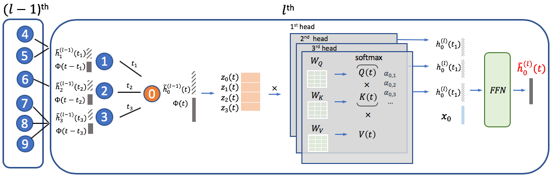
Figure 2: The architecture of the $l^{th}$ TGAT layer with $k=3$ attention heads for node $v_{0}$ at time $t$.

We use $v_{i}$ and $\mathbf{x}_{i}\in\mathbb{R}^{d_{0}}$ to denote node $i$ and its raw node features. The proposed TGAT architecture depends solely on the temporal graph attention layer (TGAT layer). In analogy to GraphSAGE and GAT, the TGAT layer can be thought of as a local aggregation operator that takes the temporal neighborhood with their hidden representations (or features) as well as timestamps as input, and the output is the time-aware representation for target node at any time point $t$. We denote the hidden representation output for node $i$ at time $t$ from the $l^{th}$ layer as $\tilde{\mathbf{h}}^{(l)}_{i}(t)$.

Similar to GAT, we perform the masked self-attention to take account of the structural information (Veličković et al., 2017). For node $v_{0}$ at time $t$, we consider its neighborhood $\mathcal{N}(v_{0};t)=\{v_{1},\ldots,v_{N}\}$ such that the interaction between $v_{0}$ and $v_{i}\in\mathcal{N}(v_{0};t)$, which takes place at time $t_{i}$, is prior to $t$. The input of TGAT layer is the neighborhood information $\mathbf{Z}=\big{\{}\tilde{\mathbf{h}}^{(l-1)}_{1}(t_{1}),\ldots,\tilde{\mathbf{h}}^{(l-1)}_{N}(t_{N})\big{\}}$ and the target node information with some time point $\big{(}\tilde{\mathbf{h}}^{(l-1)}_{0}(t),t\big{)}$. When $l=1$, i.e. for the first layer, the inputs are just raw node features. The layer produces the time-aware representation of target node $v_{0}$ at time $t$, denoted by $\tilde{\mathbf{h}}^{(l)}_{0}(t)$, as its output. Due to the translation-invariant assumption for the temporal kernel, we can alternatively use $\{t-t_{1},\ldots,t-t_{N}\}$ as interaction times, since $|t_{i}-t_{j}|=\big{|}(t-t_{i})-(t-t_{j})\big{|}$ and we only care for the timespan.

In line with original self-attention mechanism, we first obtain the entity-temporal feature matrix as

$$\mathbf{Z}(t)=\Big{[}\tilde{\mathbf{h}}^{(l-1)}_{0}(t)||\Phi_{d_{T}}(0),\tilde{\mathbf{h}}^{(l-1)}_{1}(t_{1})||\Phi_{d_{T}}(t-t_{1}),\ldots,\tilde{\mathbf{h}}^{(l-1)}_{N}(t_{N})||\Phi_{d_{T}}(t-t_{N})\Big{]}^{\intercal}\,\text{(or use sum)}$$ (6)

and forward it to three different linear projections to obtain the ’query’, ’key’ and ’value’:

$$\mathbf{q}(t)=\big{[}\mathbf{Z}(t)\big{]}_{0}\mathbf{W}_{Q},\,\mathbf{K}(t)=\big{[}\mathbf{Z}(t)\big{]}_{1:N}\mathbf{W}_{K},\,\mathbf{V}(t)=\big{[}\mathbf{Z}(t)\big{]}_{1:N}\mathbf{W}_{V},$$

where $\mathbf{W}_{Q},\mathbf{W}_{K},\mathbf{W}_{V}\in\mathbb{R}^{(d+d_{T})\times d_{h}}$ are the weight matrices that are employed to capture the interactions between time encoding and node features. For notation simplicity, in the following discussion we treat the dependence of the intermediate outputs on target time $t$ as implicit. The attention weights $\{\alpha_{i}\}_{i=1}^{N}$ of the softmax function output in (2) is given by: $\alpha_{i}=\exp\big{(}\mathbf{q}^{\intercal}\mathbf{K}_{i}\big{)}/\Big{(}\sum_{q}\exp\big{(}\mathbf{q}^{\intercal}\mathbf{K}_{q}\big{)}\Big{)}$. The attention weight $\alpha_{i}$ reveals how node $i$ attends to the features of node $v_{0}$ within the topological structure defined as $\mathcal{N}(v_{0};t)$ after accounting for their interaction time with $v_{0}$. The self-attention therefore captures the temporal interactions with both node features and topological features and defines a local temporal aggregation operator on graph. The hidden representation for any node $v_{i}\in\mathcal{N}(v_{0};t)$ is given by: $\alpha_{i}\mathbf{V}_{i}$. The mechanism can be effectively shared across all nodes for any time point. We then take the row-wise sum from the above dot-product self-attention output as the hidden neighborhood representations, i.e.

$$\mathbf{h}(t)=\text{Attn}\big{(}\mathbf{q}(t),\mathbf{K}(t),\mathbf{V}(t)\big{)}\in\mathbb{R}^{d_{h}}.$$

To combine neighbourhood representation with the target node features, we adopt the same practice from GraphSAGE and concatenate the neighbourhood representation with the target node’s feature vector $\mathbf{z}_{0}$. We then pass it to a feed-forward neural network to capture non-linear interactions between the features as in (Vaswani et al., 2017):

$$\begin{split}&\tilde{\mathbf{h}}^{(l)}_{0}(t)=\text{FFN}\Big{(}\mathbf{h}(t)||\mathbf{x}_{0}\Big{)}\equiv\text{ReLU}\Big{(}[\mathbf{h}(t)||\mathbf{x}_{0}]\mathbf{W}^{(l)}_{0}+\mathbf{b}^{(l)}_{0}\Big{)}\mathbf{W}^{(l)}_{1}+\mathbf{b}^{(l)}_{1},\\ &\mathbf{W}^{(l)}_{0}\in\mathbb{R}^{(d_{h}+d_{0})\times d_{f}},\mathbf{W}^{(l)}_{1}\in\mathbb{R}^{d_{f}\times d},\mathbf{b}^{(l)}_{0}\in\mathbb{R}^{d_{f}},\mathbf{b}^{(l)}_{1}\in\mathbb{R}^{d},\end{split}$$

where $\tilde{\mathbf{h}}^{(l)}_{0}(t)\in\mathbb{R}^{d}$ is the final output representing the time-aware node embedding at time $t$ for the target node. Therefore, the TGAT layer can be implemented for node classification task using the semi-supervised learning framework proposed in Kipf & Welling (2016a) as well as the link prediction task with the encoder-decoder framework summarized by Hamilton et al. (2017b).

Veličković et al. (2017) suggests that using multi-head attention improves performances and stabilizes training for GAT. For generalization purposes, we also show that the proposed TGAT layer can be easily extended to the multi-head setting. Consider the dot-product self-attention outputs from a total of $k$ different heads, i.e. $\mathbf{h}^{(i)}\equiv\text{Attn}^{(i)}\big{(}\mathbf{q}(t),\mathbf{K}(t),\mathbf{V}(t)\big{)}$, $i=1,\ldots,k$. We first concatenate the $k$ neighborhood representations into a combined vector and then carry out the same procedure:

$$\tilde{\mathbf{h}}^{(l)}_{0}(t)=\text{FFN}\Big{(}\mathbf{h}^{(1)}(t)||\ldots||\mathbf{h}^{(k)}(t)||\mathbf{x}_{0}\Big{)}.$$

Just like GraphSAGE, a single TGAT layer aggregates the localized one-hop neighborhood, and by stacking $L$ TGAT layers the aggregation extends to $L$ hops. Similar to GAT, out approach does not restrict the size of neighborhood. We provide a graphical illustration of our TGAT layer in Figure 2.

3.3 Extension to incorporate Edge Features

We show that the TGAT layer can be naturally extended to handle edge features in a message-passing fashion. Simonovsky & Komodakis (2017) and Wang et al. (2018b) modify classical spectral-based graph convolutional networks to incorporate edge features. Battaglia et al. (2018) propose general graph neural network frameworks where edges features can be processed. For temporal graphs, we consider the general setting where each dynamic edge is associated with a feature vector, i.e. the interaction between $v_{i}$ and $v_{j}$ at time $t$ induces the feature vector $\mathbf{x}_{i,j}(t)$. To propagate edge features during the TGAT aggregation, we simply extend the $\mathbf{Z}(t)$ in (6) to:

$$\mathbf{Z}(t)=\Big{[}\ldots,\tilde{\mathbf{h}}^{(l-1)}_{i}(t_{i})||\mathbf{x}_{0,i}(t_{i})||\Phi_{d_{T}}(t-t_{i}),\ldots\Big{]}\,\text{ (or use summation),}$$ (7)

such that the edge information is propagated to the target node’s hidden representation, and then passed on to the next layer (if exists). The remaining structures stay the same as in Section 3.2.

3.4 Temporal sub-graph batching

Stacking $L$ TGAT layers is equivalent to aggregate over the $L$-hop neighborhood. For each $L$-hop sub-graph that is constructed during the batch-wise training, all message passing directions must be aligned with the observed chronological orders. Unlike the non-temporal setting where each edge appears only once, in temporal graphs two node can have multiple interactions at different time points. Whether or not to allow loops that involve the target node should be judged case-by-case. Sampling from neighborhood, or known as neighborhood dropout, may speed up and stabilize model training. For temporal graphs, neighborhood dropout can be carried uniformly or weighted by the inverse timespan such that more recent interactions has higher probability of being sampled.

3.5 Comparisons to related work

The functional time encoding technique and TGAT layer introduced in Section 3.1 and 3.2 solves several critical challenges, and the TGAT network intrinsically connects to several prior methods.

• Instead of cropping temporal graphs into a sequence of snapshots or constructing time-constraint random walks, which inspired most of the current temporal graph embedding methods, we directly learn the functional representation of time. The proposed approach is motivated by and thus fully compatible with the well-established self-attention mechanism. Also, to the best of our knowledge, no previous work has discussed the temporal-feature interactions for temporal graphs, which is also considered in our approach.

• The TGAT layer is computationally efficient compared with RNN-based models, since the masked self-attention operation is parallelizable, as suggested by Vaswani et al. (2017). The per-batch time complexity of the TGAT layer with $k$ heads and $l$ layers can be expressed as $O\big{(}(k\tilde{N})^{l}\big{)}$ where $\tilde{N}$ is the average neighborhood size, which is comparable to GAT. When using multi-head attention, the computation for each head can be parallelized as well.

• The inference with TGAT is entirely inductive. With an explicit functional expression $\tilde{h}(t)$ for each node, the time-aware node embeddings can be easily inferred for any timestamp via a single network forward pass. Similarity, whenever the graph is updated, the embeddings for both unseen and observed nodes can be quickly inferred in an inductive fashion similar to that of GraphSAGE, and the computations can be parallelized across all nodes.

• GraphSAGE with mean pooling (Hamilton et al., 2017a) can be interpreted as a special case of the proposed method, where the temporal neighborhood is aggregated with equal attention coefficients. GAT is like the time-agnostic version of our approach but with a different formulation for self-attention, as they refer to the work of Bahdanau et al. (2014). We discuss the differences in detail in the Appendix. It is also straightforward to show our connections with the menory networks (Sukhbaatar et al., 2015) by thinking of the temporal neighborhoods as memory. The techniques developed in our work may also help adapting GAT and GraphSAGE to temporal settings as we show in our experiments.

4 Experiment and Results

We test the performance of the proposed method against a variety of strong baselines (adapted for temporal settings when possible) and competing approaches, for both the inductive and transductive tasks on two benchmark and one large-scale industrial dataset.

4.1 Datasets

Real-world temporal graphs consist of time-sensitive node interactions, evolving node labels as well as new nodes and edges. We choose the following datasets which contain all scenarios.

Reddit dataset. We use the data from active users and their posts under subreddits, leading to a temporal graph with 11,000 nodes, $\sim$700,000 temporal edges and dynamic labels indicating whether a user is banned from posting. The user posts are transformed into edge feature vectors.

Wikipedia dataset. We use the data from top edited pages and active users, yielding a temporal graph $\sim$9,300 nodes and around 160,000 temporal edges. Dynamic labels indicate if users are temporarily banned from editing. The user edits are also treated as edge features.

Industrial dataset. We choose 70,000 popular products and 100,000 active customers as nodes from the online grocery shopping website and use the customer-product purchase as temporal edges ($\sim$2 million). The customers are tagged with labels indicating if they have a recent interest in dietary products. Product features are given by the pre-trained product embeddings (Xu et al., 2020).

We do the chronological train-validation-test split with 70%-15%-15% according to node interaction timestamps. The dataset and preprocessing details are provided in the supplement material.

4.2 Transductive and inductive learning tasks

Since the majority of temporal information is reflected via the timely interactions among nodes, we choose to use a more revealing link prediction setup for training. Node classification is then treated as the downstream task using the obtained time-aware node embeddings as input.

Transductive task examines embeddings of the nodes that have been observed in training, via the future link prediction task and the node classification. To avoid violating temporal constraints, we predict the links that strictly take place posterior to all observations in the training data.

Inductive task examines the inductive learning capability using the inferred representations of unseen nodes, by predicting the future links between unseen nodes and classify them based on their inferred embedding dynamically. We point out that it suffices to only consider the future sub-graph for unseen nodes since they are equivalent to new graphs under the non-temporal setting.

As for the evaluation metrics, in the link prediction tasks, we first sample an equal amount of negative node pairs to the positive links and then compute the average precision (AP) and classification accuracy. In the downstream node classification tasks, due to the label imbalance in the datasets, we employ the area under the ROC curve (AUC).

Dataset	Reddit		Wikipedia		Industrial
Metric	Accuracy	AP	Accuracy	AP	Accuracy	AP
GAE	74.31 (0.5)	93.23 (0.3)	72.85 (0.7)	91.44 (0.1)	68.92 (0.3)	81.15 (0.2)
VAGE	74.19 (0.4)	92.92 (0.2)	78.01 (0.3)	91.34 (0.3)	67.81 (0.4)	80.87 (0.3)
DeepWalk	71.43 (0.6)	83.10 (0.5)	76.67 (0.5)	90.71 (0.6)	65.87 (0.3)	80.93 (0.2)
Node2vec	72.53 (0.4)	84.58 (0.5)	78.09 (0.4)	91.48 (0.3)	66.64 (0.3)	81.39 (0.3)
CTDNE	73.76 (0.5)	91.41 (0.3)	79.42 (0.4)	92.17 (0.5)	67.81 (0.3)	80.95 (0.5)
GAT	92.14 (0.2)	97.33 (0.2)	87.34 (0.3)	94.73 (0.2)	69.58 (0.4)	81.51 (0.2)
GAT+T	92.47 (0.2)	97.62 (0.2)	87.57 (0.2)	95.14 (0.4)	70.15 (0.3)	82.66 (0.4)
GraphSAGE	92.31(0.2)	97.65 (0.2)	85.93 (0.3)	93.56 (0.3)	70.19 (0.2)	83.27 (0.3)
GraphSAGE+T	92.58 (0.2)	97.89 (0.3)	86.31 (0.3)	93.72 (0.3)	71.84 (0.3)	84.95 (0.)
Const-TGAT	91.39 (0.2)	97.86 (0.2)	86.03 (0.4)	93.50 (0.3)	68.52 (0.2)	81.91 (0.3)
TGAT	92.92 (0.3)	98.12 (0.2)	88.14 (0.2)	95.34 (0.1)	73.28 (0.2)	86.32 (0.1)

Table 1: Transductive learning task results for predicting future edges of nodes that have been observed in training data. All results are converted to percentage by multiplying by 100, and the standard deviations computed over ten runs (in parenthesis). The best and second-best results in each column are highlighted in bold font and underlined. GraphSAGE is short for GraphSAGE-LSTM.

Dataset	Reddit		Wikipedia		Industrial
Metric	Accuracy	AP	Accuracy	AP	Accuracy	AP
GAT	89.86 (0.2)	95.37 (0.3)	82.36 (0.3)	91.27 (0.4)	68.28 (0.2)	79.93 (0.3)
GAT+T	90.44 (0.3)	96.31 (0.3)	84.82 (0.3)	93.57 (0.3)	69.51 (0.3)	81.68 (0.3)
GraphSAGE	89.43 (0.1)	96.27 (0.2)	82.43 (0.3)	91.09 (0.3)	67.49 (0.2)	80.54 (0.3)
GraphSAGE+T	90.07 (0.2)	95.83 (0.2)	84.03 (0.4)	92.37 (0.5)	69.66 (0.3)	82.74 (0.3)
Const-TGAT	88.28 (0.3)	94.12 (0.2)	83.60 (0.4)	91.93 (0.3)	65.87 (0.3)	77.03 (0.4)
TGAT	90.73 (0.2)	96.62 (0.3)	85.35 (0.2)	93.99 (0.3)	72.08 (0.3)	84.99 (0.2)

Table 2: Inductive learning task results for predicting future edges of unseen nodes.

4.3 Baselines

Transductive task: for link prediction of observed nodes, we choose the compare our approach with the state-of-the-art graph embedding methods: GAE and VGAE (Kipf & Welling, 2016b). For complete comparisons, we also include the skip-gram-based node2vec (Grover & Leskovec, 2016) as well as the spectral-based DeepWalk model (Perozzi et al., 2014), using the same inner-product decoder as GAE for link prediction. The CDTNE model based on the temporal random walk has been reported with superior performance on transductive learning tasks (Nguyen et al., 2018), so we include CDTNE as the representative for temporal graph embedding approaches.

Inductive task: few approaches are capable of managing inductive learning on graphs even in the non-temporal setting. As a consequence, we choose GraphSAGE and GAT as baselines after adapting them to the temporal setting. In particular, we equip them with the same temporal sub-graph batching describe in Section 3.4 to maximize their usage on temporal information. Also, we implement the extended version for the baselines to include edge features in the same way as ours (in Section 3.3). We experiment on different aggregation functions for GraphSAGE, i.e. GraphSAGE-mean, GraphSAGE-pool and GraphSAGE-LSTM. In accordance with the original work of Hamilton et al. (2017a), GraphSAGE-LSTM gives the best validation performance among the three approaches, which is reasonable under temporal setting since LSTM aggregation takes account of the sequential information. Therefore we report the results of GraphSAGE-LSTM.

In addition to the above baselines, we implement a version of TGAT with all temporal attention weights set to equal value (Const-TGAT). Finally, to show that the superiority of our approach owes to both the time encoding and the network architecture, we experiment with the enhanced GAT and GraphSAGE-mean by concatenating the proposed time encoding to the original features during temporal aggregations (GAT+T and GraphSAGE+T).

Figure 3: Results of node classification task in the ablation study.

Dataset	Reddit	Wikipedia	Industrial
GAE	58.39 (0.5)	74.85 (0.6)	76.59 (0.3)
VGAE	57.98 (0.6)	73.67 (0.8)	75.38 (0.4)
CTDNE	59.43 (0.6)	75.89 (0.5)	78.36 (0.5)
GAT	64.52 (0.5)	82.34 (0.8)	87.43 (0.4)
GAT+T	64.76 (0.6)	82.95 (0.7)	88.24 (0.5)
GraphSAGE	61.24 (0.6)	82.42 (0.7)	88.28 (0.3)
GraphSAGE+T	62.31 (0.7)	82.87 (0.6)	89.81 (0.3)
Const-TGAT	60.97 (0.5)	75.18 (0.7)	82.59 (0.6)
TGAT	65.56 (0.7)	83.69 (0.7)	92.31 (0.3)

Table 3: Dynamic node classification task results, where the reported metric is the AUC.

4.4 Experiment setup

We use the time-sensitive link prediction loss function for training the $l$-layer TGAT network:

$$\ell=\sum_{(v_{i},v_{j},t_{ij})\in\mathcal{E}}-\log\Big{(}\sigma\big{(}-\tilde{\mathbf{h}}_{i}^{l}(t_{ij})^{\intercal}\tilde{\mathbf{h}}_{j}^{l}(t_{ij})\big{)}\Big{)}-Q.\mathbb{E}_{v_{q}\sim P_{n}(v)}\log\Big{(}\sigma\big{(}\tilde{\mathbf{h}}_{i}^{l}(t_{ij})^{\intercal}\tilde{\mathbf{h}}_{q}^{l}(t_{ij})\big{)}\Big{)},$$ (8)

where the summation is over the observed edges on $v_{i}$ and $v_{j}$ that interact at time $t_{ij}$, and $\sigma(.)$ is the sigmoid function, $Q$ is the number of negative samples and $P_{n}(v)$ is the negative sampling distribution over the node space. As for tuning hyper-parameters, we fix the node embedding dimension and the time encoding dimension to be the original feature dimension for simplicity, and then select the number of TGAT layers from {1,2,3}, the number of attention heads from {1,2,3,4,5}, according to the link prediction AP score in the validation dataset. Although our method does not put restriction on the neighborhood size during aggregations, to speed up training, specially when using the multi-hop aggregations, we use neighborhood dropout (selected among $p=${0.1, 0.3, 0.5}) with the uniform sampling. During training, we use $0.0001$ as learning rate for Reddit and Wikipedia dataset and $0.001$ for the industrial dataset, with Glorot initialization and the Adam SGD optimizer. We do not experiment on applying regularization since our approach is parameter-efficient and only requires $\Omega\big{(}(d+d_{T})d_{h}+(d_{h}+d_{0})d_{f}+d_{f}d\big{)}$ parameters for each attention head, which is independent of the graph and neighborhood size. Using two TGAT layers and two attention heads with dropout rate as 0.1 give the best validation performance. For inference, we inductively compute the embeddings for both the unseen and observed nodes at each time point that the graph evolves, or when the node labels are updated. We then use these embeddings as features for the future link prediction and dynamic node classifications with multilayer perceptron.

We further conduct ablation study to demonstrate the effectiveness of the proposed functional time encoding approach. We experiment on abandoning time encoding or replacing it with the original positional encoding (both fixed and learnt). We also compare the uniform neighborhood dropout to sampling with inverse timespan (where the recent edges are more likely to be sampled), which is provided in supplement material along with other implementation details and setups for baselines.

4.5 Results

The results in Table 1 and Table 2 demonstrates the state-of-the-art performances of our approach on both transductive and inductive learning tasks. In the inductive learning task, our TGAT network significantly improves upon the the upgraded GraphSAGE-LSTM and GAT in accuracy and average precision by at least 5 % for both metrics, and in the transductive learning task TGAT consistently outperforms all baselines across datasets. While GAT+T and GraphSAGE+T slightly outperform or tie with GAT and GraphSAGE-LSTM, they are nevertheless outperformed by our approach. On one hand, the results suggest that the time encoding have potential to extend non-temporal graph representation learning methods to temporal settings. On the other, we note that the time encoding still works the best with our network architecture which is designed for temporal graphs. Overall, the results demonstrate the superiority of our approach in learning representations on temporal graphs over prior models. We also see the benefits from assigning temporal attention weights to neighboring nodes, where GAT significantly outperforms the Const-TGAT in all three tasks. The dynamic node classification outcome (in Table 3) further suggests the usefulness of our time-aware node embeddings for downstream tasks as they surpass all the baselines. The ablation study results of Figure 3 successfully reveals the effectiveness of the proposed functional time encoding approach in capturing temporal signals as it outperforms the positional encoding counterparts.

4.6 Attention Analysis

To shed some insights into the temporal signals captured by the proposed TGAT, we analyze the pattern of the attention weights $\{\alpha_{ij}(t)\}$ as functions of both time $t$ and node pairs $(i,j)$ in the inference stage. Firstly, we analyze how the attention weights change with respect to the timespans of previous interactions, by plotting the attention weights $\big{\{}\alpha_{jq}(t_{ij})|q\in\mathcal{N}(v_{j};t_{ij})\big{\}}\cup\big{\{}\alpha_{ik}(t_{ij})|k\in\mathcal{N}(v_{i};t_{ij})\big{\}}$ against the timespans $\{t_{ij}-t_{jq}\}\cup\{t_{ij}-t_{ik}\}$ when predicting the link for $(v_{i},v_{j},t_{ij})\in\mathcal{E}$ (Figure 4a). This gives us an empirical estimation on the $\alpha(\Delta t)$, where a smaller $\Delta t$ means a more recent interaction. Secondly, we analyze how the topological structures affect the attention weights as time elapses. Specifically, we focus on the topological structure of the recurring neighbours, by finding out what attention weights the model put on the neighbouring nodes with different number of reoccurrences. Since the functional forms of all $\{\alpha_{ij}(.)\}$ are fixed after training, we are able to feed in different target time $t$ and then record their value on neighbouring nodes with different number of occurrences (Figure 4b). From Figure 4a we observe that TGAT captures the pattern of having less attention on more distant interactions in all three datasets. In Figure 4b, it is obvious that when predicting a more future interaction, TGAT will consider neighbouring nodes who have a higher number of occurrences of more importance. The patterns of the attention weights are meaningful, since the more recent and repeated actions often have larger influence on users’ future interests.

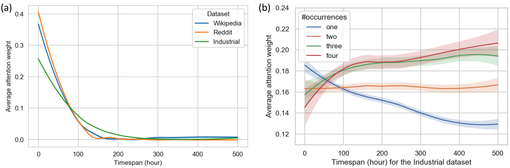
Figure 4: Attention weight analysis. We apply the Loess smoothing method for visualization.

5 Conclusion and future work

We introduce a novel time-aware graph attention network for inductive representation learning on temporal graphs. We adapt the self-attention mechanism to handle the continuous time by proposing a theoretically-grounded functional time encoding. Theoretical and experimental analysis demonstrate the effectiveness of our approach for capturing temporal-feature signals in terms of both node and topological features on temporal graphs. Self-attention mechanism often provides useful model interpretations (Vaswani et al., 2017), which is an important direction of our future work. Developing tools to visualize the evolving graph dynamics and temporal representations efficiently is another important direction for both research and application. Also, the functional time encoding technique has huge potential for adapting other deep learning methods to the temporal graph domain.

Appendix A Appendix

A.1 proof for claim 1

Proof.

The proof is also shown in our concurrent work Xu et al. (2019a). We also provide it here for completeness. To prove the results in Claim 1, we alternatively show that under the same condition,

$$\text{Pr}\big{(}\sup_{t_{1},t_{2}\in T}|\Phi^{\mathcal{B}}_{d}(t_{1})^{{}^{\prime}}\Phi^{\mathcal{B}}_{d}(t_{2})-\mathcal{K}(t_{1},t_{2})|\geq\epsilon\big{)}\leq 4\sigma_{p}\sqrt{\frac{t_{\max}}{\epsilon}}exp\big{(}\frac{-d\epsilon^{2}}{32}\big{)}.$$ (9)

Define the score $S(t_{1},t_{2})=\Phi^{\mathcal{B}}_{d}(t_{1})^{{}^{\prime}}\Phi^{\mathcal{B}}_{d}(t_{2})$. The goal is to derive a uniform upper bound for $s(t_{1},t_{2})-\mathcal{K}(t_{1},t_{2})$. By assumption $S(t_{1},t_{2})$ is an unbiased estimator for $\mathcal{K}(t_{1},t_{2})$, i.e. $E[S(t_{1},t_{2})]=\mathcal{K}(t_{1},t_{2})$. Due to the translation-invariant property of $S$ and $\mathcal{K}$, we let $\Delta(t)\equiv s(t_{1},t_{2})-\mathcal{K}(t_{1},t_{2})$, where $t\equiv t_{1}-t_{2}$ for all $t_{1},t_{2}\in[0,t_{\max}]$. Also we define $s(t_{1}-t_{2}):=S(t_{1},t_{2})$. Therefore $t\in[-t_{\max},t_{\max}]$, and we use $t\in\tilde{T}$ as the shorthand notation. The LHS in (1) now becomes $\text{Pr}\big{(}\sup_{t\in\tilde{T}}|\Delta(t)|\geq\epsilon\big{)}$.

Note that $\tilde{T}\subseteq\cup_{i=0}^{N-1}T_{i}$ with $T_{i}=[-t_{\max}+\frac{2it_{\max}}{N},-t_{\max}+\frac{2(i+1)t_{\max}}{N}]$ for $i=1,\ldots,N$. So $\cup_{i=0}^{N-1}T_{i}$ is a finite cover of $\tilde{T}$. Define $t_{i}=-t_{\max}+\frac{(2i+1)t_{\max}}{N}$, then for any $t\in T_{i}$, $i=1,\ldots,N$ we have

$$\begin{split}|\Delta(t)|&=|\Delta(t)-\Delta(t_{i})+\Delta(t_{i})|\\ &\leq|\Delta(t)-\Delta(t_{i})|+|\Delta(t_{i})|\\ &\leq L_{\Delta}|t-t_{i}|+|\Delta(t_{i})|\\ &\leq L_{\Delta}\frac{2t_{\max}}{N}+|\Delta(t_{i})|,\end{split}$$ (10)

where $L_{\Delta}=\max_{t\in\tilde{T}}\|\nabla\Delta(t)\|$ (since $\Delta$ is differentiable) with the maximum achieved at $t^{*}$. So we may bound the two events separately.

For $|\Delta(t_{i})|$ we simply notice that trigeometric functions are bounded between $[-1,1]$, and therefore $-1\leq\Phi^{\mathcal{B}}_{d}(t_{1})^{{}^{\prime}}\Phi^{\mathcal{B}}_{d}(t_{2})\leq 1$. The Hoeffding’s inequality for bounded random variables immediately gives us:

$$\text{Pr}\big{(}|\Delta(t_{i})|>\frac{\epsilon}{2}\big{)}\leq 2exp(-\frac{d\epsilon^{2}}{16}).$$

So applying the Hoeffding-type union bound to the finite cover gives

$$\text{Pr}(\cup_{i=0}^{N-1}|\Delta(t_{i})|\geq\frac{\epsilon}{2})\leq 2N\exp(-\frac{d\epsilon^{2}}{16})$$ (11)

For the other event we first apply Markov inequality and obtain:

$$\text{Pr}\big{(}L_{\Delta}\frac{2t_{\max}}{N}\geq\frac{\epsilon}{2}\big{)}=\text{Pr}\big{(}L_{\Delta}\geq\frac{\epsilon N}{4t_{\max}}\big{)}\leq\frac{4t_{\max}E[L_{\Delta}^{2}]}{\epsilon N}.$$ (12)

Also, since $E[s(t_{1}-t_{2})]=\psi(t_{1}-t_{2})$, we have

$$E[L_{\Delta}^{2}]=E\|\nabla s(t^{*})-\nabla\psi(t^{*})\|^{2}=E\|\nabla s(t^{*})\|^{2}-E\|\nabla\psi(t^{*})\|^{2}\leq E\|\nabla s(t^{*})\|^{2}=\sigma_{p}^{2},$$ (13)

where $\sigma_{p}^{2}$ is the second momentum with respect to $p(\omega)$.

Combining (11), (12) and (11) gives us:

$$\text{Pr}\big{(}\sup_{t\in\tilde{T}}|\Delta(t)|\geq\epsilon\big{)}\leq 2N\exp(-\frac{d\epsilon^{2}}{16})+\frac{4t_{\max}\sigma_{p}^{2}}{\epsilon N}.$$ (14)

It is straightforward to examine that the RHS of (14) is a convex function of $N$ and is minimized by $N^{*}=\sigma_{p}\sqrt{\frac{2t_{\max}}{\epsilon}}exp(\frac{d\epsilon^{2}}{32})$. Plug $N^{*}$ back to (14) and we obtain (9). We then solve for $d$ according to (9) and obtain the results in Claim 1.

∎

A.2 Comparisons between the attention mechanism of TGAT and GAT

In this part, we provide detailed comparisons between the attention mechanism employed by our proposed TGAT and the GAT proposed by Veličković et al. (2017). Other than the obvious fact that GAT does not handle temporal information, the main difference lies in the formulation of attention weights. While GAT depends on the attention mechanism proposed by Bahdanau et al. (2014), our architecture refers to the self-attention mechanism of Vaswani et al. (2017). Firstly, the attention mechanism used by GAT does not involve the notions of ’query’, ’key’ and ’value’ nor the dot-product formulation introduced in (2). As a consequence, the attention weight between node $v_{i}$ and its neighbor $v_{j}$ is computed via

$$\alpha_{ij}=\frac{\exp\Big{(}\text{LeakyReLU}\big{(}\mathbf{a}^{\intercal}[\mathbf{W}\mathbf{h}_{i}||\mathbf{W}\mathbf{h}_{j}]\big{)}\Big{)}}{\sum_{k\in\mathcal{N}(v_{i})}\exp\Big{(}\text{LeakyReLU}\big{(}\mathbf{a}^{\intercal}[\mathbf{W}\mathbf{h}_{i}||\mathbf{W}\mathbf{h}_{k}]\big{)}\Big{)}},$$

where $\mathbf{a}$ is a weight vector, $\mathbf{W}$ is a weight matrix, $\mathcal{N}(v_{i})$ is the neighorhood set for node $v_{i}$ and $\mathbf{h}_{i}$ is the hidden representation of node $v_{i}$. It is then obvious that their computation of $\alpha_{ij}$ is very different from our approach. In TGAT, after expanding the expressions in Section 3, the attention weight is computed by:

$$\alpha_{ij}(t)=\frac{\exp\Big{(}\big{(}[\tilde{\mathbf{h}}_{i}(t_{i})||\Phi_{d_{T}}(t-t_{i})]\mathbf{W}_{Q}\big{)}^{\intercal}\big{(}[\tilde{\mathbf{h}}_{j}(t_{j})||\Phi_{d_{T}}(t-t_{j})]\mathbf{W}_{K}\big{)}\Big{)}}{\sum_{k\in\mathcal{N}(v_{i};t)}\exp\Big{(}\big{(}[\tilde{\mathbf{h}}_{i}(t_{i})||\Phi_{d_{T}}(t-t_{i})]\mathbf{W}_{Q}\big{)}^{\intercal}\big{(}[\tilde{\mathbf{h}}_{k}(t_{k})||\Phi_{d_{T}}(t-t_{k})]\mathbf{W}_{K}\big{)}\Big{)}}.$$

Intuitively speaking, the attention mechanism of GAT relies on the parameter vector $\mathbf{a}$ and the LeakyReLU(.) to capture the hidden factor interactions between entities in the sequence, while we use the linear transformation followed by the dot-product to capture pair-wise interactions of the hidden factors between entities and the time embeddings. The dot-product formulation is important for our approach. From the theoretical perspective, the time encoding functional form is derived according to the notion of temporal kernel $\mathcal{K}$ and its inner-product decomposition (Section 3). As for the practical performances, we see from Table 1, 2 and 3 that even after we equip GAT with the same time encoding, the performance is still inferior to our TGAT.

A.3 Details on datasets and preprocessing

Reddit dataset: this benchmark dataset contains users interacting with subreddits by posting under the subreddits. The timestamps tell us when the user makes the posts. The dataset uses the posts made in a one-month span, and selects the most active users and subreddits as nodes, giving a total of 11,000 nodes and around 700,000 temporal edges. The user posts have textual features that are transformed into a 172-dimensional vector representing under the linguistic inquiry and word count (LIWC) categories (Pennebaker et al., 2001). The dynamic binary labels indicate if a user is banned from posting under a subreddit. Since node features are not provided in the original dataset, we use the all-zero vector instead.

Wikipedia dataset: the dataset also collects one-month of interactions induced by users’ editing the Wikipedia pages. The the top edited pages and active users are considered, leading to $\sim$9,300 nodes and around 160,000 temporal edges. Similar to the Reddit dataset, we also have the ground-truth dynamic labels on whether a user is banned from editing a Wikipedia page. User edits consist of the textual features and are also converted into 172-dimensional LIWC feature vectors. Node features are also not provided, so we also use the all-zero vector as well.

Industrial dataset: we obtain the large-scale customer-product interaction graph from the online grocery shopping platform grocery.walmart.com. We select $\sim$70,000 most popular products and 100,000 active customers as nodes and use the customer-product purchase interactions over a one-month period as temporal edges ($\sim$2 million). Each purchase interaction is timestamped, which we use to construct the temporal graph. The customers are labelled with business tags, indicating if they are interested in dietary products according to their most recent purchase records. Each product node possesses contextual features containing their name, brand, categories and short description. The previous LIWC categories no longer apply since the product contextual features are not natural sentences. We use product embedding approach (Xu et al., 2020) to embed each product’s contextual features into a 100-dimensional vector space as preprocessing. The user nodes and edges do not possess features.

We then split the temporal graphs chronologically into 70%-15%-15% for training, validation and testing according to the time epochs of edges, as illustrated in Figure 5 with the Reddit dataset. Since all three datasets have a relatively stationary edge count distribution over time, using the 70 and 85 percentile time points to split the dataset results in approximately 70%-15%-15% of total edges, as suggested by Figure 5.

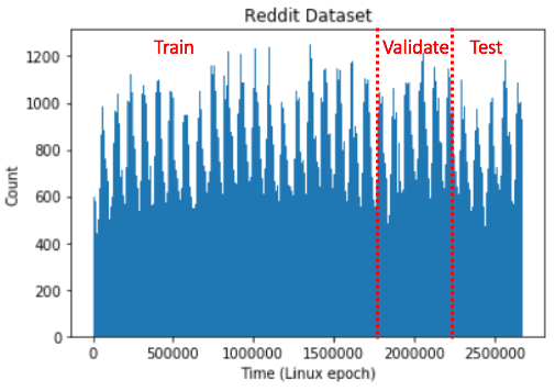
Figure 5: The distribution of temporal edge count for the Reddit dataset, and the illustration on the train-validation-test splitting.

To ensure that an appropriate amount of future edges among the unseen nodes will show up during validation and testing, for each dataset, we randomly sample 10% of nodes, mask them during training and treat them as unseen nodes by only considering their interactions in validation and testing period. This manipulation is necessary since the new nodes that show up during validation and testing period may not have much interaction among themselves. The statistics for the three datasets are summarized in Table 4.

	Reddit	Wikipedia	Industrial
# Nodes	11,000	9,227	170,243
# Edges	672,447	157,474	2,135,762
# Feature dimension	172	172	100
# Feature type	LIWC category vector	LIWC category vector	document embeddings
# Timespan	30 days	30 days	30 days
% Training nodes	90%	90%	90%
% Unseen nodes	10%	10%	10%
% Training edges	$\sim$67%	$\sim$65%	$\sim$64%
% Future edges between observed nodes	$\sim$27%	$\sim$28%	$\sim$29%
% Future edges between unseen nodes	$\sim$6%	$\sim$7%	$\sim$7%
# Nodes with dynamic labels	366	217	5,236
Label type	binary	binary	binary
Positive label meaning	banned from posting	banned from editting	interested in dietary products

Table 4: Data statistics for the three datasets. Since we sample a proportion of unseen nodes, the percentage of the edge statistics reported here are approximations.

Preprocessing.

For the Node2vec and DeepWalk baselines who only take static graphs as input, the graph is constructed using all edges in training data regardless of temporal information. For DeepWalk, we treat the recurrent edges as appearing only once, so the graph is unweighted. Although our approach handles both directed and undirected graphs, for the sake of training stability of the baselines, we treat the graphs as undirected. For Node2vec, we use the count of recurrent edges as their weights and construct the weighted graph. For all three datasets, the obtained graphs in both cases are undirected and do not have isolated nodes. Since we choose from active users and popular items, the graphs are all connected.

For the graph convolutional network baselines, i.e. GAE and VGAE, we construct the same undirected weighted graph as for Node2vec. Since GAE and VGAE do not take edge features as input, we use the posts/edits as user node features. For each user in Reddit and Wikipedia dataset, we take the average of their post/edit feature vectors as the node feature. For the industrial dataset where user features are not available, we use the all-zero feature vector instead.

As for the downstream dynamic node classification task, we use the same training, validation and testing dataset as above. Since we aim at predicting the dynamic node labels, for Reddit and Wikipedia dataset we predict if the user node is banned and for the industrial dataset we predict the customers’ business labels, at different time points. Due to the label imbalance, in each of the batch when training for the node label classifier, we conduct stratified sampling such that the label distributions are similar across batches.

A.4 Experiment Setup for Baselines

For all baselines, we set the node embedding dimension to $d=100$ to keep in accordance with our approach.

Transductive baselines.

Since Node2vec and DeepWalk do not provide room for task-specific manipulation or hacking, we do not modify their default loss function and input format. For both approaches, we select the number of walks among {60,80,100} and the walk-length among {20,30,40} according to the validation AP. Setting number of walks=80 and walk-length=30 give slightly better validation performance compared to others for both approaches. Notice that both Node2vec and DeepWalk use the sigmoid function with embedding inner-products as the decoder to predict neighborhood probabilities. So when predicting whether $v_{i}$ and $v_{j}$ will interact in the future, we use $\sigma(-\mathbf{z}_{i}^{\intercal}\mathbf{z}_{j})$ as the score, where $\mathbf{z}_{i}$ and $\mathbf{z}_{j}$ are the node embeddings. Notice that Node2vec has the extra hyper-parameter $p$ and $q$ which controls the likelihood of immediately revisiting a node in the walk and interpolation between breadth-first strategy and depth-first strategy. After selecting the optimal number of walks and walk-length under $p=1$ and $q=1$, we further tune the different values of $p$ in {0.2,0.4,0.6,0.8,1.0} while fixing $q=1$. According to validation, $p=0.6$ and $0.8$ give comparable optimal performance.

For the GAE and VGAE baselines, we experiment on using one, two and three graph convolutional layers as the encoder (Kipf & Welling, 2016a) and use the $\text{ReLU}(.)$ as the activation function. By referencing the official implementation, we also set the dimension of hidden layers to 200. Similar to previous findings, using two layers gives significant performances to using only one layer. Adding the third layer, on the other hand, shows almost identical results for both models. Therefore the results reported are based on two-layer GCN as the encoder. For GAE, we use the standard inner-product decoder as our approach and optimize over the reconstruction loss, and for VGAE, we restrict the Gaussian latent factor space (Kipf & Welling, 2016b). Since we have eliminated the temporal information when constructing the input, we find that the optimal hyper-parameters selected according to the tuning have similar patterns as in the previous non-temporal settings.

For the temporal network embedding model CTDNE, the walk length for the temporal random walk is also selected among {60,80,100}, where setting walk length to 80 gives slightly better validation outcome. The original paper considers several temporal edge selection (sampling) methods (uniform, linear and exponential) and finds uniform sampling with best performances (Nguyen et al., 2018). Since our setting is similar to theirs, we adopt the uniform sampling approach.

Inductive baselines.

For the GraphSAGE and GAT baselines, as mentioned before, we train the models in an identical way as our approach with the temporal subgraph batching, despite several slight differences. Firstly, the aggregation layers in GraphSAGE usually considers a fixed neighborhood size via sampling, whereas our approach can take an arbitrary neighborhood as input. Therefore, we only consider the most recent $d_{\text{sample}}$ edges during each aggregation for all layers, and we find $d_{\text{sample}}=20$ gives the best performance among {10,15,20,25}. Secondly, GAT implements a uniform neighborhood dropout. We also experiment with the inverse timespan sampling for neighborhood dropout, and find that it gives slightly better performances but at the cost of computational efficiency, especially for large graphs. We consider aggregating over one, two and three-hop neighborhood for both GAT and GraphSAGE. When working with three hops, we only experiment on GraphSAGE with the mean pooling aggregation. In general, using two hops gives comparable performance to using three hops. Notice that computations with three-hop are costly, since the number of edges during aggregation increase exponentially to the number of hops. Thus we stick to using two hops for GraphSAGE, GAT and our approach. It is worth mentioning that when implementing GraphSAGE-LSTM, the input neighborhood sequences of LSTM are also ordered by their interaction time.

Node classification with baselines.

The dynamic node classification with GraphSAGE and GAT can be conducted similarity to our approach, where we inductively compute the most up-to-date node embeddings and then input them as features to an MLP classifier. For the transductive baselines, it is not reasonable to predict the dynamic node labels with only the fixed node embeddings. Instead, we combine the node embedding with the other node embedding it is interacting with when the label changes, e.g. combine the user embedding with the Wikipedia page embedding that the user attempts on editing when the system bans the user. To combine the pair of node embeddings, we experimented on summation, concatenation and bi-linear transformation. Under summation and concatenation, the combined embeddings are then used as input to an MLP classifier, where the bi-linear transformation directly outputs scores for classification. The validation outcomes suggest that using concatenation with MLP yields the best performance.

A.5 Implementation details

Training. We implement Node2vec using the official C code on a 16-core Linux server with 500 Gb memory. DeepWalk is implemented with the official python code. We refer to the PyTorch geometric library for implementing the GAE and VGAE baselines (Fey & Lenssen, 2019). To accommodate the temporal setting and incorporate edges features, we develop off-the-shelf implementation for GraphSAGE and GAT in PyTorch by referencing their original implementations . We also implement our model using PyTorch. All the deep learning models are trained on a machine with one Tesla V100 GPU. We use the Glorot initialization and the Adam SGD optimizer for all models, and apply the early-stopping strategy during training where we terminate the training process if the validation AP score does not improve for 10 epochs.

Downstream node classification. As we discussed before, we use the three-layer MLP as classifier and the (combined) node embeddings as input features from all the experimented approaches, for all three datasets. The MLP is trained with the Glorot initialization and the Adam SGD optimizer in PyTorch as well. The $\ell_{2}$ regularization parameter $\lambda$ is selected in {0.001, 0.01, 0.05, 0.1, 0.2} case-by-case during training. The early-stopping strategy is also employed.

A.6 Sensitivity analysis and extra ablation study

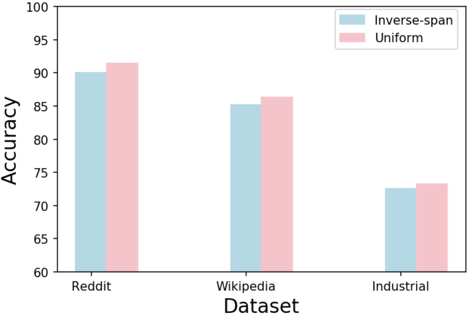
(a) Comparison between uniform and inverse timespan weighted sampling on the link prediction task

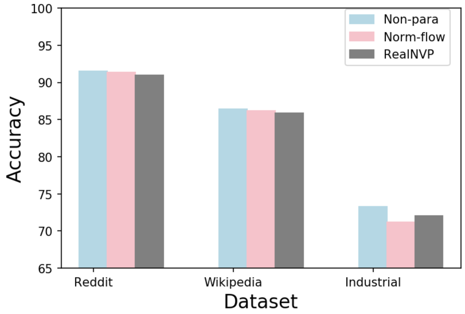
(b) Comparison between three different ways of learning the functional time encoding, on link prediction task.

Figure 6: Extra ablation study.

Firstly, we focus on the output node embedding dimension as well as the functional time encoding dimension in this sensitivity analysis. The reported results are averaged over five runs. We experiment on $d\in\{60,80,100,120,140\}$ and $d_{T}\in\{60,80,100,120,140\}$, and the results are reported in Figure 7(a) and 7(c). The remaining model setups reported in Section 4.4 are untouched when varying $d$ or $d_{T}$. We observe slightly better outcome when increasing either $d$ or $d_{T}$ on the industrial dataset. The patterns on Reddit and Wikipedia dataset are almost identical.

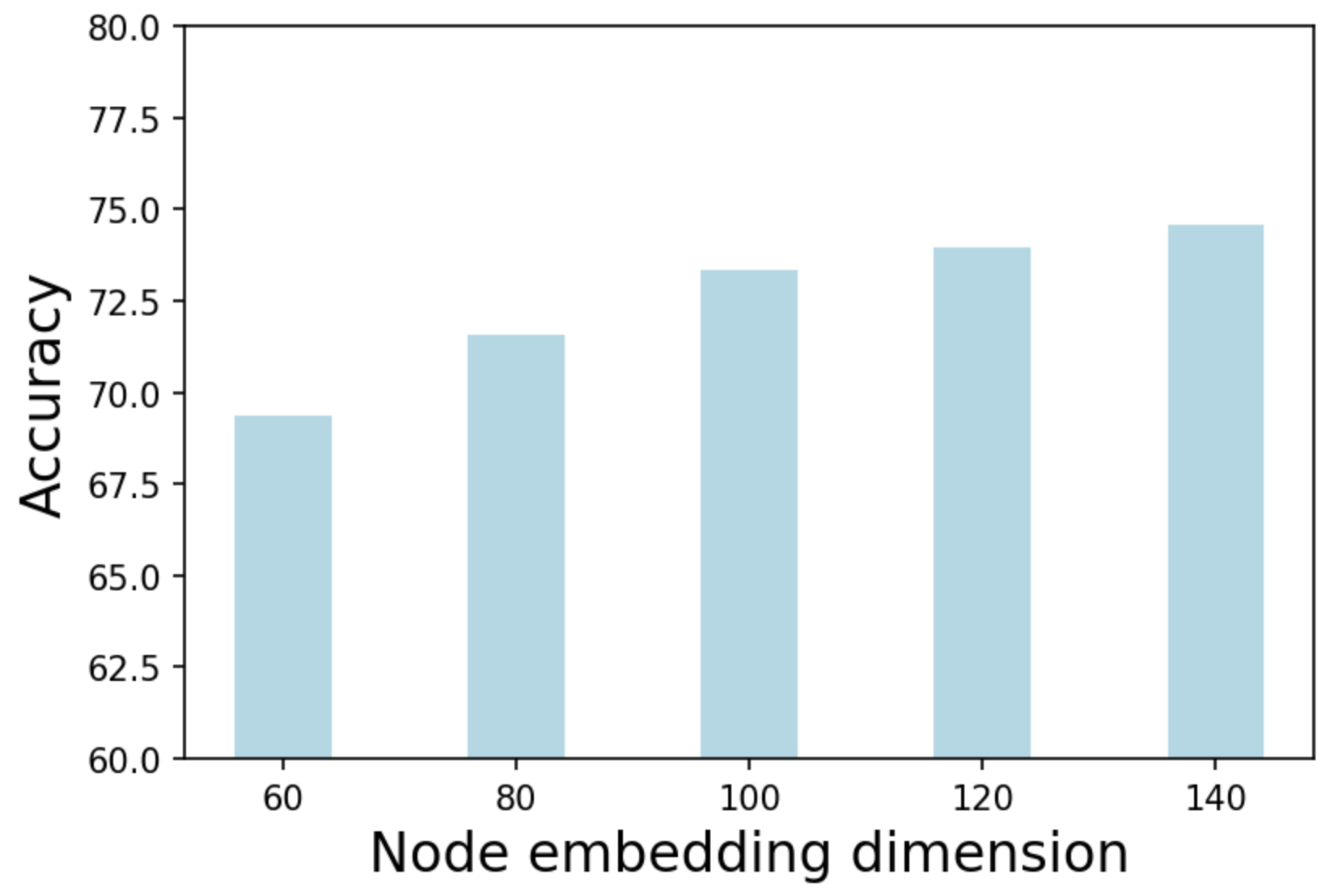
(a) Sensitivity analysis on node embeddings dimension.

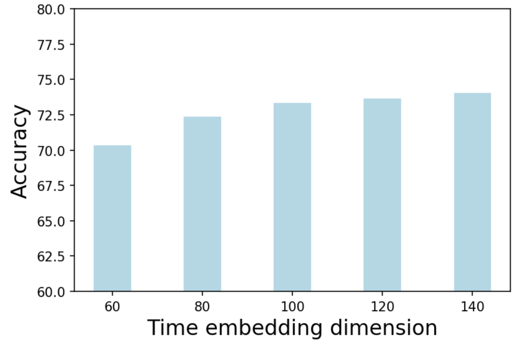
(b) Sensitivity analysis on time embeddings dimension.

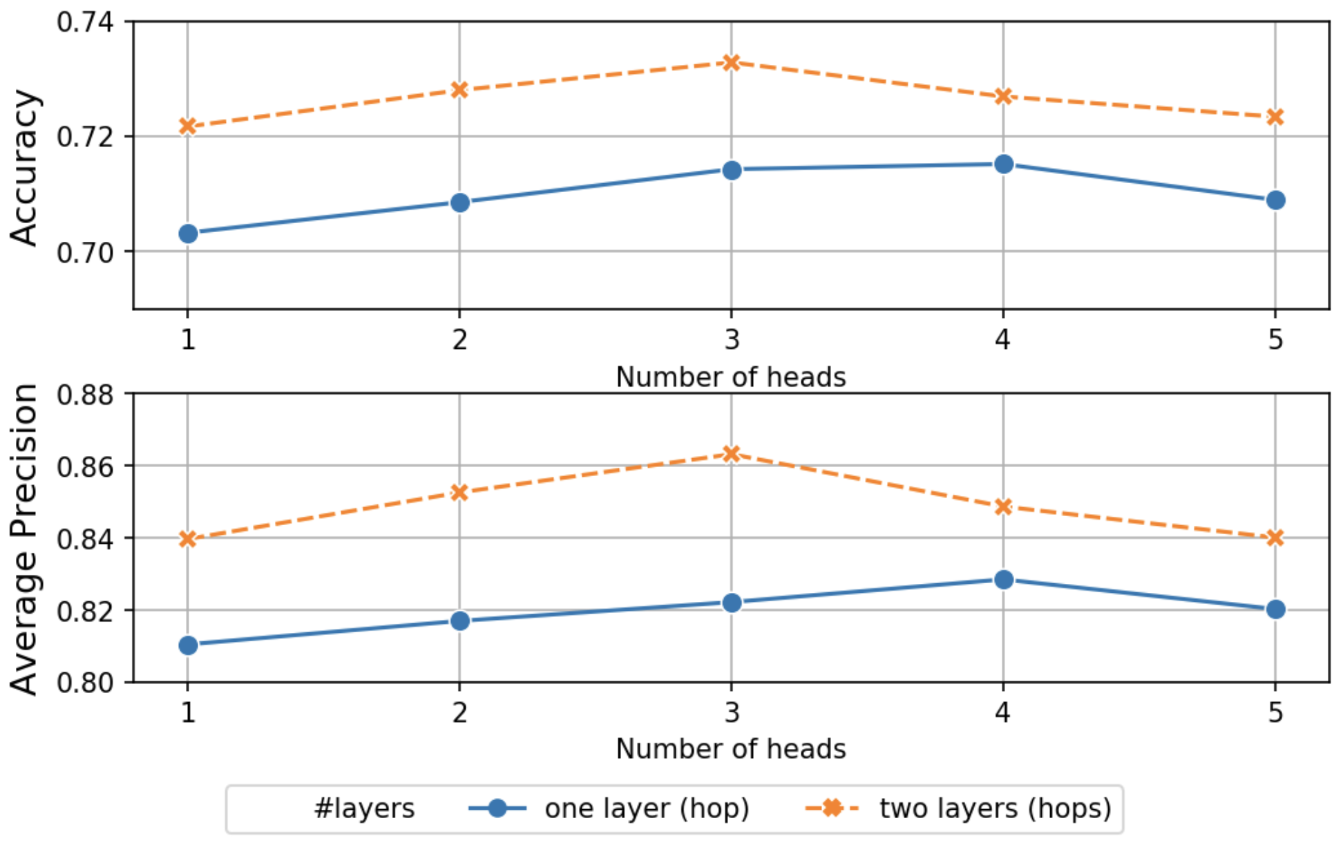
(c) Sensitivity analysis on number of attention heads and layers (hops) with $d=100$ and $d_{T}=100$.

Figure 7: Sensitivity analysis on the Industrial dataset.

Secondly, we compare between the two methods of learning functional encoding, i.e. using flow-based model or using the non-parametric method introduced in Section 3.1. We experiment on two flow-based state-of-the-art CDF learning method: normalizing flow (Rezende & Mohamed, 2015) and RealNVP (Dinh et al., 2016). We use the default model setups and hyper-parameters in their reference implementations . We provide the results in Figure 6(b). As we mentioned before, using flow-based models leads to highly comparable outcomes as the non-parametric approach, but they require longer training time since they implement sampling during each training batch. However, it is possible that carefully-tuned flow-based models can lead to nontrivial improvements, which we leave to the future work.

Finally, we provide sensitivity analysis on the number of attention heads and layers for TGAT. Recall that by stacking two layers in TGAT we are aggregating information from the two-hop neighbourhood. For both accuracy and AP, using three-head attention and two-layers gives the best outcome. In general, the results are relatively stable to the number of heads, and stacking two layers leads to significant improvements compared with using only a single layer.

The ablation study for comparing between uniform neighborhood dropout and sampling with inverse timespan is given in Figure 6(a). The two experiments are carried out under the same setting which we reported in Section 4.4. We see that using the inverse timespan sampling gives slightly worse performances. This is within expectation since uniform sampling has advantage in capturing the recurrent patterns, which can be important for predicting user actions. On the other hand, the results also suggest the effectiveness of the proposed time encoding for capturing such temporal patterns. Moreover, we point out that using the inverse timespan sampling slows down training, particularly for large graphs where a weighted sampling is conducted within a large number of nodes for each training batch construction. Nonetheless, inverse timespan sampling can help capturing the more recent interactions which may be more useful for certain tasks. Therefore, we suggest to choose the neighborhood dropout method according to the specific use cases.

References

- Bahdanau et al. (2014) Dzmitry Bahdanau, Kyunghyun Cho, and Yoshua Bengio. Neural machine translation by jointly learning to align and translate. arXiv preprint arXiv:1409.0473, 2014.
- Battaglia et al. (2018) Peter W Battaglia, Jessica B Hamrick, Victor Bapst, Alvaro Sanchez-Gonzalez, Vinicius Zambaldi, Mateusz Malinowski, Andrea Tacchetti, David Raposo, Adam Santoro, Ryan Faulkner, et al. Relational inductive biases, deep learning, and graph networks. arXiv preprint arXiv:1806.01261, 2018.
- Defferrard et al. (2016) Michaël Defferrard, Xavier Bresson, and Pierre Vandergheynst. Convolutional neural networks on graphs with fast localized spectral filtering. In Advances in neural information processing systems, pp. 3844–3852, 2016.
- Dinh et al. (2016) Laurent Dinh, Jascha Sohl-Dickstein, and Samy Bengio. Density estimation using real nvp. arXiv preprint arXiv:1605.08803, 2016.
- Fey & Lenssen (2019) Matthias Fey and Jan E. Lenssen. Fast graph representation learning with PyTorch Geometric. In ICLR Workshop on Representation Learning on Graphs and Manifolds, 2019.
- Goyal et al. (2018) Palash Goyal, Nitin Kamra, Xinran He, and Yan Liu. Dyngem: Deep embedding method for dynamic graphs. arXiv preprint arXiv:1805.11273, 2018.
- Grover & Leskovec (2016) Aditya Grover and Jure Leskovec. node2vec: Scalable feature learning for networks. In Proceedings of the 22nd ACM SIGKDD international conference on Knowledge discovery and data mining, pp. 855–864. ACM, 2016.
- Hamilton et al. (2017a) Will Hamilton, Zhitao Ying, and Jure Leskovec. Inductive representation learning on large graphs. In Advances in Neural Information Processing Systems, pp. 1024–1034, 2017a.
- Hamilton et al. (2017b) William L Hamilton, Rex Ying, and Jure Leskovec. Representation learning on graphs: Methods and applications. arXiv preprint arXiv:1709.05584, 2017b.
- Henaff et al. (2015) Mikael Henaff, Joan Bruna, and Yann LeCun. Deep convolutional networks on graph-structured data. arXiv preprint arXiv:1506.05163, 2015.
- Kingma & Welling (2013) Diederik P Kingma and Max Welling. Auto-encoding variational bayes. arXiv preprint arXiv:1312.6114, 2013.
- Kipf & Welling (2016a) Thomas N Kipf and Max Welling. Semi-supervised classification with graph convolutional networks. arXiv preprint arXiv:1609.02907, 2016a.
- Kipf & Welling (2016b) Thomas N Kipf and Max Welling. Variational graph auto-encoders. arXiv preprint arXiv:1611.07308, 2016b.
- Li et al. (2018) Taisong Li, Jiawei Zhang, S Yu Philip, Yan Zhang, and Yonghong Yan. Deep dynamic network embedding for link prediction. IEEE Access, 6:29219–29230, 2018.
- Loomis (2013) Lynn H Loomis. Introduction to abstract harmonic analysis. Courier Corporation, 2013.
- Ma et al. (2018) Yao Ma, Ziyi Guo, Eric Zhao Zhaochun Ren, and Dawei Yin Jiliang Tang. Streaming graph neural networks. arXiv preprint arXiv:1810.10627, 2018.
- Monti et al. (2017) Federico Monti, Davide Boscaini, Jonathan Masci, Emanuele Rodola, Jan Svoboda, and Michael M Bronstein. Geometric deep learning on graphs and manifolds using mixture model cnns. In Proceedings of the IEEE Conference on Computer Vision and Pattern Recognition, pp. 5115–5124, 2017.
- Nguyen et al. (2018) Giang Hoang Nguyen, John Boaz Lee, Ryan A Rossi, Nesreen K Ahmed, Eunyee Koh, and Sungchul Kim. Continuous-time dynamic network embeddings. In Companion Proceedings of the The Web Conference 2018, pp. 969–976. International World Wide Web Conferences Steering Committee, 2018.
- Pennebaker et al. (2001) James W Pennebaker, Martha E Francis, and Roger J Booth. Linguistic inquiry and word count: Liwc 2001. Mahway: Lawrence Erlbaum Associates, 71(2001):2001, 2001.
- Perozzi et al. (2014) Bryan Perozzi, Rami Al-Rfou, and Steven Skiena. Deepwalk: Online learning of social representations. In Proceedings of the 20th ACM SIGKDD international conference on Knowledge discovery and data mining, pp. 701–710. ACM, 2014.
- Rahimi & Recht (2008) Ali Rahimi and Benjamin Recht. Random features for large-scale kernel machines. In Advances in neural information processing systems, pp. 1177–1184, 2008.
- Rahman et al. (2018) Mahmudur Rahman, Tanay Kumar Saha, Mohammad Al Hasan, Kevin S Xu, and Chandan K Reddy. Dylink2vec: Effective feature representation for link prediction in dynamic networks. arXiv preprint arXiv:1804.05755, 2018.
- Rezende & Mohamed (2015) Danilo Jimenez Rezende and Shakir Mohamed. Variational inference with normalizing flows. arXiv preprint arXiv:1505.05770, 2015.
- Simonovsky & Komodakis (2017) Martin Simonovsky and Nikos Komodakis. Dynamic edge-conditioned filters in convolutional neural networks on graphs. In Proceedings of the IEEE conference on computer vision and pattern recognition, pp. 3693–3702, 2017.
- Sukhbaatar et al. (2015) Sainbayar Sukhbaatar, Jason Weston, Rob Fergus, et al. End-to-end memory networks. In Advances in neural information processing systems, pp. 2440–2448, 2015.
- Tang et al. (2015) Jian Tang, Meng Qu, Mingzhe Wang, Ming Zhang, Jun Yan, and Qiaozhu Mei. Line: Large-scale information network embedding. In Proceedings of the 24th international conference on world wide web, pp. 1067–1077. International World Wide Web Conferences Steering Committee, 2015.
- Trivedi et al. (2018) Rakshit Trivedi, Mehrdad Farajtabar, Prasenjeet Biswal, and Hongyuan Zha. Representation learning over dynamic graphs. arXiv preprint arXiv:1803.04051, 2018.
- Vaswani et al. (2017) Ashish Vaswani, Noam Shazeer, Niki Parmar, Jakob Uszkoreit, Llion Jones, Aidan N Gomez, Łukasz Kaiser, and Illia Polosukhin. Attention is all you need. In Advances in neural information processing systems, pp. 5998–6008, 2017.
- Veličković et al. (2017) Petar Veličković, Guillem Cucurull, Arantxa Casanova, Adriana Romero, Pietro Lio, and Yoshua Bengio. Graph attention networks. arXiv preprint arXiv:1710.10903, 2017.
- Wang et al. (2016) Daixin Wang, Peng Cui, and Wenwu Zhu. Structural deep network embedding. In Proceedings of the 22nd ACM SIGKDD international conference on Knowledge discovery and data mining, pp. 1225–1234. ACM, 2016.
- Wang et al. (2018a) Jizhe Wang, Pipei Huang, Huan Zhao, Zhibo Zhang, Binqiang Zhao, and Dik Lun Lee. Billion-scale commodity embedding for e-commerce recommendation in alibaba. In Proceedings of the 24th ACM SIGKDD International Conference on Knowledge Discovery & Data Mining, pp. 839–848. ACM, 2018a.
- Wang et al. (2018b) Yue Wang, Yongbin Sun, Ziwei Liu, Sanjay E Sarma, Michael M Bronstein, and Justin M Solomon. Dynamic graph cnn for learning on point clouds. arXiv preprint arXiv:1801.07829, 2018b.
- Xu et al. (2019a) Da Xu, Chuanwei Ruan, Evren Korpeoglu, Sushant Kumar, and Kannan Achan. Self-attention with functional time representation learning. In Advances in Neural Information Processing Systems, pp. 15889–15899, 2019a.
- Xu et al. (2019b) Da Xu, Chuanwei Ruan, Kamiya Motwani, Evren Korpeoglu, Sushant Kumar, and Kannan Achan. Generative graph convolutional network for growing graphs. In ICASSP 2019-2019 IEEE International Conference on Acoustics, Speech and Signal Processing (ICASSP), pp. 3167–3171. IEEE, 2019b.
- Xu et al. (2020) Da Xu, Chuanwei Ruan, Evren Korpeoglu, Sushant Kumar, and Kannan Achan. Product knowledge graph embedding for e-commerce. In Proceedings of the 13th International Conference on Web Search and Data Mining, pp. 672–680, 2020.
- Ying et al. (2018) Rex Ying, Ruining He, Kaifeng Chen, Pong Eksombatchai, William L Hamilton, and Jure Leskovec. Graph convolutional neural networks for web-scale recommender systems. In Proceedings of the 24th ACM SIGKDD International Conference on Knowledge Discovery & Data Mining, pp. 974–983. ACM, 2018.