Sum-Product Optimization via Relational Equality Saturation for Large Scale Linear Algebra

SPORES: Sum-Product Optimization via Relational Equality Saturation for Large Scale Linear Algebra

Abstract

Machine learning algorithms are commonly specified in linear algebra (LA). LA expressions can be rewritten into more efficient forms, by taking advantage of input properties such as sparsity, as well as program properties such as common subexpressions and fusible operators. The complex interaction among these properties’ impact on the execution cost poses a challenge to optimizing compilers. Existing compilers resort to intricate heuristics that complicate the codebase and add maintenance cost but fail to search through the large space of equivalent LA expressions to find the cheapest one. We introduce a general optimization technique for LA expressions, by converting the LA expressions into Relational Algebra (RA) expressions, optimizing the latter, then converting the result back to (optimized) LA expressions. One major advantage of this method is that it is complete, meaning that any equivalent LA expression can be found using the equivalence rules in RA. The challenge is the major size of the search space, and we address this by adopting and extending a technique used in compilers, called equality saturation. We integrate the optimizer into SystemML and validate it empirically across a spectrum of machine learning tasks; we show that we can derive all existing hand-coded optimizations in SystemML, and perform new optimizations that lead to speedups from $1.2X$ to $5X$.

1 Introduction

Consider the Linear Algebra (LA) expression $sum((X-UV^{T})^{2})$ which defines a typical loss function for approximating a matrix $X$ with a low-rank matrix $UV^{T}$. Here, $sum()$ computes the sum of all matrix entries in its argument, and $A^{2}$ squares the matrix $A$ element-wise. Suppose $X$ is a sparse, 1M x 500k matrix, and suppose $U$ and $V$ are dense vectors of dimensions 1M and 500k respectively. Thus, $UV^{T}$ is a rank 1 matrix of size 1M x 500k, and computing it naively requires 0.5 trillion multiplications, plus memory allocation. Fortunately, the expression is equivalent to $sum(X^{2})-2U^{T}XV+U^{T}U*V^{T}V$. Here $U^{T}XV$ is a scalar that can be computed efficiently by taking advantage of the sparsity of $X$, and, similarly, $U^{T}U$ and $V^{T}V$ are scalar values requiring only 1M and 500k multiplications respectively.

Optimization opportunities like this are ubiquitous in machine learning programs. State-of-the-art optimizing compilers such as SystemML [1], OptiML[27], and Cumulon[11] commonly implement syntactic rewrite rules that exploit the algebraic properties of the LA expressions. For example, SystemML includes a rule that rewrites the preceding example to a specialized operator to compute the result in a streaming fashion. However, such syntactic rules fail on the simplest variations, for example SystemML fails to optimize $sum((X+UV^{T})^{2})$, where we just replaced $-$ with $+$. Moreover, rules may interact with each other in complex ways. In addition, complex ML programs often have many common subexpressions (CSE), that further interact with syntactic rules, for example the same expression $UV^{T}$ may occur in multiple contexts, each requiring different optimization rules.

In this paper we describe SPORES, a novel optimization approach for complex linear algebra programs that leverages relational algebra as an intermediate representation to completely represent the search space. SPORES first transforms LA expressions into traditional Relational Algebra (RA) expressions consisting of joins $*$, union $+$ and aggregates $\sum$. It then performs a cost-based optimizations on the resulting Relational Algebra expressions, using only standard identities in RA. Finally, the resulting RA expression is converted back to LA, and executed.

A major advantage of SPORES is that the optimization rules in RA are complete. Linear Algebra seems to require an endless supply of clever rewrite rules, but, in contrast, by converting to RA, we can prove that SPORES is complete. The RA expressions in this paper are over $K$-relations [9]; a tuple $X(i,j)$ is no longer true or false, but has a numerical value, e.g. $5$; in other words, the RA expressions that result from LA expressions are interpreted over bags instead of sets. A folklore theorem states that two Unions of Conjunctive Queries over bag semantics are equivalent iff they are isomorphic, which implies that checking equivalence is decidable. (In contrast, containment of two UCQs with bag semantics is undecidable [13]; we do not consider containment in this paper.) We prove that our optimizer rules are sufficient to convert any RA expression into its canonical form, i.e. to an UCQ, and thus can, in principle, can discover all equivalent rewritings.

However, we faced a major challenge in trying to exploit the completeness of the optimizer. The search space is very large, typically larger than that encountered in standard database optimizers, because of the prevalence of unions $+$, large number of aggregates $\sum$, and frequent common subexpressions. To tackle this, SPORES adopts and extends a technique from compilers called equality saturation [28]. It uses a data structure called the E-Graph [22] to compactly represent the space of equivalent expressions, and equality rules to populate the E-Graph, then leverages constraint solvers to extract the optimal expression from the E-Graph.

We have integrated SPORES into SystemML [1], and show that it can derive all hand-coded rules of SystemML. We evaluated SPORES on a spectrum of machine learning tasks, showing competitive performance improvement compared with more mature heuristic-based optimizers. Our optimizer rediscovers all optimizations by the latter, and also finds new optimizations that contribute to speedups of 1.2X to 5X.

We make the following contributions in this paper:

1. We describe a novel approach for optimizing complex Linear Algebra expressions by converting them to Relational Algebra, and prove that this approach is complete (Sec. 2).

2. We present search algorithm based on Equality Saturation that can explore a large search space while reusing memory (Sec. 3).

3. We conduct an empirical evaluation of the optimizer using several real-world machine learning tasks, and demonstrate it’s superiority over an heuristics-driven optimizer in SystemML (Sec. 4).

2 Representing the Search Space

2.1 Rules $R_{LR}$: from LA to RA and Back

In this section we describe our approach of optimizing LA expressions by converting them to RA. The rules converting from LA to RA and back are denoted $R_{LR}$.

To justify our approach, let us revisit our example loss function written in LA and attempt to optimize it using standard LA identities. Here we focus on algebraic rewrites and put aside concerns about the cost model. Using the usual identities on linear algebra expressions, one may attempt to rewrite the original expression as follows:

$$sum((X-UV^{T})^{2})$$

$$= sum((X-UV^{T})*(X-UV^{T}))$$

$$= sum(X^{2}-2X*UV^{T}+(UV^{T})^{2})$$

$$= sum(X^{2})-2sum(X*UV^{T})+sum((UV^{T})^{2})$$

At this point we are stuck trying to rewrite $sum(X*UV^{T})$ (recall that $*$ is element-wise multiplication); it turns out to be equal to $sum(U^{T}XV)$, for any matrices $X,U,V$ (and it is equal to the scalar $U^{T}XV$ when $U,V$ are column vectors), but this does not seem to follow from standard LA identities like associativity, commutativity, and distributivity. Similarly, we are stuck trying to rewrite $sum((UV^{T})^{2})$ to $sum(U^{T}U*V^{T}V)$. Current systems manually add syntactic rewrite rules, whenever such a special case is deemed frequent enough to justify extending the optimizer.

	$A$	$x$	$A*x^{T}$	$Ax$
LA:	$\begin{bmatrix}0&5\\ 7&0\end{bmatrix}$	$\begin{bmatrix}3\\ 2\end{bmatrix}$	$\begin{bmatrix}0&10\\ 21&0\end{bmatrix}$	$\begin{bmatrix}10\\ 21\end{bmatrix}$
RA:	$i$ $j$ # $1$ $2$ 5 $2$ $1$ 7	$j$ # 1 3 2 2	$i$ $j$ # $1$ $2$ 10 $2$ $1$ 21	$i$ # 1 10 2 21

Figure 1: Top: Linear Algebra manipulates matrices and vectors. $A*x^{T}$ is element-wise multiplication, computing the matrix $(A_{ij}x_{j})_{ij}$, while $Ax$ is standard matrix-vector multiplication. Bottom: their translations into $K$-relations and Relational Algebra operations. Each relation is a bag, where the attribute $\#$ represents the multiplicity, i.e. $A(1,2)$ has multiplicity $5$ etc. Then $A*x^{T}$ becomes a standard query $Q(i,j)=A(i,j)*x(j)$, while $Ax$ is a query with a group-by and aggregate, $Q(i)=\sum_{j}A(i,j)*x(j)$.

Instead, our approach is to expand out the LA expression element-wise. For example, assuming for simplicity that $U,V$ are column vectors, we obtain

$$sum((UV^{T})^{2})=\textstyle{\sum_{i,j}}(U_{i}*V_{j})*(U_{i}*V_{j})$$

$$=\textstyle{\sum_{i,j}}(U_{i}*U_{i})*(V_{j}*V_{J})$$

$$=(\textstyle{\sum_{i}}U_{i}*U_{i})*(\textstyle{\sum_{j}}V_{j}*V_{j})$$

$$=U^{T}U*V^{T}V$$

The expressions using indices represent Relational Algebra expressions. More precisely, we interpret every vector, or matrix, or tensor, as a $K$-relation [9] over the reals. In other words we view $X_{ij}$ is a tuple $X(i,j)$ whose “multiplicity” is the real value of that matrix element. We interpret point-wise multiply as natural join; addition as union; sum as aggregate; and matrix multiply as aggregate over a join. Figure 1 illustrates the correspondence between LA and RA. We treat each matrix entry $A_{ij}$ as the multiplicity of tuple $(i,j)$ in relation $A$ under bag semantics. For example $A_{2,1}=7$, therefore the tuple $(2,1)$ has multiplicity of $7$ in the corresponding relation. $A*x^{T}$ denotes element-wise multiplication, where each element $A_{ij}$ of the matrix is multiplied with the element $x_{j}$ of the row-vector $x^{T}$. In RA it is naturally interpreted as the natural join $A(i,j)\Join x(j)$, which we write as $A(i,j)*x(j)$. Similarly, $Ax$ is the standard matrix-vector multiplication in LA, while in RA it becomes a query with a group by and aggregate, which we write as $\sum_{j}A(i,j)*x(j)$. Our $K$-relations are more general than bags, since the entry of a matrix can be a real number, or a negative number; they correspond to $K$-relations over the semiring of reals $(\mathbb{R},0,1,+,*)$.

	name	type	syntax
LA	mmult	$M_{M,L}\times M_{L,N}\rightarrow M_{M,N}$	$AB$ or MxM
	elemmult	$M_{M,N}\times M_{M,N}\rightarrow M_{M,N}$	$A*B$
	elemplus	$M_{M,N}\times M_{M,N}\rightarrow M_{M,N}$	$A+B$
	rowagg	$M_{M,N}\rightarrow M_{M,1}$	$sum_{row}A$
	colagg	$M_{M,N}\rightarrow M_{1,N}$	$sum_{col}A$
	agg	$M_{M,N}\rightarrow M_{1,1}$	$sumA$
	transpose	$M_{M,N}\rightarrow M_{N,M}$	$A^{\mathsf{T}}$
conv.	bind	$M_{M,N}\times[i,j]\rightarrow R_{i:M,j:N}$	${\scriptstyle\left[i,j\right]\,}A$
	unbind	$R_{i:M,j:N}\times[i,j]\rightarrow M_{M,N}$	${\scriptstyle\left[-i,-j\right]\,}A$
RA	join	$R_{S_{1}}\times R_{S_{2}}\rightarrow R_{S_{1}\cup S_{2}}$	$A*B$
	union	$R_{S_{1}}\times R_{S_{2}}\rightarrow R_{S_{1}\cup S_{2}}$	$A+B$
	agg	$R_{S}\times U\rightarrow R_{S\setminus U}$	$\sum_{U}A$

Table 1: LA and RA Operators. The type $M_{M,N}$ is a matrix of size $M\times N$; $[i,j]$ is a list of attribute names; $R_{i:M,j:N}$ is a relation with attributes $i$ of size $M$ and $j$ of size $N$; $S_{1},S_{2},S,$ and $U$ are sets of attributes.

1. $A*B\rightarrow{\scriptstyle\left[-i,-j\right]\,}({\scriptstyle\left[i,j\right]\,}A*{\scriptstyle\left[i,j\right]\,}B)$.

2. $A+B\rightarrow{\scriptstyle\left[-i,-j\right]\,}({\scriptstyle\left[i,j\right]\,}A+{\scriptstyle\left[i,j\right]\,}B)$.

3. $sum_{row}A\rightarrow[-i,\_]\sum_{j}{\scriptstyle\left[i,j\right]\,}A$. Similar for $sum_{col}$, $sum$.

4. $AB\rightarrow{\scriptstyle\left[-i,-k\right]\,}\sum_{j}({\scriptstyle\left[i,j\right]\,}A*{\scriptstyle\left[j,k\right]\,}B)$.

5. $A^{\mathsf{T}}\rightarrow{\scriptstyle\left[-j,-i\right]\,}{\scriptstyle\left[i,j\right]\,}A$.

6. $A-B\rightarrow A+(-1)*B$

Figure 2: LA-to-RA Ruleset $R_{LR}$. Notice that $*$ means point-wise multiply for matrices, but means natural join for relations. Similarly, $+$ means addition for matrices, but union for relations.

We now describe the general approach in SPORES. The formal definition of LA and RA are in Table 1. LA consists of seven operators, which are those supported in SystemML [1]. RA consists of only three operators: $*$ (natural join), $+$ (union), and $\sum$ (group-by aggregate). Difference is represented as $A-B=A+(-1)B$ (this is difference in $\mathbb{R}$; we do not support bag difference, i.e. difference in $\mathbb{N}$ like $3-5=0$, because there is no corresponding operation in LA), while selection can be encoded by multiplication with relations with 0/1 entries. We call an expression using these three RA operators an RPlan, for Relational Plan, and use the terms RPlan and RA/relational algebra interchangeably. Finally, there are two operators, bind and unbind for converting between matrices/vectors and $K$-relations.

The translation from LA to RA is achieved by a set of rules, denoted $R_{LR}$, and shown in Figure 2. The bind operator ${\scriptstyle\left[i,j\right]\,}$ converts a matrix to a relation by giving attributes $i,j$ to its two dimensions; the unbind operator ${\scriptstyle\left[-i,-j\right]\,}$ converts a relation back to a matrix. For example, ${\scriptstyle\left[-j,-i\right]\,}{\scriptstyle\left[i,j\right]\,}A$ binds $A$’s row indices to $i$ and its column indices to $j$, then unbinds them in the opposite order, thereby transposing $A$.

SPORES translates a complex LA expression into RA by first applying the rules $R_{LR}$ in Figure 2 to each LA operator, replacing it with an RA operator, preceded by bind and followed by unbind. Next, it eliminates consecutive unbind/bind operators, possibly renaming attributes, e.g. ${\scriptstyle\left[k,l\right]\,}{\scriptstyle\left[-i,-j\right]\,}A$ becomes $A[i\to k,j\to l]$, which indicates that the attributes $i$ and $j$ in $A$’s schema should be renamed to $k$ and $l$, by propagating the rename downward into $A$. As a result, the entire LA expression becomes an RA expression (RPlan), with bind operators on the leaves, and unbind at the top. For an illustration, the left DAG in Figure 6 shows the expression $sum((X-UV^{T})^{2})$ translated to relational algebra.

1. $A*(B+C)=A*B+A*C$

2. $\sum_{i}(A+B)=\sum_{i}A+\sum_{i}B$

3. If $i\not\in A$, $A*\sum_{i}B=\sum_{i}(A*B)\quad$ (else rename $i$)

4. $\sum_{i}\sum_{j}A=\sum_{i,j}A$

5. If $i\not\in Attr(A)$, then $\sum_{i}A=A*dim(i)$

6. $A+(B+C)=+(A,B,C)\quad$ (assoc. & comm.)

7. $A*(B*C)=*(A,B,C)\quad$ (assoc. & comm.)

Figure 3: RA equality rules $R_{EQ}$. $*$ means natural join and $+$ means union.

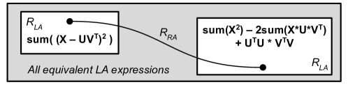
Figure 4: Venn diagram of LA and/or RA expressions. Each of the two white islands represent LA expressions that can be proven equivalent using identities in LA; there is no way to move from one island to the other by using LA identities. The large gray box shows the set of expressions that can be proven equivalent by using RA identities. This allows us to connect the two islands.

Figure 5: Two LA expressions $e_{LA}$ and $e^{\prime}_{LA}$ are equivalent iff their relational counterparts $e_{RA}$ and $e^{\prime}_{RA}$ have isomorphic canonical forms $\mathcal{C}(e_{RA}),\mathcal{C}(e^{\prime}_{RA})$. $R_{LR}$ translates a LA expression to RA and $R_{EQ}$ are the relational equality rules.

Figure 6: RA DAGs for $sum((X-UV^{T})^{2})$ (left) and its canonical form (right).

2.2 Rules $R_{EQ}$ : from RA to RA

The equational rules for RA consists of seven identities shown in Figure 3, and denoted by $R_{EQ}$. The seven rules are natural relational algebra identities, where $*$ corresponds to natural join, $+$ to union (of relations with the same schema) and $\sum_{i}$ to group-by and aggregate. In rule 5, $i\notin Attr(A)$ means that $i$ is not an attribute of $A$, and $dim(i)$ is the dimension of index $i$. For a very simple illustration of this rule, consider $\sum_{i}5$. Here $5$ is a constant, i.e. a relation of zero arity, with no attributes. The rule rewrites it to $5dim(i)$, where $dim(i)$ is a number representing the dimension of $i$.

2.3 Completeness of the Optimization Rules

As we have seen at the beginning of this section, when rewriting LA expressions using identities in linear algebra we may get stuck. This is illustrated in Figure 4, which shows two white islands representing sets of provably equivalent LA expressions; the simple identities in LA allow us to move within one white island, but are insufficient to move from one island to the other. Instead, by rewriting the expressions to RA, the seven identities in $R_{EQ}$ are much more powerful, and allow us to prove them equivalent. We prove here that this approach is complete, meaning that, if two LA expressions are semantically equivalent, then their equivalence can be proven by using rules $R_{EQ}$. The proof consists of two parts: (1) the rules $R_{EQ}$ are sufficient to convert any RA expression $e$ to its normal form (also called canonical form) $\mathcal{C}(e)$, and back, (2) two RA expressions $e,e^{\prime}$ are semantically equal iff they have isomorphic normal forms, $\mathcal{C}(e)\equiv\mathcal{C}(e^{\prime})$. Figure 5 shows the main steps at a high level: two LA expressions are semantically equivalent if and only if their canonical form in RA are isomorphic, where $R_{LR}$ translates each expression to RA and $R_{EQ}$ takes the RA expression to its canonical form. Throughout this section we write $e\ R_{EQ}^{*}\ e^{\prime}$ when $e,e^{\prime}$ can be proven equal by using the identities in $R_{EQ}$ (Fig. 3).

Normal Form The normal form of an RPlan is similar in spirit to the canonical form of polynomials as a sum of monomials, except that the monomial terms also include aggregations. As for polynomials, we combine equal factors by introducing power, e.g. $X*X$ becomes $X^{2}$, and combine isomorphic monomials by introducing constant coefficients, e.g. $3X^{2}Y+5X^{2}Y$ becomes $8X^{2}Y$. For example, the following RPlan denotes a 1-dimensional vector $Q(i)=(\sum_{j}x(i,j)*(\sum_{k}y(j,k)*x(i,j))+\sum_{m,n}x(i,m)^{2}y(m,n)$ and its canonical form is $2\sum_{j,k}x(i,j)^{2}y(j,k)$. Formally:

Definition 2.1.

An RA expression is canonical, or in normal form, if it is the sum (i.e. $+$) of $n$ monomials, where each monomial $i$ consists of a constant $c_{i}$ multiplied by an aggregation over a (possibly empty) set of attributes $A_{i}$ (for $1\leq i\leq n$), of a product of $m_{i}$ factors, where each factor is some matrix or vector $x_{ij}$ (for $1\leq i\leq n$, $1\leq j\leq m_{i}$) indexed by some index variables (not shown), and possibly raised to some power:

$$c_{1}\sum_{A_{1}}\left(x_{11}^{k_{11}}*\dots*x_{1m_{1}}^{k_{1m_{1}}}\right)+\dots+c_{n}\sum_{A_{n}}\left(x_{n1}^{k_{n1}}*\dots*x_{nm_{n}}^{k_{nm_{n}}}\right)$$

We further assume that no monomial contains the same factor twice (otherwise, replace it with a single factor with a higher power $k_{ij}$) and no two monomials are isomorphic (otherwise we replace them with a single monomial with a larger coefficient $c_{i}$)

The order of summands and multiplicands is insignificant because $*$ and $+$ are commutative and associative. We notice that, unlike traditional polynomials, here the same matrix name may occur in different factors, for example in $\sum_{i,j,k}x(i,j)*x(j,k)*x(k,i)$ the matrix $x$ occurs three times, but the factors are different i.e. we cannot write $x^{3}$.

The first of the completeness proof consists in showing that every expression $e$ in RA is equivalent to some normal form $\mathcal{C}(e)$, and, moreover, that their equivalence can be proven using the rules $R_{EQ}$ in Figure 3.

Lemma 2.1.

$\forall e\in RA$ there exists a canonical form $\mathcal{C}(e)$ and, moreover, their equivalence follows from the rules in $R_{EQ}$, in notation: $e\ R_{EQ}^{*}\ \mathcal{C}(e)$.

The proof is a straightforward induction on the structure of $e$. We apply distributivity of $*$ over $+$, then pull out the summation $\sum$; we omit the details. We illustrate in Figure 6 the canonical form of the expression $sum((X-UV^{T})^{2})$. Notice that, since the rules in $R_{EQ}$ are sound, it follows that any expression $e$ has the same semantics as its canonical form $\mathit{C}(e)$.

The second step of the completeness proof is to show that canonical forms are unique up to isomorphism.

Lemma 2.2.

(Uniqueness of RA Normal Form) Let $e_{1},e_{2}$ be two RA expressions in normal form. Suppose that they have the same semantics, i.e. $e_{1}=e_{2}$ for all inputs with arbitrary dimensions. Then their canonical forms are isomorphic.

We give a proof of this lemma in the appendix. Here, we comment on a subtle issue, namely the requirement that $e_{1}=e_{2}$ on inputs of any dimensions is necessary. For example, if we restrict the matrices $x,y$ to be of dimension $1\times 1$, then the expressions $\sum_{i,j}x(i,j)*y(i,j)$ and $\sum_{i,j}x(i,j)*y(j,i)$ have the same semantics, but different canonical form. For another example, consider three vectors $x,y,z$ of dimension $N$. Then, if $N\leq 2$ these two expressions are identical: $\sum_{i,j,k}x(i)*y(j)*z(k)+2\sum_{i}x(i)*y(i)*z(i)$ and $\sum_{i,j}x(i)*y(i)*z(j)+\sum_{i,j}x(i)*y(j)*z(i)+\sum_{i,j}x(j)*y(i)*z(i)$, although they are not equal in general.

We are now ready to establish the completeness of RA equalities, by showing any equivalent LA expressions can be rewritten to each other through the translation rules $R_{LR}$ and the canonicalization rules $R_{EQ}$:

Theorem 2.3.

(Completeness of $R_{EQ}$) Two LA expressions are semantically equivalent if and only if their relational form is in the transitive closure of $R_{EQ}$ rules:

$$\forall e_{1},e_{2}\in\textsc{LA}{},\,\forall d.e_{1}(d)=e_{2}(d)\iff R_{LR}(e_{1})R_{EQ}^{*}R_{LR}(e_{2})$$

Here $R_{LR}(e)$ translates LA expression $e$ into RA.

Proof.

Translating $e_{1}$ and $e_{2}$ to RA preserves semantics under $R_{LR}$. By Lemma 2.1 normalizing $R_{LR}(e_{1})$ and $R_{LR}(e_{2})$ preserves semantics. By the uniqueness of the normal form (Lemma 2.2)

$$\mathcal{C}(R_{LR}(e_{1}))\equiv\mathcal{C}(R_{LR}(e_{2}))\iff R_{LR}(e_{1})=R_{LR}(e_{2})$$

Since every rule in $R_{EQ}$ is reversible,

$$R_{LR}(e_{1})=R_{LR}(e_{2})\iff R_{LR}(e_{1})R_{EQ}^{*}R_{LR}(e_{2})$$

∎

3 Exploring the Search Space

With a complete representation of the search space by relational algebra, our next step is to explore this space and find the optimal expression in it. Traditional optimizing compilers commonly resort to heuristics to select from available rewrites to apply. SystemML implements a number of heuristics for its algebraic rewrite rules, and we discuss a few categories of them here.

Competing or Conflicting Rewrites The same expression may be eligible for more than one rewrites. For example, $sum(AB)$ rewrites to $sum(sum_{col}(A)^{T}*sum_{row}(B))$, but when both $A$ and $B$ are vectors the expression can also be rewritten to a single dot product. SystemML then implements heuristics to only perform the first rewrite when the expression is not a dot product. In the worst case, a set of rules interacting with each other may create a quadratic number of such conflicts, complicating the codebase.

Order of Rewrites Some rewrite should be applied after others to be effective. For example, $X/y$ could be rewritten to $X*1/y$ which may be more efficient, since SystemML provides efficient implementation for sparse multiplication but not for division. This rewrite should occur before constant folding; otherwise it may create spurious expressions like $X/(1/y)\rightarrow X*(1/(1/y))$, and without constant folding the double division will persist. However, a rewrite like $1/(1+exp(-X))\rightarrow sigmoid(X)$ should come after constant folding, in order to cover expressions like $(3-2)/(1+exp(-X))$. Since SystemML requires all rewrites to happen in one phase and constant folding another, it has to leave out rewrites like $X/y\rightarrow X*1/y$.

Dependency on Input / Program Properties Our example optimization from $sum((X-UV^{T})^{2})$ to $sum(X^{2})-2U^{T}XV+U^{T}U*V^{T}V$ improves performance only if $X$ is sparse. Otherwise, computing $X^{2}$ and $X*UV^{T}$ would both create dense intermediates. Similarly, some rewrites depend on program properties like common subexpressions. Usually, these rewrites only apply when the matched expression shares no CSE with others in order to leverage common subexpression elimination. Testing input and program properties like this becomes boilerplate code, making implementation tedious and adds burden to maintenance.

Composing Rewrites Even more relevant to us is the problem of composing larger rewrites out of smaller ones. Our equality rules $R_{EQ}$ are very fine-grained, and any rule is unlikely to improve performance on its own. Our example optimization from $sum((X-UV^{T})^{2})$ to $sum(X^{2})-2U^{T}XV+U^{T}U*V^{T}V$ takes around 10 applications of $R_{EQ}$ rules. If an optimizer applies rewrites one by one, it is then very difficult, if not impossible, for it to discover the correct sequence of rewrites that compose together and lead to the best performance.

Stepping back, the challenge of orchestrating rewrites is known as the phase-ordering problem in compiler optimization. Tate et al. [28] proposed a solution to this problem dubbed equality saturation, which we adapt and extend in SPORES.

3.1 Equality Saturation

Equality saturation optimizes an expression in two steps:

Saturation: given the input expression, the optimizer enumerates equivalent expressions and collects them into a compact representation called the E-Graph [22].

Extraction: given a cost function, the optimizer selects the optimal expression from the E-Graph. An expression is represented by a subgraph of the E-Graph, and the optimizer uses a constraint solver to find the subgraph that is equivalent to the input, and is optimal according to the cost function.

The E-Graph Data Structure

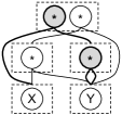
Figure 7: E-Graph representing $(X*Y)*Y$ (left), and the graph after applying associativity to the root (right). New nodes are in gray. Each dashed box is an E-Class.

An E-Graph represents sets of equivalent expressions. A node in the graph is called an E-Class, which contains the root operators of a set of equivalent expressions. The edges are similar to the edges in an abstract syntax tree; but instead of pointing from an operator directly to a child, each edge points from an operator to an E-Class of expressions. For example, in Figure 7 the top class in the middle represents the set of equivalent expressions {$(X*Y)*Y,X*(Y*Y)$}. Note that the class represents two expressions, each with 2 appearances of $Y$ and one appearance of $X$, whereas each variable only appears once in the E-Graph. This is because the E-Graph makes sure its expressions share all possible common subexpressions. As the size of the graph grows, this compression becomes more and more notable; in some cases a graph can represent a number of expressions exponential to its size [28]. We take advantage of this compression in SPORES to efficiently cover vast portions of the search space. If saturation, as described below, carries out to convergence, the E-Graph represents the search space exhaustively.

An E-Graph can also be seen as an AND-OR DAG over expressions. Each E-Class is an OR node whose children are equivalent expressions from which the optimizer chooses from. Each operator is an AND node whose children must all be picked if the operator itself is picked. In this paper we favor the terms E-Graph and E-Class to emphasize each OR node is an equivalence class.

Saturating the E-Graph

At the beginning of the optimization process, the optimizer instantiates the graph by inserting the nodes in the syntax tree of the input expression one by one in post order. For example, for input $(X*Y)*Y$, we construct the left graph in Figure 7 bottom-up. By inserting in post order, we readily exploit existing common subexpressions in the input. Once the entire input expression is inserted, the optimizer starts to extend the graph with new expressions equivalent to the input. It considers a list of equations, and matches either side of the equation to subgraphs of the E-Graph. If an equation matches, the optimizer then inserts the expression on the other side of the equation to the graph. For example, applying the associative rule extends the left graph in Figure 7 with $X*(Y*Y)$, resulting in the right graph. Figure 8 shows the pseudo code for this process. While inserting new expressions, the optimizer checks if any subexpression of the new expression is already in the graph. If so, it reuses the existing node, thereby exploiting all possible common-subexpressions to keep the E-Graph compact. In Figure 7, only two $*$ are added since the variables $X$ and $Y$ are already in the graph. Once the entire new expression has been added, the optimizer then merges the newly created E-Class at its root with the E-Class containing the matched expression, asserting them equal. Importantly, the optimizer also propagates the congruent closure of this new equality. For example, when $A+A$ is merged with $2*A$, the optimizer also merges $(A+A)^{2}$ with $(2*A)^{2}$. Figure 9 shows the pseudo code for adding an expression to E-Graph. This process of match-and-insert is repeated until the graph stops changing, or reaching a user-specified bound on the number of saturation iterations. If this process does converge, that means no rule can add new expressions to the graph any more. If the set of rules are complete, as is our $R_{EQ}$, convergence of saturation implies the resulting E-Graph represents the transitive closure of the equality rules applied to the initial expression. In other words, it contains all expressions equivalent to the input under the equality rules.

⬇

1def saturate(egraph, equations):

2 for eq in equations:

3 matches = egraph.match(eq.lhs)

4 for eclass in matches:

5 ec = egraph.add(eq.rhs)

6 egraph.merge(eclass, c)

Figure 8: Pseudo code for saturating the E-Graph given a set of equalities. match returns the IDs of the root class of any matching subgraph; merge combines two E-Classes given their IDs; it also propagates the congruent closure of the new equality. Figure 9 defines add.

⬇

1def add(expr):

2 ID = egraph.find(expr)

3 if ID != NULL:

4 return ID

5 else:

6 cids = expr.children.map(add)

7 ID = egraph.insert(expr.op, cids)

8 return ID

Figure 9: Pseudo code for adding an expression to the E-Graph. find looks for the given expression in the E-Graph, and returns its root ID if it already exists, or NULL otherwise. insert adds the given operator to the E-Graph, and points its children to E-Classes with the given class IDs.

The outer loop that matches equations to the graph can be implemented by a more efficient algorithm like the Rete algorithm [6] when the number of equations is large. However, we did not find matching to be expensive and simply match by traversing the graph. Our implementation uses the E-Graph data structure from the egg [30] library.

Dealing with Expansive Rules

While in theory equality saturation will converge with well-constructed rewrite rules, in practice the E-Graph may explode for certain inputs under certain rules. For example, a long chain of multiplication can be rewritten to an exponential number of permutations under associativity and commutativity (AC rules). If we apply AC rules everywhere applicable in each iteration, the graph would soon use up available memory. We call this application strategy the depth-first strategy because it eagerly applies expansive rules like AC. AC rules by themselves rarely affect performance, and SystemML also provides the fused mmchain operator that efficiently computes multiplication chains, so permuting a chain is likely futile. In practice, AC rules are useful because they can enable other rewrites. Suppose we have a rule $R_{factor}:A*X+B*X\rightarrow(A+B)*X$ and an expression $U*Y+Y*V$. Applying commutativity to $Y*V$ would then transform the expression to be eligible for $R_{factor}$. With this insight, we change each saturation iteration to sample a limited number of matches to apply per rule, instead of applying all matches. This amounts to adding matches = sample(matches, limit) between line 3 and line 4 in Figure 9. Sampling encourages each rule to be considered equally often and prevents any single rule from exploding the graph. This helps ensure good exploration of the search space when exhaustive search is impractical. But when it is possible for saturation to converge and be exhaustive, it still converges with high probability when we sample matches. Our experiments in Section 4.3 show sampling always preserve convergence in practice.

Extracting the Optimal Plan

Figure 10: The CSE problem. Each node shows its cost. A greedy optimizer picks nodes with costs 0, 1 and both nodes with cost 4; but the optimal plan uses nodes with costs 0, 2 and shares the same node with cost 4.

A greedy strategy to extract the best plan from the saturated E-Graph is to traverse the graph bottom-up, picking the best plan at each level. This assumes the best plan for any expression also contains the best plan for any of its subexpressions. However, the presence of common subexpressions breaks this assumption. In Figure 10 each operator node is annotated with its cost. Between the nodes with costs 1 and 2, a greedy strategy would choose 1, which incurs total cost of $1+4=5$. The greedy strategy then needs to pick the root node with cost 0 and the other node with cost 4, incurring a total cost of 9. However, the optimal strategy is to pick the nodes with 0, 2 and share the same node with cost 4, incurring a total cost of 6.

We handle the complexity of the search problem with a constraint solver. We assign a variable to each operator and each E-Class, then construct constraints over the variables for the solver to select operators that make up a valid expression. The solver will then optimize a cost function defined over the variables; the solution then corresponds to the optimal expression equivalent to the input.

Constraint Solving and Cost Function

We encode the problem of extracting the cheapest plan from the E-Graph with integer linear programming (ILP). Figure 11 shows this encoding. For each operator in the graph, we generate a boolean variable $B_{op}$; for each E-Class we generate a variable $B_{c}$. For the root class, we use the variable $B_{r}$. Constraint $F(op)$ states that if the solver selects an operator, it must also select all its children; constraint $G(c)$ states that if the solver selects an E-Class, it must select at least one of its members. Finally, we assert $B_{r}$ must be selected, which constrains the extracted expression to be in the same E-Class as the unoptimized expression. These three constraints together ensure the selected nodes form a valid expression equivalent to the unoptimized input. Satisfying these constraints, the solver now minimizes the cost function given by the total cost of the selected operators. Because each $B_{op}$ represents an operator node in the E-Graph which can be shared by multiple parents, this encoding only assigns the cost once for every shared common subexpression. In our implementation, we use Gurobi [10] to solve the ILP problem.

$$Constraints \equiv B_{r}\wedge\bigwedge_{op}F(op)\wedge\bigwedge_{c}G(c)$$

$$F(op) \equiv B_{op}\rightarrow\bigwedge_{c\in op.children}B_{c}$$

$$G(c) \equiv B_{c}\rightarrow\bigvee_{op\in c.nodes}B_{op}$$

$$\textbf{minimize}\sum_{op}B_{op}\cdot C_{op}\textbf{ s.t. }Constraints$$

Figure 11: ILP constraint and objective for extraction.

Each operation usually has cost proportional to the output size in terms of memory allocation and computation. Since the size of a matrix is proportional its the number of non-zeroes (nnz), we use SystemML’s estimate of nnz as the cost for each operation. Under our relational interpretation, this corresponds to the cardinality of relational queries. We use the simple estimation scheme in Figure 5, which we find to work well. Future work can hinge on the vast literature on sparsity and cardinality estimation to improve the cost model.

$$\textbf{S}[X*Y] =min(\textbf{S}[X],\textbf{S}[Y])$$

$$\textbf{S}[X+Y] =min(1,\textbf{S}[X]+\textbf{S}[Y])$$

$$\textbf{S}[\sum_{i}X] =min(1,|i|\cdot\textbf{S}[X])$$

Figure 12: Sparsity estimation. We define $sparsity=nnz/size$, i.e. a 0 matrix has sparsity $0.0$. $|i|$ is the size of the aggregated dimension.

3.2 Schema and Sparsity as Class Invariant

In the rules $R_{EQ}$ used by the saturation process, Rule (3) If $i\not\in A$, $A*\sum_{i}B=\sum_{i}(A*B)$ contains a condition on attribute $i$ which may be deeply nested in the expression. This means the optimizer cannot find a match with a simple pattern match. Fortunately, all expressions in the same class must contain the same set of free attributes (attributes not bound by aggregates). In other words, the set of free variables is invariant under equality. This corresponds precisely to the schema of a database - equivalent queries must share the same schema. We therefore annotate each class with its schema, and also enable each equation to match on the schema.

In general, we find class invariants to be a powerful construct for programming with E-Graphs. For each class we track as class invariant if there is a constant scalar in the class. As soon as all the children of an operator are found to contain constants, we can fold the operator with the constant it computes. This seamlessly integrates constant folding with the rest of the rewrites. We also treat sparsity as a class invariant and track it throughout equality saturation. Because our sparsity estimation is conservative, equal expressions that use different operators may have different estimates. But as soon as we identify them as equal, we can merge their sparsity estimates by picking the tighter one, thereby improving our cost function. Finally, we also take advantage of the schema invariant during constraint generation. Because we are only interested in RA expressions that can be translated to LA, we only generate symbolic variables for classes that have no more than two attributes in their schema. This prunes away a large number of invalid candidates and helps the solver avoid wasting time on them. We implement class invariants using egg’s Metadata API.

3.3 Translation, Operator Fusion and Custom Functions

Since equality saturation can rewrite any expression given a set of equations, we can directly perform the translation between LA and RA within saturation, simply by adding the translation rules $R_{LR}$ from Figure 2. Furthermore, saturation has flexible support for custom functions. The simplest option is to treat a custom functions as a black box, so saturation can still optimize below and above them. With a little more effort, we have the option to extend our equations $R_{EQ}$ to reason about custom functions, removing the optimization barrier. We take this option for common operators that are not part of the core RA semantics, e.g. square, minus and divide. In the best scenario, if the custom function can be modeled by a combination of basic operators, we can add a rule equating the two, and retain both versions in the same graph for consideration. In fact, this last option enables us to encode fused operators and seamlessly integrate fusion with other rewrite rules. As a result, the compiler no longer need to struggle with ordering fusion and rewrites, because saturation simultaneously considers all possible ordering.

3.4 Saturation v.s. Heuristics

Using equality saturation, SPORES elegantly remedies the drawbacks of heuristics mentioned in the beginning of section 3. First, when two or more conflicting rewrites apply, they would be added to the same E-Class, and the extraction step will pick the more effective one based on the global cost estimate. Second, there is no need to carefully order rewrites, because saturation simultaneously considers all possible orders. For example, when rules $R_{1}$ and $R_{2}$ can rewrite expression $e$ to either $R_{1}(R_{2}(e))$ or $R_{2}(R_{1}(e))$, one iteration of saturation would add $R_{1}(e)$ and $R_{2}(e)$ to the graph, and another iteration would add both $R_{1}(R_{2}(e))$ and $R_{2}(R_{1}(e))$ to the same E-Class. Third, rules do not need to reason about their dependency on input or program properties, because extraction uses a global cost model that holistically incorporates factors like input sparsity and common subexpressions. Finally, every rule application in saturation applies one step of rewrite on top of those already applied, naturally composing complex rewrites out of simple ones.

3.5 Integration within SystemML

We integrate SPORES into SystemML to leverage its compiler infrastructure. Figure 13 shows the architecture of the integrated system: the optimizer plugs into the algebraic rewrite pass in SystemML. It takes in a DAG of linear algebra operations, and outputs the optimized DAG. Within the optimizer, it first translates the LA DAG into relational algebra, performs equality saturation, and finally translates the optimal expression back into LA. We obtain matrix characteristics such as dimensions and sparsity estimation from SystemML. Since we did not focus our efforts in supporting various operators and data types unrelated to linear algebra computation (e.g. string manipulation), we only invoke SPORES on important LA expressions from the inner loops of the input program.

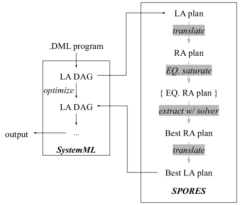
Figure 13: Architecture of SPORES and integration within SystemML

4 Evaluation

We evaluate SPORES to answer three research questions about our approach of relational equality saturation:

• Section 4.1: can SPORES derive hand-coded rewrite rules for sum-product optimization?

• Section 4.2: can SPORES find optimizations that lead to greater performance improvement than hand-coded rewrites and heuristics?

• Section 4.3: does SPORES induce compilation overhead afforded by its performance gain?

We ran experiments on a single node with Intel E74890 v2 @ 2.80GHz with hyper-threading, 1008 GB RAM, 8TB disk, and Ubuntu 16.04.6. We used OpenJDK 1.8.0, Apache Hadoop 2.7.3, and Apache Spark 2.4.4. Spark was configured to run locally with 6 executors, 8 cores/executor, 50GB driver memory, and 100GB executor memory. Our baselines are from Apache SystemML 1.2.0. All datasets have been synthetically generated to evaluate a range of scenarios, where we used algorithm specific data generators from SystemML’s benchmark suite.

4.1 Completeness of Relational Rules

Method Name	#	Example Rewrite
UnnecessaryOuterProduct	3	X*(Y%*%1) -> X*Y, if Y col vector
ColwiseAgg	3	colsums(X) -> sum(X) or X, if col/row vector
RowwiseAgg	3	rowsums(X) -> sum(X) or X, if row/col vector
ColSumsMVMult	1	colSums(X*Y) -> t(Y) %*% X, if Y col vector
RowSumsMVMult	1	rowSums(X*Y) -> X %*% t(Y), if Y row vector
UnnecessaryAggregate	9	sum(X) -> as.scalar(X), if 1x1 dims
EmptyAgg	3	sum(X) -> 0, if nnz(X)==0
EmptyReorgOp	5	t(X) -> matrix(0, ncol(X), nrow(X)) if nnz(X)==0
EmptyMMult	1	X%*%Y -> matrix(0,...), if nnz(Y)==0
IdentityRepMatrixMult	1	X%*%y -> X if y matrix(1,1,1)
ScalarMatrixMult	2	X%*%y -> X*as.scalar(y), if y is a 1-1 matrix
pushdownSumOnAdd	2	sum(A+B) -> sum(A)+sum(B) if dims(A)==dims(B)
DotProductSum	2	sum(v^2) -> t(v)%*%v if ncol(v)==1
reorderMinusMatrixMult	2	(-t(X))%*%y -> -(t(X)%*%y)
SumMatrixMult	3	sum(A%*%B) -> sum(t(colSums(A))*rowSums(B))
EmptyBinaryOperation	3	X*Y -> matrix(0,nrow(X),ncol(X)) / X+Y->X / X-Y->X
ScalarMVBinaryOperation	1	X*y -> X*as.scalar(y), if y is a 1-1 matrix
UnnecessaryBinaryOperation	6	X*1 -> X (after rm unnecessary vectorize)
BinaryToUnaryOperation	3	X*X -> X^2, X+X -> X*2, (X>0)-(X<0) -> sign(X)
MatrixMultScalarAdd	2	eps+U%*%t(V) -> U%*%t(V)+eps
DistributiveBinaryOperation	4	(X-Y*X) -> (1-Y)*X
BushyBinaryOperation	3	(X*(Y*(Z%*%v))) -> (X*Y)*(Z%*%v)
UnaryAggReorgOperation	3	sum(t(X)) -> sum(X)
UnnecessaryAggregates	8	sum(rowSums(X)) -> sum(X)
BinaryMatrixScalarOperation	3	as.scalar(X*s) -> as.scalar(X)*s
pushdownUnaryAggTransposeOp	2	colSums(t(X)) -> t(rowSums(X))
pushdownCSETransposeScalarOp	1	a=t(X), b=t(X^2) -> a=t(X), b=t(X)^2 for CSE t(X)
pushdownSumBinaryMult	2	sum(lamda*X) -> lamda*sum(X) if lamdba is scalar
UnnecessaryReorgOperation	2	t(t(X))->X potentially introduced by other rewrites
TransposeAggBinBinaryChains	2	t(t(A)%*%t(B)+C) -> B%*%A+t(C)
UnnecessaryMinus	1	-(-X)->X potentially introduced by other rewrites

Figure 14: Sum-product rewrites in SystemML. The first column lists the name for each rewrite method. Each method implements a number of rewrite patterns, and the second column shows how many. The last column shows an example rewrite for each method. Following SystemML’s notation, scalars are in lower-case and matrices/vectors in upper-case. %*% is matrix multiply, t() is transpose, and nnz(X) is the number of non-zeroes in $X$. Equality saturation derives rewrites form all 31 methods (84 patterns) with relational rules.

Theoretically, our first hypothesis is validated by the fact that our relational equality rules are complete w.r.t. linear algebra semantics. To test completeness in practice, our first set of experiments check if SPORES can derive the hand-coded sum product rewrite rules in SystemML. To do this, we input the left hand side of each rule into SPORES, perform equality saturation, then check if the rule’s right hand side is present in the saturated graph. The optimizer is able to derive all 84 sum-product rewrite rules in SystemML using relational equality rules. See Figure 14 for a list of these rewrites. We believe replacing the 84 ad-hoc rules with our translation rules $R_{LR}$ and equality rules $R_{EQ}$ would greatly simplify SystemML’s codebase. Together with equality saturation, our relational rules can also lead to better performance, as we demonstrate in the next set of experiments.

4.2 Run Time Measurement

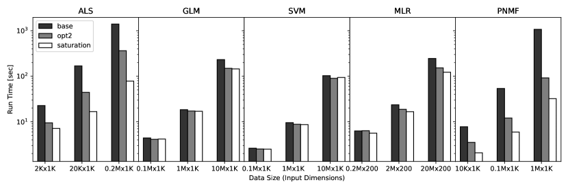
Figure 15: Run time of programs compiled by different optimizers.

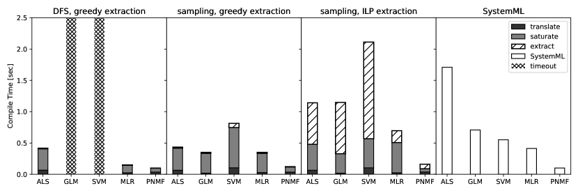
Figure 16: Compile time breakdown for different saturation and extraction strategies. Depth-first saturation reaches the 2.5s timeout compiling GLM and SVM.

We compare SPORES against SystemML’s native optimizations for their performance impact. In particular, we run SystemML with optimization level 2 (opt2), which is its default and includes all advanced rewrites like constant folding and common subexpression elimination. We additionally enable SystemML’s native sum-product rewrites and operator fusion. For baseline (base) we use level 1 optimization from SystemML, since level 0 (no optimization) timeouts on almost all input sizes. base includes no advanced rewrites, sum-product optimization or operator fusion; it only performs local optimizations with basic pattern-matching. We compile and execute 5 real-world algorithms under 3 configurations: 1. SystemML without optimization, 2. SystemML with optimization configured as above, and 3. our equality saturation optimizer. The algorithms include Generalized Linear Model (GLM), Multinomial Logistic Regression (MLR), Support Vector Machine (SVM), Poisson Nonnegative Matrix Factorization (PNMF), and Alternating Least Square Factorization (ALS). We take the implementation of these algorithms from SystemML’s performance benchmark suite.

Figure 15 shows the performance improvement for each optimization setting. Overall, equality saturation is competitive with the hand-coded rules in SystemML: for GLM and SVM, saturation discovers the same optimizations that improve performance as SystemML does. For ALS, MLR and PNMF, saturation found new optimizations that lead to speedups from 1.2X to 5X as compared to SystemML. We analyze each benchmark in detail in the following paragraphs.

For ALS, SPORES leads to up to 5X speedup beyond SystemML’s optimizations using our relational rules. Investigating the optimized code reveals the speedup comes from a rather simple optimization: SPORES expands $(UV^{T}-X)V$ to $UV^{T}V-XV$ to exploit the sparsity in $X$. Before the optimization, all three operations (2 matrix multiply and 1 minus) in the expression create dense intermediates because $U$ and $V$ are dense. After the optimization, $XV$ can be computed efficiently thanks to the sparsity in $X$. $UV^{T}V$ can be computed in one go without intermediates, taking advantage of SystemML’s mmchain operator for matrix multiply chains. Although the optimization is straightforward, it is counter-intuitive because one expects computing $A(B+C)$ is more efficient than $AB+AC$ if one does not consider sparsity. For the same reason, SystemML simply does not consider distributing the multiplication and misses the optimization.

For PNMF, the speedup of up to 3X using RA rules attributes to rewriting $sum(WH)$ to $sum_{col}(W)\cdot sum_{row}(H)$ which avoids materializing a dense intermediate $WH$. Interestingly, SystemML includes this rewrite rule but did not apply it during optimization. In fact, SystemML only applies the rule when $WH$ does not appear elsewhere, in order to preserve common subexpression. However, although $WH$ is shared by another expression in PNMF, the other expression can also be optimized away by another rule. Because both rules uses heuristics to favor sharing CSE, neither fires. This precisely demonstrates the limitation of heuristics.

For MLR, the important optimization by saturation is $P*X-P*sum_{row}(P)*X$ to $P*(1-P)*X$, where $P$ is a column vector. This takes advantage of the sprop fused operator in SystemML to compute $P*(1-P)$, therefore allocating only one intermediate. Note that the optimization factors out $P$, which is the exact opposite to the optimization in ALS that distributes multiply. Naive rewrite rules would have to choose between the two directions, or resort to heuristics to decide when to pick which.

For SVM and GLM, equality saturation finds the same optimizations as SystemML does, leading to speedup mainly due to operator fusion. Upon inspection, we could not identify better optimizations for SVM. For GLM, however, we discovered a manual optimization that should improve performance in theory, but did not have an effect in practice since SystemML cannot accurately estimate sparsity to inform execution.

4.3 Compilation Overhead

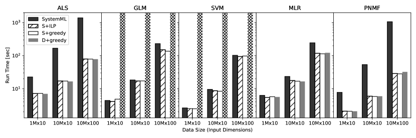
Figure 17: Performance impact of different saturation and extraction strategies. S is saturation with sampling, and D is depth-first saturation. Depth-first saturation runs into timeout compiling GLM and SVM.

In our initial experiments, SPORES induces nontrivial compilation overhead compared to SystemML’s native rule-based rewrites. Figure 16 (sampling, ILP extraction) shows the compile time breakdown for each benchmark, and the majority of time is spent in the ILP solver. We therefore experiment with a greedy algorithm during extraction to see if we can trade off guarantees of optimality for a shorter compile time. This algorithm traverses the saturated graph bottom-up, picking the cheapest operator in each class at every level. Figure 17 shows the performance impact of greedy extraction, and Figure 16 (sampling, greedy extraction) shows the compile time with it. Greedy extraction significantly reduces compile time without sacrificing any performance gain! This is not surprising in light of the optimizations we discussed in Section 4.2: all of these optimizations improve performance regardless of common subexpressions, so they are selected by both the ILP-based and the greedy extractor.

We also compare saturation with sampling against depth-first saturation in terms of performance impact and compile time. Recall the depth-first saturation strategy applies all matches per rule per iteration. As Figure 16 shows, sampling is slightly slower for ALS, MLR and PNMF, but resolves the timeout for GLM and SVM. This is because sampling takes longer to converge when full saturation is possible, and otherwise prevents the graph from blowing up before reaching the iteration limit. Indeed, saturation converges for ALS, MLR and PNMF, which means SPORES can guarantee the optimality of its result under the given cost model. Saturation does not not converge before reaching the iteration limit for GLM and SVM because of deeply nested $*$ and $+$ in the programs. Convergence may come as a surprise despite E-Graph’s compaction – expansive rules like associativity and commutativity commonly apply in practice. However, the expression DAGs we encounter are often small (no more than 15 operators), and large DAGs are cut into small pieces by optimization barriers like uninterpreted functions.

Figure 16 compares the overall DAG compilation overhead of SystemML against SPORES with different extraction strategies. Note that the overhead of SystemML also includes optimizations unrelated to sum-product rewrites that are difficult to disentangle, therefore it only gives a sense of the base compilation time and does not serve as head-to-head comparison against SPORES. Although SPORES induces significant compilation overhead in light of SystemML’s total DAG compilation time, the overhead is afforded by its performance gain. As we did not focus our efforts on reducing compile time, we believe there is plenty room for improvement, for example organizing rewrite rules to speed up saturation.

5 Related Work

There is a vast body of literature for both relational query optimization and optimizing compilers for machine learning. Since we optimize machine learning programs through a relational lens, our work relates to research in both fields. As we have pointed out, numerous state-of-the-art optimizing compilers for machine learning resort to syntactic rewrites and heuristics to optimize linear algebra expressions [1] [27] [11]. We distinguish our work which performs optimization based on a relational semantics of linear algebra and holistically explore the complex search space. A majority of relational query optimization focus on join order optimization [7] [19] [20] [25]; we distinguish our work which optimizes programs with join (product), union (addition), and aggregate (sum) operations. Sum-product optimization considers operators other than join while optimizing relational queries. Recent years have seen a line of excellent theoretical and practical research in this area [17] [14]. These work gives significant improvement for queries involving $*$ and $\sum$, but fall short of LA workloads that occur in practice. We step past these frameworks by incorporating common subexpressions and incorporating addition ($+$).

In terms of approach, our design of relational IR ties in to research that explores the connection between linear algebra and relational algebra. Our design and implementation of the optimizer ties into research that leverage equality saturation and and-or dags for query optimization and compiler optimization for programming languages. Since we focus on optimizing sum-product expressions in linear algebra, our work naturally relates to research in sum-product optimization. We now discuss these three lines of research in detail.

5.1 Relational Algebra and Linear Algebra

Elgamal et al. [5] envisions spoof, a compiler for machine learning programs that leverages relational query optimization techniques for LA sum-product optimization. We realize this vision by providing the translation rules from LA to RA and the relational equality rules that completely represents the search space for sum-product expressions. One important distinction is, Elgamal et al. proposes restricted relational algebra where every expression must have at most two free attributes. This ensures every relational expression in every step of the optimization process to be expressible in LA. In contrast, we remove this restriction and only require the optimized output to be in linear algebra. This allows us to trek out to spaces not covered by linear algebra equality rules and achieve completeness. In addition to sum-product expressions, Elgamal et al. also considers selection and projection operations like selecting the positive entries of a matrix. We plan to explore supporting selection and projection in the future. Elgamal et al. also proposes compile-time generation of fused operators, which is implemented by Boehm et al. [2]. SPORES readily takes advantage of existing fused operators, and we plan to explore combining sum-product rewrite with fusion generation in the future.

MorpheusFI by Li et al. [18] and LARA by Hutchison et al. [12] explore optimizations across the interface of machine learning and database systems. In particular, MorpheusFI speeds up machine learning algorithms over large joins by pushing computation into each joined table, thereby avoiding expensive materialization. LARA implements linear algebra operations with relational operations and shows competitive optimizations alongside popular data processing systems. Schleich et al.[24] and Khamis et al.[16] explore in-database learning, which aims to push entire machine learning algorithms into the database system. We contribute in this space by showing that even without a relational engine, the relational abstraction can still benefit machine learning tasks as a powerful intermediate abstraction.

5.2 Equality Saturation and AND-OR DAGs

Equality saturation and and-or dags have been applied to optimize low-level assembly code [15], Java programs [28], database queries [7], floating point arithmetics [23], and even computer-aided design models [21]. The design of our relational IR brings unique challenges in adopting equality saturation. Compared to database query optimizers that focus on optimizing join orders, unions and aggregates play a central role in our relational IR and are prevalent in real-world programs. As a result, our equality rules depend on the expression schema which is not immediately accessible from the syntax. We propose class invariants as a solution to access schema information, and show it to be a powerful construct that enables constant folding and improves cost estimation. Compared to optimizers for low-level assembly code or Java program, we commonly encounter linear algebra expressions that trigger expansive rules and make saturation convergence impractical. We propose to sample rewrite matches in order to achieve good exploration without full saturation. Equality saturation takes advantage of constraint solvers which have also been applied to program optimization and query optimization. In particular, the use of solvers for satisfiability modulo theories by [26] has spawned a paradigm now known as program synthesis. In query optimization research, [29] applies Mixed Integer Linear Programming for optimizing join ordering. Although constraint solvers offer pleasing guarantees of optimality, our experiments show their overhead does not bring significant gains for optimizing LA expressions.

6 Conclusion

We propose a novel optimization approach for compiling linear algebra programs, using relational algebra as an intermediate representation and equality saturation to explore the search space. We implement our equality saturation based optimizer and show it is effective for improving real-world machine learning algorithms.

7 Acknowledgement

The authors would like to thank Alexandre Evfimievski, Matthias Boehm, and Berthold Reinwald for their insights in developing SystemMLs internals. We would also like to thank Mathew Luo and Brendan Murphy for their guidance in piloting an ILP extractor as well as Zach Tatlock, Max Willsey and Chandrakana Nandi for their valuable feedback and discussion.

Appendix A Uniqueness of RA Canonical Form

To prove Lemma 2.2 (uniqueness of canonical form), we first give formal definitions for several important constructs. First, we interpret a tensor (high dimensional matrix) as a function from a tuple of indices to a real number:

Definition A.1.

(Tensors) A tensor is a function $A:[N]^{d}\rightarrow\mathbb{R}$ such that $A(i,j,\dots)$ returns the tensor entry $A_{ij\dots}$. $d$ is the dimensionality of $A$, and $N$ is the dimension size. Each argument to $A$ is an index, and we write $i$ (in bold) for a tuple of indices. We write $\boldsymbol{A}$ (in bold) for $A(\boldsymbol{i})$, i.e. a tensor indexed with a tuple of indices.

We use the terms tensor and relation interchangingly. Note that we assume every dimension has the same size $N$ for simplicity. If the dimension sizes differ in a tensor $A$, we can easily set $N$ to be the maximum size and fill $A$ with zeroes accordingly. For example, for a 2D matrix $A$ with dimensions $|d_{1}|=m<|d_{2}|=n$, we simply set $N=n$ and have $A_{ij}=0$ for $i>m$.

Now we give names for special forms of expressions at each level of the normal form:

Definition A.2.

(Atoms, Monomials, Terms, Polyterms) An indexed tensor $\boldsymbol{A}$ is also called an atom. A monomial $m$ is a product of any number of atoms. A term $t$ is an aggregate of a monomial over a set of indices. A polyterm $e$ is the sum of terms (with a constant term $c$ at the end), where each term has a constant factor:

$$\boldsymbol{A} :=A(\boldsymbol{i}) (1)\,atoms$$

$$m :=\boldsymbol{A}_{1}\times\boldsymbol{A}_{2}\times\dots\boldsymbol{A}_{n} (2)\,monomials$$

$$t :=\textstyle\sum_{\boldsymbol{i}}m (3)\,terms$$

$$e :=c_{1}t_{1}+c_{2}t_{2}+\dots c_{n}t_{n}+c\, (4)\,polyterms$$

We identify the monomial $m$ with a bag of atoms, denoted $bag(m)$, such that for every atom $\boldsymbol{A}$ occurring $n$ times in $m$, $bag(m)$ contains $n$ copies of $\boldsymbol{A}$. An index $i$ in a term $t=\sum_{\boldsymbol{i}}m$ is bound if $i\in\boldsymbol{i}$; otherwise it is free. We write $bv(t)$ for the set of bound indices in $t$, $fv(t)$ for the set of free indices in $t$, and $vars(t)$ for the set of all indices in $t$.

Example 1.

The polyterm $2\sum_{j}A(i,j)\times A(i,j)\times B(j,k)\times B(j,k)+3\sum_{l}A(i,l)\times C(l,k)+2$ represents the linear algebra expression $2A^{2}B^{2}+3AC+2$, where $A^{2}$ squares the matrix element-wise. The monomial $A(i,j)\times A(i,j)\times B(j,k)\times B(j,k)$ is the same as $A(i,j)\times B(j,k)\times A(i,j)\times B(j,k)$, and we view it as the bag $\{A(i,j),A(i,j),B(j,k),B(j,k)\}$.

Before giving the formal definition of a canonical form, we need to define two syntactical relationships between our expressions, namely homomorphism and isomorphism. Fix terms $t=\sum_{\boldsymbol{i}}m$ and $t^{\prime}=\sum_{\boldsymbol{i^{\prime}}}m^{\prime}$, and let $f:\boldsymbol{i}\rightarrow\boldsymbol{i}^{\prime}$ be any function. Let $\boldsymbol{A}\in bag(m)$ be an atom of $m$. We write $f(A)$ for the result of applying $f$ to all bound indices of $\boldsymbol{A}$. We write $f(bag(m))$ for the bag obtained by applying $f$ to each atom $\boldsymbol{A}\in bag(m)$.

Definition A.3.

(Term Homomorphism) A homomorphism $f:t\rightarrow t^{\prime}$ is a function $f:\boldsymbol{i}\rightarrow\boldsymbol{i}^{\prime}$ such that $f(bag(m))=bag(m^{\prime})$. Note that $f$ is a one-to-one mapping between $bag(m)$ and $bag(m^{\prime})$.

Example 2.

Between terms $t_{1}=\sum_{vwst}A(i,v)\times B(v,w)\times A(i,s)\times B(s,t)$ and $t_{2}=\sum_{jk}A^{2}(i,j)\times B^{2}(j,k)$ there is a homomorphism:

$$t_{1}\rightarrow t_{2}:[v\mapsto j,w\mapsto k,s\mapsto j,t\mapsto k]$$

We extend $f$ to take $vars(t_{1})$ where free variables map to themselves. It is easy to see for any homomorphism $f$, $f(vars(t_{1}))=vars(t_{2})$.

Corollary 1.

Homomorphism is surjective on the indices.

Proof.

Suppose for the sake of contradiction that a homomorphism $f:t_{1}\rightarrow t_{2}$ is not surjective. Then there exists an index $i\in vars(t_{2})$ that is not in $f(vars(t_{1}))$, and the atom containing $i$ does not appear in $f(t_{1})$. That implies the monomial in $f(t_{1})$ is cannot be equal to the monomial in $t_{2}$, so $f$ is not a homomorphism – contradiction. ∎

Corollary 2.

Homomorphism is closed under composition: given homomorphisms $f:t_{1}\rightarrow t_{2}$ and $g:t_{2}\rightarrow t_{3}$, $g\circ f:t_{1}\rightarrow t_{3}$ is a homomorphism from $t_{1}$ to $t_{3}$.

Proof.

A homomorphism is a function on indices, so composing homomorphisms is just composing functions. ∎

A stronger correspondence between terms is an isomorphism:

Definition A.4 (Term Isomorphism).

Terms $t_{1}=\sum_{\boldsymbol{i_{1}}}m_{1}$ and $t_{2}=\sum_{\boldsymbol{i_{2}}}m_{2}$ are isomorphic iff there is a bijective homomorphism between them. We write $t_{1}\equiv t_{2}$ to mean $t_{1}$ and $t_{2}$ are isomorphic.

A pair of homomorphisms $t_{1}\rightarrow t_{2}$ and $t_{2}\rightarrow t_{1}$ produce an isomorphism:

Lemma A.1.

Given two terms $t_{1}$ and $t_{2}$, if there is a homomorphism $f:t_{1}\rightarrow t_{2}$ and a homomorphism $g:t_{2}\rightarrow t_{1}$ then $t_{1}\equiv t_{2}$. If there is a cycle of homomorphisms among a number of terms, all terms on the cycle are isomorphic.

Proof.

By Corollary 1, a pair of homomorphisms between two terms are a pair of surjective maps between the terms’ indices. A pair of surjective maps induce a bijective map which is an isomorphism. By Corollary 2, if $t_{1}$ and $t_{2}$ are on a cycle of homomorphism, we can retract the homomorphism chains between them to obtain a pair of homomorphisms $f:t_{1}\rightarrow t_{2}$ and $g:t_{2}\rightarrow t_{1}$, which implies $t_{1}\equiv t_{2}$. ∎

We are now ready to formally define the canonical form for RA expressions:

Definition A.5.

(Canonical Form) An RPlan expression (as defined in Table 1) is canonical if it is a polyterm (Definition A.2) containing no isomorphic terms.

Our ultimate goal is to identify canonical form isomorphism with equivalence. That is, two canonical expressions are equivalent iff they are isomorphic. By equivalence we mean the expressions evaluate to the same result given any same inputs:

Definition A.6.

(Equivalence of Expressions) Two expressions are equivalent iff $\forall\boldsymbol{T}.e_{1}(\boldsymbol{T})=e_{2}(\boldsymbol{T})$, where $\boldsymbol{T}$ is the set of input tensors to the expressions. We write $e_{1}=e_{2}$ to mean $e_{1}$ and $e_{2}$ are equivalent.

We can canonicalize any expression by pulling $+$ to the top and pushing $\times$ to the bottom, while combining isomorphic terms $c_{1}t+c_{2}t$ into $(c_{1}+c_{2})t$:

Lemma A.2.

For every RPlan expression, there is an equivalent canonical expression.

Proof.

The proof is a standard application of the rewrite rules $R_{EQ}$ in Figure 3. ∎

We can identify canonical expressions syntactically using term isomorphism:

Definition A.7.

(Isomorphic Canonical Expressions) Given two canonical expressions $e=\sum_{\boldsymbol{i}}c_{1}t_{1}+\dots+c_{n}t_{n}+c$ and $e^{\prime}=\sum_{\boldsymbol{i^{\prime}}}c_{1}^{\prime}t_{1}^{\prime}+\dots+c_{m}^{\prime}t_{m}^{\prime}+c^{\prime}$, $e$ and $e^{\prime}$ are isomorphic if there is a bijection $\sigma:[n]\rightarrow[m]$ (in particular $n=m$), such that $\forall i\in[n]$, $c_{i}=c_{\sigma(i)}^{\prime}$, $t_{i}\equiv t_{\sigma(i)}^{\prime}$, and $c=c^{\prime}$.

Note that isomorphic expressions have the same free variables. We now show two expressions are isomorphic iff they are equivalent:

Theorem A.3.

(Isomorphism Captures Equivalence) For canonical expressions $e_{1}$ and $e_{2}$:

$$e_{1}\equiv e_{2}\iff e_{1}=e_{2}$$

Proof.

The left-to-right direction is straightforward: isomorphism only renames indices and reorders $+$ and $\times$, which does not change semantics. And because RA semantics is deterministic, two isomorphic expressions compute the same function.

The right-to-left direction is exactly Lemma 2.2, the uniqueness of canonical forms:

$$e_{1}=e_{2}\Rightarrow e_{1}\equiv e_{2}$$

Without loss of generality, we make the following simplifying assumptions. First, we assume $e_{1}$ and $e_{2}$ contain no constant terms. Otherwise the expressions would evaluate to their respective constants on all-0 inputs, so the constant terms must be equal. Subtracting the same constant preserves equivalence and isomorphism, so we can simply remove equal constant terms. Second, we assume no term in $e_{1}$ is isomorphic to any term in $e_{2}$. Otherwise if $e_{1}$ contains $c_{1}t_{1}$ and $e_{2}$ contains $c_{2}t_{2}$ with $t_{1}\equiv t_{2}$, then we can write $e_{1}=c_{1}t_{1}+e_{1}^{\prime}$ and $e_{2}=c_{2}t_{2}+e_{2}^{\prime}$ where $e_{1}^{\prime}$ and $e_{2}^{\prime}$ are polyterms. Assume w.l.o.g that $c_{1}\leq c_{2}$. Since $c_{1}t_{1}+e_{1}^{\prime}=c_{2}t_{2}+e_{2}^{\prime}$, $e_{1}^{\prime}=(c_{2}-c_{1})t_{2}+e_{2}^{\prime}$ and we have removed $t_{1}$ from $e_{1}$. Furthermore, $e_{1}=e_{2}\Rightarrow e_{1}^{\prime}=e_{2}^{\prime}$ and $e_{1}^{\prime}\equiv e_{2}^{\prime}\Rightarrow e_{1}\equiv e_{2}$. Then by proving $e_{1}^{\prime}=e_{2}^{\prime}\Rightarrow e_{1}^{\prime}\equiv e_{2}^{\prime}$ we can show the following:

$$e_{1}=e_{2}\Rightarrow e_{1}^{\prime}=e_{2}^{\prime}\Rightarrow e_{1}^{\prime}\equiv e_{2}^{\prime}\Rightarrow e_{1}\equiv e_{2}$$

Finally we assume $e_{1}$ and $e_{2}$ are fully aggregated, i.e. every index is bound. Without this assumption, we first observe $e_{1}$ and $e_{2}$ must have the same free indices to output tensors with the same dimensionality. Then we define $e_{1}^{\prime}=\sum_{\boldsymbol{i}}e_{2}$ and $e_{2}^{\prime}=\sum_{\boldsymbol{i}}e_{2}$, where $\boldsymbol{i}$ is the set of free variables of $e_{1}$ and $e_{2}$. We can easily show $e_{1}=e_{2}\Rightarrow e_{1}^{\prime}=e_{2}^{\prime}$ and $e_{1}^{\prime}\equiv e_{2}^{\prime}\Rightarrow e_{1}\equiv e_{2}$, and with a proof of $e_{1}^{\prime}=e_{2}^{\prime}\Rightarrow e_{1}^{\prime}\equiv e_{2}^{\prime}$ it follows $e_{1}=e_{2}\Rightarrow e_{1}\equiv e_{2}$.

Each expression can now be viewed as a set of terms, where each term has a constant factor and no two terms are isomorphic. Denoting by $t_{1}<t_{2}$ if there is a homomorphism $t_{1}\rightarrow t_{2}$, we observe homomorphism induces a partial order on the terms of $e_{1}$ and $e_{2}$. There is no cycle of homomorphisms, because by Lemma A.1 such a cycle implies isomorphisms, but we have assumed no isomorphic terms.

We now prove Lemma 2.2 through its contrapositive:

$$e_{1}\not\equiv e_{2}\Rightarrow e_{1}\not=e_{2}$$

We proceed by constructing a set of witness input tensors given which $e_{1}$ and $e_{2}$ return different results. First, let $t_{1}=\sum_{i_{1}i_{2}\dots}\boldsymbol{X}_{1}\times\boldsymbol{X}_{2}\times\dots$ be the minimal term under the partial order induced by homomorphism. Assume w.l.o.g $t_{1}\in e_{1}$. Define bijective function $\phi:i_{n}\rightarrow n$ mapping each index to a unique number. For each $\boldsymbol{X}_{n}=X_{n}(\boldsymbol{i}_{n})$ introduce a real-valued variable $x_{n}$ and construct the input tensor $X_{n}$ such that $X_{\boldsymbol{i}_{n}}=x_{n}$. Finally, set all undefined entries of each input tensor to $0$.

Given the input tensors defined above, $t_{1}$ evaluates to a polynomial $p_{1}$ of variables $x_{1}\dots x_{n}$. Every monomial in $p_{1}$ corresponds to a function from $t_{1}$’s atoms $\boldsymbol{X}_{a},\boldsymbol{X}_{b},\dots$ to some variables $x_{m},x_{n},\dots$, and we call such a function $f_{m}$. There is one special (bijective) $f_{m}$ that maps each atom to its own variable: let $m_{1}$ be the monomial in $t_{1}$, $m_{1}=\boldsymbol{X}_{1}\times\boldsymbol{X}_{2}\times\dots$. We define $f_{p}(t_{1})=m_{1}(\phi(i_{1}),\phi(i_{2}),\dots)=x_{1}x_{2}\dots$. $f_{p}(t_{1})$ does not appear in any polynomial from other terms. Otherwise if it appears in polynomial $p_{2}$ from term $t_{2}$, we would be able to construct a homomorphism $t_{2}\rightarrow t_{1}=f_{m}\circ f_{p}^{-1}$, where $f_{m}$ maps the monomial $m_{2}$ in $p_{2}$ to $t_{1}$. But that is impossible because we have picked $t_{1}$ to be the minimal term under homomorphism. Therefore, $p_{1}$ differs from any polynomial from terms in $t_{2}$, and by the fundamental theorem of algebra the polynomial are inequivalent. As a result, $e_{1}\not=e_{2}$. ∎

References

- [1] M. Boehm. Apache systemml. In S. Sakr and A. Y. Zomaya, editors, Encyclopedia of Big Data Technologies. Springer, 2019.
- [2] M. Boehm, B. Reinwald, D. Hutchison, P. Sen, A. V. Evfimievski, and N. Pansare. On optimizing operator fusion plans for large-scale machine learning in systemml. PVLDB, 11(12):1755–1768, 2018.
- [3] S. Chaudhuri and M. Y. Vardi. Optimization of Real conjunctive queries. In Proceedings of the Twelfth ACM SIGACT-SIGMOD-SIGART Symposium on Principles of Database Systems, May 25-28, 1993, Washington, DC, USA, pages 59–70, 1993.
- [4] S. Cohen, Y. Sagiv, and W. Nutt. Equivalences among aggregate queries with negation. ACM Trans. Comput. Log., 6(2):328–360, 2005.
- [5] T. Elgamal, S. Luo, M. Boehm, A. V. Evfimievski, S. Tatikonda, B. Reinwald, and P. Sen. SPOOF: Sum-Product Optimization and Operator Fusion for Large-Scale Machine Learning. In CIDR, 2017.
- [6] C. Forgy. Rete: A fast algorithm for the many patterns/many objects match problem. Artif. Intell., 19(1):17–37, 1982.
- [7] G. Graefe. The Cascades Framework for Query Optimization. IEEE Data Eng. Bull., 18(3), 1995.
- [8] T. J. Green. Containment of conjunctive queries on annotated relations. In Database Theory - ICDT 2009, 12th International Conference, St. Petersburg, Russia, March 23-25, 2009, Proceedings, pages 296–309, 2009.
- [9] T. J. Green, G. Karvounarakis, and V. Tannen. Provenance semirings. In L. Libkin, editor, Proceedings of the Twenty-Sixth ACM SIGACT-SIGMOD-SIGART Symposium on Principles of Database Systems, June 11-13, 2007, Beijing, China, pages 31–40. ACM, 2007.
- [10] L. Gurobi Optimization. Gurobi optimizer reference manual, 2019.
- [11] B. Huang, S. Babu, and J. Yang. Cumulon: optimizing statistical data analysis in the cloud. In K. A. Ross, D. Srivastava, and D. Papadias, editors, Proceedings of the ACM SIGMOD International Conference on Management of Data, SIGMOD 2013, New York, NY, USA, June 22-27, 2013, pages 1–12. ACM, 2013.
- [12] D. Hutchison, B. Howe, and D. Suciu. Laradb: A minimalist kernel for linear and relational algebra computation. CoRR, abs/1703.07342, 2017.
- [13] Y. E. Ioannidis and R. Ramakrishnan. Containment of conjunctive queries: Beyond relations as sets. ACM Trans. Database Syst., 20(3):288–324, 1995.
- [14] M. R. Joglekar, R. Puttagunta, and C. Ré. Ajar: Aggregations and joins over annotated relations. In PODS. ACM, 2016.
- [15] R. Joshi, G. Nelson, and K. H. Randall. Denali: A goal-directed superoptimizer. In J. Knoop and L. J. Hendren, editors, Proceedings of the 2002 ACM SIGPLAN Conference on Programming Language Design and Implementation (PLDI), Berlin, Germany, June 17-19, 2002, pages 304–314. ACM, 2002.
- [16] M. A. Khamis, H. Q. Ngo, X. Nguyen, D. Olteanu, and M. Schleich. In-database learning with sparse tensors. CoRR, abs/1703.04780, 2017.
- [17] M. A. Khamis, H. Q. Ngo, and A. Rudra. FAQ: Questions Asked Frequently. In PODS. ACM, 2016.
- [18] S. Li, L. Chen, and A. Kumar. Enabling and optimizing non-linear feature interactions in factorized linear algebra. In P. A. Boncz, S. Manegold, A. Ailamaki, A. Deshpande, and T. Kraska, editors, Proceedings of the 2019 International Conference on Management of Data, SIGMOD Conference 2019, Amsterdam, The Netherlands, June 30 - July 5, 2019, pages 1571–1588. ACM, 2019.
- [19] G. Moerkotte and T. Neumann. Analysis of Two Existing and One New Dynamic Programming Algorithm for the Generation of Optimal Bushy Join Trees without Cross Products. In VLDB, 2006.
- [20] G. Moerkotte and T. Neumann. Dynamic Programming Strikes Back. In SIGMOD, 2008.
- [21] C. Nandi, A. Anderson, M. Willsey, J. R. Wilcox, E. Darulova, D. Grossman, and Z. Tatlock. Using e-graphs for CAD parameter inference. CoRR, abs/1909.12252, 2019.
- [22] C. G. Nelson. Techniques for Program Verification. PhD thesis, Stanford University, Stanford, CA, USA, 1980. AAI8011683.
- [23] P. Panchekha, A. Sanchez-Stern, J. R. Wilcox, and Z. Tatlock. Automatically improving accuracy for floating point expressions. In D. Grove and S. Blackburn, editors, Proceedings of the 36th ACM SIGPLAN Conference on Programming Language Design and Implementation, Portland, OR, USA, June 15-17, 2015, pages 1–11. ACM, 2015.
- [24] M. Schleich, D. Olteanu, and R. Ciucanu. Learning linear regression models over factorized joins. In F. Özcan, G. Koutrika, and S. Madden, editors, Proceedings of the 2016 International Conference on Management of Data, SIGMOD Conference 2016, San Francisco, CA, USA, June 26 - July 01, 2016, pages 3–18. ACM, 2016.
- [25] P. G. Selinger, M. M. Astrahan, D. D. Chamberlin, R. A. Lorie, and T. G. Price. Access path selection in a relational database management system. In Proceedings of the 1979 ACM SIGMOD international conference on Management of data, pages 23–34. ACM, 1979.
- [26] A. Solar-Lezama, L. Tancau, R. Bodík, S. A. Seshia, and V. A. Saraswat. Combinatorial sketching for finite programs. In J. P. Shen and M. Martonosi, editors, Proceedings of the 12th International Conference on Architectural Support for Programming Languages and Operating Systems, ASPLOS 2006, San Jose, CA, USA, October 21-25, 2006, pages 404–415. ACM, 2006.
- [27] A. K. Sujeeth, H. Lee, K. J. Brown, T. Rompf, H. Chafi, M. Wu, A. R. Atreya, M. Odersky, and K. Olukotun. Optiml: An implicitly parallel domain-specific language for machine learning. In L. Getoor and T. Scheffer, editors, Proceedings of the 28th International Conference on Machine Learning, ICML 2011, Bellevue, Washington, USA, June 28 - July 2, 2011, pages 609–616. Omnipress, 2011.
- [28] R. Tate, M. Stepp, Z. Tatlock, and S. Lerner. Equality saturation: A new approach to optimization. Logical Methods in Computer Science, 7(1), 2011.
- [29] I. Trummer and C. Koch. Solving the join ordering problem via mixed integer linear programming. In S. Salihoglu, W. Zhou, R. Chirkova, J. Yang, and D. Suciu, editors, Proceedings of the 2017 ACM International Conference on Management of Data, SIGMOD Conference 2017, Chicago, IL, USA, May 14-19, 2017, pages 1025–1040. ACM, 2017.
- [30] M. Willsey, C. Nandi, Y. R. Wang, O. Flatt, Z. Tatlock, and P. Panchekha. egg: Fast and extensible equality saturation, 2020.