Charge-Density Wave Order on a $\pi$-flux Square Lattice

Abstract

The effect of electron-phonon coupling (EPC) on Dirac fermions has recently been explored numerically on a honeycomb lattice, leading to precise quantitative values for the finite temperature and quantum critical points. In this paper, we use the unbiased determinant Quantum Monte Carlo (DQMC) method to study the Holstein model on a half-filled staggered-flux square lattice, and compare with the honeycomb lattice geometry, presenting results for a range of phonon frequencies $0.1\leqslant\omega\leqslant 2.0$. We find that the interactions give rise to charge-density wave (CDW) order, but only above a finite coupling strength $\lambda_{\rm crit}$. The transition temperature is evaluated and presented in a $T_{c}$-$\lambda$ phase diagram. An accompanying mean-field theory (MFT) calculation also predicts the existence of quantum phase transition (QPT), but at a substantially smaller coupling strength.

I I. Introduction

The physics of massless Dirac points, as exhibited in the band structure of the honeycomb lattice of graphene, has driven intense studyCastro Neto et al. (2009); Geim (2009); Choi et al. (2010); Novoselov et al. (2012). The square lattice with $\pi$-flux per plaquette is an alternate tight-binding Hamiltonian which also contains Dirac points in its band structure. Initial investigations of the $\pi$-flux model focused on the non-interacting limit(Harris et al., 1989), but, as with the honeycomb lattice, considerable subsequent effort has gone into extending this understanding to incorporate the effect of electron-electron interactions. Numerical simulations of the Hubbard Hamiltonian with an on-site repulsion $U$ between spin up and spin down fermions, including Exact Diagonalization (Jia et al., 2013) and Quantum Monte Carlo (QMC)Otsuka and Hatsugai (2002); Otsuka et al. (2014); Li et al. (2015); Toldin et al. (2015); Otsuka et al. (2016); Lang and Läuchli (2019); Guo et al. (2018a, b) revealed a quantum phase transition at $U_{c}\sim 5.55\,t$ into a Mott antiferromagnetic (AF) phase in the chiral Heisenberg Gross-Neveu universality class. For a spinless fermion system with near-neighbor interactions a chiral Ising Gross-Neveu universality class is suggestedWang et al. (2014). These results have been contrasted with those on a honeycomb lattice, which has a similar Dirac point structure, though at a smaller critical interaction $U_{c}\sim 3.85\,t$ Otsuka et al. (2016).

In the case of the repulsive Hubbard Hamiltonian, there were two motivations for studying both the honeycomb and the $\pi$-flux geometries. The first was to verify that the quantum critical transitions to AF order as the on-site repulsion $U$ increases share the same universality class, that of the Gross-Neveu model. The second was to confirm that an intermediate spin-liquid (SL) phase between the semi-metal and AF phasesMeng et al. (2010), which had been shown not to be present on a honeycomb latticeOtsuka et al. (2013), was also absent on the $\pi$-flux geometry.

Studies of the SU(2) $\pi$-flux Hubbard model have also been extended to SU(4), using projector QMCZhou et al. (2018), and to staggered flux where $\pm\pi$ hopping phases alternate on the latticeChang and Scalettar (2012). In the former case, the semi-metal to AF order transition was shown to be replaced by a semi-metal to valence bond solid transition characterized by breaking of a ${\cal Z}_{4}$ symmetry. In the latter work, an intermediate phase with power-law decaying spin-spin correlations was suggested to exist between the semi-metal and AF.

A largely open question is how this physics is affected in the presence of electron-phonon rather than electron-electron interactions. A fundamental Hamiltonian, proposed by Holstein(Holstein, 1959), includes an on-site coupling of electron density to the linear displacement of the phonon field. In the low density limit, extensive numerical work has quantified polaron and bipolaron formation, in which electrons are “dressed’ by an accompanying lattice distortion Kornilovitch (1998, 1999); Alexandrov (2000); Hohenadler et al. (2004); Ku et al. (2002); Spencer et al. (2005); Macridin et al. (2004); Romero et al. (1999). At sufficiently large coupling, electrons or pairs of electrons can become ‘self-trapped’ (localized). One of the most essential features of the Holstein model is that the lattice distortion of one electron creates an energetically favorable landscape for other electrons, so that there is an effective attraction mediated by the phonons. At higher densities, collective phenomena such as Charge-Density Wave (CDW) phases, and superconductivity (SC) have been widely studied (Scalettar et al., 1989; Marsiglio, 1990; Vekic et al., 1992; Niyaz et al., 1993; Vekić and White, 1993; Freericks et al., 1993; Zheng and Zhu, 1997; Jeckelmann et al., 1999; Hohenadler et al., 2004). CDW is especially favored on bipartite lattices and at fillings which correspond to double occupation of one of the two sublattices. SC tends to occur when one dopes away from these commensurate fillings.

Recent work on the Holstein model on the honeycomb lattice suggested a quantum phase transition from semi-metal to gapped CDW order (Zhang et al., 2019; Chen et al., 2019) similar to the results for the Hubbard Hamiltonian. However, a key difference between the Hubbard and Holstein models is the absence of the SU(2) symmetry of the order parameter in the latter case. Thus, while long-range AF order arising from electron-electron interaction occurs only at zero temperature in 2D, the CDW phase transition induced by electron-phonon coupling can occur at finite temperature- the symmetry being broken is that associated with two discrete sub-lattices. For classical phonons ($\omega_{0}=0$), the electron-phonon coupling becomes an on-site energy in the mean-field approximation. In the anti-adiabatic limit where phonon frequencies are set to infinity, the Holstein model maps onto the attractive Hubbard model.

Here we extend the existing work on the effect of EPC on Dirac fermions from the honeycomb geometry to the $\pi$-flux lattice. The $\pi$-flux state is realized by threading half of a magnetic flux quantum through each plaquette of a square latticeAffleck and Marston (1988). Recently it has been experimentally realized in optical lattices using Raman assisted hoppingAidelsburger et al. (2011). There are also theoretical suggestions that the $\pi$-flux lattice might be engineered by the proximity of an Abrikosov lattice of vortices of a type-II superconductor, or via spontaneously generating a $\pi$-flux by coupling fermions to a ${\cal Z}_{2}$ gauge theory in (2+1) dimensionsGazit et al. (2017). The $\pi$-flux hopping configuration has an additional interesting feature motivating our current work: it is the unique magnetic field value which minimizes the ground state energy for non-interacting fermions at half-filled on a bipartite lattice. Indeed, Lieb has shown that this theorem is also true at finite temperature, and furthermore holds in the presence of Hubbard inteactionsLieb (1994). Here we consider the thermodynamics of the $\pi$-flux lattice with EPC.

This paper is organized as follows: in the next section, we describe the Holstein model and the $\pi$-flux square lattice. Section III presents, briefly, a mean-field theory (MFT) for the model. Section IV reviews our primary method, DQMC. Section V contains results from the DQMC simulations, detailing the nature of the CDW phase transition, both the finite temperature transition at fixed EPC, and the QPT which occurs at $T=0$ with varying EPC. Section VI contains our conclusions.

II II. Model

The Holstein model Holstein (1959) describes conduction electrons locally coupled to phonon degrees of freedom,

$$\mathcal{\hat{H}}= -\sum_{\langle\mathbf{i},\mathbf{j}\rangle,\sigma}\big{(}t_{\mathbf{i},\mathbf{j}}\,\hat{d}^{\dagger}_{\mathbf{i}\sigma}\hat{d}^{\phantom{\dagger}}_{\mathbf{j}\sigma}+{\rm h.c.}\big{)}-\mu\sum_{\mathbf{i},\sigma}\hat{n}_{\mathbf{i},\sigma}$$

$$+\frac{1}{2M}\sum_{\mathbf{i}}\hat{P}^{2}_{\mathbf{i}}+\frac{\omega_{\,0}^{2}}{2}\sum_{\mathbf{i}}\hat{X}^{2}_{\mathbf{i}}+\lambda\sum_{\mathbf{i},\sigma}\hat{n}_{\mathbf{i},\sigma}\hat{X}_{\mathbf{i}}\,\,.$$ (1)

The sums on $\mathbf{i}$ and $\sigma$ run over all lattice sites and spins $\sigma=\uparrow,\downarrow$. $\langle\mathbf{i},\mathbf{j}\rangle$ denotes nearest neighbors. $\hat{d}^{\dagger}_{\mathbf{i}\sigma}$ and $\hat{d}^{\phantom{\dagger}}_{\mathbf{i}\sigma}$ are creation and annihilation operators of electrons with spin $\sigma$ on a given site $\mathbf{i}$; $\hat{n}_{\mathbf{i},\sigma}=\hat{d}^{\dagger}_{\mathbf{i}\sigma}\hat{d}^{\phantom{\dagger}}_{\mathbf{i}\sigma}$ is the number operator. The first term of Eq. (1) corresponds to the hopping of electrons $\mathcal{K}_{\rm el}$, with chemical potential $\mu$. The next line of the Hamiltonian describes optical phonons, local quantum harmonic oscillators of frequency $\omega_{0}$ and phonon position and momentum operators, $\hat{X}_{\mathbf{i}}$ and $\hat{P}_{\mathbf{i}}$ respectively. The phonons are dispersionless since there are no terms connecting $\hat{X}_{\bf i}$ on different sites of the lattice. The phonon mass $M$ is set to unity. The electron-phonon coupling is included in the last term. We set hopping $|t_{\mathbf{i},\mathbf{j}}|=t=1$ as the energy scale and focus on half-filling, ($\langle\hat{n}\rangle=1$), which can be achieved by setting $\mu=-\lambda^{2}/\omega_{0}^{2}$. It is useful to present results in terms of the dimensionless coupling $\lambda_{D}=\lambda^{2}/(\omega_{0}^{2}W)$ which represents the ratio of the effective electron-electron interaction obtained after integrating out the phonon degrees of freedom, and $W$ is the kinetic energy bandwidth.

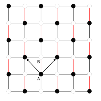
Figure 1: $\pi$-flux phase on a $6\times 6$ square lattice. Sublattices A and B are shown by solid and open circles. Bonds in red correspond to hopping $t^{\prime}=-t$, as opposite to black lines with hopping $t$. Arrows represent the basis vectors.

The two dimensional $\pi$-flux phase on a square lattice is schematically shown in Fig. 1. All hopping in the $x$ direction are $t$, while half of the hoppings along the $y$-direction are set to $t^{\prime}=t\,e^{i\pi}=-t$, where the phase $\pi$ in the hopping amplitude arises from the Peierls prescription for the vector potential of the magnetic field. As a consequence, an electron hopping on a contour around each plaquette picks up a total phase $\pi$, corresponding to one half of a magnetic flux quantum $\Phi_{0}=hc/e$ per plaquette. The lattice is bipartite, with two sublattices $A$ and $B$. Each unit cell consists of two sites. In reciprocal space, with the reduced Brillouin zone $(|k_{x}|\leq\pi,|k_{y}|\leq|k_{x}|)$, the non-interacting part of Hamiltonian Eq.(1) can be written as,

$$\mathcal{\hat{H}}_{0} =\sum_{\bf{k}\sigma}\hat{\psi}^{\dagger}_{\bf{k}\sigma}{\bf H}_{0}({\bf k})\hat{\psi}^{\phantom{\dagger}}_{\bf{k}\sigma},$$ (2)

where

$$\hat{\psi}_{\bf{k}\sigma}=\left(\begin{array}[]{cc}\hat{d}^{\phantom{\dagger}}_{A\sigma}&\hat{d}^{\phantom{\dagger}}_{B\sigma}\\ \end{array}\right)^{T},$$ (4)

and the noninteracting Hamiltonian matrix

$${\bf H}_{0}({\bf k})=\left(\begin{array}[]{cc}0&2\,t\,{\rm cos}k_{x}+2\,i\,t\,{\rm sin}k_{y}\\ 2\,t\,{\rm cos}k_{x}-2\,i\,t\,{\rm sin}k_{y}&0\\ \end{array}\right).$$ (7)

The energy spectrum $E_{\bf k}=\pm 2\,t\sqrt{\cos^{2}k_{x}+\sin^{2}k_{y}}$ describes a semi-metal with two inequivalent Dirac points at ${\bf K}_{\pm}=(\pm\pi/2,0)$, shown in Fig. 2. In the low-energy regime of the dispersion, the density of states (DOS) vanishes linearly near the Dirac point where $E_{\bf k}=0$, as shown in Fig. 3. The bandwidth of the $\pi$-flux phase is $W=4\sqrt{2}\,t$. In Fig. 3 the DOS of the honeycomb lattice is shown for comparison. The Dirac Fermi velocity is $v_{\rm F}=2t\ (1.5t)$ for the $\pi$-flux (honeycomb) lattice. Near the Dirac point, the DOS $\rho(\omega)\sim|\omega|/v_{\rm F}$, and the $\pi$-flux model has a smaller slope.

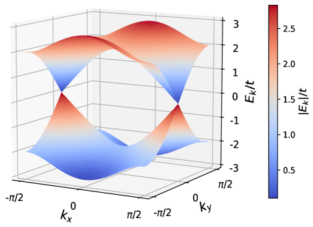
Figure 2: The dispersion relation $E_{\bf k}$ for $\pi$-flux phase on a square lattice. There are two Dirac points at $(k_{x},k_{y})=(\pm\pi/2,0)$. The bandwidth for the $\pi$-flux model is $W=4\sqrt{2}\,t$.

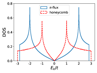
Figure 3: The density of states for the $\pi$-flux phase square lattice and the honeycomb lattice. The bandwidths are nearly identical, but the honeycomb lattice has a substantially larger slope of the linear increase of the DOS.

III III. Mean-Field Theory

In this section, we present a mean-field theory approach to solve the Holstein model. Semi-metal to superfluid transitions have previously been investigated with MFT in 2D and 3D Mazzucchi et al. (2013); Wu et al. (2014). Here we focus on the semi-metal to CDW transition. In the mean-field approximation, the phonon displacement at site ${\bf i}$ is replaced by its average value, modulated by a term which has opposite sign on the two sublattices,

$$\langle{X}_{\mathbf{i}}\rangle=X_{0}\pm X_{\rm mf}\,(-1)^{\bf i}\,\,.$$ (8)

Here $X_{0}=-\lambda/\omega_{0}^{2}$ is the “equilibrium position” at half-filling and $X_{\rm mf}$ is the mean-field order parameter. When $X_{\rm mf}$ = 0, phonons on all sites have the same average displacement, indicating the system remains in semi-metal phase, whereas when $X_{\rm mf}\neq 0$, the last term in the Hamiltonian Eq. (1), i.e., $\lambda\sum_{{\bf i},\sigma}\hat{n}_{{\bf i},\sigma}\hat{X}_{\bf i}$, becomes an on-site staggered potential, which corresponds to the CDW phase. The phonon kinetic energy term is zero as a result of the static field. The resulting static mean-field Hamiltonian is quadratic in the fermion operators. Diagonalizing gives energy eigenvalues $\epsilon_{n}(X_{\rm mf})$. The free energy $F$ can then be directly obtained by,

$$F(\beta,X_{\rm mf})=-\frac{1}{\beta}\sum_{n}{\rm ln}(1+e^{-\beta\epsilon_{n}})$$

$$+\frac{N\omega_{0}^{2}}{2}(X_{0}^{2}+X_{\rm mf}^{2}),$$ (9)

Minimizing the free energy with respect to $X_{\rm mf}$ (or equivalently, a self-consistent calculation) will determine the order parameter. $X_{\rm mf}$ is found to be zero at high temperatures: the energy cost of the second term in Eq. 9 exceeds the energy decrease in the first term associated with opening of a gap in the spectrum $\epsilon_{n}$. $X_{\rm mf}$ becomes nonzero below a critical temperature $T_{c}$.

$T_{c}$ for the $\pi$-flux lattice is shown in Fig. 4, along with the result of analogous MFT calculations for the honeycomb and (zero flux) square geometries. The lattice size $\rm L=180$ is chosen for all three models. This is sufficiently large so that finite size effects are smaller than the statistical sampling error bars. At zero temperature, the CDW order exhibits a critical EPC for the $\pi$-flux and the honeycomb lattices. This QCP arises from the Dirac fermion dispersion, which has a vanishing DOS at the Fermi energy. The honeycomb lattice QCP has a smaller critical value. However, when measured in units of the Fermi velocity, the ratios $\lambda_{D,{\rm crit}}/v_{\rm F}=0.13$ and $0.14$ are quite close for the honeycomb and $\pi$-flux geometries respectively. We will see this is also the case for the exact DQMC calculations. For the square lattice, on the other hand, the DOS has a Van-Hove singularity at the Fermi energy, and the CDW develops at arbitrarily small coupling strength.

Another feature of the MFT phase diagram is that, as the coupling increases, $T_{c}$ increases monotonically. This is in contrast to the exact DQMC results, where $T_{c}$ decreases at large coupling strengths (Fig. 13). A similar failure of MFT is well known for the Hubbard Hamiltonian where the formation of AF ordering is related to two factors: the local moment $m^{2}_{z}=(n_{\uparrow}-n_{\downarrow})^{2}=1-2\langle n_{\uparrow}n_{\downarrow}\rangle$ and the exchange coupling $J\sim t^{2}/U$. The double occupancy $\langle n_{\uparrow}n_{\downarrow}\rangle$ is suppressed by the interaction, resulting in the growth of the local moment. Thus upon cooling, the Hubbard model has two characteristic temperatures: the temperature of local moment formation, which increases monotonically with $U$, and further the AF ordering scale, which falls as $J$. Since the interaction is simply decoupled locally and the exchange coupling is not addressed, within MFT the formation of the local moments, and their ordering, occur simultaneously. MFT thus predicts a monotonically increasing $T_{c}$ with $U$.

Figure 4: MFT $T_{c}$ for CDW phase transition as a function of dimensionless coupling $\lambda_{D}$ for the square lattice with no magnetic flux, the $\pi$-flux phase square lattice, and the honeycomb lattice. For the geometries with a Dirac spectrum MFT captures the existence for a QCP, a critical value of $\lambda_{D}$ below which there is no CDW order even at $T=0$, and the absence of a QCP for the conventional square lattice.

IV IV. DQMC Methodology

We next describe the DQMC methodBlankenbecler et al. (1981); White et al. (1989). In evaluating the partition function $\mathcal{Z}$, the inverse temperature $\beta$ is discretized as $\beta=L_{\tau}\Delta\tau$, and complete sets of phonon position eigenstates are introduced between each $e^{-\Delta\tau{\cal\hat{H}}}$. The phonon coordinates acquire an “imaginary time” index, converting the 2-dimensional quantum system to a (2+1) dimensional classical problem. After tracing out the fermion degrees of freedom, which appear only quadratically in the Holstein Hamiltonian, the partition function becomes

$$\mathcal{Z}=\int\mathcal{D}x_{\mathbf{i},l}\,e^{-\mathcal{S}_{ph}}\left[\det{\mathbf{M}(x_{\mathbf{i},l})}\right]^{2},$$ (10)

where the “phonon action” is

$$\mathcal{S}_{ph}=\Delta\tau\left[\frac{1}{2}\omega_{0}^{2}\sum_{\mathbf{i}}x_{\mathbf{i},l}^{2}+\frac{1}{2M}\sum_{\mathbf{i}}\left(\frac{x_{\mathbf{i},l+1}-x_{\mathbf{i},l}}{\Delta\tau}\right)^{2}\right]\,.$$ (11)

Because the spin up and spin down fermions have an identical coupling to the phonon field, the fermion determinants which result from the trace are the same, and the determinant is squared in Eq. 10. Thus there is no fermion sign problemLoh et al. (1990). We use $\Delta\tau=0.1/t$, small enough so that Trotter errors associated with the discretization of $\beta$ are of the same order of magnitude as the statistical uncertainty from the Monte Carlo sampling.

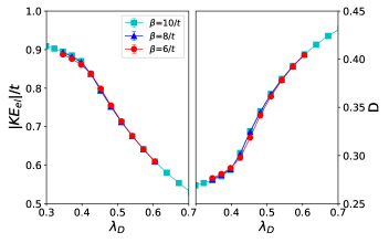
Figure 5: Left: The magnitude of electron kinetic energy $|\mathcal{K}_{\rm el}|$ as a function of EPC strength $\lambda_{D}$. Simulations are performed on a $\rm L=10$ lattice at inverse temperatures $\beta=6/t,8/t,10/t$ and fixed $\omega_{0}=1.0\,t$. Right: Double occupancy $D$ as a function of EPC strength $\lambda_{D}$.

V V. DQMC Results

V.1 Double occupancy and Kinetic Energy

We first show data for several local observables, the electron kinetic energy $|\mathcal{K}_{\rm el}|=|\sum_{\langle\mathbf{i},\mathbf{j}\rangle,\sigma}\big{(}t^{\phantom{\dagger}}_{\mathbf{i},\mathbf{j}}\,\hat{d}^{\dagger}_{\mathbf{i}\sigma}\hat{d}^{\phantom{\dagger}}_{\mathbf{j}\sigma}+{\rm h.c.}\big{)}|$ and double occupancy $\mathcal{D}=\langle\,n_{{\bf i}\uparrow}n_{{\bf i}\downarrow}\,\rangle$. For a tight-binding model on a bipartite lattice at half-filling, Lieb has shown that the energy-minimizing magnetic flux is $\pi$ per plaquette, both in for noninteracting fermions and in the presence of a Hubbard $U$ Lieb (1994). Here we show $|\mathcal{K}_{\rm el}|$ for the Holstein model, a case not hitherto considered.

Figure 5 shows $|\mathcal{K}_{\rm el}|$ (left panel) and $\mathcal{D}$ (right panel) as functions of the dimensionless EPC $\lambda_{D}$ for $\beta=6/t,8/t,10/t$. There is little temperature dependence for these local quantities. The magnitude of the kinetic energy $|\mathcal{K}_{\rm el}|$ decreases as $\lambda_{D}$ grows, reflecting the gradual localization of the dressed electrons (“polarons”).

At the same time, the double occupancy $\mathcal{D}$ evolves from its noninteracting value $\mathcal{D}=\langle\,n_{{\bf i}\uparrow}n_{{\bf i}\downarrow}\,\rangle=\langle\,n_{{\bf i}\uparrow}\,\rangle\,\langle\,n_{{\bf i}\downarrow}\,\rangle=1/4$ at half-filling, to $\mathcal{D}=1/2$ at large $\lambda_{D}$. In the strong coupling regime, we expect robust pair formation, so that half of the lattice sites will be empty and half will be doubly occupied.

The evolution of $\mathcal{D}$ and $|\mathcal{K}_{\rm el}|$ have largest slope at $\lambda_{D}\sim 0.42$ which, as will be seen, coincides with the location of the QCP between the semi-metal and CDW phases.

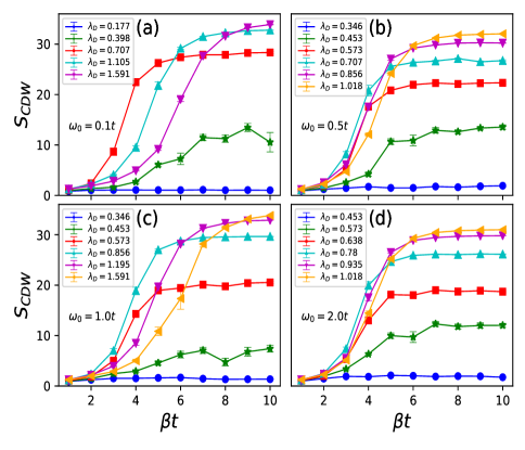
Figure 6: The CDW structure factor of the $\pi$-flux phase Holstein model as a function of inverse temperature $\beta$. The phonon frequencies $\omega_{0}$ are (a), $0.1\,t$; (b), $0.5\,t$; (c), $1.0\,t$; (d), $2.0\,t$ in the four panels. The lattice size $L=6$.

V.2 Existence of Long-Range CDW Order

The structure factor $S({\bf Q})$ is the Fourier transform of the real-space spin-spin correlation function $c({\bf r})$,

$$S(\bf Q) =\sum_{\bf r}e^{i\bf Q\cdot\bf r}c({\bf r}),$$

$$c({\bf r}) =\big{\langle}\,\big{(}\,n_{{\bf i}\uparrow}+n_{{\bf i}\downarrow}\,\big{)}\big{(}\,n_{{\bf i+r}\uparrow}+n_{{\bf i+r}\downarrow}\,\big{)}\,\big{\rangle},$$ (12)

and characterizes the charge ordering. In a disordered phase $c({\bf r})$ is short-ranged and $S({\bf Q})$ is independent of lattice size. In an ordered phase, $c({\bf r})$ remains large out to long distances, and the structure factor will be proportional to the number of sites, at the appropriate ordering wave vector ${\bf Q}$. At half-filling $S({\bf Q})$ is largest at ${\bf Q}=(\pi,\pi)$. We define $S_{\rm cdw}\equiv S(\pi,\pi)$. Figure 6 displays $S_{\rm cdw}$ as a function of inverse temperature $\beta$ at different phonon frequencies $\omega_{0}$ and coupling strengths $\lambda_{D}$. The linear lattice size $L=6$. At fixed $\omega_{0}$ and strong coupling, $S_{\rm cdw}$ grows as temperature is lowered, and saturates to $S_{\rm cdw}\sim\rm N$, indicating the development of long-range order (LRO), i.e. the phase transition into CDW phase. Note that $\beta=10/t$ is always in the plateau region, suggesting the correlation length has become larger than the lattice size, and the ground state has been reached. In the following, we use $\beta=10/t$ to represent the properties at $T\rightarrow 0$.

However, as $\lambda_{D}$ is decreased sufficiently, $S_{\rm cdw}$ eventually shows no signal of LRO even at large $\beta$, providing an indication that there is a QCP, with CDW order only occurring above a finite $\lambda_{D}$ value. Figure 6 also suggests that the critical temperature $T_{c}$ is non-monotonic with increasing $\lambda_{D}$. The values of $\beta$ at which $S_{\rm cdw}$ grows first shift downward, but then become larger again. This non-monotonicity agrees with previous studies of Dirac fermions on the honeycomb lattice Zhang et al. (2019); Chen et al. (2019). We can estimate the maximum $T_{c}$ to occur at $\lambda_{D}\approx 0.71,0.71,0.86$ and $0.78$ for $\omega_{0}=0.1\,t,0.5\,t,1.0\,t,2.0\,t$ respectively. In the anti-adiabatic limit $\omega_{0}\rightarrow\infty$, the Holstein model maps onto the attractive Hubbard model, and $T_{c}=0$ owing to the degeneracy of CDW and superconducting correlationsScalettar et al. (1989). (The order parameter has a continuous symmetry.) A recent studyFeng et al. (2020) has shown that $\omega_{0}\gtrsim 10^{2}\,t$ is required to achieve the $-U$ Hubbard model limit, a surprisingly large value.

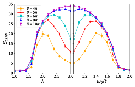
Figure 7: $S_{\rm cdw}$ (a) as a function of $\lambda$ at fixed $\omega_{0}=1.0\,t$; and (b) as a function of $\omega_{0}$ at fixed $\lambda$=3.0, at different inverse temperatures $\beta$. Lattice size $L=6$ is used in this figure.

Figure 7(a) shows $S_{\rm cdw}$ as a function of $\lambda$ at fixed $\omega_{0}=1.0\,t$. At the highest temperature shown, $\beta=4/t$, $S_{\rm cdw}$ reaches maximum at intermediate coupling $\lambda\sim 2.0$, then decreases as $\lambda$ gets larger. The region for which $S_{\rm cdw}$ is large is a measure of the range of $\lambda$ for which the CDW ordering temperature $T_{c}$ exceeds $\beta^{-1}$. As $\beta$ increases, this range is enlarged. Figure 7(b) is an analogous plot of $S_{\rm cdw}$ as a function of $\omega_{0}$ at fixed $\lambda=3.0$. The two plots appear as mirror images of each other since the dimensionless EPC $\lambda_{D}=\lambda^{2}/(\omega_{0}^{2}W)$ increases with $\lambda$, but decreases with $\omega_{0}$.

It is interesting to ascertain the extent to which the physics of the Holstein Hamiltonian is determined by $\lambda$ and $\omega_{0}$ separately, versus only the combination $\lambda_{D}$. Figure 8 addresses this issue by replotting the data of Figs. 7(a,b) as a function of $\lambda_{D}$ for two values of the inverse temperature. For $\lambda_{D}\gtrsim 0.8$, the data collapse well, whereas at small $\lambda_{D}$ $S_{\rm cdw}$ can vary by as much as a factor of two even though $\lambda_{D}$ is identical. It is likely that this sensitivity to the individual values of $\lambda$ and $\omega_{0}$ is associated with proximity to the QCP.

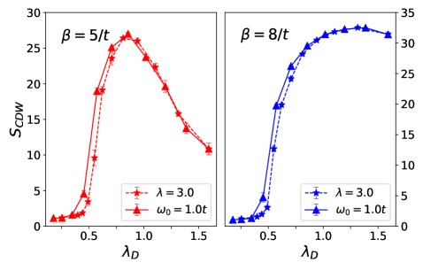
Figure 8: Comparison of the evolution of $S_{\rm cdw}$ with coupling strength by changing $\lambda$ or changing $\omega_{0}$. Data are taken from Fig. 7(a,b), for $\beta=5/t$ (left) and $\beta=8/t$ (right). The difference is negligible at $\lambda_{D}>0.8$ but not in the coupling regime $0.4<\lambda_{D}<0.8$ near the QCP.

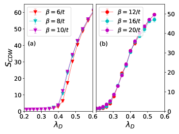
Figure 9: $S_{\rm cdw}$ as a function of $\lambda_{D}$ for $\pi$-flux phase square lattice (left) and honeycomb model (right). The lattice size $L=6$ is used for both geometries. $\lambda_{D}$ is varied by changing $\lambda$ at fixed $\omega_{0}=1.0\,t$. $S_{\rm cdw}$ does not change for the lowest temperatures, indicating that the ground state has been reached for this finite lattice size.

We compare the semi-metal to CDW transition with increasing $\lambda_{D}$ for the $\pi$-flux phase and honeycomb lattices in Fig. 9. These data are at lower temperatures than those of Fig. 8, so that the ground state values of $S_{\rm cdw}$ have been reached for the system sizes shown.

V.3 Ground State in the ($\lambda,\omega_{0}$) Plane

Figure 10 provides another perspective on the dependence of the CDW order on $\lambda$ and $\omega_{0}$ individually, by giving a heat map of $S_{\rm cdw}$ in the ($\lambda,\omega_{0}$) plane at low temperature. The bright yellow in upper-left indicates a strong CDW phase, whereas the dark purple region in lower-right indicates the Dirac semi-metal phase. The phase boundary is roughly linear, as would be expected if only the combination $\lambda_{D}=\lambda^{2}/(\omega_{0}^{2}W)$ is relevant. We note, however, that this statement is only qualitatively true. The more precise line graphs of Fig. 8 indicate that along the line $\lambda=\sqrt{\lambda_{D,{\rm crit}}W}\,\omega_{0}\sim 1.5\,\omega_{0}$, the separate values of $\lambda$ and $\omega_{0}$ are relevant.

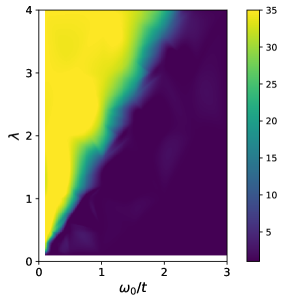
Figure 10: Heat map of the ground state values of $S_{\rm cdw}$ in the ($\lambda,\omega_{0}$) plane.

V.4 Finite Size Scaling: Finite $T$ Transition

A quantitative determination of the finite temperature and quantum critical points can be done with finite size scaling (FSS). Figure 11 gives both raw and scaled data for $S_{\rm cdw}$ for different lattice sizes $L=4,6,8,10$ at $\lambda=2.0$, $\omega_{0}=1.0\,t$ as a function of $\beta$. Unscaled data are in panel (a): $S_{\rm cdw}$ is small and $L$-independent at small $\beta$ (high $T$) where $c({\bf r})$ is short ranged. On the other hand, $S_{\rm cdw}$ is proportional to $N=L^{2}$ at large $\beta$ (low $T$), reflecting the long-range CDW order in $c({\bf r})$. Panel (b) shows a data crossing for different $L$ occurs when $S_{\rm cdw}/L^{\gamma/\nu}$ is plotted versus $\beta$. A universal crossing is seen at $\beta\,t\sim 3.80\pm 0.02$, giving a precise determination of critical temperature $T_{c}$. The 2D Ising critical exponents $\gamma=7/4$ and $\nu=1$ were used in this analysis, since the CDW phase transition breaks a similar discrete symmetry. Panel (c) shows a full data collapse when the $\beta$ axis is also appropriately scaled by $L^{1/\nu}$. The best collapse occurs at $\beta_{c}=3.80/t$, consistent with the result from the data crossing.

In the region immeditely above the QCP, the DQMC values for $T_{c}$ are roughly five times lower than those obtained in MFT, and, indeed, the MFT over-estimation of $T_{c}$ can be made arbitrarily large at strong coupling. This reflects both the relatively low dimensionality ($d=2$) and the fact that MFT fails to distinguish moment-forming and moment-ordering temperature scales.

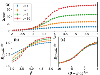
Figure 11: (a) The CDW structure factor $S_{\rm cdw}$ as a function of $\beta$ for several lattice sizes. (b) The scaled CDW structure factor $S_{\rm cdw}/\mathrm{L}^{\gamma/\nu}$ as a function of $\beta$ using Ising critical exponents $\gamma=7/4$ and $\nu=1$, showing a crossing of different L at $\beta_{c}=3.80/t$. (c) $S_{\rm CDW}/\mathrm{L}^{\gamma/\nu}$ versus $(\beta-\beta_{c})\rm L$, giving a best data collapse at $\beta_{c}=3.80/t$. Here the parameters are $\lambda=2.0$ and $\omega_{0}=1.0\,t$.

V.5 Quantum Phase Transition

Analysis of the renormalization group invariant Binder cumulant(Binder, 1981),

$$\mathcal{B}=\frac{3}{2}\left(1-\frac{1}{3}\frac{<S_{\rm cdw}^{2}>}{<S_{\rm cdw}>^{2}}\right),$$ (13)

can be used to locate the quantum critical point precisely. Only lattice sizes $L=4n$ where $n$ is an integer can be used, for other $L$ the Dirac points are not one of the allowed ${\bf k}$ values and finite size effects are much more significant. As exhibited in Fig. 12, for $L=4,8$ and $12$, $\mathcal{B}$ exhibits a set of crossings in a range about $\lambda_{D}\approx 0.4$. An extrapolation in $1/L$, as shown in the inset of Fig. 12, gives $\lambda_{D,{\rm crit}}=0.371\pm 0.003$.

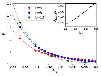
Figure 12: Main panel: Binder cumulant as a function of EPC strength $\lambda_{D}$ for three lattice sizes. Inverse temperature is $\beta=2\,L$ and $\omega_{0}$ is fixed at $\omega_{0}=1.0\,t$. Inset: Extrapolation of the crossings for pairs of sizes as a function of $1/L$ to get the QCP in the thermodynamic limit.

V.6 Phase Diagram

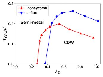
Figure 13: Critical temperature $T_{c}$ for CDW phase transition, obtained from DQMC for both $\pi$-flux phase square lattice (blue line) and the honeycomb lattice (red line), in a range of coupling strength. $\lambda_{D}$ is varied by changing $\lambda$ at fixed $\omega_{0}=1.0\,t$ for both models. Quantum critical point is determined using Binder cumulant analysis (discussed below). Data for the honeycomb lattice are taken from (Zhang et al., 2019) Error bars are smaller than symbol size for $\pi$-flux data.

Location of the finite temperature phase boundary, Fig. 11, and the QCP, Fig. 12, can be combined into the phase diagram of Fig. 13. Results for the $\pi$-flux geometry (blue circles) are put in better context by compared with those of the honeycomb lattice (red triangles). Data were obtained at fixed $\omega_{0}=1.0\,t$. In both geometries, phase transitions into CDW order happen only above a finite $\lambda_{D,{\rm crit}}$. Beyond $\lambda_{D,{\rm crit}}$, $T_{c}$ rises rapidly to its maximal value before decaying. For $\pi$-flux model, $T_{c}$ reaches a maximum $T_{c,{\rm max}}/t\sim 0.26$ at $\lambda_{D}\sim 0.7$, whereas for the honeycomb lattice $T_{c}$ reaches its maximum $T_{c,{\rm max}}/t\sim 0.20$ at $\lambda_{D}\sim 0.5$. Similarly $\lambda_{D,crit}$ for $\pi$-flux is larger than that of the honeycomb lattice, as $\lambda_{D,crit}=0.42$ and $0.27$ respectively. When measured in terms of the relative Fermi velocities $v_{\rm F}=2\,t,\,1.5\,t$ for the $\pi$-flux and honeycomb respectively, these values become very similar: $\lambda_{D,{\rm crit}}/v_{\rm F}=0.21$ and $0.18$ for $\pi$-flux and honeycomb; $T_{c,{\rm max}}/v_{\rm F}=0.13$ and $0.13$.

VI VI. Conclusions

This paper has determined the quantitative phase diagram for Dirac fermions interacting with local phonon modes on the $\pi$-flux lattice. A key feature, shared with the honeycomb geometry, is the presence of a quantum critical point $\lambda_{D,{\rm crit}}$ below which the system remains a semi-metal down to $T=0$. The values of $T_{c}$ and $\lambda_{D,{\rm crit}}$ for the two cases, when normalized to the Fermi velocities, agree to within roughly 10%.

We have also considered the question of whether the properties of the model can be described in terms of the single ratio $\lambda^{2}/\omega_{0}^{2}$. We find that qualitatively this is indeed the case, but that, quantititively, the charge structure factor can depend significantly on the individual values of EPC and phonon frequency, especially in the vicinity of the QCP. However this more complex behavior is masked by the fact that $T_{c}$ rises so rapidly with $\lambda$ in that region. In investigating this issue we have studied substantially smaller values of $\omega_{0}$ than have typically been investigated in QMC treatments of the Holstein Hamiltonian.

Acknowledgments: The work of Y.-X.Z. and R.T.S. was supported by the grant DE‐SC0014671 funded by the U.S. Department of Energy, Office of Science. H.G. was supported by NSFC grant No. 11774019. The authors would like to thank B. Cohen-Stead and W.-T. Chiu for useful conversations.

References

- Castro Neto et al. (2009) A. H. Castro Neto, F. Guinea, N. M. R. Peres, K. S. Novoselov, and A. K. Geim, “The electronic properties of graphene,” Rev. Mod. Phys. 81, 109–162 (2009).
- Geim (2009) A.K. Geim, “Graphene: Status and prospects,” Science 324, 1530 (2009).
- Choi et al. (2010) Wonbong Choi, Indranil Lahiri, Raghunandan Seelaboyina, and Yong Soo Kang, “Synthesis of graphene and its applications: A review,” Crit. Rev. in Solid State and Mat. Sci. 35, 52–71 (2010).
- Novoselov et al. (2012) Konstantin S Novoselov, VI Fal, L Colombo, PR Gellert, MG Schwab, K Kim, et al., “A roadmap for graphene,” nature 490, 192–200 (2012).
- Harris et al. (1989) A Brooks Harris, Tom C Lubensky, and Eugene J Mele, “Flux phases in two-dimensional tight-binding models,” Phys. Rev. B 40, 2631 (1989).
- Jia et al. (2013) Yongfei Jia, Huaiming Guo, Ziyu Chen, Shun-Qing Shen, and Shiping Feng, “Effect of interactions on two-dimensional dirac fermions,” Phys. Rev. B 88, 075101 (2013).
- Otsuka and Hatsugai (2002) Y. Otsuka and Y. Hatsugai, “Mott transition in the two-dimensional flux phase,” Phys. Rev. B 65, 073101 (2002).
- Otsuka et al. (2014) Yuichi Otsuka, Seiji Yunoki, and Sandro Sorella, “Mott transition in the 2d hubbard model with -flux,” in Proceedings of the International Conference on Strongly Correlated Electron Systems (SCES2013) (2014) p. 013021.
- Li et al. (2015) Zi-Xiang Li, Yi-Fan Jiang, and Hong Yao, “Fermion-sign-free majarana-quantum-monte-carlo studies of quantum critical phenomena of dirac fermions in two dimensions,” New J. of Phys. 17, 085003 (2015).
- Toldin et al. (2015) Francesco Parisen Toldin, Martin Hohenadler, Fakher F Assaad, and Igor F Herbut, “Fermionic quantum criticality in honeycomb and -flux hubbard models: Finite-size scaling of renormalization-group-invariant observables from quantum monte carlo,” Phys. Rev. B 91, 165108 (2015).
- Otsuka et al. (2016) Yuichi Otsuka, Seiji Yunoki, and Sandro Sorella, “Universal quantum criticality in the metal-insulator transition of two-dimensional interacting dirac electrons,” Phys. Rev. X 6, 011029 (2016).
- Lang and Läuchli (2019) Thomas C. Lang and Andreas M. Läuchli, “Quantum monte carlo simulation of the chiral heisenberg gross-neveu-yukawa phase transition with a single dirac cone,” Phys. Rev. Lett. 123, 137602 (2019).
- Guo et al. (2018a) H-M Guo, Lei Wang, and RT Scalettar, “Quantum phase transitions of multispecies dirac fermions,” Phys. Rev. B 97, 235152 (2018a).
- Guo et al. (2018b) Huaiming Guo, Ehsan Khatami, Yao Wang, Thomas P Devereaux, Rajiv RP Singh, and Richard T Scalettar, “Unconventional pairing symmetry of interacting dirac fermions on a -flux lattice,” Phys. Rev. B 97, 155146 (2018b).
- Wang et al. (2014) Lei Wang, Philippe Corboz, and Matthias Troyer, “Fermionic quantum critical point of spinless fermions on a honeycomb lattice,” New J. of Phys. 16, 103008 (2014).
- Meng et al. (2010) Z.Y. Meng, T.C. Lang, S. Wessel, F.F. Assaad, and A. Muramatsu, “Quantum spin liquid emerging in two-dimensional correlated dirac fermions,” Nature 464, 847–851 (2010).
- Otsuka et al. (2013) Y. Otsuka, S. Yunoki, and S. Sorella, “Quantum monte carlo study of the half-filled hubbard model on the honeycomb lattice,” J. of Phys.: Conf. Series 454, 012045 (2013).
- Zhou et al. (2018) Zhichao Zhou, Congjun Wu, and Yu Wang, “Mott transition in the -flux hubbard model on a square lattice,” Phys. Rev. B 97, 195122 (2018).
- Chang and Scalettar (2012) Chia-Chen Chang and Richard T. Scalettar, “Quantum disordered phase near the mott transition in the staggered-flux hubbard model on a square lattice,” Phys. Rev. Lett. 109, 026404 (2012).
- Holstein (1959) T Holstein, “Studies of polaron motion: Part i. the molecular-crystal model,” Annals of Physics 8, 325 – 342 (1959).
- Kornilovitch (1998) P.E. Kornilovitch, “Continuous-time quantum monte carlo algorithm for the lattice polaron,” Phys. Rev. Lett. 81, 5382 (1998).
- Kornilovitch (1999) P. E. Kornilovitch, “Ground-state dispersion and density of states from path-integral monte carlo: Application to the lattice polaron,” Phys. Rev. B 60, 3237–3243 (1999).
- Alexandrov (2000) A. S. Alexandrov, “Polaron dynamics and bipolaron condensation in cuprates,” Phys. Rev. B 61, 12315–12327 (2000).
- Hohenadler et al. (2004) M. Hohenadler, H. G. Evertz, and W. von der Linden, “Quantum monte carlo and variational approaches to the holstein model,” Phys. Rev. B 69, 024301 (2004).
- Ku et al. (2002) Li-Chung Ku, S. A. Trugman, and J. Bonča, “Dimensionality effects on the holstein polaron,” Phys. Rev. B 65, 174306 (2002).
- Spencer et al. (2005) P. E. Spencer, J. H. Samson, P. E. Kornilovitch, and A. S. Alexandrov, “Effect of electron-phonon interaction range on lattice polaron dynamics: A continuous-time quantum monte carlo study,” Phys. Rev. B 71, 184310 (2005).
- Macridin et al. (2004) A. Macridin, G. A. Sawatzky, and Mark Jarrell, “Two-dimensional hubbard-holstein bipolaron,” Phys. Rev. B 69, 245111 (2004).
- Romero et al. (1999) Aldo H. Romero, David W. Brown, and Katja Lindenberg, “Effects of dimensionality and anisotropy on the holstein polaron,” Phys. Rev. B 60, 14080–14091 (1999).
- Scalettar et al. (1989) R. T. Scalettar, N. E. Bickers, and D. J. Scalapino, “Competition of pairing and peierls˘charge-density-wave correlations in a two-dimensional electron-phonon model,” Phys. Rev. B 40, 197–200 (1989).
- Marsiglio (1990) F Marsiglio, “Pairing and charge-density-wave correlations in the holstein model at half-filling,” Physical Review B 42, 2416 (1990).
- Vekic et al. (1992) M. Vekic, R.M. Noack, and S.R. White, “Charge-density waves versus superconductivity in the holstein model with next-nearest-neighbor hopping,” Phys. Rev. B 46, 271 (1992).
- Niyaz et al. (1993) Parhat Niyaz, J. E. Gubernatis, R. T. Scalettar, and C. Y. Fong, “Charge-density-wave-gap formation in the two-dimensional holstein model at half-filling,” Phys. Rev. B 48, 16011–16022 (1993).
- Vekić and White (1993) M. Vekić and S. R. White, “Gap formation in the density of states for the holstein model,” Phys. Rev. B 48, 7643–7650 (1993).
- Freericks et al. (1993) JK Freericks, M Jarrell, and DJ Scalapino, “Holstein model in infinite dimensions,” Phys. Rev. B 48, 6302–6314 (1993).
- Zheng and Zhu (1997) H. Zheng and S. Y. Zhu, “Charge-density-wave and superconducting states in the holstein model on a square lattice,” Phys. Rev. B 55, 3803–3815 (1997).
- Jeckelmann et al. (1999) Eric Jeckelmann, Chunli Zhang, and Steven R. White, “Metal-insulator transition in the one-dimensional holstein model at half filling,” Phys. Rev. B 60, 7950–7955 (1999).
- Zhang et al. (2019) Y.-X. Zhang, W.-T. Chiu, N. C. Costa, G. G. Batrouni, and R. T. Scalettar, “Charge order in the holstein model on a honeycomb lattice,” Phys. Rev. Lett. 122, 077602 (2019).
- Chen et al. (2019) Chuang Chen, Xiao Yan Xu, Zi Yang Meng, and Martin Hohenadler, “Charge-density-wave transitions of dirac fermions coupled to phonons,” Phys. Rev. Lett. 122, 077601 (2019).
- Affleck and Marston (1988) Ian Affleck and J Brad Marston, “Large-n limit of the heisenberg-hubbard model: Implications for high-t c superconductors,” Physical Review B 37, 3774 (1988).
- Aidelsburger et al. (2011) Monika Aidelsburger, Marcos Atala, Sylvain Nascimbene, Stefan Trotzky, Y-A Chen, and Immanuel Bloch, “Experimental realization of strong effective magnetic fields in an optical lattice,” Physical review letters 107, 255301 (2011).
- Gazit et al. (2017) Snir Gazit, Mohit Randeria, and Ashvin Vishwanath, “Emergent dirac fermions and broken symmetries in confined and deconfined phases of z 2 gauge theories,” Nature Physics 13, 484–490 (2017).
- Lieb (1994) Elliott H. Lieb, “Flux phase of the half-filled band,” Phys. Rev. Lett. 73, 2158–2161 (1994).
- Mazzucchi et al. (2013) Gabriel Mazzucchi, Luca Lepori, and Andrea Trombettoni, “Semimetal–superfluid quantum phase transitions in 2d and 3d lattices with dirac points,” J. of Phys,. B: Atomic, Mol. and Opt. Phys. 46, 134014 (2013).
- Wu et al. (2014) Ya-Jie Wu, Jiang Zhou, and Su-Peng Kou, “Strongly fluctuating fermionic superfluid in the attractive -flux hubbard model,” Phys. Rev. A 89, 013619 (2014).
- Blankenbecler et al. (1981) R. Blankenbecler, D. J. Scalapino, and R. L. Sugar, “Monte carlo calculations of coupled boson-fermion systems. i,” Phys. Rev. D 24, 2278–2286 (1981).
- White et al. (1989) S. R. White, D. J. Scalapino, R. L. Sugar, E. Y. Loh, J. E. Gubernatis, and R. T. Scalettar, “Numerical study of the two-dimensional hubbard model,” Phys. Rev. B 40, 506–516 (1989).
- Loh et al. (1990) E. Y. Loh, J. E. Gubernatis, R. T. Scalettar, S. R. White, D. J. Scalapino, and R. L. Sugar, “Sign problem in the numerical simulation of many-electron systems,” Phys. Rev. B 41, 9301–9307 (1990).
- Feng et al. (2020) Chunhan Feng, Huaiming Guo, and Richard T Scalettar, “Charge density waves on a half-filled decorated honeycomb lattice,” Physical Review B 101, 205103 (2020).
- Binder (1981) Kurt Binder, “Finite size scaling analysis of ising model block distribution functions,” Zeitschrift für Physik B Condensed Matter 43, 119–140 (1981).