Asteroid Diameters and Albedos from NEOWISE Reactivation Mission Years Four and Five

Abstract

The Near-Earth Object Wide-field Infrared Survey Explorer (NEOWISE) spacecraft has been conducting a two-band thermal infrared survey to detect and characterize asteroids and comets since its reactivation in Dec 2013. Using the observations collected during the fourth and fifth years of the survey, our automated pipeline detected candidate moving objects which were verified and reported to the Minor Planet Center. Using these detections, we perform thermal modeling of each object from the near-Earth object and Main Belt asteroid populations to constrain their sizes. We present thermal model fits of asteroid diameters for $189$ NEOs and $5831$ MBAs detected during the fourth year of the survey, and $185$ NEOs and $5776$ MBAs from the fifth year. To date, the NEOWISE Reactivation survey has provided thermal model characterization for $957$ unique NEOs. Including all phases of the original WISE survey brings the total to $1473$ unique NEOs that have been characterized between 2010 and the present.

1 Introduction

The Near Earth Object Wide-field Infrared Survey Explorer (NEOWISE, Mainzer et al., 2014b) has been continuously surveying the sky since 13 Dec 2013. NEOWISE utilizes the Wide-field Infrared Survey Explorer (WISE, Wright et al., 2010) satellite that was reactivated to discover and characterize near-Earth asteroids in an effort to quantify the risk they pose to Earth. All NEOWISE images and extracted source data from the first five years of the Reactivation survey are publicly accessible via the NASA/IPAC Infrared Science Archive (IRSA). The content and characteristics of NEOWISE data are described in Cutri et al. (2015).

Observations of NEOs offer us the opportunity to study the smallest asteroids as they pass close to the Earth, when they are significantly easier to see. These objects, having escaped from the Main Belt or the Jupiter-family comet populations (e.g. Bottke et al., 2002; Granvik et al., 2018), let us probe the physics of the formation and evolution of sub-kilometer-sized bodies. NEOs also represent a potential hazard to Earth, and thus survey and characterization of them enables us to better quantify the chances of impact and the dangers these objects pose.

The NEOWISE team has previously published the thermal modeling results from the first three years of the Reactivation survey in Nugent et al. (2015, 2016); Masiero et al. (2017). These fits, along with those from previous survey phases, have been archived in the NASA Planetary Data System (Mainzer et al., 2019). Here, we perform the same analysis on the data collected during the survey’s fourth and fifth years (13 Dec 2016 to 12 Dec 2017, and 13 Dec 2017 to 12 Dec 2018, respectively). At the end of the NEOWISE reactivated survey, all asteroid thermal modeling results will be delivered to the NASA Planetary Data System, to augment the current archive from the original phases of the WISE mission and the first three years of the NEOWISE Reactivation survey currently archived there. The current mission plan is to operate through June 2020, however the slower-than-expected evolution of the spacecraft’s orbit may allow for further useful survey lifetime, which is currently being evaluated.

2 Observations

NEOWISE scans the sky along lines of constant ecliptic longitude, recording images every 11 seconds, as the spacecraft orbits the Earth in a 94-minute polar orbit. The spacecraft was originally launched onto a terminator-following orbit. Since then, as expected, the orbit has gradually precessed off of the terminator to an average offset of $\sim 18-22^{\circ}$ during the survey’s fourth and fifth years. On the evening side of the orbit the spacecraft continues to survey at the zenith point with respect to Earth, and thus at larger Solar elongations, but on the morning side the telescope cannot point closer to the Sun and therefore must maintain a pointing at Solar elongation of $\sim 90^{\circ}$, away from the local zenith point. This off-zenith pointing results in an increase in the heat load on the telescope from the Earth that gradually raises the telescope temperature over time. As in the past, NEOWISE continues to toggle its scan circles to avoid the Moon, speeding and slowing the progression of the survey to avoid directly scanning over it. NEOWISE collects $\sim 12$ detections per moving object over a span of $\sim 30$ hours for objects near the ecliptic. Objects closer to the ecliptic poles can follow the survey region for long periods of time resulting in longer sets of observations, while objects near the detection limit may be detected fewer times as noise and light curve variations shift them below the cutoff level.

Over the course of six months as the Earth orbits the Sun, NEOWISE obtains images of the entire inertial sky. As NEOs often have similar orbits to the Earth, and thus long synodic periods, objects previously undetected by NEOWISE regularly pass through the survey’s field of regard. NEOWISE employs the WISE Moving Object Processing System (WMOPS, Mainzer et al., 2011a) to perform regular searches of the survey data for new and known moving Solar System objects. This is done initially without incorporating any knowledge about the previous discovery status of an object, enabling us to use the recovery of previously known objects as a test of the efficiency of discovering new ones (see Mainzer et al., 2011c). WMOPS is run three times per week, and all tracklets verified by our quality assurance process are submitted to the Minor Planet Center (MPC) for publication and archiving.

WMOPS requires a minimum of 5 detections at a signal-to-noise ratio of SNR$>4.5$, and has been shown to have an efficiency of $85\%-90\%$ for bright objects within our selection requirements on number of detections and motion vectors(Mainzer et al., 2011c). However, there are some objects that are observed but will be missed due to low SNR, or because they were moving too quickly through the field of regard and were not seen a sufficient number of times, or because they had highly curved motions on the plane of the sky that violate our linearity-of-motion requirements for tracklet linking (a velocity difference of 0.01 deg/day or a velocity angle change of 1 degree between pairs of detections, which typically span 3 hours). Searches for known near-Earth objects found by other surveys with detections not identified by WMOPS were carried out for the cryogenic WISE mission data (Mainzer et al., 2014a) and the first three years of the NEOWISE reactived survey data (Masiero et al., 2018a), recovering detections of $105$ and $116$ NEOs not found by WMOPS, respectively. A similar search of the NEOWISE Reactivation Years 4 and 5 data is underway and will be presented in future work.

The NEOWISE telescope uses a beamsplitter to collect images simultaneously in the $3.4~{}\mu$m (W1) and $4.6~{}\mu$m (W2) bandpasses. For objects with heliocentric distances near 1 AU, W2 is generally dominated by thermal emission while W1 can be thermally dominated or a mixture of thermal emission and reflected light depending on the temperature of the object and how reflective the object is at $3.4~{}\mu$m. For more distant objects, e.g. Main Belt asteroids (MBAs), W1 is almost always dominated by reflected light and W2 can range from thermally-dominated to reflected-light-dominated depending on the object’s distance from the Sun and $4.6~{}\mu$m reflectivity. As a result, for the majority of detected NEOs we have sufficient information to perform basic thermal modeling using simplifying assumptions to reduce the number of variable parameters (such as assuming the value for the beaming parameter and ratio of the infrared albedo to the visible albedo). For MBAs, conversely, only about half of the objects detected had sufficient thermal emission to allow thermal modeling to set a constraint on the diameter. The remaining objects, which had significant contributions of reflected light to both NEOWISE bandpasses, are not included in the subsequent analysis. Astrometric detections of them are still recorded in the Minor Planet Center’s database.

For more details on the survey and telescope, refer to the NEOWISE Explanatory Supplement (Cutri et al., 2015), which is updated for each annual NEOWISE data release.

3 Thermal Modeling Technique

The measured thermal flux from an asteroid depends on the object’s temperature, observing geometry, and size. When enough astrometric measurements are available to allow for the orbit to be constrained, the distances to the Sun, Earth, and spacecraft as well as the phase angle at the time of observation will be sufficiently well-known to contribute negligible error to the final thermal model fit. Thus, by employing a model of the thermal properties of the surface, along with the known observational geometries, the diameter of the asteroid can be constrained based on the measured flux in the thermally dominated bands. Using optical measurements from the literature (in particular, the absolute $H$ magnitude published along with the orbital information) the albedo of the asteroid can also be constrained, however the uncertainty on this value depends on the uncertainties on the diameter and the $H$ magnitude (cf. Masiero et al., 2018b).

3.1 Data

The process for data extraction follows the same method used in Masiero et al. (2017). To extract the data for use in thermal fitting, we refer to the Minor Planet Center’s Observations Catalog, which contains all observations of asteroids and comets submitted by NEOWISE (observatory code C51) that were vetted and published by the MPC. We extracted all observations from C51 within survey Year 4 and Year 5. By using the MPC-accepted observations, we have a data set that has initial source rejection done by the WMOPS pipeline as well as subsequent checks on positional offsets by MPC that can flag the occasional observation that was contaminated by cosmic rays or other artifacts. To obtain the fluxes associated with each detection reported to the MPC we use the position-time measurements as an input for the search of the NEOWISE Single-Exposure source database hosted by IRSA, conducting a search for extracted sources within 5 arcsec of the position and 5 secs of the MJD reported to the MPC.

NEOWISE source detection and photometry is carried out using the expected PSF at that location on each detector simultaneously (Cutri et al., 2015). The quality of the fit between the PSF and the identified source is recorded as a reduced $\chi^{2}$ value for each bandpass. We performed a filtering on the detections prior to using them for thermal modeling based on their reduced $\chi^{2}$ of the fit of the model PSF to the W2 detection (parameter $w2rchi2$), removing any detection with $w2rchi2>5$. This cut removes detections that may be contaminated by cosmic rays or other spurious noise that could potentially bias the fitted diameter. We also remove from consideration any object with an orbital arc shorter than 0.01 years, as these objects received little-to-no ground based followup and thus have uncertain orbits which will result in potentially incorrect distance calculations and thermal modeling results. This last cut removed 3 NEOs and 15 MBAs from the Year 4 observation list, and 9 MBAs from the Year 5 list (no NEOs were removed by this cut in Year 5). Future recovery of these objects by other telescopes would enable orbit fitting and thermal modeling, however at the moment the current orbital knowledge is insufficient.

To constrain the optical albedos for objects as part of our thermal modeling, we use the photometric $H_{V}$ absolute magnitude and $G$ slope parameter provided by the Minor Planet Center. When available, we updated the H-G parameters using the values published by Vereš et al. (2015) from the Pan-STARRS survey for objects that had phase coverage $>1^{\circ}$ in those data (cf. Masiero et al., 2017, for discussion on the effects of using these values). As these values are based on a single, well-calibrated photometric system, they offer some improvement over the values used by the MPC which incorporate a number of different surveys with different levels of photometric calibration. When not otherwise provided, we assume an uncertainty on $H$ of $0.05~{}$mag for the Main Belt and $0.2~{}$ mag for the NEOs, and an uncertainty on $G$ of $0.1$ based on our previous thermal modeling experience. As our sample of detected MBAs is primarily low-numbered objects with long orbital arcs, the small assumed uncertainty on $H$ is appropriate. Assuming a larger uncertainty on $H$ for MBAs can allow a reflected light measurement in W1 to dominate the least-squares fitting of that component of the model, and result in poor matches to the published $H$ magnitude in some cases.

3.2 NEATM

For our fitting, we employ the Near-Earth Asteroid Thermal Model (NEATM, Harris, 1998). This model provides a simple description of the behavior of temperature across the surface of a spherical asteroid, making use of a “beaming parameter” $\eta$ to consolidate uncertainties in the assumed values of the physical properties and differences between the model and actual temperature distribution. Extreme values in the beaming parameter can also provide indications of potentially unusual composition (cf. Harris & Drube, 2014). In all cases, we used an assumed value for the beaming parameter based on the distribution of fitted beaming values from the cryogenic NEOWISE mission (Mainzer et al., 2011c; Masiero et al., 2011). For NEOs we assume $\eta=1.4\pm 0.5$, while for MBAs we assume $\eta=0.95\pm 0.2$. This $1~{}\sigma$ uncertainty is used when conducting our Monte Carlo analysis to propagate to the final uncertainty on the fitted parameters diameter and albedo and is assumed to be normally distributed around the mean value.

We note that in previous analyses (e.g. Nugent et al., 2015, 2016; Masiero et al., 2017) we allowed beaming to be a fitted parameter for some NEOs where our observations indicated they were likely to be thermally dominated in both W1 and W2 bands. For this work, our thermal modeling code was updated to Python 3. Comparison of the output between the two versions shows that in the vast majority of cases ($98.6\%$) the software converges to identical solutions within the expected precision of the numerical routines. In a few cases when beaming was allowed to vary, the different code versions could settle to distinct solutions. This is because subtle differences in initial conditions result in slightly different estimates for the fraction of flux in W1 that is due to thermal emission, which would then change whether the code allowed beaming to vary or not. It is important to note that in these cases our Monte Carlo error analysis correctly captured the uncertainty on the diameter solutions. The different diameters were well within the large resulting uncertainties. As these are edge cases that straddle fixed/fitted decision point in the code, and we have no independent method of determining if beaming should be fitted or fixed, for the current analysis we hold beaming fixed in all cases.

Previous work (Mainzer et al., 2012; Masiero et al., 2012; Nugent et al., 2015, 2016; Masiero et al., 2017) has shown that the characteristic $1\sigma$ diameter uncertainty for the population of objects observed with W1 and W2 and fit with NEATM is $\sim 20\%$. More detailed thermophysical models, which constrain physical surface properties, can be used to perform multi-epoch fits which can potentially offer improved diameter constraints when a range of viewing geometries is available (e.g. Alí-Lagoa et al., 2014; Hanuš et al., 2016). However, these models take many orders of magnitude longer to run, and are not likely to return improved results compared to the NEATM unless observations covering a wide range of phase and distances are available. Further, these models require knowledge of the spin period and pole direction, or sufficient data to fit those parameters, which are not present for the majority of asteroids that have limited infrared and/or visible coverage. As such, we provide NEATM fits to all detected objects with sufficient data to better understand the larger population and identify objects that may be of interest for more detailed modeling in the future.

Our fitting procedure follows the method used in previous work (e.g. Masiero et al., 2017). In summary, each photometric observation from NEOWISE acts as a measurement to be fit by the Python least-squares fitting routine in the scipy package(Jones et al., 2019). Observations include the position, time, magnitudes and uncertainties in W1 and W2, and spacecraft positions. We require that an object have at least 3 measurements with magnitude uncertainty $<0.25~{}$mag (SNR$~{}\sim 4$) in a WISE band for it to be used in fitting. We only use an additional band for fitting if the number of detections is more than $40\%$ of the number in the band with the largest number of detections. This requirement is designed to remove potential contamination from cosmic rays and background objects that may have been missed by other filters. It also results in a requirement that there are at least 3 detections for a second band to be used in the minimum case of a 5-detection tracklet (the lower limit produced by WMOPS). The published $H$ and $G$ visible photometric parameters are also included as a measurement to be fitted by the least-squares fitter. The asteroid’s orbit is used to determine Sun-to-object and object-to-spacecraft distances as well as phase angle at each observation time, which is used by NEATM to determine the temperature distribution across the surface. Specifically, we use a faceted sphere made up of 288 facets in bands spaced at 15 degrees in latitude and calculate the temperature on each facet as well as the resulting emission that would be observed.

Reflected light at visible wavelengths is constrained by the $H$ magnitude measurement. To constrain the reflected light in the NEOWISE bandpasses, we assume a ratio of albedos between the infrared and visible of $1.5\pm 0.5$ for MBAs and $1.6\pm 1.0$ for NEOs, based on the best fit values found during the cryogenic WISE mission for objects where these parameters were fitted (Mainzer et al., 2011c; Masiero et al., 2011). (These are different because the NEO population is not a random sample of the MBAs, but over-represents asteroids from the $\nu_{6}$ region.) In cases where the W1 band is dominated by reflected light and has a very high SNR, the assumed infrared-to-visible albedo ratio can result in the least-squares minimizer finding a best fit solution where the predicted $H$ magnitude (based on the fitted diameter and optical albedo) does not match the measured value exactly. Fits with large deviations between the model and measured $H$ magnitudes are checked to ensure the solutions are physically plausible. In addition, fits with visible albedos below $p_{V}<0.01$ or above $p_{V}=0.9$ are also checked. Previous work (see Masiero et al., 2017) found that the majority of fits producing nonphysical or otherwise suspect results occurred when more than $10\%$ of the flux in W2 was contributed by reflected light based on best-fit parameters. Following that work, we discard these fits as unreliable, and do not include them in our final tables.

The statistical uncertainty on each fitted parameter is determined by performing 25 Monte Carlo trials, using uncertainties on each measurement and the estimated uncertainties for assumed parameters. Each trial draws a new value from a normal distribution around the measured or assumed parameter, and conducts a least-squares fit to those parameters. The standard deviation of the population of all Monte Carlo model fitted parameters is then taken as the $1\sigma$ uncertainty. These quoted uncertainties will only represent the statistical component of the model fit, and do not account for systematic offsets of the NEATM model with respect to reality.

4 Results

We present our model fits for NEOs and MBAs observed during Year 4 in Table 1 and Table 2 respectively. Fits for NEOs and MBAs observed during Year 5 are given in Tables 3 and 4 respectively. Year 4 contains $214$ fits of $189$ unique NEOs, and $6658$ fits of $5831$ unique MBAs. Year 5 contains $215$ fits for $185$ unique NEOs, and $6600$ fits of $5776$ unique MBAs. Each table gives the object’s name (in MPC-packed format), the measured $H$ and $G$ values used in the process of fitting, the number of observations used in W1 and W2, the orbital phase angle at the midpoint of the observations, along with the best-fit diameter, the visible albedo, and beaming parameter, with their associated uncertainties. As we held beaming fixed for all fits in this work, the beaming flag in the tables are all set to $0$, but the flag is retained for easy comparison to previously published results. For objects that were seen at multiple epochs in a given year, we present each fit as a separate entry in the tables. For objects that have non-spherical shapes, different epochs can help constrain the true spherical equivalent diameter instead of the projection-dependent results from a single epoch. Alternately, different epochs can provide insight into the thermal behavior of the surface. Thus, different diameter constraints from different epochs of observation could be due to changing physical parameters, or simply be a result of statistical noise.

We note that one object in the Year 5 NEO table, 2018 KK₂, has a best-fit albedo $p_{V}<0.01$ despite our attempts at filtering or changing assumed parameters. This Amor-class NEO has an orbital arc spanning $\sim 3$ months with observations that span $\sim 10^{\circ}$ of phase, however the scatter in the photometry means that the published $H$ value is not necessarily well-constrained (see Figure 1). The NEOWISE observations of this object occurred at a phase of $\alpha=30^{\circ}$, so a poorly constrained G value won’t have as large an effect on the predicted brightness at the time of our observations. An underestimated brightness from an $H$ value that was too large would drive the albedo to artificially low values. The unphysically low albedo is then likely the result of a combination of poor $H$ fit and statistical uncertainty on the size measurement, possibly combined with light curve variations. We include the best fit as reported by our model in the results table. While the diameter should be reliable to the quoted errors, caution should be used regarding the interpretation of the albedo for this object. This highlights the impact that uncertainty on the optical measurements has on our ability to determine albedos, and shows the need for improved $H$ and $G$ determinations for all objects from a photometrically calibrated survey (e.g. Jurić et al., 2002; Vereš et al., 2015).

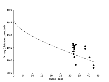
Figure 1: Distance-corrected magnitude measurements for asteroid 2018 KK₂ from the Minor Planet Center observation database are shown with black points. The dashed line is the expected photometric behavior of an object with $H=18.4$ and $G=0.15$. Magnitudes were converted from the observed G and R bands assuming Solar colors of $V-R=0.36$ and $G-V=-0.14$ (Ramírez et al., 2012, Gaia Data Release Documentation (http://gea.esac.esa.int/archive/documentation/GDR2/)), compatible with a flat-spectral slope expected for low-albedo C-type objects.

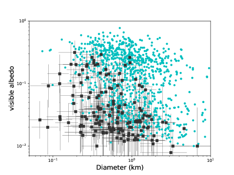
Figure 2: Comparison of fitted diameters and albedos for all near-Earth objects observed (cyan circles) and discovered (black squares) by NEOWISE during the first five years of the reactivation survey (Dec 2013 to Dec 2018) by the WMOPS pipeline. The majority of objects discovered by NEOWISE tend to have albedos below $10\%$ and diameters larger than a few hundred meters, filling in a region of phase space missed by other surveys (cf. Mainzer et al., 2011c, figure 14). Error bars on previously known objects are omitted for clarity, but are of comparable size to the uncertainties on the NEOWISE discoveries.

We show a plot of diameter and albedo for all near-Earth objects detected by NEOWISE from Dec 2013 to Dec 2018 in Figure 2. Objects discovered by NEOWISE show a preference for being low albedo, with many of them being larger than $200~{}$m in diameter. This population of objects is more likely to be missed by the visible light ground-based surveys due to albedo-dependent selection effects inherent in those systems. Thus, while NEOWISE is primarily a NEO-characterization mission, it fills an important part of phase space in the current suite of near-Earth object discovery surveys.

Table 1: Thermal model fits for NEOs detected in the fourth year of the NEOWISE survey. Table 1 is published in its entirety in the electronic edition; a portion is shown here for guidance regarding its form and content.

Name	H†	G	Diameter	$p_{V}^{\dagger\dagger}$	beaming†††	nW1	nW2	phase	Fitted
	(mag)		(km)					(deg)	Beaming?
01864	14.85	0.15	2.73 $\pm$ 0.79	0.271 (+0.205/-0.117)	1.40 $\pm$ 0.50	5	5	54.84	0
02102	16.00	0.15	1.53 $\pm$ 0.56	0.298 (+0.257/-0.138)	1.40 $\pm$ 0.50	8	8	58.12	0
02329	14.50	0.15	4.17 $\pm$ 1.72	0.148 (+0.147/-0.074)	1.40 $\pm$ 0.50	12	12	38.45	0
03122	14.10	0.15	4.21 $\pm$ 1.12	0.351 (+0.234/-0.140)	1.40 $\pm$ 0.50	19	19	79.28	0
03122	14.10	0.15	4.28 $\pm$ 1.27	0.346 (+0.237/-0.141)	1.40 $\pm$ 0.50	33	33	73.15	0
03352	15.80	0.15	1.55 $\pm$ 0.43	0.274 (+0.203/-0.117)	1.40 $\pm$ 0.50	17	18	50.01	0
03752	15.30	0.15	2.48 $\pm$ 0.92	0.238 (+0.208/-0.111)	1.40 $\pm$ 0.50	14	16	48.65	0
04179	15.30	0.10	2.64 $\pm$ 1.05	0.254 (+0.240/-0.123)	1.40 $\pm$ 0.50	10	10	61.09	0
04197	14.60	0.15	3.67 $\pm$ 1.47	0.155 (+0.149/-0.076)	1.40 $\pm$ 0.50	5	5	58.95	0
05653	16.20	0.15	1.60 $\pm$ 0.63	0.261 (+0.246/-0.127)	1.40 $\pm$ 0.50	21	24	50.25	0

^†Measured H used as input for the modeling; the model-output H value can be found using the output diameter, albedo, and the equation $D=1329*10^{H/-5}/\sqrt{p_{V}}$
^††Albedo uncertainties are symmetric in log-space as the error is dominated by the uncertainty on $H$; the asymmetric linear equivalents of the $1\sigma$ log-space uncertainties are presented here.
^†††Assumed constant value; not fit.

Table 2: Thermal model fits for MBAs detected in the fourth year of the NEOWISE survey. Table 2 is published in its entirety in the electronic edition; a portion is shown here for guidance regarding its form and content.

Name	H†	G	Diameter	$p_{V}^{\dagger\dagger}$	beaming†††	nW1	nW2	phase	Fitted
	(mag)		(km)					(deg)	Beaming?
00010	5.43	0.15	438.31 $\pm$ 144.12	0.046 (+0.072/-0.028)	0.95 $\pm$ 0.20	7	8	20.83	0
00013	6.74	0.15	197.47 $\pm$ 59.09	0.057 (+0.039/-0.023)	0.95 $\pm$ 0.20	7	7	23.90	0
00019	7.13	0.10	227.74 $\pm$ 68.19	0.034 (+0.024/-0.014)	0.95 $\pm$ 0.20	4	5	25.65	0
00025	7.83	0.15	97.99 $\pm$ 18.06	0.196 (+0.080/-0.057)	0.95 $\pm$ 0.20	10	10	29.82	0
00031	6.74	0.15	302.09 $\pm$ 113.80	0.035 (+0.032/-0.017)	0.95 $\pm$ 0.20	10	10	23.70	0
00034	8.51	0.15	116.40 $\pm$ 47.83	0.038 (+0.037/-0.019)	0.95 $\pm$ 0.20	10	10	22.26	0
00046	8.36	0.06	124.71 $\pm$ 28.64	0.052 (+0.044/-0.024)	0.95 $\pm$ 0.20	8	8	21.88	0
00050	9.24	0.15	87.30 $\pm$ 30.40	0.035 (+0.028/-0.016)	0.95 $\pm$ 0.20	6	9	29.67	0
00051	7.35	0.08	134.63 $\pm$ 36.55	0.090 (+0.055/-0.034)	0.95 $\pm$ 0.20	13	13	25.93	0
00051	7.35	0.08	128.44 $\pm$ 31.02	0.087 (+0.051/-0.032)	0.95 $\pm$ 0.20	12	12	22.62	0

^†Measured H used as input for the modeling; the model-output H value can be found using the output diameter, albedo, and the equation $D=1329*10^{H/-5}/\sqrt{p_{V}}$
^††Albedo uncertainties are symmetric in log-space as the error is dominated by the uncertainty on $H$; the asymmetric linear equivalents of the $1\sigma$ log-space uncertainties are presented here.
^†††Assumed constant value; not fit.

Table 3: Thermal model fits for NEOs detected in the fifth year of the NEOWISE survey. Table 3 is published in its entirety in the electronic edition; a portion is shown here for guidance regarding its form and content.

Name	H†	G	Diameter	$p_{V}^{\dagger\dagger}$	beaming†††	nW1	nW2	phase	Fitted
	(mag)		(km)					(deg)	Beaming?
00719	15.50	0.15	2.59 $\pm$ 0.81	0.189 (+0.175/-0.091)	1.40 $\pm$ 0.50	16	16	46.48	0
01627	13.20	0.60	8.99 $\pm$ 3.31	0.129 (+0.112/-0.060)	1.40 $\pm$ 0.50	23	23	41.56	0
01627	13.20	0.60	9.01 $\pm$ 2.36	0.127 (+0.075/-0.047)	1.40 $\pm$ 0.50	25	27	52.18	0
01627	13.20	0.60	5.96 $\pm$ 1.98	0.167 (+0.130/-0.073)	1.40 $\pm$ 0.50	7	7	54.86	0
01916	14.93	0.15	2.77 $\pm$ 1.07	0.212 (+0.217/-0.107)	1.40 $\pm$ 0.50	8	8	43.30	0
03552	12.90	0.15	26.89 $\pm$ 12.58	0.028 (+0.032/-0.015)	1.40 $\pm$ 0.50	12	13	35.31	0
04596	16.30	0.15	2.10 $\pm$ 0.74	0.173 (+0.144/-0.079)	1.40 $\pm$ 0.50	11	11	45.89	0
05797	18.70	0.15	0.45 $\pm$ 0.16	0.288 (+0.274/-0.141)	1.40 $\pm$ 0.50	0	7	48.69	0
09856	17.40	0.15	0.91 $\pm$ 0.39	0.245 (+0.258/-0.125)	1.40 $\pm$ 0.50	8	8	66.67	0
09856	17.40	0.15	0.94 $\pm$ 0.35	0.252 (+0.221/-0.118)	1.40 $\pm$ 0.50	8	8	53.74	0

^†Measured H used as input for the modeling; the model-output H value can be found using the output diameter, albedo, and the equation $D=1329*10^{H/-5}/\sqrt{p_{V}}$
^††Albedo uncertainties are symmetric in log-space as the error is dominated by the uncertainty on $H$; the asymmetric linear equivalents of the $1\sigma$ log-space uncertainties are presented here.
^†††Assumed constant value; not fit.

Table 4: Thermal model fits for MBAs detected in the fifth year of the NEOWISE survey. Table 4 is published in its entirety in the electronic edition; a portion is shown here for guidance regarding its form and content.

Name	H†	G	Diameter	$p_{V}^{\dagger\dagger}$	beaming†††	nW1	nW2	phase	Fitted
	(mag)		(km)					(deg)	Beaming?
00013	6.74	0.15	219.07 $\pm$ 78.46	0.053 (+0.045/-0.024)	0.95 $\pm$ 0.20	9	9	20.42	0
00013	6.74	0.15	235.06 $\pm$ 73.14	0.047 (+0.037/-0.021)	0.95 $\pm$ 0.20	5	5	22.57	0
00019	7.13	0.10	190.24 $\pm$ 57.83	0.057 (+0.042/-0.024)	0.95 $\pm$ 0.20	12	12	21.41	0
00034	8.51	0.15	105.98 $\pm$ 30.95	0.041 (+0.027/-0.016)	0.95 $\pm$ 0.20	9	10	23.85	0
00034	8.51	0.15	105.52 $\pm$ 30.53	0.042 (+0.044/-0.021)	0.95 $\pm$ 0.20	19	19	21.63	0
00038	8.32	0.15	87.36 $\pm$ 36.65	0.061 (+0.062/-0.031)	0.95 $\pm$ 0.20	9	10	23.89	0
00041	7.12	0.10	179.21 $\pm$ 56.70	0.053 (+0.043/-0.024)	0.95 $\pm$ 0.20	17	17	22.72	0
00045	7.46	0.07	138.44 $\pm$ 40.24	0.076 (+0.085/-0.040)	0.95 $\pm$ 0.20	11	11	21.47	0
00045	7.46	0.07	175.21 $\pm$ 44.60	0.058 (+0.058/-0.029)	0.95 $\pm$ 0.20	13	13	21.70	0
00046	8.36	0.06	118.09 $\pm$ 29.19	0.050 (+0.028/-0.018)	0.95 $\pm$ 0.20	3	4	29.06	0

^†Measured H used as input for the modeling; the model-output H value can be found using the output diameter, albedo, and the equation $D=1329*10^{H/-5}/\sqrt{p_{V}}$
^††Albedo uncertainties are symmetric in log-space as the error is dominated by the uncertainty on $H$; the asymmetric linear equivalents of the $1\sigma$ log-space uncertainties are presented here.
^†††Assumed constant value; not fit.

5 Accuracy of the NEATM Thermal Modeling

As discussed in Wright et al. (2019), the diameters derived by NEOWISE have a characteristic $1\sigma$ uncertainty in effective spherical diameter of $\sim 10\%$ for objects with sufficient data to fit multiple thermal bands. This was found through comparisons between diameter fits from NEOWISE and diameters determined by the IRAS satellite (Tedesco et al., 2004). Usui et al. (2014) found a similar result for comparisons between the cryogenic NEOWISE fits and AKARI. These works focused on data from the cryogenic mission, so an independent check of the fits based on 2-band Reactivation data is appropriate. We show the comparison between the NEOWISE Reactivation survey years 4 and 5 diameters and the diameters from the IRAS and AKARI data (for objects with more than 5 detections to reduce selection effect biases) in Figure 3.

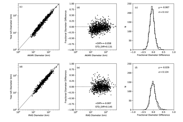
Figure 3: Main Belt asteroid diameter fits from the NEOWISE Reactivation Years 4 and 5 data compared to diameters derived from AKARI measurements (Usui et al., 2014, panel (a)) and IRAS (Tedesco et al., 2004, panel (d)). Dotted lines show a 1:1 relationship. We show the fractional difference in fits against the comparison diameter ((year 4/5 - comparison)/comparison; panels (b) and (e)) for each comparison set. We also show the histogram of the fractional differences (panels (c) and (f)) along with the best-fit Gaussian to the fractional difference distribution and its mean ($\mu$) and standard deviation ($\sigma$).

To additionally verify the diameters published here, we perform a comparison of the Years 4 and 5 fits to previously published results. For these comparisons, we use three primary datasets: a collection of published radar reflection sizes (Hudson & Ostro, 1994; Magri et al., 1999; Shevchenko & Tedesco, 2006; Magri et al., 2007; Shepard et al., 2010; Naidu et al., 2015) and occultation timing chords (D̆urech et al., 2011; Herald et al., 2019); diameters from the fully cryogenic NEOWISE dataset which had fitted beaming parameters; and diameters from the NEOWISE Reactivation Years 1-3. NEOWISE diameters are drawn from the compilation in the NASA Planetary Data System (Version 2, Mainzer et al., 2019).

Figure 4 shows the comparison between the Main Belt asteroid fits published here with previously published values, while Figure 5 shows the near-Earth objects. For the Main Belt population we find that the best-fit Gaussian to the diameter deviations for the population shows $1\sigma$ spreads of $11-17\%$ with systematic offsets of no more than a few percent. The comparison to the NEOWISE cryogenic diameters shows a $\sim 5\%$ offset for the population, with a comparable offset seen in the AKARI and IRAS comparisons. This offset is not seen in the comparison to the earlier NEOWISE reactivation diameters, so indicates a shift between the cryogenic and reactivation fits. This offset, however, is within the $10\%$ minimum systematic uncertainty we assume for our implementation of our thermal model (Mainzer et al., 2011b).

A few objects in our comparison of Main Belt sizes show large deviations between the thermal modeled diameter and the size measured by occultations (Herald et al., 2019), with the thermal diameter being much larger. The largest outliers in our comparison are (90) Antiope [81 vs 127 km], (415) Palatia [55 vs 98 km], and (431) Nephele [68 vs 112 and 121 km at two different epochs]. All of these agree well with diameters obtained through thermal modeling in other epochs of NEOWISE (Mainzer et al., 2019). For Antiope, the occultation diameter is the size of the primary only of the equal-mass binary, so the difference from size when assuming a single sphere (as we do in our diameter calculation) is understood. Palatia is a lower-confidence (U=2) occultation, so not covered completely by chords. For Nephele, the chord coverage looks sufficient to constrain the full shape, so this perhaps is another case of an equal-mass binary where only one component was picked up by the occultations.

The near-Earth population shows a larger Gaussian spread of $\sim 20-30\%$, but uses fewer comparison objects because the NEO population is smaller, and due to changing viewing geometry objects are not as likely to be re-detected at different epochs. This larger spread for the NEOs may be an indication that the population is more non-spherical than MBAs, or may simply be due to a combination of statistical noise and the limitations of the NEATM model at high phase angles, as discussed by Mommert et al. (2018). We do not fit a Gaussian to the comparison between NEOs and non-infrared diameter sources due to the small number of measurements in this dataset ($N=8$).

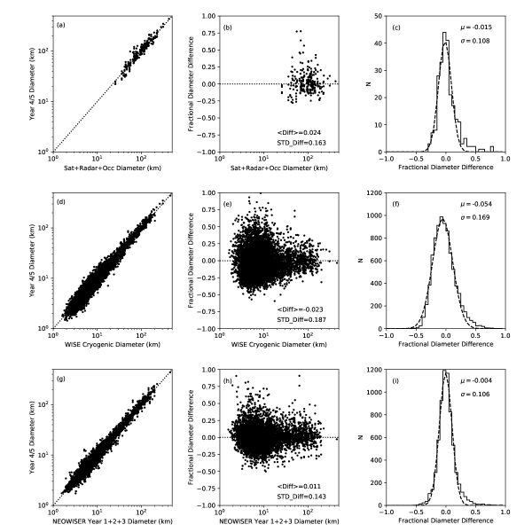
Figure 4: Main Belt asteroid diameter fits from the NEOWISE Reactivation Years 4 and 5 data compared to diameters derived from radar and occultation measurements (panel (a)), NEOWISE fully cryogenic data (panel (d)), and NEOWISE Reactivation Years 1-3 data (panel(g)). Dotted lines show a 1:1 relationship. We show the fractional difference in fits against the comparison diameter ((year 4/5 - comparison)/comparison; panels (b), (e), (h)) for each comparison set. We also show the histogram of the fractional differences (panels (c), (f), (i)) along with the best-fit Gaussian to the fractional difference distribution and its mean ($\mu$) and standard deviation ($\sigma$).

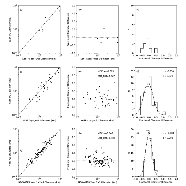
Figure 5: The same as Figure 4, but for near-Earth objects observed during Years 4 and 5 that also were present in the comparison datasets.

6 Conclusions

We present thermal model fits to near-Earth objects and Main Belt asteroids detected during the fourth and fifth years of the reactivated NEOWISE survey. Included are $214$ fits of $189$ unique NEOs and $6658$ fits of $5831$ MBAs from Year 4, and $215$ fits of $185$ unique NEOs and $6600$ fits of $5776$ MBAs from Year 5. We follow the data quality restrictions used for the fits to the NEOWISE Year 3 data (Masiero et al., 2017), in particular rejecting fits with $>10\%$ modeled reflected light in the W2 band as unstable solutions. This results in a large number of detected MBAs being rejected from the thermal fit results, but improves the fit reliability. This cut will introduce a strong bias against high albedo objects in the list of Main Belt objects characterized.

We find that the diameter fits for Main Belt asteroids have a characteristic $1\sigma$ uncertainty of $\sim 15\%$ compared to other data sets (assuming a Gaussian distribution), while NEOs show a larger uncertainty of $\sim 20-30\%$, consistent with what we have found in previous years, though this is based on a smaller comparison set. Thus there is no apparent degradation in the quality of the NEOWISE data as the survey has continued.

NEOWISE has provided thermal model characterization of $957$ unique NEOs during the Reactivation mission, bringing the total number of NEOs characterized from all mission phases to $1473$, including NEOs detected automatically by our WMOPS pipeline and those recovered later using the IRSA moving object search tools. The NEOWISE survey continues into its sixth year of operation. The spacecraft has precessed from its original terminator-following orbit, though the rate of precession has been slower than expected due to the low levels of Solar activity in the last few years. Eventually this precession will force an end to the mission, though it is difficult to predict the exact timing of when data quality will diminish. NEOWISE data continue to provide an important resource for discovering and characterizing asteroids and comets.

References

- Alí-Lagoa et al. (2014) Alí-Lagoa, V., Lionni, L., Delbo, M., Gundlach, B., Blum, J., & Licandro, J. 2014, A&A, 561, 45.
- Bottke et al. (2002) Bottke, W.F., Morbidelli, A., Jedicke, R. et al., 2002, Icarus, 156, 399.
- Cutri et al. (2015) Cutri, R.M., Mainzer, A., Conrow, T., Masci, F., Bauer, J., et al., 2015, Explanatory Supplement to the NEOWISE Data Release Products, http://wise2.ipac.caltech.edu/docs/release/neowise/expsup
- Dunham et al. (2016) Dunham, D., Herald, D., Frappa, E., Hayamizu, T., Talbot, J., & Timerson, B. 2016, NASA Planetary Data System, EAR-A-3-RDR-OCCULTATIONS-V14.0.
- D̆urech et al. (2011) D̆urech, J., Kaasalainen, M., Herald, D., Dunham, D et al., 2011, Icarus, 214, 652.
- Granvik et al. (2018) Granvik, M., Morbidelli, A., Jedicke, R., et al., 2018, Icarus, 312, 181.
- Hanuš et al. (2016) Hanuš, J., Delbo’, M., D̆urech, J. & Alí-Lagoa, V., 2018, Icarus, 309, 297.
- Harris (1998) Harris, A.W., 1998, Icarus, 131, 291.
- Harris & Drube (2014) Harris, A.W. & Drube, L., 2014, ApJL, 785, 4.
- Herald et al. (2019) Herald, D., Frappa, E., Gault, D., Hayamizu, T., Kerr, S., Moore, J., and Giacchini, B., Asteroid Occultations V3.0. urn:nasa:pds:smallbodiesoccultations::3.0. NASA Planetary Data System, 2019.
- Hudson & Ostro (1994) Hudson, R.S. & Ostro, S.J., 1994, Science, 263, 940.
- Jones et al. (2019) Jones, E., Oliphant, E., Peterson, P., et al., SciPy: Open Source Scientific Tools for Python, 2001-, http://www.scipy.org/ [Online; accessed 2019-07-25].
- Jurić et al. (2002) Jurić, M., Ivezić, Ž, Lupton, R. et al., 2002, AJ, 124, 1776.
- Magri et al. (1999) Magri, C., Ostro, S., Rosema, K., Thomas, M., et al., 1999, Icarus, 140, 379.
- Magri et al. (2007) Magri, C., Nolan, M., Ostro, S. & Giorgini, J., 2007, Icarus, 186, 126.
- Mainzer et al. (2011a) Mainzer, A.K., Bauer, J.M., Grav, T., Masiero, J., et al., 2011a, ApJ, 731, 53.
- Mainzer et al. (2011b) Mainzer, A.K., Grav, T., Masiero, J., Bauer, J.M., et al., 2011b, ApJ, 736, 100.
- Mainzer et al. (2011c) Mainzer, A.K., Grav, T., Bauer, J.M., Masiero, J., et al., 2011c, ApJ, 743, 156.
- Mainzer et al. (2012) Mainzer, A.K., Grav, T., Masiero, J., Bauer, J.M., Cutri, R.M. et al., 2012, ApJL, 760, 12.
- Mainzer et al. (2014a) Mainzer, A.K., Bauer, J., Grav, T., Masiero, J., Cutri, R., et al., 2014a, ApJ, 784, 110.
- Mainzer et al. (2014b) Mainzer, A.K., Bauer, J., Grav, T., Cutri, R., Masiero, J., et al., 2014b, ApJ, 792, 30.
- Mainzer et al. (2019) Mainzer, A., Bauer, J., Cutri, R., Grav, T., Kramer, E., Masiero, J., Sonnett, S., and Wright, E., Eds., NEOWISE Diameters and Albedos V2.0. urn:nasa:pds:neowise_diameters_albedos::2.0. NASA Planetary Data System, 2019
- Masiero et al. (2011) Masiero, J.R, Mainzer, A.K., Grav, T., Bauer, J.M., et al., 2011, ApJ, 741, 68.
- Masiero et al. (2012) Masiero, J.R, Mainzer, A.K., Grav, T., Bauer, J.M., Cutri, R.M. et al., 2012, ApJL, 759, 8.
- Masiero et al. (2012) Masiero, J.R, Grav, T., Mainzer, A.K., Nugent, C., Bauer, J., Stevenson, R., Sonnett, S., 2014, ApJ, 791, 121.
- Masiero et al. (2017) Masiero, J.R, Nugent, C.R., Mainzer, A.K., Wright, E.L., et al.2017, AJ, 154, 168.
- Masiero et al. (2018a) Masiero, J.R, Redwing, E., Mainzer, A.K., et al.2018a, AJ, 156, 60.
- Masiero et al. (2018b) Masiero, J.R, Mainzer, A.K., Wright, E.L., et al.2018b, AJ, 156, 62.
- Mommert et al. (2018) Mommert, M., Jedicke, R., Trilling, D.E., 2018, AJ, 155, 74.
- Naidu et al. (2015) Naidu, S., Margot, J.L., Taylor, P.A., Nolan M. et al., 2015, AJ, 150, 54.
- Nugent et al. (2015) Nugent, C.R., Mainzer, A., Masiero, J., Bauer, J.M., Cutri, R.M. et al., 2015, ApJ, 814, 117.
- Nugent et al. (2016) Nugent, C.R., Mainzer, A., Bauer, J.M., Cutri, R.M., Kramer, E. et al., 2016, AJ, 152, 63.
- Ramírez et al. (2012) Ramírez, I., Michel, R., Sefako, R., et al., 2012, ApJ, 752, 5.
- Shepard et al. (2010) Shepard, M., Clark, B., Ockert-Bell, M., Nolan, M. et al., 2010, Icarus, 208, 221.
- Shevchenko & Tedesco (2006) Shevchenko, V.G. & Tedesco, E.F., 2006, Icarus, 184, 211.
- Tedesco et al. (2004) Tedesco, E.F., P.V. Noah, M. Noah, & S.D. Price, 2004, IRAS Minor Planet Survey. IRAS-A-FPA-3-RDR-IMPS-V6.0. NASA Planetary Data System.
- Usui et al. (2014) Usui, F., Hasegawa, S., Ishiguro, M. Müller, T. G., Ootsubo, T., 2014, PASJ, 66, 56.
- Vereš et al. (2015) Vereš, P., Jedicke, R., Fitzsimmons, A., Denneau, L., Granvik, M. et al., 2015, Icarus, 261, 34.
- Wright et al. (2010) Wright, E.L., Eisenhardt, P., Mainzer, A.K., Ressler, M.E., Cutri, R.M., et al., 2010, AJ, 140, 1868.
- Wright et al. (2019) Wright, E.L., Mainzer, A., Masiero, J., et al., 2019, Icarus, under review (arXiv:1811.01454).