Towards Query-Efficient Black-Box Adversary with Zeroth-Order Natural Gradient Descent

Abstract

Despite the great achievements of the modern deep neural networks (DNNs), the vulnerability/robustness of state-of-the-art DNNs raises security concerns in many application domains requiring high reliability. Various adversarial attacks are proposed to sabotage the learning performance of DNN models. Among those, the black-box adversarial attack methods have received special attentions owing to their practicality and simplicity. Black-box attacks usually prefer less queries in order to maintain stealthy and low costs. However, most of the current black-box attack methods adopt the first-order gradient descent method, which may come with certain deficiencies such as relatively slow convergence and high sensitivity to hyper-parameter settings. In this paper, we propose a zeroth-order natural gradient descent (ZO-NGD) method to design the adversarial attacks, which incorporates the zeroth-order gradient estimation technique catering to the black-box attack scenario and the second-order natural gradient descent to achieve higher query efficiency. The empirical evaluations on image classification datasets demonstrate that ZO-NGD can obtain significantly lower model query complexities compared with state-of-the-art attack methods.

Introduction

Modern technologies based on machine learning (ML) and specifically deep learning (DL), have achieved significant breakthroughs (?) in various applications. Deep neural network (DNN) serves as a fundamental component in artificial intelligence. However, despite the outstanding performance, many recent studies demonstrate that state-of-the-art DNNs in computer vision (?; ?), speech recognition (?; ?) and deep reinforcement learning (?) are vulnerable to adversarial examples (?), which add carefully designed imperceptible distortions to legitimate inputs aiming to mislead the DNNs at test time. This raises concerns of the DNN robustness in many applications with high reliability and dependability requirements.

With the recent exploration of adversarial attacks in image classification and objection detection, the vulnerability/robustness of DNNs has attracted ever-increasing attentions and efforts in the research field known as adversarial machine learning. A large amount of efforts have been devoted to: 1) designing adversarial perturbations in various ML applications (?; ?; ?; ?; ?); 2) security evaluation methodologies to systematically estimate the DNN robustness (?; ?); and 3) defense mechanisms against adversarial attacks (?; ?; ?; ?; ?; ?; ?). This work mainly investigates the first category to build the groundwork towards developing potential defensive measures in reliable ML.

However, most of preliminary studies on this topic focus on the white-box setting where the target DNN model is completely available to the attacker (?; ?; ?). More specifically, the adversary can compute the gradients of the output with respect to the input to identify the effect of perturbing certain input pixels, with complete knowledge about the DNN model’s internal structure, parameters and configurations. Despite the theoretical interest, it is unrealistic to adopt the white-box adversarial methods to attack practical black-box threat models (?), where the internal model states/configurations are not revealed to the attacker (e.g., Google Cloud Vision API). Instead, the adversary can only query the model by submitting inputs and obtain the corresponding model outputs of prediction probabilities when generating adversarial examples.

In the black-box adversarial setting, it is often the case that the less queries, the more efficient an attack becomes. Large amount of queries may be at the risk of exposing the adversary or high financial cost in the case where the query is charged per query. Notably, to date most of the white-box (?; ?) and black-box attacks (?; ?; ?) are based on first-order gradient descent methods. Different from the widely utilized first-order optimization, the application of second-order optimization (?) is less explored due to the large computation overhead, although it may achieve faster convergence rate. The work (?) adopts natural gradient descent (NGD) to train ResNet-50 on ImageNet in 35 epochs, demonstrating its great potentiality.

In this work, inspired by the superb convergence performance of NGD, we propose zeroth-order natural gradient descent (ZO-NGD), which incorporates the zeroth-order (ZO) method and the second-order NGD, to generate black-box adversarial examples in a query-efficient manner. The contributions of this work are summarized as follows:

+ Design of adversary attacks with NGD: To the best of our knowledge, we are the first to derive the Fisher information matrix (FIM) and adopt the second-order NGD method for adversarial attacks, which is different from other first-order-based white-box and black-box attack methods.

+ Co-optimization of zeroth-order and second-order methods: In the black-box setting, we incorporate the zeroth-order random gradient estimation to estimate the gradients which is not directly available, and leverage the second-order NGD to achieve high query-efficiency.

+ No additional queries to obtain the FIM: During the queries to estimate the gradients of the loss, with our design the Fisher information is a byproduct that are extracted and evaluated without requiring additional query complexity.

+ Scalability to high dimensional datasets: In NGD, it is computationally infeasible to compute and invert the FIM with billions of elements on large scale datasets like ImageNet. To address this problem, we propose a method to avoid the computation and inverse of the FIM and thus the computation complexity is at most the same as the input images, rather than its square (the dimension of the FIM).

Related Work

In adversarial ML, the black-box setting is more practical where the attacker can only query the target model by providing input images and receive the probability density output for the input.

Black-box Attack

Attack with gradient estimation

In the black-box setting, as the gradients are not directly available, gradient estimation methods via zeroth-order optimization (?; ?; ?) are proposed to estimate the gradients. The ZOO method (?) performs pixel-level gradient estimation first and then perform white-box C&W attack (?) with the estimated gradients. Despite its high success rate, it suffers from intensive computation and huge queries due to element-wise gradient estimation.

The more practical threat models are investigated in (?). New attack methods based on Natural Evolutionary Strategies (NES) and Monte Carlo approximation to estimate the gradients are developed to mislead ImageNet classifiers under more restrictive threat models. The work (?) further proposes to use the prior information including the time-dependent priors and data-dependent priors to enhance the query efficiency.

Different from the previous first-order-based methods, the work (?) exploits the second-order optimization to improve query efficiency. In general, they explore Hessian information in the parameter space while our work explores the Hessian information in the distribution space (aka information matrix). Particularly, our method obtains the Fisher information during the first-order information (gradients) estimation for free while the mentioned paper needs additional queries for Hessian-based second-order optimization.

Heuristic black-box attacks

In the transfer attack (?), the attacker first trains a surrogate model with data labeled by the target model. White-box attacks are applied to attack the surrogate model and the generated examples are transferred to attack the target model. However, it may suffer from low attack success rate due to the low similarity between the surrogate model and the target model.

The boundary method (?) utilizes a conceptually simple idea to decrease the distortion through random walks and find successful adversarial perturbations while staying on the misclassification boundary. However, it suffers from high computational complexity and lacks algorithmic convergence guarantees.

Second-order optimization

First-order gradient descent methods have been extensively used in various ML tasks. They are easy to implement and suitable for large-scale DL. But these methods come with well known deficiencies such as relatively-slow convergence and sensitivity to hyper-parameter settings. On the other hand, second-order optimization methods provide a elegant solution by selectively re-scaling the gradient with the curvature information (?). As a kind of second-order method, NGD proves to be Fisher efficient by using the FIM instead of the Hessian matrix (?; ?). But the large overhead to compute, store and invert the FIM may limit its application. To address this, Kronecker Factored Approximate Curvature (K-FAC) is proposed to train DNNs (?).

Problem Formulation

Threat Model: In this paper, we mainly investigate black-box adversarial attacks for image classification with DNNs. Different from the white-box setting which has fully access to the DNN model and its internal structures/parameters, the black-box setting constrains the information available to the adversary. The attacker can only query the model by providing an input image and obtain the DNN output score/probability of the input. The black-box setting is more consistent with the scenario of “machine-learning-deployed-as-a-service” like Google Cloud Vision API.

In the following, we first provide a general problem formulation for adversarial attack which can be adopted to either white-box or black-box settings. Then, an efficient solution is proposed for the black-box setting. We highlight that this method can be easily adopted to the white-box setting by using the exact gradients to achieve higher query efficiency.

Attack Model: Given a legitimate image $\mathbf{x}\in\mathbb{R}^{d}$ with its correct class label $t$, the objective is to design an optimal adversarial perturbation $\bm{\delta}\in\mathbb{R}^{d}$ so that the perturbed example $(\mathbf{x}+\bm{\delta})$ can lead to a misclassification by the DNN model trained on legitimate images. The DNN model would misclassify the adversarial example to another class $t^{\prime}\neq t$. $\bm{\delta}$ can be obtained by solving the following problem,

$$\displaystyle\operatorname*{\text{minimize}}_{\bm{\delta}\in\mathbb{S}}f(\mathbf{x}+\bm{\delta},t),$$ (1)

where $\mathbb{S}=\{\bm{\delta}|(\mathbf{x}+\bm{\delta})\in[0,1]^{d},~{}\|\bm{\delta}\|_{\infty}\leq\epsilon\}$ and $f(\mathbf{x}+\bm{\delta},t)$ denotes an attack loss incurred by misclassifying $(\mathbf{x}+\bm{\delta})$ to another class $t^{\prime}$. $\|\cdot\|_{\infty}$ denotes the $\ell_{\infty}$ norm. In problem (1), the constraints on $\mathbb{S}$ ensure that the perturbed noise $\bm{\delta}$ at each pixel (normalized to $[0,1]$) is imperceptible up to a predefined $\epsilon$-tolerant threshold.

Motivated by (?), the loss function $f(\bm{x},t)$ is expressed as

$$f(\mathbf{x}+\bm{\delta},t)\ =\ \max\{ \log p(t|\mathbf{x}+\bm{\delta})$$

$$-\max_{i\neq t}\{\log p(i|\mathbf{x}+\bm{\delta})\},-\kappa\},$$ (2)

where $p(i|\mathbf{x})$ denotes the model’s prediction score or probability of the $i$-th class for the input $\bm{x}$, and $\kappa$ is a confidence parameter usually set to zero. Basically, $f(\mathbf{x}+\bm{\delta},t)$ achieves its minimum value 0 if $p(t|\mathbf{x}+\bm{\delta})$ is smaller than $\max_{i\neq t}\log p(i|\mathbf{x}+\bm{\delta})$, indicating there is a label with higher probability than the correct label $t$ and thus a misclassification is achieved by adding the perturbation $\bm{\delta}$ to $\bm{x}$. In this paper, we mainly investigate the untargeted attack which does not specify the target misclassified label. The targeted attack can be easily implemented following nearly the same problem formulation and loss function with slight modifications (?; ?). We focus on the general formulation here and omit the targeted attack formulation.

Note that in Eq. (Problem Formulation), we use the log probability $\log p(i|\mathbf{x})$ instead of $p(i|\mathbf{x})$ because the output probability distribution tends to have one dominating class. The log operator is used to reduce the effect of the dominating class while it still preserves the probability order of all classes.

As most of the white-box attack methods rely on gradient descent methods, the unavailability of the gradients in black-box settings will limit their application. Gradient estimation methods (known as zeroth-order optimization) are applied to perform the normal projected first-order gradient descent process (?; ?) as follows,

$${{\bm{\delta}}_{k+1}}={\prod_{\mathbb{S}}}\left({{{\bm{\delta}}_{k}}-\lambda\hat{\nabla}f({{\bm{\delta}}_{k}})}\right),$$ (3)

where $\lambda$ is the learning rate and the $\prod_{\mathbb{S}}(\cdot)$ performs the projection onto the feasible set $\mathbb{S}$.

In the black-box setting, it is often the case that the query number is limited or high query efficiency is required by the adversary. The zeroth-order method tries to extract gradient information of the objective function and the first-order method is applied to minimize the loss due to its wide application in ML. However, the second-order information of the queries is not fully exploited. In this paper, we aim to take advantages of the model’s second-order information and propose a novel method named ZO-NGD optimization.

Zeroth-order Nature Gradient Descent

The proposed method is based on NGD (?) and ZO optimization (?). In the applications of optimizing probabilistic models, NGD uses the natural gradient by multiplying the gradient with the FIM to update the parameters. NGD seems to be a potentially attractive alternative method as it requires fewer total iterations than gradient descent (?; ?; ?).

Motivated from the perspective of information geometry, NGD defines the steepest descent/direction in the realizable distribution space instead of the parameter space. The distance in the distribution space is measured with a special “Riemannian metric” (?), which is different from the standard Euclidean distance metric in the parameter space. This Riemannian metric does not rely on the parameters like the Euclidean metric, but depends on the distributions themselves. Thus it is invariant to any smooth or invertible reparameterization of the model. More details are discussed in the Geometric Interpretation Section.

Next we will introduce the FIM and the implementation details to perform NGD. Basically, the proposed framework first queries the model to estimate the gradients and Fisher information. Then after the damping and inverting processes, natural gradient is obtained to update the perturbation. Algorithm 1 shows the pseudo code of the ZO-NGD.

Algorithm 1 Framework of ZO-NGD.

0:    The legitimate image $\bm{x}$; the correct label $t$; the model to be queried; the learning rate $\lambda$; the sampling step size $\mu$;

0:    Adversarial perturbation $\bm{\delta}$;

1:  initialize $\bm{\delta}_{0}$ with all zeros;

2:  for $k=0,...,K$ do

3:     Query the model with $\bm{\delta}_{k}$ and obtain the probability $p(t|\bm{x},\bm{\delta}_{k}):=p(t|\bm{x}+\bm{\delta}_{k})$;

4:     for $j=1,...,R$ do

5:        Generate a random direction vector $\mathbf{u}_{j}$ drawn from a uniform distribution over the surface of a unit sphere;

6:        Query the model with $\bm{x}+\bm{\delta}_{k}+\mu\mathbf{u}_{j}$ and obtain $p(t|\bm{x},\bm{\delta}_{k}+\mu\mathbf{u}_{j})$;

7:     end for

8:     Estimate the gradients of the loss function $\hat{\nabla}f(\bm{\delta}_{k})$ according to Eq. (16);

9:     Estimate the gradients of the log-likelihood function $\hat{\nabla}\log p(t\left|{{\bf{x}},{\bf{\delta}_{k}}}\right.)$ according to Eq. (Gaussian Smoothing and Gradient Estimation);

10:     Compute the FIM $\bf F$ according to Eq. (18) and perform the nature gradient update as shown in Eq. (19).

11:  end for

Fisher Information Matrix and Natural Gradient

We introduce and derive the FIM in this section. In general, finding an adversarial example can be formulated as a training problem. In the idealized setting, input vectors $\bm{x}$ are drawn independently from a distribution $Q_{\bm{x}}$ with density function $q(\bm{x})$, and the corresponding output $t$ is drawn from a conditional target distribution ${Q_{t\left|{\bf{x}}\right.}}$ with density function $q(t\left|{\bm{x}}\right.)$. The target joint distribution is ${Q_{t,{\bf{x}}}}$ with the density of $q(t,\bm{x})=q(t|\bm{x})q(\bm{x})$. By finding an adversarial perturbation $\bm{\delta}$, we obtain the learned distribution ${P_{t,{\bf{x}}}(\bm{\delta})}$, whose density is $p(t,\bm{x}|\bm{\delta})=p(t|\bm{x}+\bm{\delta})q(\bm{x}):=p(t|\bm{x},\bm{\delta})q(\bm{x})$.

In statistics, the score function (?) indicates how sensitive a likelihood function $p(t,\bm{x}|\bm{\delta})$ is to its parameters $\bm{\delta}$. Explicitly, the score function for $\bm{\delta}$ is the gradient of the log-likelihood with respect to $\bm{\delta}$ asbelow,

$$s({\bm{\delta}})=\nabla\log p(t,\bm{x}|\bm{\delta}).$$ (4)

Lemma 1

The expected value of the score function with respect to $\bm{\delta}$ is zero.

The proof is shown in the appendix. We can define an uncertainty measure around the expected value (i.e., the covariance of the score function) as follows,

$$\mathbb{E}\left[{\left({s({\bm{\delta}})-\mathbb{E}[s({\bm{\delta}})]}\right){{\left({s({\bm{\delta}})-\mathbb{E}[s({\bm{\delta}})]}\right)}^{\rm{T}}}}\right].$$ (5)

The covariance of the score function above is the definition of the Fisher information. It is in the form of a matrix and the FIM can be written as

$$\mathbf{F}=\mathbb{E}_{\bm{x}\in Q_{x}}\left[\mathbb{E}_{\tilde{t}\sim p\left(\cdot\left|\bm{x},\bm{\delta}\right.\right)}\left[\nabla\log p\left(\tilde{t},\bm{x}\left|\bm{\delta}\right.\right)\nabla\log p\left(\tilde{t},\bm{x}\left|\bm{\delta}\right.\right)^{T}\right]\right].$$ (6)

Note that this expression involves the losses on all possible values of the classes $\tilde{t}$, not only the actual label for each data sample. As $\bm{\delta}$ only corresponds to a single input $\bm{x}$, the training set only contains one data sample. Besides, since $p(\tilde{t},\bm{x}|\bm{\delta})=p(\tilde{t}|\bm{x}+\bm{\delta})q(x)=p(\tilde{t}|\bm{x},\bm{\delta})q(\bm{x})$ and $q(\bm{x})$ does not depend on $\bm{\delta}$, we have

$$\nabla\log p(\tilde{t},\bm{x}|\bm{\delta}) =\nabla\log p(\tilde{t}|\bm{x},\bm{\delta})+\nabla\log q(\bm{x})$$

$$=\nabla\log p(\tilde{t}|\bm{x},\bm{\delta}).$$ (7)

Then the FIM can be transformed to

$$\mathbf{F}=\mathbb{E}_{\tilde{t}\sim p\left(\cdot\left|\bm{x},\bm{\delta}\right.\right)}\left[{\nabla\log p(\tilde{t}|\bm{x},\bm{\delta})\nabla\log p{{(\tilde{t}|\bm{x},\bm{\delta})}^{\rm{T}}}}\right].$$ (8)

The exact expectation with $T$ categories is expressed as,

$$\mathbf{F}=\sum_{\tilde{t}=1}^{T}{p\left(\tilde{t}\left|\bm{x},\bm{\delta}\right.\right)\nabla\log p\left(\tilde{t}\left|\bm{x},\bm{\delta}\right.\right)\nabla\log p\left(\tilde{t}\left|\bm{x},\bm{\delta}\right.\right)^{T}}$$ (9)

The usual definition of the natural gradient is

$$\tilde{\nabla}f({\bm{\delta}})={{\bf{F}}^{-1}}\nabla f({\bm{\delta}}),$$ (10)

and the NGD minimizes the loss function through

$${{\bm{\delta}}_{k+1}}={{\bm{\delta}}_{k}}-\lambda\tilde{\nabla}f({{\bm{\delta}}_{k}}).$$ (11)

Outer Product and Monte Carlo Approximation

The FIM involves an expectation over all possible classes ${\tilde{t}\sim p\left(\cdot\left|x,\delta\right.\right)}$ drawn from the probability distribution output. In the case with large number of classes, it is impractical to compute the exact FIM due to the intensive computation. To address the high computation overhead, in general there are two methods to approximate the FIM, the outer product approximation and the Monte Carlo approximation.

Outer Product Approximation

The outer product approximation of the FIM (?; ?) only uses the actual label $t$ to avoid the expectation over all possible labels ${\tilde{t}\sim p\left(\cdot\left|x,\delta\right.\right)}$, as below,

$$\mathbf{F}_{OP}=\nabla\log p\left({t}\left|\bm{x},\bm{\delta}\right.\right)\nabla\log p\left({t}\left|\bm{x},\bm{\delta}\right.\right)^{T}.$$ (12)

Thus a rank-one matrix can be obtained directly.

Monte Carlo Approximation

Monte Carlo (MC) approximation (?) replaces the expectation over $\tilde{t}$ with $n_{MC}$ samples,

$$\mathbf{F}_{MC}=\frac{1}{n_{MC}}\sum_{i=1}^{n_{MC}}{\nabla\log p\left(\tilde{t}_{i}\left|\bm{x},\bm{\delta}\right.\right)\nabla\log p\left(\tilde{t}_{i}\left|\bm{x},\bm{\delta}\right.\right)^{T}}.$$ (13)

where each $\tilde{t}_{i}$ is drawn from the distribution ${p\left(\cdot\left|x,\delta\right.\right)}$. The MC natural gradient works well in practice with $n_{MC}=1$.

For higher query efficiency, we adopt the outer product approximation as it does not require additional queries .

Gaussian Smoothing and Gradient Estimation

To compute the FIM and perform NGD, we need to obtain the gradients of the loss function $\nabla f(\bm{\delta})$ and the gradients of the log-likelihood $\nabla p{(t|\bm{x},\bm{\delta})}$, which are not directly available in the black-box setting.

To address this difficulty, we first introduce the Gaussian approximation of $f(\bm{x})$ (?),

$$f_{\mu}\left(\bm{x}\right)=\frac{1}{\left(2\pi\right)^{d/2}}\int_{R^{d}}{f\left(\bm{x}+\mu\bm{u}\right)\exp\left(-\frac{1}{2}\lVert\bm{u}\rVert^{2}\right)d\bm{u}},$$ (14)

where ${\lVert\cdot\rVert}$ is the Frobenius norm, $\mu>0$ is a smoothing parameter and $\bm{u}$ is a random vector distributed uniformly over the surface of a unit sphere, i.e., $\bm{u}\sim N\left(\text{0,}\mathbf{I}_{d}\right)$. Its gradient can be written as

$$\nabla f_{\mu}\left(\bm{x}\right) =\frac{1}{M}\int_{R^{d}}{\frac{f\left(\bm{x}+\mu\bm{u}\right)-f\left(\bm{x}\right)}{\mu}\bm{u}\exp\left(-\frac{1}{2}\lVert\bm{u}\rVert^{2}\right)d\bm{u}}$$

$$=E_{\bm{u}}\left(\frac{f\left(\bm{x}+\mu\bm{u}\right)-f\left(\bm{x}\right)}{\mu}\bm{u}\right),$$ (15)

where $E_{\bm{u}}$ is the Gaussian smoothing function. Thus, based on Eq. (Gaussian Smoothing and Gradient Estimation), we apply the zeroth-order random gradient estimation to estimate the gradients by

$$\hat{\nabla}f(\bm{\delta})=\frac{1}{R}\sum_{j=1}^{R}\frac{f(\bm{\delta}+\mu\mathbf{u}_{j},t)-f(\bm{\delta},t)}{\mu}\mathbf{u}_{j},$$ (16)

and

$$\hat{\nabla}\log p(t\left|{{\bf{x}},{\bm{\delta}}}\right.)=\frac{1}{R\mu}\sum\limits_{j=1}^{R}[\log p(t\left|{{\bf{x}},{\bm{\delta}}}\right.+\mu{{\bf{u}}_{j}})$$

$$-\log p(t\left|{{\bf{x}},{\bm{\delta}}}\right.)]{{\bf{u}}_{j}},$$ (17)

where $R$ is the number of random direction vectors and $\{\mathbf{u}_{j}\}$ denote independent and identically distributed (i.i.d.) random direction vectors following Gaussian distribution.

We note that in each gradient estimation step, by querying the model $R+1$ times, we can simultaneously obtain both the $\hat{\nabla}f(\bm{\delta})$ and $\hat{\nabla}\log p(t\left|{{\bf{x}},{\bm{\delta}}}\right.)$ as demonstrated in Algorithm 1. Different from the zeroth-order gradient descent which only estimates the gradients of the loss function $\hat{\nabla}f(\bm{\delta})$ (such as ? and ?), ZO-NGD obtains $\hat{\nabla}\log p(t\left|{{\bf{x}},{\bm{\delta}}}\right.)$ and computes the FIM from the same query outputs without incurring additional query complexity. This is one major difference between ZO-NGD and other zeroth-order methods. Thus, higher query-efficiency can be achieved by leveraging the FIM and second-order optimization.

Damping for Fisher Information Matrix

The inverse of the FIM is required for natural gradient. However, the eigenvalue distribution of the FIM is known to have an extremely long tail (?), where most of the eigenvalues are close to zero. This in turn causes the eigenvalues of the inverse FIM to be extremely large, leading to the unstable training. To mitigate this problem, damping technique is used to add a positive value to the diagonal of the FIM to stabilize the training as shown below,

$$\mathbf{\hat{F}}=\hat{\nabla}\log p\left(t\left|\bm{x},\bm{\delta}\right.\right)\hat{\nabla}\log p\left(t\left|\bm{x},\bm{\delta}\right.\right)^{T}+\gamma\mathbf{I},$$ (18)

where $\gamma$ is a constant. As the damping limits the maximum eigenvalue of the inverse FIM, we can restrict the norm of the gradients. This prevents ZO-NGD from moving too far in flat directions.

With the obtained FIM, the perturbation update is

$${{\bm{\delta}}_{k+1}}={\prod_{\mathbb{S}}}\left({{\bm{\delta}}_{k}}-\lambda\mathbf{\hat{F}}^{-1}\hat{\nabla}f({{\bm{\delta}}_{k}})\right).$$ (19)

ZO-NGD tries to extract the Fisher information to perform second-order optimization for faster convergence rate and better query efficiency.

Scalability to High Dimensional Datasets

Note that the FIM has a dimension of $d^{2}$ where $d$ is the dimension of the input image. On ImageNet dataset which typically contains images with about $270,000$ pixels ($\bm{x}\in\mathbb{R}^{299\times 299\times 3}$), the FIM would have billions of elements and thus it is quite difficult to compute or store the FIM, not to mention its inverse. In the application of training DNN models, the Kronecker Factored Approximate Curvature (K-FAC) method (?; ?) is adopted to deal with the difficulty of high dimensions of the DNN model. However, K-FAC methods may not be suitable in the application of finding adversarial examples as the assumption of uncorrelated channels is not valid and thus we can not apply the block diagonalization method for the FIM. Instead, we propose another method to compute $\mathbf{\hat{F}}^{-1}$ of high dimensions as follows. First we have

$$\hat{\nabla}\log p\left({t}\left|\bm{x},\bm{\delta}\right.\right)=c\frac{\hat{\nabla}\log p\left({t}\left|\bm{x},\bm{\delta}\right.\right)}{\lVert\hat{\nabla}\log p\left({t}\left|\bm{x},\bm{\delta}\right.\right)\rVert}=c\frac{\hat{s}(\bm{\delta})}{\lVert\hat{s}(\bm{\delta})\rVert},$$ (20)

where $c=\lVert\hat{s}(\bm{\delta})\rVert$. The inverse matrix $\mathbf{\hat{F}}^{-1}$ can be represented as,

$$\mathbf{\hat{F}}^{-1}=\frac{\left(\left(c^{2}+\gamma\right)^{-1}-\gamma^{-1}\right)}{c^{2}}\hat{s}\left(\bm{\delta}\right)\hat{s}\left(\bm{\delta}\right)^{T}+\gamma^{-1}\mathbf{I}.$$ (21)

This can be verified simply by checking their multiplication and we omit the proof here. Then the gradient update $\varDelta\bm{\delta}=\lambda\mathbf{\hat{F}}^{-1}\nabla f(\bm{\delta})$ in Eq. (19) is

$$\varDelta\bm{\delta} =\lambda\left[\frac{\left(\left(c^{2}+\gamma\right)^{-1}-\gamma^{-1}\right)}{c^{2}}\hat{s}\left(\bm{\delta}\right)\hat{s}\left(\bm{\delta}\right)^{T}+\gamma^{-1}\mathbf{I}\right]\hat{\nabla}f\left(\bm{\delta}\right)$$ (22)

$$=\lambda\frac{\left(\left(c^{2}+\gamma\right)^{-1}-\gamma^{-1}\right)}{c^{2}}\hat{s}\left(\bm{\delta}\right)\left[\hat{s}\left(\bm{\delta}\right)^{T}\hat{\nabla}f\left(\bm{\delta}\right)\right]$$

$$\ \ \ \ +\lambda\gamma^{-1}\hat{\nabla}f\left(\bm{\delta}\right).$$

During the computation of $\varDelta\bm{\delta}=\lambda\mathbf{\hat{F}}^{-1}\nabla f(\bm{\delta})$, we compute $\hat{s}\left(\bm{\delta}\right)^{T}\hat{\nabla}f\left(\bm{\delta}\right)$ first in Eq. (22) and obtain a scalar, then $\varDelta\bm{\delta}$ is simply the sum of two vectors. Although $\mathbf{\hat{F}}$ and its inverse might have billions of elements, we avoid directly computing them and the dimension of the internal computation is at most the same level as the dimension $d$ of the images, rather than its square $d^{2}$. Thus, the ZO-NGD method can be applied on datasets with high dimensional images.

Geometric Interpretation

We provide a geometric interpretation for the natural gradient here. The negative gradient $-\nabla f(\bm{\delta})$ can be interpreted as the steepest descent direction in the sense that it yields the most reduction in $f$ per unit of change of $\bm{\delta}$, where the change is measured by the standard Euclidean norm $\left\|\cdot\right\|$ (?), as shown below,

$$\frac{{-\nabla f(\bm{\delta})}}{{\left\|{\nabla f(\bm{\delta})}\right\|}}=\mathop{\lim}\limits_{\epsilon\to 0}\frac{1}{\epsilon}\arg\mathop{\min}\limits_{\left\|\alpha\right\|\leq\epsilon}f(\bm{\delta}+\bm{\alpha}).$$ (23)

By following the $-\nabla f(\bm{\delta})$ direction, we can obtain the change of $\bm{\delta}$ within a certain $\epsilon$-neighbourhood to minimize the loss function.

Lemma 2

The negative natural gradient is the steepest descent direction in the distribution space.

We provide the proof of Lemma 2 in the appendix. In the parameter space, the negative gradient is the steepest descent direction to minimize the loss function. By contrast, in the distribution space where the distance is measured by KL divergence, the steepest descent direction is the negative natural gradient. Thus, the direction in distribution space defined by the natural gradient will be invariant to the choice of parameterization (?), i.e., it will not be affected by how the model is parametrized, but only depends on the distribution induced by the parameters.

Experimental Results

In this section, we present the experimental results of the ZO-NGD method. We compare ZO-NGD with various attack methods on three image classification datasets, MNIST (?), CIFAR-10 (?) and ImageNet (?).

We train two networks for MNIST and CIFAR-10 datasets, respectively. The model for MNIST achieves 99.6% accuracy with four convolutional layers, two max pooling layers, two fully connected layers and a softmax layer. For CIFAR-10, we adopt the same model architecture as MNIST, achieving 80% accuracy. For ImageNet, a pre-trained Inception v3 network (?) is utilized instead of training our own model, attaining 96% top-5 accuracy. All experiments are performed on machines with NVIDIA GTX 1080 TI GPUs.

Evaluation of White-box Attack

We first check the white-box setting, where we compare the proposed NGD with PGD from adversarial training. PGD is a typical first-order method while NGD utilizes the second-order FIM. The query here is defined as one forward pass and one subsequent backpropagation as we need to obtain the gradients through backpropagation. We report the average number of queries over 500 images for successful adversaries on each dataset. On MNIST, NGD requires 2.12 queries while PGD needs 4.88 queries with $\epsilon=0.2$. On CIFAR-10, NGD requires 2.06 queries while PGD needs 4.21 queries with $\epsilon=0.1$. On ImageNet, NGD requires 2.20 queries while PGD needs 5.62 queries with $\epsilon=0.05$. We can see that NGD achieves higher query efficiency by incorporating FIM.

Evaluation on MNIST and CIFAR-10

In the evaluation on MNIST and CIFAR-10, we select 2000 correctly classified images from MNIST and CIFAR-10 test datasets, respectively, and perform black-box attacks for these images. We compare the ZO-NGD method with the transfer attack (?), ZOO black-box attack (?), and the natural-evolution-strategy-based projected gradient descent method (NES-PGD) (?). For the transfer attack (?), we apply C&W attack (?) to the surrogate model. The implementations of ZOO and NES-PGD are based on the GitHub code released by the authors. For the attack methods, the pixel values of all images are normalized to the range of $[0,1]$. In the proposed ZO-NGD method, the sampling number $R$ in the random gradient estimation as defined in Eq. (16) and (Gaussian Smoothing and Gradient Estimation) is set to 40. $\epsilon$ is set to 0.4 for MNIST and 0.2 for CIFAR-10 or ImageNet. In Eq. (16) and (Gaussian Smoothing and Gradient Estimation), we set $\mu=1$ for three datasets. $\gamma$ is set to 0.01.

Table 1: Performance evaluation of black-box adversarial attacks on MNIST and CIFAR-10.

dataset	Attack method	success rate	average queries	reduction rate
MNIST	Transfer attack	82%	-	-
	ZOO attack	100%	8,300	0%
	NES-PGD	98.2%	1,243	85%
	ZO-NGD	98.7%	523	93.7%
CIFAR	Transfer attack	85%	-	-
	ZOO attack	99.8 %	6,500	0%
	NES-PGD	98.9%	417	93.6%
	ZO-NGD	99.2 %	131	98%

The experimental results are summarized in Table 1. We show the success rate and the average queries over successful adversarial examples for the black-box attack methods on MNIST and CIFAR-10 datasets. As shown in Table 1, the transfer attack does not achieve high success rate due to the difference between the surrogate model and the original target model. The ZOO attack method can achieve high success rate at the cost of excessive query complexity since it performs gradient estimation for each pixel of the input image. We can observe that the ZO-NGD method requires significantly less queries than the NES-PGD method. NES-PGD uses natural evolutionary strategies for gradient estimation and then perform first-order gradient descent to obtain the adversarial perturbations. Compared with NES-PGD, the proposed ZO-NGD not only estimates the first-order gradients of the loss function, but also tries to obtain the second-order Fisher information from the queries without incurring additional query complexities, leading to higher query-efficiency. From Table 1, we can observe that the ZO-NGD method attains the smallest number of queries to successfully obtain the adversarial examples in the black-box setting. Benchmarking on the ZOO method, the query reduction ratio of ZO-NGD can be as high as 93.7% on MNIST and 98% on CIFAR-10.

Evaluation on ImageNet

We perform black-box adversarial attacks on ImageNet where 1000 correctly classified images are randomly selected. On ImageNet, we compare the proposed ZO-NGD with the ZOO attack, NES-PGD method and the bandit attack with time and data-dependent priors (named as Bandits[TD]) (?). The transfer attack is not performed since it is not easy to train a surrogate model on ImageNet. The Bandits[TD] method makes use of the prior information for the gradients estimation, including the time-dependent priors which explores the heavily correlated successive gradients, and the data-dependent priors which exploits the spatially local similarity exhibited in images. After gradient estimation with the priors or bandits information, first-order gradient descent method is applied.

Table 2: Performance evaluation of black-box adversarial attacks on ImageNet.

Attack method	success rate	average queries	reduction ratio
ZOO attack	98.9%	16,800	0%
NES-PGD	94.6%	1,325	92.1%
Bandits[TD]	96.1%	791	95.3%
ZO-NGD	97%	582	96.5%

We present the performance evaluation on ImageNet in Table 2. The success rate and the average queries over successful attacks for various black-box attack methods are reported. Table 2 shows the ZOO attack method can achieve high success rate with high query complexity due to its element-wise gradient estimation. We can have a similar observation that the ZO-NGD method only requires a much smaller number of queries than the NES-PGD method due to the faster convergence rate of second-order optimization by exploring the Fisher information. We also find that the ZO-NGD method also outperforms the Bandits[TD] method in terms of query efficiency. The Bandits[TD] method enhances the query efficiency of gradient estimations through the incorporation of priors information for the gradients, but its attack methodology is still based on the first-order gradient descent method. As observed from Table 2, the ZO-NGD method achieves the highest query-efficiency for successful adversarial attacks in the black-box setting. It can obtain 96.5% query reduction ratio on ImageNet when compared with the ZOO method. In Figure 1, we show some legitimate images on ImageNet and their corresponding adversarial examples obtained by ZO-NGD. We can observe that the adversarial perturbations are imperceptible. More examples on MNIST and CIFAR-10 are shown in the appendix.

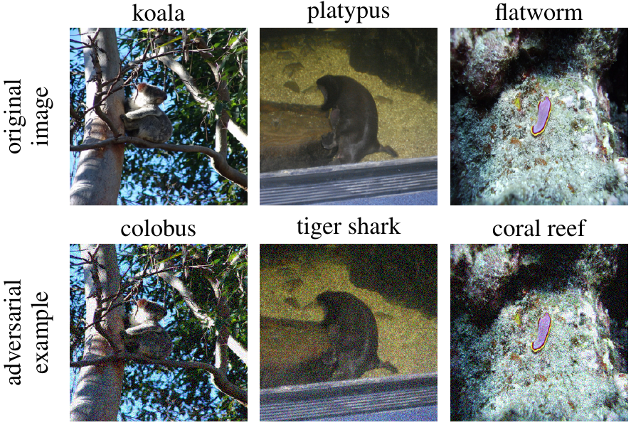
Figure 1: The legitimate images and their adversarial examples generated by ZO-NGD.

Ablation study

In this ablation study, we perform sensitivity analysis on the proposed ZO-NGD method based variations in model architectures and different parameter settings. Below we summarize the conclusion and findings from this ablation study and report their details in the appendix. (1) Tested on VGG16 and ResNet and varying the parameters $\mu$ and $\epsilon$ in ZO-NGD, the results demonstrate the consistent superior performance of ZO-NGD by leveraging the second-order optimization. (2) We inspect the approximation techniques used in ZO-NGD including damping and outer product method. The results show that there is a wide range of proper $\gamma$ values such that damping can work effectively to reduce the loss, and the outer product is a reasonable approximation based on the empirical evidence. We also note that the ASR of ZOO is higher than ZO-NGD. We provide a discussion about the ASR v.s. query number in the appendix.

Query Number Distribution

Figure 2 shows the cumulative distribution (CDF) of the query number for 1000 images on three datasets, validating ZO-NGD’s query efficiency.

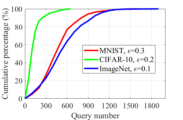
Figure 2: CDF of query number on three datasets using ZO-NGD.

Transferability

The transferability of adversarial examples is an interesting and valuable metric to measure the performance. To show the transferability, we use 500 targeted adversarial examples generated by ZO-NGD on ImageNet with $\epsilon=0.1$ on Inception to attack ResNet and VGG16 model. It achieves 94.4% and 95.6% ASR, respectively, demonstrating high transferability of our method. Our transferred ASR is also higher than NES-PGD (92.1% and 92.9% ASR).

Conclusion

In this paper, we propose a novel ZO-NGD to achieve high query-efficiency in black-box adversarial attacks. It incorporates the ZO random gradient estimation and the second-order FIM for NGD. The performance evaluation on three image classification datasets demonstrate the effectiveness of the proposed method in terms of fast convergence and improved query efficiency over state-of-the-art methods.

Disclaimer

This report was prepared as an account of work sponsored by an agency of the United States Government. Neither the United States Government nor any agency thereof, nor any of their employees, makes any warranty, express or implied, or assumes any legal liability or responsibility for the accuracy, completeness, or usefulness of any information, apparatus, product, or process disclosed, or represents that its use would not infringe privately owned rights. Reference herein to any specific commercial product, process or service by trade name, trademark, manufacturer, or otherwise does not necessarily constitute or imply its endorsement, recommendation, or favoring by the United States Government or any agency thereof. The views and opinions of authors expressed herein do not necessarily state or reflect those of the United States Government or any agency thereof.

Appendix A Appendix

Appendix B Geometric Interpretation

We provide a geometric interpretation for the natural gradient in this section. The negative gradient $-\nabla f(\bm{\delta})$ can be interpreted as the steepest descent direction in the sense that it yields the most reduction in $f$ per unit of change of $\bm{\delta}$, where the change is measured by the standard Euclidean norm $\left\|\cdot\right\|$ (?), as shown below,

$$\frac{{-\nabla f(\bm{\delta})}}{{\left\|{\nabla f(\bm{\delta})}\right\|}}=\mathop{\lim}\limits_{\epsilon\to 0}\frac{1}{\epsilon}\arg\mathop{\min}\limits_{\left\|\alpha\right\|\leq\epsilon}f(\bm{\delta}+\bm{\alpha}).$$ (24)

By following the $-\nabla f(\bm{\delta})$ direction, we can obtain the change of $\bm{\delta}$ within a certain $\epsilon$-neighbourhood to minimize the loss function.

As the loss function is related to the likelihood, we can explore the steepest direction to minimize the loss in the space of all possible likelihoods (i.e. distribution space). KL divergence (?) is a popular measure of the distance between two distributions. For two distributions $p\left(t|\bm{\delta}\right)$ and $p\left(t|\bm{\delta}^{\prime}\right)$, their KL divergence is defined as

$$\text{KL}\left[p\left(t|\bm{\delta}\right)||p\left(t|\bm{\delta}^{\prime}\right)\right]=\int{p\left(t|\bm{\delta}\right)\log\frac{p\left(t|\bm{\delta}\right)}{p\left(t|\bm{\delta}^{\prime}\right)}}dt.$$ (25)

Lemma 3

The FIM $\bm{F}$ is the Hessian of KL divergence between two distributions $p(t|\bm{\delta})$ and $p(t|\bm{\delta}+\bm{\alpha})$, with respect to $\bm{\alpha}$, evaluated at $\bm{\alpha}=\bm{0}$.

The proof is shown in the appendix. By Lemma 3, the FIM can be regarded as the curvature in the distribution space.

Lemma 4

The second order Taylor expansion of the KL divergence can be expressed as

$${\rm{KL}}\left[{p(t|{\bm{\delta}})||p(t|{\bm{\delta}}+{\bm{\alpha}})}\right]\approx\frac{1}{2}{{\bm{\alpha}}^{\rm{T}}}{\bf{F\bm{\alpha}}}.$$ (26)

We provide a proof in the appendix.

Next we explore the direction to minimize the loss function in the distribution space where the distance is measured by the KL divergence. Although in general, the KL divergence is not symmetric, it is (approximately) symmetric in a local neighborhood. The problem can be formulated as

$${{\bm{\alpha}}^{*}}=\mathop{\arg\min}\limits_{{\rm{KL}}\left[{p(t|{\bm{\delta}})||p(t|{\bm{\delta}}+{\bm{\alpha}})}\right]=m}f({\bm{\delta}}+{\bm{\alpha}}).$$ (27)

where $m$ is a certain constant. The purpose of fixing the KL divergence to a constant is to move along the distribution space with a constant speed, regardless of the curvature.

Thus, we can obtain Lemma 2 and show its proof in the appendix. In the parameter space, the negative gradient is the steepest descent direction to minimize the loss function. By contrast, in the distribution space, the steepest descent direction is the negative natural gradient. Thus, the direction in distribution space defined by the natural gradient will be invariant to the choice of parameterization (?), i.e., it will not be affected by how the model is parametrized, but only depends on the distribution induced by the parameters.

Appendix C Proof of Lemmas

Proof of Lemma 1

Proof of Lemma 1.

$$\mathop{\mathop{\mathbb{E}}\nolimits}\limits_{p(t,\bm{x}|\bm{\delta})}\left[{s({\bm{\delta}})}\right] =\mathop{\mathop{\mathbb{E}}\nolimits}\limits_{p(t,\bm{x}|\bm{\delta})}\left[{\nabla\log p(t,\bm{x}|\bm{\delta})}\right]$$

$$=\int{\nabla\log p(t,\bm{x}|\bm{\delta})}p(t,\bm{x}|\bm{\delta})dt\ d{\bm{x}}$$

$$=\int{\frac{{\nabla p(t,\bm{x}|\bm{\delta})}}{{p(t,\bm{x}|\bm{\delta})}}}p(t,\bm{x}|\bm{\delta})dt\ d{\bm{x}}$$

$$=\nabla\int p(t,\bm{x}|\bm{\delta})dt\ d{\bm{x}}$$

$$=0$$

Proof of Lemma 3

Proof of Lemma 3. The gradients of the KL divergence can be expressed as

$${\nabla_{\bf{\alpha}}}{\rm{KL}}\left[{p(t|{\bf{\delta}})||p(t|{\bf{\delta}}+{\bf{\alpha}})}\right] ={\nabla_{\bf{\alpha}}}\int{p(t|{\bf{\delta}})\log\frac{{p(t|{\bf{\delta}})}}{{p(t|{\bf{\delta}}+{\bf{\alpha}})}}}dt$$

$$={\nabla_{\bf{\alpha}}}\int{p(t|{\bf{\delta}})\log p(t|{\bf{\delta}})}dt$$

$$\ \ \ \ -{\nabla_{\bf{\alpha}}}\int{p(t|{\bf{\delta}})\log p(t|{\bf{\delta}}+{\bf{\alpha}})}dt$$

$$=-{\nabla_{\bf{\alpha}}}\int{p(t|{\bf{\delta}})\log p(t|{\bf{\delta}}+{\bf{\alpha}})}dt$$

$$=-\int{p(t|{\bf{\delta}}){\nabla_{\bf{\alpha}}}\log p(t|{\bf{\delta}}+{\bf{\alpha}})}dt$$ (28)

$$\nabla_{\bf{\alpha}}^{2}{\rm{KL}}\left[{p(t|{\bf{\delta}})||p(t|{\bf{\delta}}+{\bf{\alpha}})}\right]=-\int{p(t|{\bf{\delta}})\nabla_{\bf{\alpha}}^{2}\log p(t|{\bf{\delta}}+{\bf{\alpha}})}dt$$ (29)

The Hessian of the KL divergence is defined by

$${{\bf{H}}_{{\rm{KL}}\left[{p(t|{\bf{\delta}})||p(t|{\bf{\delta}}+{\bf{\alpha}})}\right]}} =-\int{p(t|{\bf{\delta}})\nabla_{\bf{\alpha}}^{2}\log p(t|{\bf{\delta}}+{\bf{\alpha}}){|_{{\bf{\alpha}}={\bf{0}}}}}dt$$

$$=-\int{p(t|{\bf{\delta}}){{\bf{H}}_{\log p(t|{\bf{\delta}})}}}dt$$

$$=-\mathop{E}\limits_{p(t|{\bf{\delta}})}\left[{{{\bf{H}}_{\log p(t|{\bf{\delta}})}}}\right]$$

$$={\bf{F}}$$ (30)

Proof of Lemma 4

Proof of Lemma 4.

$${\rm{KL}}\left[{p(t|{\bf{\delta}})||p(t|{\bf{\delta}}+{\bf{\alpha}})}\right] \approx{\rm{KL}}\left[{p(t|{\bf{\delta}})||p(t|{\bf{\delta}})}\right]$$

$$\ \ \ \ +{\left({\nabla_{\bf{\alpha}}{\rm{KL}}\left[{p(t|{\bf{\delta}})||p(t|{\bf{\delta}}+{\bf{\alpha}})}\right]{|_{{\bf{\alpha}}={\bf{0}}}}}\right)^{\rm{T}}}{\bf{\alpha}}$$

$$\ \ \ \ +\frac{1}{2}{{\bf{\alpha}}^{\rm{T}}}{\bf{F\alpha}}$$

$$={\rm{KL}}\left[{p(t|{\bf{\delta}})||p(t|{\bf{\delta}})}\right]$$

$$\ \ \ \ -\mathop{E}\limits_{p(t|{\bf{\delta}})}{\left[{\nabla_{\bf{\delta}}\log p(t|{\bf{\delta}})}\right]^{\rm{T}}}{\bf{\alpha}}$$

$$\ \ \ \ +\frac{1}{2}{{\bf{\alpha}}^{\rm{T}}}{\bf{F\alpha}}$$ (31)

Notice that the first term is zero as they are the same distributions. The second term is zero due to Lemma 1.

Proof of Lemma 2

Proof of Lemma 2. The Lagrangian function of the minimization can be formulated as

$$L({\bf{\alpha}}) =f({\bf{\delta}}+{\bf{\alpha}})+\phi\left({{\rm{KL}}\left[{p(t|{\bf{\delta}})||p(t|{\bf{\delta}}+{\bf{\alpha}})}\right]-c}\right)$$

$$\approx f({\bf{\delta}})+\nabla f{({\bf{\delta}})^{\rm{T}}}{\bf{\alpha}}+\frac{1}{2}\phi{{\bf{\alpha}}^{\rm{T}}}{\bf{F\alpha}}-\phi c$$ (32)

To solve this minimization, we set its derivative to zero:

$$\frac{\partial}{{\partial{\bf{\alpha}}}}\left({f({\bf{\delta}})+{\nabla_{\bf{\delta}}}f{{({\bf{\delta}})}^{\rm{T}}}{\bf{\alpha}}+\frac{1}{2}\varphi{{\bf{\alpha}}^{\rm{T}}}{\bf{F\alpha}}-\varphi c}\right)=0$$ (33)

$${\nabla_{\bf{\delta}}}f({\bf{\delta}})+\varphi{\bf{F\alpha}}=0$$ (34)

$${\bf{\alpha}}=-\frac{1}{\varphi}{{\bf{F}}^{-1}}{\nabla_{\bf{\delta}}}f({\bf{\delta}})$$ (35)

We can see that the negative natural gradient defines the steepest direction in the distribution space.

Appendix D Adversarial Examples

	3	6	8	7	5
MNIST
	deer	ship	truck	frog	cat
CIFAR

Figure A1: The legitimate images and their adversarial examples generated by ZO-NGD on MNIST and CIFAR-10. The misclassified class are shown on top of each image.

Appendix E Ablation study

Various Models

To check the performance of the proposed method on various model architecture, we performed experiments on three datasets using two new models (VGG16 & ResNet) and summarized the results in Table A1. The proposed ZO-NGD is more query-efficient than NES-PGD.

Table A1: Attack success rate (ASR) and query # for two new models.

	MNIST (VGG)		CIFAR10 (VGG)
	ASR	Query	ASR	Query
NES-PGD	99.2%	1082	98.3%	381
ZO-NGD	99.5%	548	98.2%	152
	ImageNet (VGG)		ImageNet (ResNet)
	ASR	Query	ASR	Query
NES-PGD	96.8%	1136	97.2%	1281
ZO-NGD	96.5%	594	98.1%	624

Parameter Analysis

The sensitivity analysis on the parameters $\mu$ and $\epsilon$ are demonstrated in Table A2. As observed form Table A2, the ZO-NGD performance is robust to different $\mu$ values (fixing $\epsilon=0.2$), and larger $\epsilon$ leads to fewer queries.

Table A2: Attack success rate (ASR) and query # for various hyper-parameters on ImageNet (Inception).

Value of $\mu$, while fixing $\epsilon=0.2$
1		0.1		0.01
ASR	Query	ASR	Query	ASR	Query
97.3%	626	97%	582	96.6%	596
Value of $\epsilon$, while fixing $\mu=0.1$
0.15		0.2		0.25
ASR	Query	ASR	Query	ASR	Query
96.1%	619	97%	583	98.2%	559

In second-order optimization, damping is a common technique to compensate for errors in the quadratic approximation. The parameter $\gamma$ plays a key role in damping. To show the influence of $\gamma$, we demonstrate the loss after 2 ADMM iterations for a wide range of $\gamma$ values with the same initialization in Figure A2(a). We observe that 0.01 or 0.001 is an appropriate choice for $\gamma$ to achieve higher query efficiency.

Drift of Outer Product

Although we adopt outer product (Equ. (12)) to approximate Equ. (9), we use the empirical evidence below to motivate why Equ. (12) dominates in Equ. (9) and the approximation is reasonable. For a well-trained model, the prediction probability of a correctly classified image usually dominates the probability distribution, that is, $p(t|\bm{x},\bm{\delta})$ is usually much larger than other probabilities if $t$ is correct and $\bm{\delta}$ is small. We plot the average prediction probability distribution of 1000 correctly classified images on CIFAR-10 and ImageNet for their top-10 labels in Figure A2(b). As observed from Figure A2(b), the correct label usually dominates in the probability distribution, leading to reasonable approximation loss from Equ. (9) to Equ. (12).

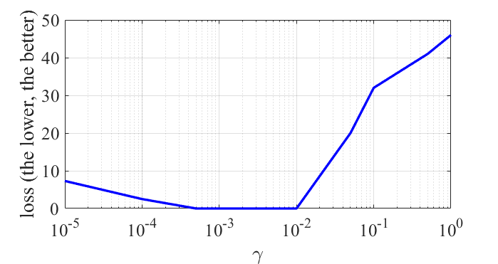
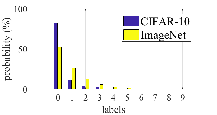
(a) Influence of $\gamma$ on MNIST	(b) probability distribution

Figure A2: Influence of $\gamma$ and prediction probability distribution. Prediction probability distribution on CIFAR-10/ImageNet.

References

- [Alzantot, Balaji, and Srivastava 2018] Alzantot, M.; Balaji, B.; and Srivastava, M. B. 2018. Did you hear that? adversarial examples against automatic speech recognition. CoRR abs/1801.00554.
- [Amari and Nagaoka 2007] Amari, S.-i., and Nagaoka, H. 2007. Methods of information geometry, volume 191. American Mathematical Soc.
- [Amari 1998] Amari, S.-I. 1998. Natural gradient works efficiently in learning. Neural Comput. 10(2):251–276.
- [Biggio, Fumera, and Roli 2014] Biggio, B.; Fumera, G.; and Roli, F. 2014. Security evaluation of pattern classifiers under attack. IEEE TKDE 26(4):984–996.
- [Brendel, Rauber, and Bethge 2017] Brendel, W.; Rauber, J.; and Bethge, M. 2017. Decision-based adversarial attacks: Reliable attacks against black-box machine learning models. arXiv preprint arXiv:1712.04248.
- [Bulò, Biggio, and et. al. 2017] Bulò, S. R.; Biggio, B.; and et. al. 2017. Randomized prediction games for adversarial machine learning. IEEE Transactions on Neural Networks and Learning Systems 28(11):2466–2478.
- [Carlini and Wagner 2017] Carlini, N., and Wagner, D. 2017. Towards evaluating the robustness of neural networks. In Security and Privacy (SP), 2017 IEEE Symposium on, 39–57. IEEE.
- [Chen et al. 2017a] Chen, P.-Y.; Sharma, Y.; Zhang, H.; Yi, J.; and Hsieh, C.-J. 2017a. Ead: elastic-net attacks to deep neural networks via adversarial examples. arXiv preprint arXiv:1709.04114.
- [Chen et al. 2017b] Chen, P.-Y.; Zhang, H.; Sharma, Y.; Yi, J.; and Hsieh, C.-J. 2017b. Zoo: Zeroth order optimization based black-box attacks to deep neural networks without training substitute models. In Proceedings of the 10th ACM Workshop on Artificial Intelligence and Security, 15–26. ACM.
- [Cox and Hinkley 1979] Cox, D. R., and Hinkley, D. V. 1979. Theoretical statistics. Chapman and Hall/CRC.
- [Demontis, Melis, and et. al. 2018] Demontis, A.; Melis, M.; and et. al. 2018. Yes, machine learning can be more secure! a case study on android malware detection. IEEE TDSC 1–1.
- [Deng et al. 2009] Deng, J.; Dong, W.; Socher, R.; Li, L.-J.; Li, K.; and Fei-Fei, L. 2009. Imagenet: A large-scale hierarchical image database. In Computer Vision and Pattern Recognition, 2009. CVPR 2009. IEEE Conference on, 248–255. IEEE.
- [Duchi et al. 2015] Duchi, J. C.; Jordan, M. I.; Wainwright, M. J.; and Wibisono, A. 2015. Optimal rates for zero-order convex optimization: The power of two function evaluations. IEEE Transactions on Information Theory 61(5):2788–2806.
- [Goodfellow, Shlens, and Szegedy 2015] Goodfellow, I.; Shlens, J.; and Szegedy, C. 2015. Explaining and harnessing adversarial examples. 2015 ICLR arXiv preprint arXiv:1412.6572.
- [Grosse and Martens 2016] Grosse, R. B., and Martens, J. 2016. A kronecker-factored approximate fisher matrix for convolution layers. In ICML, volume 1, 2.
- [Grosse and Salakhudinov 2015] Grosse, R., and Salakhudinov, R. 2015. Scaling up natural gradient by sparsely factorizing the inverse fisher matrix. In Bach, F., and Blei, D., eds., Proceedings of the 32nd International Conference on Machine Learning, volume 37 of Proceedings of Machine Learning Research, 2304–2313. Lille, France: PMLR.
- [Ilyas et al. 2018] Ilyas, A.; Engstrom, L.; Athalye, A.; and Lin, J. 2018. Black-box adversarial attacks with limited queries and information. In Proceedings of the 35th International Conference on Machine Learning, ICML 2018.
- [Ilyas, Engstrom, and Madry 2018] Ilyas, A.; Engstrom, L.; and Madry, A. 2018. Prior convictions: Black-box adversarial attacks with bandits and priors. ICLR 2019.
- [Karakida, Akaho, and Amari 2018] Karakida, R.; Akaho, S.; and Amari, S.-i. 2018. Universal statistics of fisher information in deep neural networks: Mean field approach. arXiv preprint arXiv:1806.01316.
- [Krizhevsky and Hinton 2009] Krizhevsky, A., and Hinton, G. 2009. Learning multiple layers of features from tiny images. Master’s thesis, Department of Computer Science, University of Toronto.
- [Kullback and Leibler 1951] Kullback, S., and Leibler, R. A. 1951. On information and sufficiency. Ann. Math. Statist. 22(1):79–86.
- [LeCun, Bengio, and Hinton 2015] LeCun, Y.; Bengio, Y.; and Hinton, G. 2015. Deep learning. 521:436–44.
- [Lecun et al. 1998] Lecun, Y.; Bottou, L.; Bengio, Y.; and Haffner, P. 1998. Gradient-based learning applied to document recognition. Proceedings of the IEEE 86(11):2278–2324.
- [Li et al. 2019] Li, Z.; Ding, C.; Wang, S.; Wen, W.; Zhuo, Y.; Liu, C.; Qiu, Q.; Xu, W.; Lin, X.; Qian, X.; and Wang, Y. 2019. E-rnn: Design optimization for efficient recurrent neural networks in fpgas. In 2019 IEEE International Symposium on High Performance Computer Architecture (HPCA), 69–80.
- [Lin, Hong, and et. al. 2017] Lin, Y.-C.; Hong, Z.-W.; and et. al. 2017. Tactics of adversarial attack on deep reinforcement learning agents. In Proceedings of the 26th International Joint Conference on Artificial Intelligence, 3756–3762. AAAI Press.
- [Liu et al. 2019] Liu, S.; Chen, P.-Y.; Chen, X.; and Hong, M. 2019. SignSGD via zeroth-order oracle. International Conference on Learning Representations.
- [Madry et al. 2017] Madry, A.; Makelov, A.; Schmidt, L.; Tsipras, D.; and Vladu, A. 2017. Towards deep learning models resistant to adversarial attacks. arXiv preprint arXiv:1706.06083.
- [Martens and Grosse 2015] Martens, J., and Grosse, R. 2015. Optimizing neural networks with kronecker-factored approximate curvature. In International conference on machine learning, 2408–2417.
- [Martens 2014] Martens, J. 2014. New perspectives on the natural gradient method. CoRR abs/1412.1193.
- [Martens 2016] Martens, J. 2016. Second-order optimization for neural networks. University of Toronto (Canada).
- [Nesterov and Spokoiny 2017] Nesterov, Y., and Spokoiny, V. 2017. Random gradient-free minimization of convex functions. Foundations of Computational Mathematics 17(2):527–566.
- [Ollivier 2015] Ollivier, Y. 2015. Riemannian metrics for neural networks i: feedforward networks. Information and Inference: A Journal of the IMA 4(2):108–153.
- [Osawa et al. 2018] Osawa, K.; Tsuji, Y.; Ueno, Y.; Naruse, A.; Yokota, R.; and Matsuoka, S. 2018. Second-order optimization method for large mini-batch: Training resnet-50 on imagenet in 35 epochs. CVPR 2019.
- [Papernot, McDaniel, and Goodfellow 2016] Papernot, N.; McDaniel, P. D.; and Goodfellow, I. J. 2016. Transferability in machine learning: from phenomena to black-box attacks using adversarial samples. CoRR abs/1605.07277.
- [Pascanu and Bengio 2013a] Pascanu, R., and Bengio, Y. 2013a. Natural gradient revisited. CoRR abs/1301.3584.
- [Pascanu and Bengio 2013b] Pascanu, R., and Bengio, Y. 2013b. Revisiting natural gradient for deep networks. arXiv preprint arXiv:1301.3584.
- [Szegedy et al. 2016] Szegedy, C.; Vanhoucke, V.; Ioffe, S.; Shlens, J.; and Wojna, Z. 2016. Rethinking the inception architecture for computer vision. CVPR 2016 2818–2826.
- [Tu et al. 2018] Tu, C.-C.; Ting, P.; Chen, P.-Y.; Liu, S.; Zhang, H.; Yi, J.; Hsieh, C.-J.; and Cheng, S.-M. 2018. Autozoom: Autoencoder-based zeroth order optimization method for attacking black-box neural networks. arXiv preprint arXiv:1805.11770.
- [Wang et al. 2018a] Wang, S.; Wang, X.; Ye, S.; Zhao, P.; and Lin, X. 2018a. Defending dnn adversarial attacks with pruning and logits augmentation. In 2018 IEEE Global Conference on Signal and Information Processing (GlobalSIP), 1144–1148.
- [Wang et al. 2018b] Wang, S.; Wang, X.; Zhao, P.; Wen, W.; Kaeli, D.; Chin, P.; and Lin, X. 2018b. Defensive dropout for hardening deep neural networks under adversarial attacks. In ICCAD ’18.
- [Wang et al. 2018c] Wang, Y.; Du, S.; Balakrishnan, S.; and Singh, A. 2018c. Stochastic zeroth-order optimization in high dimensions. In AISTATS 2018, volume 84 of Proceedings of Machine Learning Research. PMLR.
- [Wang et al. 2019] Wang, X.; Wang, S.; Chen, P.-Y.; Wang, Y.; Kulis, B.; Lin, X.; and Chin, S. 2019. Protecting neural networks with hierarchical random switching: Towards better robustness-accuracy trade-off for stochastic defenses. In IJCAI 2019.
- [Xie, Wang, and et. al. 2018] Xie, C.; Wang, J.; and et. al. 2018. Adversarial examples for semantic segmentation and object detection. In ICCV 2017, 1378–1387.
- [Xu et al. 2018] Xu, K.; Liu, S.; Zhao, P.; Chen, P.-Y.; Zhang, H.; Erdogmus, D.; Wang, Y.; and Lin, X. 2018. Structured Adversarial Attack: Towards General Implementation and Better Interpretability. ArXiv e-prints.
- [Xu et al. 2019] Xu, K.; Chen, H.; Liu, S.; Chen, P.-Y.; Weng, T.-W.; Hong, M.; and Lin, X. 2019. Topology attack and defense for graph neural networks: An optimization perspective. arXiv preprint arXiv:1906.04214.
- [Ye et al. 2018] Ye, H.; Huang, Z.; Fang, C.; Li, C. J.; and Zhang, T. 2018. Hessian-aware zeroth-order optimization for black-box adversarial attack. CoRR abs/1812.11377.
- [Zhang, Weng, and et. al. 2018] Zhang, H.; Weng, T.-W.; and et. al. 2018. Efficient Neural Network Robustness Certification with General Activation Functions. In NIPS 2018.
- [Zhao et al. 2017] Zhao, A.; Fu, K.; Wang, S.; Zuo, J.; Zhang, Y.; Hu, Y.; and Wang, H. 2017. Aircraft recognition based on landmark detection in remote sensing images. IEEE Geoscience and Remote Sensing Letters 14(8):1413–1417.
- [Zhao et al. 2018] Zhao, P.; Liu, S.; Wang, Y.; and Lin, X. 2018. An admm-based universal framework for adversarial attacks on deep neural networks. In ACM Multimedia 2018.
- [Zhao et al. 2019a] Zhao, P.; Liu, S.; Chen, P.-Y.; Hoang, N.; Xu, K.; Kailkhura, B.; and Lin, X. 2019a. On the design of black-box adversarial examples by leveraging gradient-free optimization and operator splitting method. In ICCV 2019.
- [Zhao et al. 2019b] Zhao, P.; Wang, S.; Gongye, C.; Wang, Y.; Fei, Y.; and Lin, X. 2019b. Fault sneaking attack: A stealthy framework for misleading deep neural networks. In DAC 2019.
- [Zhao et al. 2019c] Zhao, P.; Xu, K.; Liu, S.; Wang, Y.; and Lin, X. 2019c. Admm attack: An enhanced adversarial attack for deep neural networks with undetectable distortions. In ASPDAC 2019.