Observational nonidentifiability, generalized likelihood and free energy

Abstract

We study the parameter estimation problem in mixture models with observational nonidentifiability: the full model (also containing hidden variables) is identifiable, but the marginal (observed) model is not. Hence global maxima of the marginal likelihood are (infinitely) degenerate and predictions of the marginal likelihood are not unique. We show how to generalize the marginal likelihood by introducing an effective temperature, and making it similar to the free energy. This generalization resolves the observational nonidentifiability, since its maximization leads to unique results that are better than a random selection of one degenerate maximum of the marginal likelihood or the averaging over many such maxima. The generalized likelihood inherits many features from the usual likelihood, e.g. it holds the conditionality principle, and its local maximum can be searched for via suitably modified expectation-maximization method. The maximization of the generalized likelihood relates to entropy optimization.

I Introduction

Unknown parameters of mixture models are frequently estimated via the Maximum Marginal Likelihood (MML) method that employs the marginal probability of the observed data pawitan ; cox ; jelinek_review ; rabiner_review ; ephraim_review . A local maximization of the marginal likelihood can be carried out via one of computationally feasible algorithms, e.g. the Expectation-Maximization (EM) method jelinek_review ; rabiner_review ; ephraim_review .

There is however a range of problems, where MML does not apply due to observational nonidentifiability: the full model (including hidden variables) is identifiable, but the observed (marginal) model is not. Hence the maxima of the marginal likelihood are (generally infinitely) degenerate, and the outcome of MML does depend on the initial point of the maximization. Resolving the nonidentifiability in such situations is not hopeless, precisely because the full model is identifiable. However, the standard likelihood maximization cannot be employed, since there are hidden (not observed) variables. We emphasize that some information about unknown parameters is always lost after marginalization cox . The observational nonidentifiability is an extreme case of this.

Nonidentifiability in mixture models is studied in teicher ; rothenberg ; ito ; watanabe ; hsiao ; ran_hu ; welcher ; manski ; allman ; gu ; see hsiao ; ran_hu ; welcher for reviews. In such models even an infinitely large number of observed data samples cannot guarantee the perfect recovery of parameters (i.e. the convergence to true parameter values), because maxima of the likelihood are infinitely degenerate rothenberg . There is an attitude towards nonidentifiable models that they are in a certain sense rare, and do not have a big practical importance. This is incorrect: almost any model becomes nonidentifiable if the number of unknown parameters is sufficiently large, i.e. if the model is sufficiently realistic watanabe ; hsiao . Moreover, nonidentifiability can be present effectively due to unresponsiveness of a many-parameter likelihood along sufficiently many directions sethna1 ; sethna2 ; see sethna3 for a review. The simplest scenario of this is realized via small eigenvalues of the likelihood Hessian. For practical purposes such an effective nonidentifiability—which is generically found in systems biology and chemistry sethna1 ; sethna2 ; sethna3 —is indistinguishable from the true one.

Aiming to solve the problem of observational nonidentifiability, we extend the marginal likelihood via a one-parameter generalized function ${L}_{\beta}$, which is constructed by analogy to the free energy in statistical physics. The positive parameter $\beta$ is an analogue of the inverse temperature from statistical physics, and the marginal likelihood is recovered for $\beta=1$. We show that ${L}_{\beta}$ inherits pertinent features of ${L}_{1}$; e.g. it holds the conditionality principle, concavity (for $\beta\leq 1$) and the possibility to search for its local maximum via suitably generalized expectation-maximization method. Its maximization resolves the degeneracy of $L_{1}$. It does have relations with the maximum entropy method (for $\beta<1$) and with entropy minimization (for $\beta>1$). For several models we found an optimal value of $\beta$ in ${L}_{\beta}$, which appears to be close to 1, but strictly smaller than $1$. We also show numerically that maximizing ${L}_{\beta\lesssim 1}$ leads to better results than (i) a random selection of one of many results provided by maximizing the usual likelihood ${L}_{1}$; (ii) averaging over many such random selections; see section V. Both (i) and (ii) would be among standard reactions of practitioners to (effective) nonidentifiability.

For $\beta\to\infty$ we get another known quantity: ${L}_{\infty}$ coincides with the h-likelihood pawitan ; jelinek_review ; rabiner_review ; ephraim_review , i.e. the full likelihood (including both observed and hidden variables), where the value of hidden variables is replaced by their maximum aposteriori (MAP) estimates from the observed data nelder ; bjorn ; scand . The h-likelihood is employed in Hidden Markov Models (HMM), where efficient methods of maximizing ${L}_{\infty}$ are known as Viterbi Training (VT) or k-means segmentation jelinek_review ; rabiner_review ; ephraim_review ; rabiner ; merhav . When the h-likelihood ${L}_{\infty}$ is applied to an observationally nonidentifiable situation, its results converge to boundary values of the parameters (e.g. zero or one for unknown probabilities), as was demonstrated by analyzing an exactly solvable HMM model nips . Such results are inferior to random selection (see (i) and (ii) above), if there is no prior information that the model is indeed sparse in this sense; cf. section VI. This feature is one reason why the h-likelihood maximization leads to obvious failures even in simple models nelder ; meng . In particular, it cannot apply generally for solving observational nonidentifiability.

$L_{\beta}$ also relates to a recent trend in the Bayesian statistics, where the model is raised to a certain positive power, akin to $\beta\not=1$ in $L_{\beta}$ bissiri ; holmes ; hagan ; friel ; miller . In this way people deal with misspecified models bissiri ; holmes ; miller , facilitate the computation of Bayesian factors for model selection friel , regularize them hagan etc; see miller for a recent review. The raising into a power emerges from the decision theory (as applied to misspecified models) bissiri and present a general method for making Bayesian models more robust. Among the actively researched issues here is the selection of the power parameter holmes .

This paper is written in the style of the book by Cox and Hinkley cox : it is example-based and informal, not the least because it employs ideas of statistical physics. It is organized as follows. Section II.1 recalls the definition of the observational nonidentifiability we set to study. Section II.2 defines the generalized likelihood $L_{\beta}$, and discusses its features inherited from the usual likelihood $L_{1}$. Sections II.3 and II.4 study the simplest nonidentifiable examples that illustrates features of $L_{\beta}$. Section III defines the main model we shall focus on. It amounts to a finite mixture with unknown probabilities. Section IV studies for this model the generalized likelihood $L_{\beta<1}$. Numerical comparison with the random selection methods is discussed in section V. Section IV studies the maximization of $L_{\beta>1}$ and shows in which sense this is related to entropy minimization. We summarize in the last section.

II Free energy as generalized likelihood

II.1 Defining observational nonidentifiability

We are given two random variables $X$ and $Y$ with values $x=(x_{1},...,x_{n})$ and $y=(y_{1},...,y_{m})$, respectively. We assume that $X$ is hidden, while $Y$ observed variable, i. e. we assume a mixture model. The joint probabilities of $XY$

$$p_{\theta}(x,y),$$ (1)

generally depend on unknown parameters $\theta$. Let we are given the observation data

$$\{\,y^{[k]}\,\}_{k=1}^{N},$$ (2)

where $y^{[k]}$ are values of $Y$ generated independently from each other. Then $\theta$ can be estimated via the (marginal, logarithmic) likelihood

$$L(\theta)=\frac{1}{N}\sum_{k=1}^{N}\ln\left[p_{\theta}(y^{[k]})\right]=\sum_{y}p(y)\ln\left[\sum_{x}p_{\theta}(x,y)\right],$$ (3)

where $p(y_{1}),...,p(y_{m})$ are the frequencies of $Y$ obtained from the data (2). If (for a fixed $m$) the observation data (2) is large, $N\gg 1$, $p(y)$ converge to true probabilities of $Y$.

Within the maximum likelihood method, the unknown $\theta$ can be determined from ${\rm argmax}_{\theta}[\,L(\theta)]$. Since $X$ is a hidden, we can easily run into the nonidenitifiability problem, where (at least two) different values of $\theta$ lead to the same probability for all values of $Y$ teicher ; rothenberg ; ito ; hsiao :

$$p_{\theta}(y_{l})=p_{\theta^{\prime}}(y_{l}),\quad l=1,...,m,\quad\theta\not=\theta^{\prime}.$$ (4)

Eqs. (4) imply that maxima of $L(\theta)$ are degenerate; see below for examples. In addition to (4), we shall require that the full model is still identifiable, i.e. imposing equal joint probabilities for for all $(x,y)$ does lead to $\theta=\theta^{\prime}$ for all $(\theta,\theta^{\prime})$:

$$p_{\theta}(x_{k},y_{l})=p_{\theta^{\prime}}(x_{k},y_{l}),\quad k=1,...,n,~{}l=1,...,m,\quad\Longrightarrow\quad\theta=\theta^{\prime}.$$ (5)

We shall propose a solution to this type of nonidentifiability. Below we shall focus the most acute situation, where the marginal probability in (4) does not depend on $\theta$ and the sample length in (2) is very large: $N\gg 1$. Note that other (weaker) forms of nonidentifiability are possible and well-documented in literature: the weakest form of nonidentifiability is when it is restricted to a measure-zero subset of the parameter domain (generic identifiability) allman . A stronger form is that of partial nonidentifiability, where some information on $\theta$ (e.g. certain bounds on $\theta$) can still be recovered from observations; see gu for a recent discussion.

II.2 Generalized likelihood: definition and features

II.2.1 Definition

Instead of (3) we set to maximize over $\theta$ its generalization, viz. the negative free-energy

$$L_{\beta}(\theta)=\frac{1}{\beta}\sum_{y}p(y)\ln\left[\sum_{x}p_{\theta}^{\beta}(x,y)\right],$$ (6)

where $\beta>0$ is a parameter. An obvious feature of (6) is that for $\beta=1$ we return from (6) to the (marginal) likelihood function $L(\theta)$ in (3). Hence if we apply the maximization of (6) with $\beta\approx 1$ to the identifiable model, we expect to get results that are close to those found via maximization of $L(\theta)$. The meaning of $\beta\not=1$ in (6) is that it sums over all values of $x$, but does not reduce the outcome to the usual (marginal) likelihood.

Below we discuss several features that $L_{\beta}(\theta)$ inherits from the usual likelihood $L_{1}(\theta)=L(\theta)$. These features motivate introducing $L_{\beta}(\theta)$ as a generalization of $L_{1}(\theta)$. The first such feature is apparent from the fact that $L_{\beta}(\theta)$ in (6) is to be maximized over unknown parameter $\theta$ pawitan . If we reparametrize $L_{\beta}$ via a bijective (one-to-one) function $\psi(\theta)$—i.e. if the full information on $\theta$ is retained in $\psi$—then the maximization outcomes

$$\hat{\psi}={\rm argmax}_{\psi}[L_{\beta}(\psi)]\quad{\rm and}\quad\hat{\theta}={\rm argmax}_{\theta}[L_{\beta}(\theta)],$$ (7)

are related via the same function: $\hat{\psi}=\psi(\hat{\theta})$.

II.2.2 Relations of (6) to nonequilibrium free energy

Relations between statistical physics and probabilistic inference frequently proceed via the Gibbs distribution, where the minus logarithm of probability to be inferred is interpreted as the physical energy (both these quantities are additive for independent events), while the physical temperature is taken to be $1$; see mezard for a textbook presentation of this analogy and lamont for a recent review. The main point of making this analogy is that powerful approximate methods of statistical physics can be applied to inference mezard ; lamont .

In the context of mixture models we can carry out the above analogy one step further. This analogy is now structural, i.e. it relates to the form of (6), and not to applicability of any approximate method. We relate $-\ln\hat{p}(x,y)$ with the energy of a physical system, where $X$ and $Y$ are respectively fast (hidden) and slow (observed) variables. Here fast and slow connect with (resp.) hidden and observed, which agrees with the set-up of statistical physics, where only a part of variables is observed free . Then (6) connects to the negative nonequilibrium free energy with inverse temperature $\beta$ free . Here nonequilibrium means that only one variable (i.e. $X$) is thermalized (i.e. its conditional probability is Gibbsian), while the free energy has several physical meanings free ; e.g. it is a generating function for calculating various averages and also the (physical) work done under a slow change of suitable externally-driven parameters free . The maximization of (6) naturally relates to the physical tendency of decreasing free energy (one formulation of the second law of thermodynamics) free .

Though formal, this correspondence with statistical physics will be instrumental in interpreting $L_{\beta}$. E.g. we shall see that the maximizer of $L_{\beta<1}$ is unique (in contrast to maximizers of $L_{\beta\geq 1}$), and this fact can be related to sufficiently high temperatures that simplify the free energy landscape.

II.2.3 Relations with h-likelihood

For $\beta\to\infty$ we revert from (6) to

$$L_{\infty}(\theta)=\sum_{y}p(y)\ln\left[{\rm max}_{x}\,p_{\theta}(x,y)\right],$$ (8)

where ${\rm argmax}_{x}\hat{p}_{\theta}(x,y)$ is the MAP (maximum aposteriori) estimate of $x$ given the data $y$ ephraim_review ; rabiner ; nips . The meaning of (8) is obvious in the context of (5): once we cannot employ the maximum likelihood method to $p_{\theta}(x,y)$—since we do not know what to take for the hidden variable $x$—we first estimate $x$ from data (2) via the MAP method, and then proceed a la usual likelihood .

It is known that maximizing over unobserved variables has drawbacks pawitan ; nelder ; meng . People tried to improve on those drawbacks by looking instead of (8) at byrne

$$\frac{1}{U}\sum_{u=1}^{U}\sum_{y}p(y)\ln\left[p_{\theta}(x_{[u]}(y),y)\right],$$ (9)

where $U=2,3$, $x_{[1]}(y)$ maximizes $p(x,y)$ over $x$, $x_{[2]}(y)$ is the next to the maximal value of $p(x,y)$ etc. In contrast to (8), Eq. (9) accounts for values of $x$ around the maximum of $p(x,y)$. Now $L_{\beta}(\theta)$ captures the same idea for a large but finite $\beta$.

II.2.4 Conditionality

It is known that the ordinary maximum-likelihood method has an appealing feature of conditionality, which is formulated in several related forms cox , and closely connects to other fundamental principles of statistics, e.g. to the likelihood principle cox ; berger ; evans . We now find out to which extent the conditionality principle is inherited by the generalized likelihood $L_{\beta}$ defined in (6).

First we note that $L_{\beta}$ holds the weak conditionality principle berger . To define this principle we should enlarge the original pair $(X,Y)$ of random variables to $(X,Y,J)$, where $J$ assumes (for simplicity) a finite set of values $j_{1},..,j_{\ell}$. Now $X$ and $Y$ are still (resp.) hidden and observed variables, while $J$ determines the choice of the experiment that does not depend on the unknown parameter $\theta$ berger ; evans . The choice is done before observing $Y$, i.e. before collecting the sample (2), and the (marginal) probability $p(j)$ does not depend on $\theta$. For this extended experiment the data amounts to sample (2) plus the indicator $j$ for the choice of the experiment. Then the analogue of (6) is defined as

$${L}_{\beta}(j,\theta)=\frac{1}{\beta}\sum_{y}p(y)\ln\left[\sum_{x}p^{\beta}_{\theta}(x,y,j)\right]=\frac{1}{\beta}\sum_{y}p(y)\ln\left[\sum_{x}p^{\beta}_{\theta}(x,y|j)\right]+\ln p(j),$$ (10)

where $p_{\theta}(x,y,j)$ is the probability of $(X,Y,J)$. It is seen that the inference for the extended experiment produces the same result as the inference for the partial experiment, where the value of $J=j$ was fixed beforehands (i.e. the choice of $J=j$ was not a part of data):

$${\rm argmax}_{\theta}\left({L}_{\beta}(j,\theta)\right)={\rm argmax}_{\theta}\left(\frac{1}{\beta}\sum_{y}p(y)\ln\left[\sum_{x}p^{\beta}_{\theta}(x,y|j)\right]\right).$$ (11)

This is the weak conditionality principle that holds for the generalized likelihood $L_{\beta}(\theta)$.

However, a stronger form of the conditionality principle does not hold for $L_{\beta}(\theta)$, because this form mixes observable and hidden variables. Define a new random variable $G(X,Y)$ that depends on $X$ and $Y$ and assumes values $g_{1},...,g_{\ell}$ cox . Assume that the marginal probability $p(g)$ of $G$ does not depend on $\theta$, i.e. $G$ is an ancillary variable with respect to estimating $\theta$ fraser_review . Now (6) reads

$${L}_{\beta}(\theta)=\frac{1}{\beta}\sum_{y}p(y)\ln\left[\sum_{g\in{\cal G}(y)}p^{\beta}(g)\sum_{x:\,G(x,y)=g}p^{\beta}_{\theta}(x,y|g)\right],$$ (12)

where ${\cal G}(y)\subset(g_{1},...,g_{\ell})$ is the set of values assumed by $G(x,y)$, where $y$ is fixed, while $x$ goes over all its values $(x_{1},..,x_{n})$. One defines a new experiment, where it is a priori known that the value of $G(X,Y)$ is restricted to a specific value $g$ from $(g_{1},...,g_{\ell})$. The generalized likelihood for this experiment is

$${L}_{\beta}(\theta|G=g)=\frac{1}{\beta}\sum_{y}p(y)\ln\left[\sum_{x:\,G(x,y)=g}p^{\beta}_{\theta}(x,y|g)\right].$$ (13)

It is seen that for $\beta\not=1$ the maximization of (12) and (13) will generally produce different results, i.e. the stronger form of the conditionality principle does not hold for $L_{\beta}$.

II.2.5 Monotonicity and concavity

$L_{\beta}(\theta)$ is monotonically decreasing over $\beta$:

$$\frac{\partial L_{\beta}(\theta)}{\partial\beta}=\frac{1}{\beta^{2}}\sum_{y}p(y)\sum_{x}\zeta_{\theta}(x|y;\beta)\ln\zeta_{\theta}(x|y;\beta)\leq 0,$$ (14)

$$\zeta_{\theta}(x|y;\beta)\equiv\left.{p_{\theta}^{\beta}(x,y)}\right/{{\sum}_{\bar{x}}p_{\theta}^{\beta}(\bar{x},y)},$$ (15)

since $\frac{\partial L_{\beta}(\theta)}{\partial\beta}$ is a weighted sum of negative entropies.

Let $\theta\in\Omega$ is defined over a partially convex set $\Omega$, i.e. if $\theta_{1}\in\Omega$ and $\theta_{2}\in\Omega$, then for $0<\lambda<1$ there exists $\theta_{3}\in\Omega$ such that $p_{\theta_{3}}=\lambda p_{\theta_{1}}+(1-\lambda)p_{\theta_{2}}$; such a model is studied below in section III. Now for $\beta\leq 1$, $L_{\beta}$ from (6) is a concave function, since it is a linear combination of superposition of two strictly concave functions: $f(u)=u^{\beta}$ and $g(v)=\ln v$:

$$L_{\beta}(\lambda p_{\theta_{1}}+(1-\lambda)p_{\theta_{2}})>\lambda L_{\beta}(p_{\theta_{1}})+(1-\lambda)L_{\beta}(p_{\theta_{2}}),\qquad\beta\leq 1.$$ (16)

For $\beta>1$, we note that a superposition $g(f(u))$ of strictly convex $f(u)=u^{\beta}$ and monotonic $g(v)=\ln v$ is pseudo-convex pseudoconvex . Pseudo-convex functions do share many important features of convex functions, but generally $L_{\beta>1}$ is not pseudo-convex, since besides superposition of $f(u)=u^{\beta}$ and $g(v)=\ln v$, (6) involves summation over $y$, and the sum of two pseudo-convex functions is generally not pseudo-convex pseudoconvex . In section VI we shall show numerically that maximizers of $L_{\beta>1}$ relate to those of a generalized Schur-convex function; see Appendix D.

II.2.6 Relations with the maximum entropy method

The maximization of the generalized likelihood (6) will be now related with the maximum entropy method jaynes ; jaynes_2 ; skyrms ; enk ; cheeseman . Recall that the method addresses the problem of recovering unknown probabilities $\{q(z_{k})\}_{k=1}^{n}$ of a random variable $Z=(z_{1},...,z_{n})$ on the ground of certain contraints on $q$ and $Z$. The type and number of those constrains are not decided within the method itself jaynes_2 ; enk , though the method can give some recommendations for selecting relevant constraints; see Appendix C. Then $\{q(z_{k})\}_{k=1}^{n}$ are determined from the constrained maximization of the entropy $-\sum_{k=1}^{n}q(z_{k})\ln q(z_{k})$ jaynes ; jaynes_2 ; skyrms ; enk ; cheeseman . The intuitive rationale of the method is that it provides the most unbiased choice of probability compatible with constraints.

To find this relation, we expand (6) for a small $1-\beta$ (i.e. $\beta\simeq 1$)

$$L_{\beta}(\theta) = \sum_{y}p(y)\ln p_{\theta}(y)+\frac{1}{\beta}\sum_{y}p(y)\ln\left[\sum_{x}p_{\theta}(x|y)e^{(\beta-1)\ln p_{\theta}(x|y)}\right]$$ (17)

$$= \sum_{y}p(y)\ln p_{\theta}(y)+(1-\beta)\sum_{y}p(y)S_{y}(\theta)+(1-\beta)^{2}\sum_{y}p(y)S_{y}(\theta)$$ (18)

$$+ \frac{(1-\beta)^{2}}{2}\sum_{xy}p(y)p_{\theta}(x|y)\left(\,-S_{y}(\theta)+\ln p_{\theta}(x|y)\,\right)^{2}+{\cal O}\left((1-\beta)^{3}\right),$$ (19)

$$S_{y}(\theta) \equiv -\sum_{x}p_{\theta}(x|y)\ln p_{\theta}(x|y),$$ (20)

where $S_{y}(\theta)$ is the entropy of $X$ for a fixed observation $Y=y$ and fixed parameters $\theta$. When expanding $e^{(\beta-1)\ln p_{\theta}(x|y)}$ over ${(\beta-1)\ln p_{\theta}(x|y)}$ we need to assume that $p_{\theta}(x|y)>0$, but eventually a milder condition $p_{\theta}(x|y)\geq 0$ suffices because the terms in (18–20) stay finite for $p_{\theta}(x|y)\to 0$.

The zero-order term in $L_{\beta}(\theta)$ is naturally $L(\theta)=\sum_{y}p(y)\ln p_{\theta}(y)$; see (18). But, as we explained around (4), even when $N\gg 1$ in (16), the maximization of $L_{1}$ does not lead to a single result if the model is not identifiable. This degeneration will be (at least partially) lifted if the next-order term $(1-\beta)\sum_{y}p(y)S_{y}(\theta)$ in $L_{\beta}$ is taken into account; cf. (18). For $\beta<1$ this term will tend to lift the degeneracy by selecting those maxima which achieve the largest average entropy $\sum_{y}p(y)S_{y}(\theta)$. Hence for a small, but positive $1-\beta$, the results of maximazing $\sum_{y}p(y)\ln p_{\theta}(y)$ will (effectively) serve as constraints when maximizing $\sum_{y}p(y)S_{y}(\theta)$. This is the relation between maximizing $L_{\beta}$ (for a small, positive $1-\beta$) and entropy maximization .

Note that when $p(y)$ converges to the true probabilities of $Y$, i.e. when $N\gg 1$ in (16), and when $\theta$ is fixed to its true value, then $\sum_{y}p(y)S_{y}(\theta)$ is the conditional entropy of $X$ given $Y$ jaynes_2 . The appearance of the conditional entropy is reasonable given the fact that $Y$ is an observed variable.

Within the second-order term ${\cal O}\left((1-\beta)^{2}\right)$ the fluctuations of entropy enter into consideration: the degeneration will be lifted by (simultaneously) maximizing the entropy variance and maximizing the entropy; see (18, 19).

Likewise, for $\beta>1$ (but $\beta\simeq 1$) the term $(1-\beta)\sum_{y}p(y)S_{y}(\theta)$ in $L_{\beta}(\theta)$ predicts that among degenerate maxima of $L_{1}(\theta)$, those of the minimal entropy will be selected.

II.2.7 $Q$-function and generalized EM procedure

$L_{\beta}(\theta)$ in (6) admits a representation via a suitably generalized $Q$-function, i.e. its local maximum can be calculated via the (generalized) expectation-maximization (EM) algorithm. Let us define for two different values of $\theta$ and $\widetilde{\theta}$:

$$Q_{\beta}(\theta,\widetilde{\theta})=\sum_{y}p(y)\sum_{x}\zeta_{\theta}(x|y;\beta)\ln{p}_{\widetilde{\theta}}(x,y),$$ (21)

where $\zeta_{\theta}(x|y;\beta)$ defined by (15) is formally a conditional probability. For $\beta=1$ we revert from (21) to the average of the usual $Q$-function ephraim_review ; wu : $\sum_{x}p_{\theta}(x|y)\ln{p}_{\widetilde{\theta}}(x,y)$, which is the full log-likelihood $\ln{p}_{\widetilde{\theta}}(x,y)$ that is averaged over the hidden variable $X$ given the observed $Y=y$ and calculated at trial values $\theta$ and $\widetilde{\theta}$.

Now non-negativity of the relative entropy:

$$\frac{1}{\beta}\sum_{y}p(y)\sum_{x}\zeta_{\theta}(x|y;\beta)\ln\frac{\zeta_{\theta}(x|y;\beta)}{\zeta_{\widetilde{\theta}}(x|y;\beta)}\geq 0,$$ (22)

implies after using (15, 21) and re-arranging (22):

$$L_{\beta}(\widetilde{\theta})-L_{\beta}({\theta})\geq Q_{\beta}(\theta,\widetilde{\theta})-Q_{\beta}(\theta,{\theta}).$$ (23)

Hence if for a fixed $\theta$ we choose $\widetilde{\theta}$ such that $Q_{\beta}(\theta,\widetilde{\theta})>Q_{\beta}(\theta,{\theta})$, then this will increase $L_{\beta}(\widetilde{\theta})$ over $L_{\beta}({\theta})$. Eq. (23) shows the main idea of EM: defining

$$\theta_{k+1}={\rm argmax}_{\widetilde{\theta}}[\,Q_{\beta}(\theta_{k},\widetilde{\theta})\,],$$ (24)

and starting from trial value $\theta_{1}$, we increase $L_{\beta}({\theta})$ sequentially, $L_{\beta}({\theta}_{k+1})\geq L_{\beta}({\theta_{k}})$, as (23) shows. Eq. (21) implies:

$$\left.\frac{\partial Q_{\beta}(\theta,\widetilde{\theta})}{\partial\widetilde{\theta}}\right|_{\widetilde{\theta}=\theta} = \frac{\partial L_{\beta}(\theta)}{\partial{\theta}}=\sum_{y}\frac{p(y)}{\sum_{\bar{x}}p_{\theta}^{\beta}(\bar{x},y)}\sum_{x}p_{\theta}^{\beta-1}(x,y)\frac{\partial p_{\theta}(x,y)}{\partial{\theta}}.$$ (25)

Eq. (25) shows that if we would find $\theta^{*}$ such that the maximum of $Q_{\beta}(\theta^{*},\widetilde{\theta})$ over $\widetilde{\theta}$ is reached at $\widetilde{\theta}={\theta}^{*}$, i.e.

$$\left.\frac{\partial Q_{\beta}(\theta,\widetilde{\theta})}{\partial\widetilde{\theta}}\right|_{\widetilde{\theta}=\theta=\theta^{*}}=\left.\frac{\partial L_{\beta}(\theta))}{\partial{\theta}}\right|_{\theta=\theta^{*}}=0,$$ (26)

then $\theta^{*}$ can be a local maximum of $L_{\beta}(\theta)$, or an inflection point of $L_{\beta}(\theta)$ (which has a direction along which it maximizes), or—for a multidimensional $\theta$—a saddle point. Eq. (26) holds if (24) converges. Thus similarly to the usual likelihood, $L_{\beta}(\theta)$ can be partially (i.e. generally not globally) maximized via (21).

II.3 First example (discrete random variables)

II.3.1 Definition

The following example is among simplest ones, but it does illustrate several general points of the approach based on maximizing $L_{\beta}(\theta)$. A binary random variable $X$ ($x=\pm 1$) is hidden, while its noisy version $Y$ ($y=\pm 1$) is observed. The joint probability of $XY$ reads

$$p_{gh}(x,y)=\frac{e^{gx+hxy}}{4\cosh h\cosh g},\quad x=\pm 1,\quad y=\pm 1,$$ (27)

where $g>0$ and $h>0$ are unknown parameters: $g$ relates with the prior probability of unobserved $X$, and $h$ relates to the noise. Since the marginal probability of $Y$ holds:

$$p_{gh}(y)=p_{z}(y)=\frac{1}{2}(1+zy),\qquad z\equiv\tanh h\tanh g,$$ (28)

even with infinite set of $Y$-observations one can determine only the product $\tanh h\tanh g$, but not the separate factors $g$ and $h$. On the other hand, the full model (27) is identifiable with respect to $g$ and $h$, i.e. we have nonidentifiability in the sense of (4, 5). Appendix A.1 discusses a Bayesian approach to solving this nonidentifiability. As expected, if a good (sharp) prior probabilities for $g$ or for $h$ are available, then the nonidentifiability can be resolved. However, when no prior information is available, one is invited to employ noninformative priors jaynes , which are improper for this model, and which do not lead to any sensible outcomes; see Appendix A.1. To the same end, Appendix A.2 studies a decision-theoretic (maximin) approach to this model, which also does not assume any prior information on $g$ and/or on $h$. This approach also does not lead to sensible results. Thus, Appendices A.1 and A.2 argue that the estimation of parameters in (27) is a nontrivial problem.

We shall assume that a large ($N\gg 1$) set of observations is given in (2); hence $p(y)=p_{z}(y)$; see (6, 28). Omitting irrelevant constants, we get from (6, 27, 28):

$$L_{\beta}(\hat{g},\hat{h})=-\ln\cosh\hat{h}-\ln\cosh\hat{g}+\frac{1+z}{2\beta}\ln\cosh(\beta\hat{g}+\beta\hat{h})+\frac{1-z}{2\beta}\ln\cosh(\beta\hat{g}-\beta\hat{h}),$$ (29)

where $\hat{g}$ and $\hat{h}$ are estimates of (resp.) $g$ and $h$ to be determined from maximizing (29). Recall that we assumed $\hat{g}>0$ and $\hat{h}>0$ as a prior information. Eq. (29) is invariant with respect to interchanging $\hat{g}$ and $\hat{h}$: $\hat{g}\leftrightarrows\hat{h}$.

II.3.2 Solutions

Now equations $\partial L_{\beta}(\theta)/\partial\hat{g}=\partial L_{\beta}(\theta)/\partial\hat{h}=0$ reduce from (29) to

$$\tanh(\beta\hat{g}+\beta\hat{h})=\frac{\tanh\hat{h}+\tanh\hat{g}}{1+z},\quad\tanh(\beta\hat{g}-\beta\hat{h})=\frac{\tanh\hat{h}-\tanh\hat{g}}{1-z},$$ (30)

where for $\beta=1$ we obtain from (30) the expected $\tanh\hat{h}\tanh\hat{g}=z$. One can check that for $\beta<1$, the global maximum of (29) is given by solutions of (30), where

$$\hat{g}=\hat{h}\quad{\rm hence}$$ (31)

$$\frac{1+z}{2}\tanh(2\beta\hat{g})=\tanh\hat{g},$$ (32)

where (31) is a single maximum of the function (29) that has $\hat{g}\leftrightarrows\hat{h}$ symmetry.

For $\beta<1/2$ the only solution of (32) is $\hat{g}=\hat{h}=0$, which is far from holding $\tanh\hat{h}\tanh\hat{g}=z$; hence we disregard the domain $\beta<1/2$. For $\beta<1$, but $(1+z)\beta>1$, there is a non-zero solution of (32) that provides the global maximum of $L_{\beta}$. This solution is certainly better than the previous $\hat{g}=\hat{h}=0$, but it also does not exactly hold the constraint $\tanh\hat{h}\tanh\hat{g}=z$. This recovery—i.e. the convergence $\hat{g}=\hat{h}\to{\rm arctanh}\sqrt{z}$—is achieved only in the limit $\beta\to 1-$. For any $\beta<1$ we thus have from maximizing $L_{\beta}$: $\hat{g}=\hat{h}<{\rm arctanh}\sqrt{z}$. Both these facts are seen from (32).

The situation is different for $\beta>1$: under assumed $\hat{g}\geq 0$ and $\hat{h}\geq 0$, we get two maxima of $L_{\beta}$ related by the transformation $\hat{g}\leftrightarrows\hat{h}$ to each other:

$$\hat{g}=\infty,~{}\hat{h}={\rm arctanh}z\qquad{\rm or}\qquad\hat{h}=\infty,~{}\hat{g}={\rm arctanh}z.$$ (33)

Both solutions hold $\tanh\hat{h}\tanh\hat{g}=z$; in a sense these are the most extreme possibilities that hold this constraint .

We emphasize that one does not need to focus exclusively on maximizing $L_{\beta}(\hat{g},\hat{h})$ over $\hat{g}$ and $\hat{h}$. We note that $\int{\rm d}g\,{\rm d}h\,e^{L_{\beta}(g,h)}$ is finite and hence we can consider $e^{L_{\beta}(\hat{g},\hat{h})}/\int{\rm d}g\,{\rm d}h\,e^{L_{\beta}(g,h)}$ as a joint density of $\hat{g}$ and $\hat{h}$, which is still symmetric with respect to $\hat{g}\leftrightarrows\hat{h}$.

II.3.3 Overconfidence

Returning to solutions (32) and (33), let us argue that there is a sense in which (32) is better than (33). To this end, we should enlarge our consideration and ask which solution is more suitable from the viewpoint of finding an estimate $\hat{x}(y)$ of the hidden variable $X$ given the observed value of $Y=y$. This estimation can be done via maximizing the overlap (or the risk function): $O(y;\hat{g},\hat{h})=\sum_{x=\pm 1}\hat{x}(y)xp_{\hat{g}\hat{h}}(x|y)$ over $\hat{x}(y)$; see (27). The maximization produces $\hat{x}(y)={\rm sign}[\hat{g}+\hat{h}y]$, and the quality of the estimation can be judged via the average overlap [cf. (28)]:

$$\bar{O}(z;\hat{g},\hat{h})=\sum_{y=\pm 1}p_{gh}(y)O(y;\hat{g},\hat{h})=\frac{1+z}{2}\tanh\left|\hat{g}+\hat{h}\right|+\frac{1-z}{2}\tanh\left|\hat{g}-\hat{h}\right|.$$ (34)

If the values of $g$ and $h$ are known precisely, $g=\hat{g}$ and $h=\hat{h}$, then together with $z=\tanh h\tanh g$ we get from (34): $\bar{O}(z;g,h)={\rm max}[\tanh g,\tanh h]$. Now employing in (34) solution (33), we get $\bar{O}(z;\hat{g},\hat{h})=1>\bar{O}(z;g,h)$. This overconfidence is not desirable, because with approximate values of parameters we do not expect to have a better estimation quality than with the true values. In contrast, using (32) in (34) we get a reasonable conclusion:

$$\bar{O}(z;\hat{g},\hat{h})=\frac{1+z}{2}\tanh 2\hat{g}<\sqrt{z}<\bar{O}(z;g,h).$$ (35)

Hence, from this viewpoint, the best regime is $\beta\lesssim 1$, since we approximately hold the contraint $\tanh\hat{h}\tanh\hat{g}=\tanh h\tanh g$, and also $\bar{O}(z;\hat{g},\hat{h})<\bar{O}(z;g,h)$. Moreover, the $\beta\lesssim 1$-solution is unique in contrast to (33).

II.4 Second example (continuous random variables)

While the previous example showed that the maximization of $L_{\beta<1}$ can produce reasonable results, here we discuss a continuous-variable example, where the similar maximization leads nowhere without additional assumptions on the model. Consider an analogue of (27):

$$p_{gh}(x,y)=g\,e^{-gx}\,h\,x\,e^{-hxy},\quad x\geq 0,\quad y\geq 0,\quad g>0,\quad h>0,$$ (36)

where $X$ (hidden) and $Y$ (observed) are nonnegative, continuous random variables, while $g$ and $h$ are positive unknown parameters. The full model is identifiable; e.g. the maximum-likelihood estimates of $g$ and $h$ read (resp.): $1/x$ and $1/(xy)$, where $x$ and $y$ are observed values of $X$ and $Y$. But the marginal model is not identifiable, since

$$p_{gh}(y)=p_{\chi}(y)=\frac{\chi}{[y+\chi]^{2}},\qquad\chi\equiv g/h,$$ (37)

depends on the ratio $\chi$ of two unknown parameters; cf. (28). Maximizing over $\hat{\chi}$ the marginal likelihood $\int_{0}^{\infty}{\rm d}y\,p_{\chi}(y)\ln p_{\hat{\chi}}(y)$—for a large $N\gg 1$ number of observations in (2)—leads to the correct outcome $\hat{\chi}=\chi$. But the individual values of unknown parameters $\hat{g}$ and $\hat{h}$ are not determined in this way.

We now employ (6, 36) with an obvious generalization of (6) to continuous random variables, and write for $L_{\beta}(\hat{g},\hat{h})$ (again assuming $N\gg 1$):

$$L_{\beta}(\hat{g},\hat{h})=\frac{1}{\beta}\int_{0}^{\infty}{\rm d}y\,p_{\chi}(y)\ln\int_{0}^{\infty}{\rm d}x\,p_{\hat{g}\hat{h}}^{\beta}(x,y) = \frac{1}{\beta}\ln[\,\Gamma(\beta)/\beta\,]+(1-\frac{1}{\beta})\ln\hat{h}$$ (38)

$$+ \ln(\hat{\chi})-\frac{\beta+1}{\beta}\,\,\frac{\chi\ln[\chi]-\hat{\chi}\ln[\hat{\chi}]}{\chi-\hat{\chi}},$$ (39)

where $\Gamma(\beta)$ is the Euler’s Gamma-function, and where $\hat{\chi}\equiv\hat{g}/\hat{h}$. It is seen that $L_{\beta}$ expresses in terms of two unknown parameters: $\hat{h}$ and $\hat{\chi}$. Hence the maximization of $L_{\beta}$ can be carried out independently over $\hat{h}$ and $\hat{\chi}$. Now the maximization of (39) over $\hat{\chi}$ produces for a fixed $\hat{h}$ a finite outcome for $\hat{\chi}$ (see below), while the maximization of (38) over $\hat{h}$ leads to $\hat{h}\to 0$ for $\beta>1$ and to $\hat{h}\to\infty$ for $\beta<1$. Hence $L_{\beta\not=1}(\hat{g},\hat{h})=L_{\beta\not=1}(\hat{\chi},\hat{h})$ does not have maxima for positive and finite $\hat{g}$ and $\hat{h}$, as required for having a reasonable model in (36). Note that this situation is worse than the maximization of the marginal likelihood $L_{1}$, because there at least the value of the ratio $\hat{\chi}=\chi$ was recovered correctly (in the limit of infinite number of observations).

The situation with maximizing $L_{\beta<1}(\hat{\chi},\hat{h})$ in (38, 39) improves, if we assume an additional prior information on $h$:

$$h\leq H,$$ (40)

where $H>0$ is a new and known parameter. Now (38, 39) is to be maximized over $\hat{\chi}$ and over $\hat{h}$ under constraint $\hat{h}\leq H$. For $\beta<1$ this maximization produces reasonable results:

$${\rm argmax}_{\hat{h},\hat{\chi}}[\,L_{\beta<1}(\hat{\chi},\hat{h})\,]=\left(\,{\hat{h}=H,\hat{\chi}=f_{\beta}(\chi)}\,\right),$$ (41)

$$f_{\beta}(\chi)<\chi\quad{\rm for}\quad{\beta<1},\quad{\rm and}\quad f_{\beta}(\chi)\to\chi\quad{\rm for}\quad{\beta\to 1}.$$ (42)

I.e. for $\beta\to 1$, but $\beta<1$ we a unique maximization outcome: $\hat{h}=H$ and $\hat{g}=H\chi$. Note that the maximization of $L_{\beta>1}$ is still not sensible, since it leads to $\hat{h}\to 0$.

To conclude this continuous-variable example, here the maximization of $L_{\beta<1}$ produces unique and correct results for unknown parameters $\hat{g}$ and $\hat{h}$ (correct in the sense of reproducing the ratio $g/h$), at the cost of additional assumption (40). If this assumption is not made, then only the maximization of $L_{\beta=1}$, i.e. of the usual marginal likelihood, is sensible for this model. The maximization of $L_{\beta>1}$ is never sensible here.

III Mixture model with unknown probabilities

Now we focus on a sufficiently general mixture model, which will allow us to study in detail the structure of $L_{\beta}$ and its dependence on $\beta$. In mixture model (1) probabilities $p(x)$ and $p(y|x)$ are unknown. The prior information on them is introduced below. We shall skip $\theta$ and denote unknown probabilities by hats:

$$\hat{p}(x,y)=\hat{p}(x)\hat{p}(y|x).$$ (43)

Then $L_{\beta}(\theta)$ reads from (6)

$$L_{\beta}=\frac{1}{\beta}\sum_{y}p(y)\ln\left[\sum_{x}\hat{p}^{\beta}(x,y)\right].$$ (44)

If $N\gg 1$ in (2), and hence frequencies $p(y)$ converged to probabilities of $Y$, quantities in (43) have to hold:

$$\sum_{x}\hat{p}(x,y)=p(y),$$ (45)

which is also produced by the maximization of $L_{1}$ from (44). Eq. (45) has $m-1$ known quantities $p(y_{1}),...,p(y_{m})$ (note the constraint $\sum_{i=1}^{m}p(y_{i})=1$). If all $\hat{p}(x)$ and $\hat{p}(y|x)$ are unknown (apart of holding (45)), then we have $nm-m$ unknown variables: $nm-1$ parameters $\hat{p}(x,y)$ minus $m-1$ known parameters $p(y)$. Already for $n=2$, $nm-m$ is larger than the number $m-1$ of known variables. As expected, (45) will not give a unique solution, and the model is nonidentifiable; cf. (4).

Apart of (45), further constraints are also possible. Such constraints amount to various forms of prior information; e.g. $\hat{p}(x)$ and $\hat{p}(y|x)$ hold a linear constraint:

$$\sum_{xy}E(x,y)\hat{p}(x,y)=E,$$ (46)

where $E(x,y)$ is some function of $x$ and $y$ with a known average $E$. For instance, $E(x,y)=xy$ refers to the correlation between $X$ and $Y$. Another example of (46) is when one of probabilities $\hat{p}(x,y)$ is known precisely. Note that several linear constraints can be implemented simultaneously, this does not increase the analytical difficulty of treating the model. Constraints similar to (46) decrease the number of (effectively) unknown variables, but we shall focus on the situation, where they cannot select a single solution of (45), i.e. the nonidentifiability is kept.

Once the maximization of $L_{1}$ does not lead to any definite outcome, we look at maximizing $L_{\beta}$. To this end, it will be useful to recall the concavity of $L_{\beta\leq 1}$; cf. (16). The advantage of linear constraints [cf. (45, 46)], is that unknown $\hat{p}(x,y)$ are defined over a convex set. Eq. (16) means that for $\beta<1$ there can be only a single internal (with respect to the convex set) point $p_{0}$, where the gradient of $L_{\beta\leq 1}(p)$ vanishes, $\nabla L_{\beta\geq 1}|_{\hat{p}=\hat{p}_{0}}=0$, and $\hat{p}_{0}$ is the global maximum of $L_{\beta<1}(\hat{p})$.

IV Maximizing the generalized likelihood for $\beta\leq 1$

IV.1 Known probability of $X$

As the first exercise in maximizing $L_{\beta<1}$ for the present model, let us assume that (prior) probabilities $p(x)$ are known. Hence

$$p(x)=\sum_{y}\hat{p}(x,y).$$ (47)

The Lagrange function reads:

$${\cal L}_{\beta}=\frac{1}{\beta}\sum_{y}p(y)\ln\left[\sum_{x}\hat{p}^{\beta}(x,y)\right]-\sum_{xy}\gamma(x)\hat{p}(x,y),$$ (48)

where $\gamma(x)$ are Lagrange multipliers of (47). Now $\frac{\partial{\cal L}_{\beta}}{\partial\hat{p}(x,y)}=0$ amounts to

$$p(y)\frac{\hat{p}^{\beta-1}(x,y)}{\sum_{\bar{x}}\hat{p}^{\beta}(\bar{x},y)}=\gamma(x).$$ (49)

Since the right-hand-side of (49) does not depend on $y$ so should its left-hand-side, which is only possible under

$$\hat{p}(x,y)=p(y)p(x).$$ (50)

Once (50) solves (49), it is the global maximum of $L_{\beta<1}$, since the latter is concave. Recall that $p(y)$ are generally the observed frequencies of (2). Though (50) may not very useful by itself, it still shows that maximizing $L_{\beta<1}$ under (47) leads to a reasonable null model in a nonidentifiable situation. Imposing other constraints on $\hat{p}(x,y)$ does lead to nontrivial predictions, as we now proceed to show.

IV.2 Known average

IV.2.1 Derivation

Let us turn to maximizing $L_{\beta}$ under constraint (46). The Lagrange function reads:

$${\cal L}_{\beta}=\frac{1}{\beta}\sum_{y}p(y)\ln\left[\sum_{x}\hat{p}^{\beta}(x,y)\right]-\delta\sum_{xy}\hat{p}(x,y)-\gamma\sum_{xy}E(x,y)\hat{p}(x,y),$$ (51)

where $\delta$ refers to the normalization $\sum_{xy}\hat{p}(x,y)=1$ and $\gamma$ enforces (46). Now $\frac{\partial{\cal L}_{\beta}}{\partial\hat{p}(x,y)}=0$ leads to

$$\frac{p(y)\hat{p}^{\beta-1}(x,y)}{\sum_{\bar{x}}\hat{p}^{\beta}(\bar{x},y)}=\delta+\gamma E(x,y),$$ (52)

which is solved as

$$\hat{p}(x,y)=p(y)\,\frac{\left[\delta+\gamma E(x,y)\right]^{\frac{1}{\beta-1}}}{\sum_{\bar{x}}\left[\delta+\gamma E(\bar{x},y)\right]^{\frac{\beta}{\beta-1}}},$$ (53)

where $\gamma$ and $\delta$ are found from the normalization and from (46):

$$\gamma=\frac{1}{E}\left(1-\delta\right),$$ (54)

$$\sum_{y}\hat{p}(y)=1,\quad\hat{p}(y)\equiv p(y)\,\frac{\sum_{x}\left[\delta+\gamma E(x,y)\right]^{\frac{1}{\beta-1}}}{\sum_{\bar{x}}\left[\delta+\gamma E(\bar{x},y)\right]^{\frac{\beta}{\beta-1}}}.$$ (55)

Note that (54, 55) have a spurious solution $\delta=1$, which is to be avoided in numerical determination of $\delta$.

IV.2.2 Features of (53–55)

1. Constraint (46) is invariant with respect to multiplying $E(x,y)$ and $E$ by a number. Hence $\hat{p}(x,y)$ in (53) is also invariant to this transformation, as seen from (53, 54), where $\delta$ and $\gamma E$ do not change after multiplication.

Constraint (46) is also invariant with respect to shifting $E(x,y)$ and $E$ by a constant factor $a$: $E^{\prime}(x,y)=E(x,y)+a$ and $E^{\prime}=E+a$. Hence we can always choose $E(x,y)>0$ and $E>0$. Now $\hat{p}(x,y)$ in (53) is also invariant under this transformation, because

$$\delta+(1-\delta)\frac{E(x,y)}{E}=\delta^{\prime}+(1-\delta^{\prime})\frac{E^{\prime}(x,y)}{E^{\prime}},$$ (56)

due to

$$\gamma^{\prime}=\frac{1}{E^{\prime}}\left(1-\delta^{\prime}\right),\qquad\delta^{\prime}=\delta(1+\frac{a}{E})-\frac{a}{E}.$$ (57)

2. Eq. (53) predicts independent variables $X$ and $Y$, if $E(x,y)$ does not depend on $y$; i.e. having no prior information on the dependency between $X$ and $Y$ leads to predicting them to be independent jaynes . This feature can be generalized showing that $\hat{p}(x,y)$ predicted by (53) is not more precise than $E(x,y)$: assume that the range of $y$ is divided into mutually exclusive domains ${\cal S}_{1},...,{\cal S}_{M}$, so that $E(x,y)=E_{m}(x)$ whenever $y\in{\cal S}_{m}$. Now denoting $p_{m}={\rm Pr}(y\in{\cal S}_{m})=\sum_{y\in{\cal S}_{m}}p(y)$ and $\hat{p}_{m}(x)={\rm Pr}(x,\,y\in{\cal S}_{m})=\sum_{y\in{\cal S}_{m}}\hat{p}(x,y)$, we get that the shape of (53) coarse-grains and stays invariant:

$$\hat{p}_{m}(x)=p_{m}\,\frac{\left[\delta+\gamma E_{m}(x)\right]^{\frac{1}{\beta-1}}}{\sum_{\bar{m}=1}^{M}\left[\delta+\gamma E_{\bar{m}}(x)\right]^{\frac{\beta}{\beta-1}}},\qquad m=1,...,M.$$ (58)

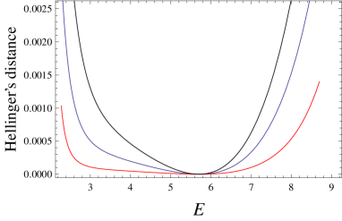
Figure 1: Hellinger’s distance $1-\sum_{k=1}^{4}\sqrt{\hat{p}(y_{k})p(y_{k})}$ between $\hat{p}(y)=\sum_{x}\hat{p}(x,y)$ from (53) and $p(y)$ for $n=m=4$, $p(y)=(0.4,0.01,0.5,0.09)$, $E(x_{k},y_{l})=kl$ ($k,l=1,..,4$) and various values of $E$ that hold (61). From top to bottom: $\beta=0.85$ (black curve), $\beta=0.9$ (blue curve) and $\beta=0.95$ (red curve).

3. We emphasize that the marginal probability $\hat{p}(y)=\sum_{x}\hat{p}(x,y)$ from (53) is generally not equal to $p(y)$, i.e. (45) does not follow from (53). Now $\hat{p}(y)\not=p(y)$ is not prohibited, if $p(y)$ are finite-sample frequencies. But when $N\gg 1$ in (2), then $\hat{p}(y)=p(y)$ is demanded. This equality can be imposed via constraints —additional to (46)—and this will lead to a joint probability different from (53); see Appendix B for details. Instead of imposing additional constraints, we note from (53, 54) that for $\beta<1$ and $\beta\simeq 1$ (written together as $\beta\lesssim 1$), we get $\delta\to 1$, and $\hat{p}(x,y)$ simplifies as

$$\hat{p}(x,y) = p(y)\,\frac{\left[1+\delta-1+\frac{1-\delta}{E}\,E(x,y)\right]^{\frac{1}{\beta-1}}}{\sum_{\bar{x}}\left[1+\delta-1+\frac{1-\delta}{E}\,E(\bar{x},y)\right]^{\frac{\beta}{\beta-1}}}$$ (59)

$$\simeq p(y)\,\frac{e^{-\Gamma E(x,y)}}{\sum_{\bar{x}}e^{-\Gamma E(\bar{x},y)}},$$

$$\Gamma \equiv \frac{1}{E}\,\frac{1-\delta}{1-\beta},$$ (60)

where $\Gamma$ stays finite in the limit $\beta\to 1-0$. It is clear from (59, 60) that in this limit (45) does follow from (53): $\hat{p}(y)=p(y)$; cf. section II.3.

For the present analytically solvable situation, we able to take the the limit $\beta\to 1-0$ and deduce (59, 60). However, upon more general usage of $L_{\beta}$ (and its maximization) this will not be possible, since taking $\beta\approx 1$ in $L_{\beta}$ will run into problems inherited from $L_{1}$ (quasi-degeneracy of maxima etc). Hence it is important to know how close $\beta$ should be to $1$ for recovering $\hat{p}(y)\simeq p(y)$. Fig. (1) illustrates this question by looking at Hellinger’s distance between $\hat{p}(y)$ and $p(y)$. It is seen that $0.9\leq\beta<0.95$ is already sufficient for getting $\hat{p}(y)\simeq p(y)$ sufficiently precisely for almost all values of $E$.

4. Here are finally certain subsidiary, but useful features. When $p(y)$ are the true probabilities of $Y$, then $E$ is supposed to hold the following constraints:

$$\sum_{y}p(y)E(\widetilde{x}(y),y)\leq E\leq\sum_{y}p(y)E(\hat{x}(y),y),$$ (61)

$$\widetilde{x}(y)\equiv{\rm argmin}_{x}[\,E(x,y)\,],\qquad\hat{x}(y)\equiv{\rm argmax}_{x}[\,E(x,y)\,].$$ (62)

In addition, there is a relation that can be deduced directly from (59, 60), but appears to hold more generally, i.e. also for $\beta<1$:

$${\rm sign}\left[\gamma\right]={\rm sign}\left[\frac{1}{n}\sum_{xy}p(y)E(x,y)-E\right].$$ (63)

V Numerical comparison with random choices of nonidentifiable parameters

Table 1: The values of $D_{1}$ and $D_{2}$ given by (resp.) (67) and (68) for $x=1,..,n$ and $y=1,...m=n$ and $E_{1}(x,y)=|x-y|$, $E_{2}(x,y)=xy$. The averaging in (67, 68) was taken over $S=10^{3}$ samples. We took $\beta=0.95$. For completeness, we also presented the analogues of $D_{1}$ and $D_{2}$ (denoted by $K_{1}$ and $K_{2}$, respectively), where Hellinger’s distance in (65) is replaced by the relative entropy: ${\rm dist}[\pi_{k},\hat{p}_{k}]\to\sum_{xy}\pi_{k}(x,y)\ln\frac{\pi_{k}(x,y)}{\hat{p}_{k}(x,y)}$. Both choices support the same conclusion: $D_{1}<D_{2}$, $K_{1}<K_{2}$.

	$n=m=4$	$n=m=5$
$E_{1}$	$D_{1}=0.041$, $D_{2}=0.092$	$D_{1}=0.046$, $D_{2}=0.098$
	$K_{1}=0.145$, $K_{2}=0.410$	$K_{1}=0.153$, $K_{2}=0.442$
$E_{2}$	$D_{1}=0.041$, $D_{2}=0.089$	$D_{1}=0.045$, $D_{2}=0.096$
	$K_{1}=0.143$, $K_{2}=0.434$	$K_{1}=0.155$, $K_{2}=0.430$

In this section we compare predictions obtained from maximizing $L_{\beta<1}$ with the standard attitude of practitioners towards nonidentifiability: people either take a maximum of the (marginal) likelihood $L_{1}$, postulating that if there are many maxima, they are eventually equivalent. Or, within a more careful, but also more laborious approach, they average over sufficiently many such maxima. For the studied model these maxima are given by (45), and the comparison will show that maximizing $L_{\beta\lesssim 1}$ is superior with respect to such random selection methods.

Let us assume that we know the true joint probability $\pi_{k}(x,y)$ of $X$ and $Y$ (the meaning of an integer $k$ is specified below). Given $\pi_{k}(x,y)$ and $E(x,y)$ we calculate the marginal probability of $Y$ and the constraint

$$p_{k}(y)=\sum_{x}\pi_{k}(x,y),\qquad E_{k}=\sum_{xy}E(x,y)\pi_{k}(x,y).$$ (64)

Using (53–55), and $p_{k}(y)$ and $E_{k}$ from (64) we recover $\hat{p}_{k}(x,y)$ that depends on $\beta<1$. Recalling the discussion around (60), we shall work with $\beta=0.95$.

The quality of $\hat{p}_{k}(x,y)$—given by (53–55, 64) as a solution to the problem of estimating $\pi_{k}(x,y)$—can be judged from the distance ${\rm dist}[\pi_{k},\hat{p}_{k}]$, which (for clarity) is chosen to be Hellinger’s distance between two probabilities:

$${\rm dist}[\pi_{k},\hat{p}_{k}]\equiv 1-\sum_{xy}\sqrt{\hat{p}_{k}(x,y)\,\pi_{k}(x,y)}.$$ (65)

Now (65) depends on the choice of $\pi_{k}(x,y)$. To make this dependence weaker, i.e. to make the situation less subjective, we assume that $\pi_{k}(x,y)$ for $k=1,...S\gg 1$ are generated randomly and independently from each other. The simplest possible mechanism suits our purposes: we choose $\Pi_{k}(x,y)$ as $n\times m\times S$ independent random variables homogeneously distributed in $[0,A]$ (the choice of $A$ does not seriously influence on the situation provided that $A\geq 1$), and then calculate:

$$\pi_{k}(x,y)=\Pi_{k}(x,y)\left/{\sum}_{\bar{x}\bar{y}}\right.\Pi_{k}(\bar{x},\bar{y}).$$ (66)

Thus for $S\gg 1$ we define from (65) the averaged distance:

$$D_{1}=\frac{1}{S}\sum_{k=1}^{S}{\rm dist}[\pi_{k},\hat{p}_{k}],$$ (67)

which estimates the quality of $\hat{p}(x,y)$ in predicting the (known) joint probability. To comment on the above choice $\beta=0.95$, we note that from our numeric results that the dependence of $D_{1}$ on $\beta$ is anyhow weak, e.g. it typically changes by 1 % when changing $\beta$ from $0.7$ to $1$.

Now $D_{1}$ will be compared with the situation, where—given $p_{k}(y)$ and $E_{k}$ from (64)— we do not employ (53–55), but instead guess the joint probability of $X$ and $Y$. This will be done by picking up randomly—via the same mechanism, as in (66)—a conditional probability $\widetilde{p}_{k}(x|y)$, with an additional condition that it holds $\sum_{xy}p_{k}(y)\widetilde{p}_{k}(x|y)E(x,y)=E_{k}$ ; see (64). Thereby we construct

$$D_{2}=\frac{1}{S}\sum_{k=1}^{S}{\rm dist}[\pi_{k},p_{k}(y)\widetilde{p}_{k}(x|y)].$$ (68)

Due to $S\gg 1$ in (68), $D_{2}$ is (almost) a sure quantity. Table I compares $D_{2}$ with $D_{1}$ for a representative set of parameters. It is seen that $D_{2}$ is some two times larger than $D_{1}$, i.e. a random solution is worse than (53–55). Table I also shows that $D_{2}>D_{1}$ holds upon using other measures of closeness, e.g. the relative entropy instead of (65).

There is yet another quantity that can be employed for evaluating our approach. Returning to the discussion above (68), we generate independently—following the above recipe, and for a given $\pi_{k}(x,y)$, $p_{k}(y)$ and $E_{k}$—many ($l=1,...,M\gg 1$) conditional probabilities $\widetilde{p}_{k}^{[l]}(x|y)$ that hold $\sum_{xy}p_{k}(y)\widetilde{p}^{[l]}_{k}(x|y)E(x,y)=E_{k}$. Next, we consider the average:

$$\overline{\widetilde{p}}_{k}(x|y)=\frac{1}{M}\sum_{l=1}^{M}\widetilde{p}_{k}^{[l]}(x|y),$$ (69)

which also corresponds to the known practice of taking averages over different outcomes of the likelihood maximization. Eq. (69) is akin to the Bayesian-average estimator, because for given observations (for this case $p_{k}(y)$) it averages over all hidden parameters consistent with the prior information $E_{k}$.

Table 2: The values of $\Delta D_{3}$ given by (70) for $x=1,2,3$, $y=1,2,3$, $E_{1}(x,y)=|x-y|$, and $E_{2}(x,y)=xy$. The averaging in (70) was taken over $S=300$ samples for $M=10^{5}$ in (69). We took $\beta=0.95$. We also presented the analogues of $\Delta D_{3}$ (denoted by $\Delta K_{3}$), where Hellinger’s distance in (70) is replaced by the relative entropy: ${\rm dist}[\pi_{k},\hat{p}_{k}]\to\sum_{xy}\pi_{k}(x,y)\ln\frac{\pi_{k}(x,y)}{\hat{p}_{k}(x,y)}$. Both choices support the same conclusion: $\Delta D_{3}>0$, $\Delta K_{3}>0$.

$E_{1}$	$\Delta D_{3}=0.00278$, $\Delta K_{3}=0.01224$
$E_{2}$	$\Delta D_{3}=0.00215$, $\Delta K_{3}=0.01053$

To understand whether $p_{k}(y)\overline{\widetilde{p}}_{k}(x|y)$ is a better estimate of $\pi_{k}(x,y)$ as compared to $\hat{p}_{k}(x,y)$, we look at averages over independent $\pi_{k}(x,y)$ [cf. (67, 68)]:

$$\Delta D_{3}=\frac{1}{S}\sum_{k=1}^{S}\Delta d_{k},\qquad\Delta d_{k}\equiv{\rm dist}[\pi_{k},p_{k}(y)\overline{\widetilde{p}}_{k}(x|y)]-{\rm dist}[\pi_{k},\hat{p}_{k}(x,y)].$$ (70)

Though particular values of $\Delta d_{k}$ can be negative, the averaged value $\Delta D_{3}>0$ is positive showing that $\hat{p}_{k}(x,y)$ [given by (53)] is a better estimate than $p_{k}(y)\overline{\widetilde{p}}_{k}(x|y)$; see Table 2.

Comparing Table 2 with results of Table I, we see that $p_{k}(y)\overline{\widetilde{p}}_{k}(x|y)$ is closer to $\pi_{k}(x,y)$ than a single random guess $p_{k}(y){\widetilde{p}}_{k}(x|y)$—hence the practical habit of averaging over different outcomes of the maximum-likelihood method does have a rationale in it—but it is still outperformed by $\hat{p}_{k}(x,y)$.

VI Maximizing the generalized likelihood for $\beta>1$

We now turn to maximizing $L_{\beta>1}$ over unknown probabilities $\hat{p}(x,y)$; cf. (44). As seen below, this leads to setting many unknown probabilities to zero, i.e. making the vector $\{\hat{p}(x,y)\}$ sparse. Hence the maximization of $L_{\beta>1}$ does not apply to the problem of solving the observational nonidentifiability, unless this problem comes with a prior information on the sparsity. Even apart of such cases, studying ${\rm max}[\,L_{\beta>1}\,]$ is relevant for those examples, where the maximization of $L_{\beta<1}$ does not provide sufficiently nontrivial result; see section IV.1, where only the marginal probabilities of $X$ and $Y$ are known. As seen below, yet another reason for studying ${\rm max}[\,L_{\beta>1}\,]$ is that it does have close relations with entropy minimization, a technique sporadically employed in probabilistic inference good_entropy ; christensen ; watanabe_entropy (e.g., for the feature extraction problem christensen ) and recently discussed in the context of risk-minimization in decision-making armen .

For simplicity we assume that $N\gg 1$ in (2), i.e. $\sum_{x}\hat{p}(x,y)=p(y)$ holds. Hence we use $\hat{p}(x,y)=\hat{p}(x|y)p(y)$ and write (44) as

$$L_{\beta}=\frac{1}{\beta}\sum_{y}p(y)\ln\left[\sum_{x}\hat{p}^{\beta}(x|y)\right]+\sum_{y}p(y)\ln p(y),$$ (71)

where $\{\hat{p}(x|y)\}$ can be taken as maximization variables. Besides $\sum_{x}\hat{p}(x|y)=1$ and $\hat{p}(x|y)\geq 0$, there can be additional conditions imposed on the maximization, e.g. condition (46). We denote such conditions by ${\cal C}$. Without such constraints, the maximization of (71) is trivial: since $\sum_{x}\hat{p}^{\beta}(x|y)\leq 1$ due to $\beta>1$, the global maximum of (71) is reached for $\hat{p}(x|y)=p_{\rm sparse}(x|y)=\delta_{\rm K}(x,x^{\prime})$, where $\delta_{\rm K}(x,x^{\prime})$ is the Kronecker delta, and where $x^{\prime}$ is an arbitrary value of $X$. Note that the same $p_{\rm sparse}(x|y)$ minimizes the entropy

$$S_{XY}=-\sum_{xy}p(y)\hat{p}(x|y)\ln[p(y)\hat{p}(x|y)],$$ (72)

over $\{\hat{p}(x|y)\}$. In Appendix E we present a numerical evidence that the maximizer of (44) for $\beta>1$ coincides the minimizer of (72) under a nontrivial constraint ${\cal C}$ of the known marginal $p(x)$.

This minimizer corresponds to the possibly majorizing (i.e. in the sense of majorization major ) probability vector under constraints ${\cal C}$; see Appendix D for details. To describe it, one introduces

$$\underset{p(x_{k}|y_{l});\,l=1,...,m,k=1,...,n}{{\rm max}}[\,\hat{p}(x_{k}|y_{l})p(y_{l})\,;{\cal C}].$$ (73)

If the maximization in (73) is reached at $k=k^{*}$ and $l=l^{*}$, then the next element of $\{p(x_{k}|y_{l})\}_{l=1,...,m}^{k=1,...,n}$ is found from:

$$\underset{p(x_{k}|y_{l});\,l=1,...,m,k=1,...,n,\,k\not=k^{*},\,l\not=l^{*}}{{\rm max}}[\,\hat{p}(x_{k}|y_{l})p(y_{l})\,;{\cal C}].$$ (74)

This process continues—taking at each step all previously found elements as contraints—till all elements of $\{p(x|y)\}$ are found. Eqs. (73, 74) emerge as maximizers of a generalized Schur-convex function; see Appendix D. We emphasize that $L_{\beta>1}$ in (71) is not a generalized Schur convex; hence the relation between the maximizer of $L_{\beta>1}$ and (73, 74) is presently an empiric (numeric) fact that needs further understanding.

VII Summary and open problems

How to solve nonidentifiability in parameter determination of mixiture models? We proposed an answer that applies to observational nonidentifiability, where the full model (including hidden variables) is identifiable, but the observed (marginal) model is not; see section II.1. Marginalizing decreases the information available about the unknown parameter(s) cox . This general point can be illustrated by the behavior of the Fisher information that decreases upon marginalizing cox . Here we focus on the extreme case, when the information about the parameter is lost completely. This is the phenomenon of observational nonidentifiability, where the maxima of the marginal likelihood are (infinitely) degenerate. In contrast to most general instances of nonidentifiability (which e.g. can follow from a trivial overparametrization), this particular form is not hopeless to solve, precisely because the full model (including the unobserved or hidden variables) is identifiable.

The presented method amounts to generalizing the marginal likelihood function via $L_{\beta}(\theta)$, where $\theta$ is the unknown parameter(s), and $\beta>0$ is an analogue of inverse temperature from statistical mechanics; see section II.2. For $\beta=1$ we recover the usual marginal likelihood, while $L_{\infty}(\theta)$ amounts to the h-likelihood, where the value of hidden variables is replaced by its MAP (maximum aposteriori) estimate. $L_{\beta}(\theta)$ is constructed by analogy to the statistical physical free energy, where $\beta$ plays the role of inverse temperature; see section II.2. The generalization is motivated by the fact that $L_{\beta}(\theta)$ inherits some of useful features of $L_{1}(\theta)$; see section II.2.

Maximizing $L_{\beta}(\theta)$ instead of $L_{1}(\theta)$ can lead to reasonable predictions if the value of $\beta$ is chosen correctly. We treated several models and argued that the optimal value of $\beta$ is close to, but (strictly) smaller than one. In particular, results predicted by $L_{\beta}(\theta)$ are better than those obtained via what one can call a practitioner’s attitude towards nonidentifiability, i.e. picking up a random maximum of $L_{1}$, or averaging over many such (randomly selected) maxima; see section V. The check was carried out numerically by assuming that the initial data is distributed randomly in a sufficiently unbiased way. We have shown that maximizing $L_{\beta\lesssim 1}(\theta)$ relates to the maximum entropy method; see section II.2.6. Likewise, the maximization of $L_{\beta>1}(\theta)$ relates with minimizing the entropy; see section VI. There are also some analogies between $L_{\beta}(\theta)$ and conditional Renyi entropies renyi1 ; renyi2 .

Several pertinent questions are left open and should motivate further research. (i) Results and methods of section V—that compares predictions of $L_{\beta}(\theta)$ with random selections—should be studied systematically on an analytical base. (ii) How $L_{\beta}(\theta)$ applies to effective nonidentifiability? (iii) Asymptotic analysis of $L_{\beta}(\theta)$ that should link it to a (generalized?) Fisher information. (iv) The relation between maximizing $L_{\beta>1}(\theta)$ and entropy minimization should be clarified; see section VI. So far it is restricted to a perturbation argument (see section II.2.6) and numerical examples; cf. Appendix E. (v) How $L_{\beta}(\theta)$ applies to image restoration problems that also frequently suffer from observational nonidentifiability issues image ?

Appendix A Two alternative approaches

A.1 Bayesian approach to observational nonidentifiability

Here we outline a Bayesian approach to the observationally nonidentifiable model discussed in section II.3. First of all, recall from (27) that $p_{gh}(x,y)=p(x,y|g,h)$ is a conditional probability. Given an observation $Y=y$ we want to exclude the parameter $h$ so as to gain information on the parameter $g$ via a conditinal probability $p(g|y)$. To this end, we have to come up with prior probabilities of $h$ and $g$. We make the simplest assumption that a priori they are independent: $p(h,g)=p(h)p(g)$ and that the prior $p(h)$ is noninformative. In the Bayesian approach this means that we have to take jaynes (depending on the possible range of $h$):

$$p(h)\propto 1\qquad{\rm if}\qquad\infty>h>-\infty,$$ (75)

$$p(h)\propto 1/h\qquad{\rm if}\qquad\infty>h>0.$$ (76)

Note that both priors probability densities (75, 76) are improper, i.e. they are not normalizable. Improper priors can still lead to useful applications jaynes .

The first step in calculating $p(g|y)$ is to study $p(x,y|g)$ from (27) and (75)

$$p(x,y|g)\overset{?}{\propto}\int{\rm d}h\,p(x,y|g,h)p(h).$$ (77)

Now (75, 76) and (27) show that the integral in the right-hand-side of (77) does not exist, i.e. the Bayesian approach with non-informative priors is blocked already at its first step. If a proper prior is available instead of (75, 76), then the Bayesian approach does work. We do not dwell into this, since we assume that no prior information is available.

A.2 Decision theory approach: attempts to build a maximin estimator for an observationally non-identifiable model

Following the basic tenets of the decision theory approach cox , we shall attempt to build a maximin estimator for the model model discussed in section II.3. The virtue of such an estimator is that its construction does not need prior probabilities for unknown parameters cox .

Starting from (27, 28) and assuming that $y$ is observed we construct

$${\rm dist}[p_{\hat{g}(y)\,\hat{h}(y)}(x|y),p_{gh}(x|y)]=1-\sum_{x}\sqrt{p_{\hat{g}(y)\,\hat{h}(y)}(x|y)p_{gh}(x|y)}$$ (78)

$$=1-\frac{\cosh\left[\frac{g+\hat{g}(y)}{2}+\frac{y(h+\hat{h}(y))}{2}\right]}{\sqrt{\cosh\left[g+yh\right]\,\cosh\left[\hat{g}(y)+y\hat{h}(y)\right]}},$$ (79)

where the choose to work with Hellinger’s distance, and where $\hat{g}(y)$ and $\hat{h}(y)$ are estimators of (resp.) $g$ and $h$ given the observation $y$. Together with (78), one also employs the distance, which is averaged over observations cox :

$$\sum_{y}p_{gh}(y)\,{\rm dist}[p_{\hat{g}(y)\,\hat{h}(y)}(x|y),p_{gh}(x|y)]$$ (80)

$$=1-\frac{\cosh[u]}{\cosh[u]+\cosh[v]}\,\frac{\cosh[(u+\widetilde{u})/2]}{\sqrt{\cosh[u]\cosh[\widetilde{u}]}}-\frac{\cosh[v]}{\cosh[u]+\cosh[v]}\,\frac{\cosh[(v+\widetilde{v})/2]}{\sqrt{\cosh[v]\cosh[\widetilde{v}]}},$$ (81)

where in (81) we defined

$$u\equiv h+g>0,\qquad v\equiv h-g,\qquad\widetilde{u}\equiv\hat{h}(1)+\hat{g}(1)>0,\qquad\widetilde{v}\equiv\hat{h}(-1)-\hat{g}(-1).$$ (82)

Note that the constraints $u>0$ and $\widetilde{u}>0$ come from our assumption on $g>0$ and $h>0$.

The maximin estimator takes the worst case (i.e. the maximal distance) with respect to unknown parameters $g$ and $h$, and then minimizes this worst case over the estimators $\hat{h}(y)$ and $\hat{g}(y)$ cox . In principle, this procedure can be applied to either (79) or (81). We shall start by applying it to (79). We note from (79, 82):

$$1-{\rm dist}[p_{\hat{g}(y)\,\hat{h}(y)}(x|1),p_{gh}(x|1)]=\frac{\cosh[(u+\widetilde{u})/2]}{\sqrt{\cosh[u]\cosh[\widetilde{u}]}},$$ (83)

$$1-{\rm dist}[p_{\hat{g}(y)\,\hat{h}(y)}(x|-1),p_{gh}(x|-1)]=\frac{\cosh[(v+\widetilde{v})/2]}{\sqrt{\cosh[v]\cosh[\widetilde{v}]}}.$$ (84)

The first step amounts to maximizing the distance over unknown $g$ and $h$, i.e. over $u>0$ and $v$:

$${\rm min}_{u>0}\,\frac{\cosh[(u+\widetilde{u})/2]}{\sqrt{\cosh[u]\cosh[\widetilde{u}]}} = \frac{e^{\widetilde{u}/2}}{\sqrt{2\cosh\widetilde{u}}}\quad{\rm for}\quad\widetilde{u}<-\ln[\sqrt{2}-1],$$ (85)

$$= \frac{\cosh[\widetilde{u}/2]}{\sqrt{\cosh\widetilde{u}}}\quad{\rm for}\quad\widetilde{u}>-\ln[\sqrt{2}-1],$$ (86)

$${\rm min}_{v}\,\frac{\cosh[(v+\widetilde{v})/2]}{\sqrt{\cosh[v]\cosh[\widetilde{v}]}} = \frac{e^{-|\widetilde{v}|/2}}{\sqrt{2\cosh\widetilde{v}}},$$ (87)

where the last relation is deduced for $v\to\pm\infty$ depending on the sign of $\widetilde{v}$.

At the second step we should minimize the distance over estimators, i.e. (85, 86) is to be maximized over $\widetilde{u}$, while (87) is to be maximized over $\widetilde{v}$. This step is supposed to define those estimators. We get from (85–87):

$$\widetilde{u}=0,\infty,$$ (88)

$$\widetilde{v}=0,$$ (89)

where the two values $0$ or $\infty$ for $\widetilde{u}$ in (88) come from (resp.) (85) and (86). While $\widetilde{v}=0$ in (89) seems reasonable (though incomplete) value for the estimator, neither of $\widetilde{u}=0$ or $\widetilde{u}=\infty$ is meaningful. Hence the maximin strategy applied to (79) does not leas to sensible estimators.

When applying the strategy to (81), we note that (87)$\leq$(85) and (87)$\leq$(86) for all allowed values of $\widetilde{u}$ and $\widetilde{v}$. Hence we find

$${\rm min}_{u>0,\,v}\left[\frac{\cosh[u]}{\cosh[u]+\cosh[v]}\,\frac{\cosh[(u+\widetilde{u})/2]}{\sqrt{\cosh[u]\cosh[\widetilde{u}]}}-\frac{\cosh[v]}{\cosh[u]+\cosh[v]}\,\frac{\cosh[(v+\widetilde{v})/2]}{\sqrt{\cosh[v]\cosh[\widetilde{v}]}}\right]=\frac{e^{-|\widetilde{v}|/2}}{\sqrt{2\cosh\widetilde{v}}},$$ (90)

where the last relation is again deduced for $v\to\pm\infty$. The maximization of (90) over $\widetilde{v}$ brings us sback to (89). Again nothing reasonable is produced for $\widetilde{u}$: the maximin method does not work for this example.

Appendix B Maximization of $L_{\beta}$ under two constraints

Consider the maximization of $L_{\beta}$ given by (44) under two constraints [cf. section IV.2]

$$\sum_{x}\hat{p}(x,y)=p(y),\qquad\sum_{xy}E(x,y)\hat{p}(x,y)=E,$$ (91)

where $E(x,y)$ is a function of $x$ and $y$ with a known average $E$. The Lagrange function reads:

$${\cal L}_{\beta}=\frac{1}{\beta}\sum_{y}p(y)\ln\left[\sum_{x}\hat{p}^{\beta}(x,y)\right]-\sum_{xy}\delta(y)\hat{p}(x,y)-\gamma\sum_{xy}E(x,y)\hat{p}(x,y),$$ (92)

where $\delta(y)$ and $\gamma$ refer to (resp.) (91) and (91). Now $\frac{\partial{\cal L}_{\beta}}{\partial\hat{p}(x,y)}=0$ leads to

$$\frac{p(y)\hat{p}^{\beta-1}(x,y)}{\sum_{\bar{x}}\hat{p}^{\beta}(\bar{x},y)}=\delta(y)+\gamma E(x,y),$$ (93)

which is solved as

$$\hat{p}(x,y)=p(y)\,\frac{\left[\delta(y)+\gamma E(x,y)\right]^{\frac{1}{\beta-1}}}{\sum_{\bar{x}}\left[\delta(y)+\gamma E(\bar{x},y)\right]^{\frac{\beta}{\beta-1}}}.$$ (94)

Here $\delta(y)$ and $\gamma$ are found from (resp.) (91) and (91). Eventually, $\gamma$ can be expressed via $\delta(y)$, which is found from (96):

$$\gamma=\frac{1}{E}\left(1-\sum_{y}p(y)\delta(y)\right),$$ (95)

$$\sum_{x}{\left[\delta(y)+\gamma E(x,y)\right]^{\frac{1}{\beta-1}}}={\sum_{{x}}\left[\delta(y)+\gamma E(x,y)\right]^{\frac{\beta}{\beta-1}}}.$$ (96)

Appendix C The relevance of various constraints in the maximum entropy method

The maximum entropy method addresses the problem of recovering unknown probabilities $\{q(z_{k})\}_{k=1}^{n}$ of a random variable $Z=(z_{1},...,z_{n})$ via maximization of the entropy

$$S[q]=-\sum_{k=1}^{n}q(z_{k})\ln q(z_{k}).$$ (97)

subject to certain constraints on $q$ and $Z$ jaynes ; jaynes_2 ; skyrms ; enk ; cheeseman . These constraints are assumed to come as a prior information, within its standard formulation the method does not determine the type and a number of those constraints; the only (obvious) requirement from the method is that the result of maximization is unique. The intuitive rationale of the method is that provides the most unbiased choice of probability compatible with the constraints.

One way of recovering the constraints is to look at (necessarily noisy) data. If this way is followed in detail, it can give some recommendations on selecting the constraints, or at least on determining their relative relevance. Below we shall present some preliminary results to this effect within. Since the results are preliminary, we shall not attempt to generalize them towards the likelihood $L_{\beta<1}$.

A standard way of checking an inference method is to assume that the true probabilities are known. Hence we shall start by assuming that we know the probabilities $\{q(z_{k})\}_{k=1}^{n}$ of $Z=(z_{1},...,z_{n})$. From $\{q(z_{k})\}_{k=1}^{n}$ we generate a finite i.i.d. sample

$${\cal S}_{M}=(z_{i_{1}},...,z_{i_{M}})$$ (98)

of length $M$. Various constraints are now to be recovered from (98). Here are several examples

– We can apply no constraint at all and just maximize the entropy:

$$q^{[0]}(z_{k})=\frac{1}{n}.$$ (99)

– After calculating the empiric mean of (98),

$$\mu=\frac{1}{M}\sum_{u=1}^{M}z_{i_{u}},$$ (100)

we can take it as an estimate for the true average $\sum_{k=1}^{n}q(z_{k})z_{k}$, and recover approximate probabilities $\{q^{[1]}(z_{k})\}_{k=1}^{n}$ via maximizing (97) subject to a constraint: $\sum_{k=1}^{n}q^{[1]}(z_{k})z_{k}=\mu$. It is well-known jaynes ; jaynes_2 that this maximization leads to

$$q^{[1]}(z_{k})=\frac{e^{-\beta z_{k}}}{\sum_{l}e^{-\beta z_{l}}},$$ (101)

where $\beta$ is determined from $\sum_{k=1}^{n}q^{[1]}(z_{k})z_{k}=\mu$.

– The empiric means is certainly not the only information contained in the sample; e.g. one can estimate as well the second moment:

$$\mu_{2}=\frac{1}{M}\sum_{u=1}^{M}z^{2}_{i_{u}},$$ (102)

and maximize (97) under two contraints (100) and (102):

$$q^{[1+2]}(z_{k})=\frac{e^{-\beta_{1}z_{k}-\beta_{2}z_{k}^{2}}}{\sum_{l}e^{-\beta_{1}z_{l}-\beta_{2}z_{l}^{2}}},$$ (103)

where $\beta_{1}$ and $\beta_{2}$ are determined from $\sum_{k=1}^{n}q^{[1+2]}(z_{k})z_{k}=\mu$ and $\sum_{k=1}^{n}q^{[1+2]}(z_{k})z_{k}^{2}=\mu_{2}$.

– It is the standard lore of statistics that for relatively short samples, the empiric median is a better (more robust) estimator than the empiric mean. Thus we should pay attention to the median as a constraint in the entropy maximization. Recalling the definition of the median ${\rm Md}$ for given (discrete-variable) probabilities, the maximum of (97) under a fixed median is made obvious with the following example for $n=4$ (assuming for simplicity that $z_{1}<z_{2}<z_{3}<z_{4}$):

$${\rm Md}=z_{1}:\quad{\rm argmax}_{q}[\,S[q]\,]=\frac{1}{2}\left(1+\epsilon,\frac{1-\epsilon}{3},\frac{1}{3},\frac{1}{3}\right),$$ (104)

$${\rm Md}=z_{2}:\quad{\rm argmax}_{q}[\,S[q]\,]=\frac{1}{2}\left(\frac{1}{2},\frac{1+\epsilon}{2},\frac{1-\epsilon}{2},\frac{1}{2}\right),$$ (105)

$${\rm Md}=z_{3}:\quad{\rm argmax}_{q}[\,S[q]\,]=\frac{1}{2}\left(\frac{1}{3},\frac{1}{3},\frac{1+\epsilon}{3},1-\epsilon\right),$$ (106)

$${\rm Md}=z_{4}:\quad{\rm argmax}_{q}[\,S[q]\,]=\frac{1}{2}\left(\frac{1}{3},\frac{1}{3},\frac{1-\epsilon}{3},1+\epsilon\right),$$ (107)

where $\epsilon>0$ is infinitely small. We kept it for confirming that the median is indeed equal to its fixed value, but $\epsilon$ can be neglected in actual calculations. Eqs. (104–107) easily generalize to an arbitrary finite $n$.

Now the median ${\rm Md}$ will estimated from the finite sample (as an empiric median), and the maximum entropy probabilities recovered according to (104–107) will be denoted as $\{q^{\rm[md]}(z_{k})\}_{k=1}^{n}$

We can calculate how close are the above estimates from the true probabilities $q=\{q(z_{k})\}_{k=1}^{n}$:

$$d_{0}={\rm dist}[q^{[0]},q],\quad d_{1}={\rm dist}[q^{[1]},q],\quad d_{1+2}={\rm dist}[q^{[1+2]},q],\quad d_{\rm md}={\rm dist}[q^{[{\rm md}]},q],$$ (108)

where ${\rm dist}[.,.]$ can be e.g. the Hellinger distance:

$${\rm dist}[q^{[0]},q]\equiv 1-\sum_{k=1}^{n}\sqrt{q(z_{k})\,q^{[0]}(z_{k})}.$$ (109)

Besides $d_{0}$, quantities defined in (108) are random variables together with the sample (98). Hence we shall average them over ${\cal M}\gg 1$ independently generated samples, keeping the sample length $M$ fixed. The averaged quantities will be denoted as

$$\langle d_{1}\rangle,\quad\langle d_{1+2}\rangle,\quad\langle d_{\rm md}\rangle.$$ (110)

Together with $d_{0}$ they depend on $q=\{q(z_{k})\}_{k=1}^{n}$. Besides quantities in (110) we shall also study their averages over $q=\{q(z_{k})\}_{k=1}^{n}$: we generate randomly ${\cal N}$ probabilities (the mechanism for this is discussed in section V of the main text), and average $\langle d_{1}\rangle$, $\langle d_{1+2}\rangle$, $\langle d_{\rm md}\rangle$, and $d_{0}$ over them. The results will be denoted by

$$\overline{d}_{1},\quad\overline{d}_{1+2},\quad\overline{d}_{\rm md},\quad\overline{d}_{0}.$$ (111)

Table 3 presents a numerical illustration for quantities defined in (108–111). It is seen that when $M$ is larger, but comparable to $n$ ($M=7$ and $n=6$ in Table 3), the situation is so noisy that samples do not provide information from the viewpoint of the constraints studied . This means that the no-constraint solution (99) is always better because in the majority of cases we get ${\rm min}[\langle d_{1}\rangle,\langle d_{1+2}\rangle,\langle d_{\rm md}\rangle,d_{0}]=d_{0}$, and because ${\rm min}[\overline{d}_{1},\overline{d}_{1+2},\overline{d}_{\rm md},\overline{d}_{0}]=\overline{d}_{0}$. For such values of $M$ employing the above constrained solutions will just amount to an overfitting (of noise).

For a larger $M$ ($M=11$ and $n=6$ in Table 3), we see that (101) is the best constraint in one sense, since now the solution (101) provides a smaller average distance from the true solution: ${\rm min}[\overline{d}_{1},\overline{d}_{1+2},\overline{d}_{\rm md},\overline{d}_{0}]=\overline{d}_{1}$. However, in the second sense (99) is still better, because the percentage of cases, where ${\rm min}[\langle d_{1}\rangle,\langle d_{1+2}\rangle,\langle d_{\rm md}\rangle,d_{0}]=d_{0}$ is still the largest one. Applying the median solution or the second-order solution (103) lead to worse results. Table 3 shows that the solution based on the median is always worse than some of the other solutions.

The second-order solution (103) becomes the best solution for $M\geq 21$; see Table 3. This holds in terms of the average distance: ${\rm min}[\overline{d}_{1},\overline{d}_{1+2},\overline{d}_{\rm md},\overline{d}_{0}]=\overline{d}_{1+2}$, and also in terms of the percentage of cases, where ${\rm min}[\langle d_{1}\rangle,\langle d_{1+2}\rangle,\langle d_{\rm md}\rangle,d_{0}]=d_{1+2}$. Increasing $M$ more just confirms this trend, i.e. improves the quality of (103) in both senses. Interestingly, the percentage of cases, where ${\rm min}[\langle d_{1}\rangle,\langle d_{1+2}\rangle,\langle d_{\rm md}\rangle,d_{0}]=d_{1}$ is relatively stable for larger values of $M$: in more than $1/6$ of cases the first-order solution (101) is still better than other solutions, even for $M=101$; see Table 3.

Our (preliminary) conclusions are summarized as follows: (i) The median is not a relevant constraint for the maximum entropy method. It is never better than the average. (ii) The latter solution does overfit for short samples ($M\simeq n$), where having no constraints whatsoever is better than fixing the average. (iii) For sufficiently long samples fixing the first and second moments outperforms other solutions, but the average constraint does stay reasonable even for larger sample lengths.

$M$	$\%\,{\rm min}=\langle d_{1}\rangle$	$\%\,{\rm min}=\langle d_{1+2}\rangle$	$\%\,{\rm min}=\langle d_{\rm med}\rangle$	$\%\,{\rm min}=d_{0}$	$\overline{d}_{1}$	$\overline{d}_{1+2}$	$\overline{d}_{\rm md}$	$\overline{d}_{0}$
7	18	4	8	70	0.06194	0.07713	0.06771	0.05535
11	25	18	7	50	0.05548	0.05829	0.06212	0.05656
21	24	41	2	33	0.04731	0.04421	0.05894	0.05350
31	27	45	1	27	0.04583	0.04125	0.05935	0.05520
41	29	51	2	18	0.05091	0.04302	0.06311	0.05970
61	24	64	2	10	0.04628	0.03531	0.05459	0.05430
101	18	71	0	11	0.04296	0.03567	0.05519	0.05179

Table 3: For a set-up of a dice: $n=6$ and $z_{k}=k$ ($k=1,...,6$) we show various quantities defined above and below (108). The ${\rm dist}[.,.]$ in (108) was chosen to be the Hellinger distance. $M$ is the number of samples. The average in (110) is defined over $10^{4}$ indepedent samples generated via the method described in section V. The average in (111) is defined over $100$ realizations of probabilities. Now $\%\,{\rm min}=\langle d_{1}\rangle$ means the percentage of the relation $\%\,{\rm min}[\langle d_{1}\rangle,\langle d_{1+2}\rangle,\langle d_{\rm md}\rangle,d_{0}]=d_{1}$ among those $100$ cases; e.g. $\%\,{\rm min}=\langle d_{1}\rangle\to 18$ means that in 18 cases out of 100 we got ${\rm min}[\langle d_{1}\rangle,\langle d_{1+2}\rangle,\langle d_{\rm md}\rangle,d_{0}]=\langle d_{1}\rangle$. The minimal among $\overline{d}_{1}$, $\overline{d}_{1+2}$, $\overline{d}_{\rm md}$, and $\overline{d}_{0}$ is underlined.

Appendix D Generalized Schur-convexity

We shall briefly review implications of the generalized Schur-convexity major for maximizing functions similar to (71). Though we were not able to show that (71) is generalized Schur-convex, numerical results show the Schur-convex maximizers provide a good description of local maxima for (71).

Let we are given a differentiable function $\Phi(x;u)$ of two vectors: $x=(x_{1},...,x_{M})$ and $u=(u_{1},...,u_{M})$. Both vary on compact subsets of $\mathfrak{R}^{M}$, and $u_{k}\not=0$ for all $k=1,...,M$. Let us assume that $\Phi(x;u)$ is Schur-convex major :

$$(x_{k}-x_{l})\left[\frac{1}{u_{k}}\frac{\partial\Phi}{\partial x_{k}}-\frac{1}{u_{l}}\frac{\partial\Phi}{\partial x_{l}}\right]\geq 0,\qquad k,l=1,..,M-1.$$ (112)

Let ${\cal D}$ be the set of vectors that are ordered as: $x_{1}\geq...\geq x_{M}$. Denote

$$z_{\ell}\equiv\sum_{k=1}^{\ell}u_{k}x_{k},\quad\ell=1,...,M,$$ (113)

and note that $\Phi(x;u)$ can be written as

$$\Phi(x;u)=\Phi(\,\frac{z_{1}}{u_{1}},\frac{z_{2}-z_{1}}{u_{2}},...,\frac{z_{M}-z_{M-1}}{u_{M}}\,;u)\equiv\widetilde{\Phi}(z_{1},...,z_{M}).$$ (114)

Now for $x\in{\cal D}$, $\widetilde{\Phi}(z_{1},...,z_{M})$ is a non-decreasing function of $z_{1}$, … $z_{M-1}$, because then (112) reduces to

$$\frac{1}{u_{k}}\frac{\partial\Phi}{\partial x_{k}}-\frac{1}{u_{k+1}}\frac{\partial\Phi}{\partial x_{k+1}}\geq 0,\qquad k=1,..,M-1,$$ (115)

and then (115) implies

$$\frac{\partial\widetilde{\Phi}}{\partial z_{k}}\geq 0\quad{\rm for}\quad k=1,...,M-1\quad{\rm and}\quad x\in{\cal D}.$$ (116)

Let us denote by ${\cal A}$ the set of all vectors $x$ that hold

$$\sum_{k=1}^{M}u_{k}x_{k}=1.$$ (117)

Eq. (116) will show how to maximize $\Phi(x;u)$ over $x\in{\cal A}\cap{\cal D}$. First consider two vectors, $x\in{\cal D}\cap{\cal A}$ and $y\in{\cal D}\cap{\cal A}$. Eq. (113) and conditions (116) imply that if:

$$\sum_{k=1}^{\ell}u_{k}x_{k}\geq\sum_{k=1}^{\ell}u_{k}y_{k},\quad\ell=1,...,M-1,$$ (118)

then

$$\Phi(x;u)\geq\Phi(y;u).$$ (119)

Eqs. (112, 118) refer to the concept of $u$-majorization, while $\Phi(x;u)$ in (119) is a $u$-Schur-convex function major .

Now ${\rm argmax}_{x\in{\cal A}\cap{\cal D}}[\,\Phi(x,u)\,]$ is found as follows: one first finds ${\rm max}_{x_{1}\in{\cal A}\cap{\cal D}}[\,u_{1}x_{1}\,]$. Then taking this maximized value as a condition one obtains ${\rm max}_{x_{2}\in{\cal A}\cap{\cal D}}[\,u_{2}x_{2}\,]$, then under two previous conditions one finds ${\rm max}_{x_{3}\in{\cal A}\cap{\cal D}}[\,u_{3}x_{3}\,]$ etc.

We generalize the above reasoning taking instead of ${\cal D}$ any other ordering: $x\in{\cal D}^{\pi}$ means that $x_{\pi_{1}}\geq...\geq x_{\pi_{M}}$, where $\pi$ is a certain permutation of indices $1,...,M$. Conditions (112, 117) stay without changes.

To obtain $x^{*}\equiv{\rm argmax}_{x\in{\cal A}}[\,\Phi(x,u)\,]$ under (112) and (117) (i.e. without imposing any condition $x\in{\cal D}^{\pi}$ for a specific $\pi$), we shall optimize the above construction over all possible ${\cal D}^{\pi}$. Thus one first finds

$$\underset{1\leq k\leq M}{\rm max}\,\underset{x\in{\cal A}}{\rm max}[\,u_{k}x_{k}\,].$$ (120)

If this maximum is reached at a certain value $x_{j_{1}}^{*}$ of $x_{j_{1}}$, then one looks at

$$\underset{1\leq k\leq M,k\not=j_{1}}{\rm max}\,\underset{x\in{\cal A}}{\rm max}[\,u_{k}x_{k}\,].$$ (121)

If the maximum in (121) is reached at a certain value $x_{j_{2}}^{*}$ of $x_{j_{2}}$, then the next maximization excludes both $j_{1}$ and $j_{2}$; and so on till all elements of $x^{*}\in{\cal A}$ will be found.

Returning to the problem stated by the maximization of (71), we note that the index $k$ in (117, 115) corresponds to the double index $(x,y)$, where $M=nm$, while $x$ and $u$ refer to $\{\hat{p}(x|y)\}_{x,y}$ $\{p(y)\}_{x,y}$, respectively. Eq. (117) then holds due to normalization. Likewise, ${\cal A}$ is defined from relevant constraints, e.g. from (47). But conditions (112) for $L_{\beta>1}$ do not hold, since the left-hand-side of (112) amounts to

$$\left[\hat{p}(x|y)-\hat{p}(x^{\prime}|y^{\prime})\right]\left(\frac{\hat{p}^{\beta-1}(x|y)}{\sum_{\bar{x}}\hat{p}^{\beta}(\bar{x}|y)}-\frac{\hat{p}^{\beta-1}(x^{\prime}|y^{\prime})}{\sum_{\bar{x}}\hat{p}^{\beta}(\bar{x}|y^{\prime})}\right),$$ (122)

which is generally not nonnegative. In contrast, the negative average entropy: $\sum_{y}p(y)\sum_{x}\hat{p}(x|y)\ln\hat{p}(x|y)$ does hold (112):

$$\left[\hat{p}(x|y)-\hat{p}(x^{\prime}|y^{\prime})\right]\left[\ln\hat{p}(x|y)-\ln\hat{p}(x^{\prime}|y^{\prime})\right]\geq 0.$$ (123)

Appendix E Maximization of $L_{\beta>1}$ for known marginals of $X$ and $Y$ illustrated via examples

There are infinitely many joint probabilities $\hat{p}(x,y)$ with given marginals $p(y)$ and $p(x)$ copulas ; cohen_zap ; finch . One can ask about the simplest joint probabilities compatible with given marginals good ; kullback . Such a probability can be employed as a null-hypothesis and serve as a starting point for further approximations. It is well-known that the maximal entropy reasoning leads to the factorized joint probability $\hat{p}(x,y)=p(x)p(y)$ good , which we also got from maximizing $L_{\beta<1}$; see section IV.1. Below we show numerically that the maximization of $L_{\beta>1}$ leads to a different and unique prediction for $\hat{p}(x,y)$ that agrees with (73, 74). Hence it agrees with minimizing the joint entropy (72) under the constraint of given marginals. This is a well-known problem, because (for given marginals) it is equivalent to maximizing the mutual information between $X$ and $Y$; see min_entropy_marg_1 ; min_entropy_marg_2 ; min_entropy_marg_3 for recent discussions.

Let us assume that both $X$ and $Y$ assume 3 values $(x_{1},x_{2},x_{3})$ and $(y_{1},y_{2},y_{3})$, respectively. Here is an example for the (global) maximizer of (71) that we presented in the form of (47) with numeric values of $\hat{p}(x|y)$ written in bold:

$$(\,p(y_{1}),p(y_{2}),p(y_{3})\,)=(0.1,0.3,0.6),$$ (124)

$$p(x_{1})=0.55={\bf 0}\times 0.1+{\bf 0}\times 0.3+{\bf\frac{55}{60}}\times 0.6,$$ (125)

$$p(x_{2})=0.25={\bf 0}\times 0.1+{\bf\frac{25}{30}}\times 0.3+{\bf 0}\times 0.6,$$ (126)

$$p(x_{3})=0.20={\bf 1}\times 0.1+{\bf\frac{5}{30}}\times 0.3+{\bf\frac{5}{60}}\times 0.6.$$ (127)

Eqs. (125–127) follow (73, 74). First one finds $\hat{p}(x_{1}|y_{3})=55/60$, since this provides the largest possible value for the joint probability: $\hat{p}(x_{1},y_{3})=0.5$. Due to (125) this already sets $\hat{p}(x_{1}|y_{1})=\hat{p}(x_{1}|y_{2})=0$. Next, one finds $\hat{p}(x_{2}|y_{2})=25/30$, since this provides the second-largest value of the joint probability, $\hat{p}(x_{2}|y_{2})=0.25$, also enforcing $\hat{p}(x_{2}|y_{1})=\hat{p}(x_{2}|y_{3})=0$. Remaining $p(x|y)$ in (127) are recovered from normalization.

It is seen that $\hat{p}(x|y)$ given in (125–127) do have the maximal number of zeroes (4 for the considered case $n=m=3$) allowed by (47). I.e. the maximizers of $L_{\beta>1}$ are located at vertices of the convex domain (47).

The second example is dealt with in the same way with $\hat{p}(x_{1}|y_{1})=4/9$ being the first step, and $\hat{p}(x_{3}|y_{2})=\hat{p}(x_{3}|y_{3})=1$ amount to the last step:

$$(p(y_{1}),p(y_{2}),p(y_{3}))=(0.9,0.06,0.04),$$ (128)

$$p(x_{1})=0.4={\bf\frac{4}{9}}\times 0.9+{\bf 0}\times 0.06+{\bf 0}\times 0.04,$$ (129)

$$p(x_{2})=0.35={\bf\frac{35}{90}}\times 0.9+{\bf 0}\times 0.06+{\bf 0}\times 0.04,$$ (130)

$$p(x_{3})=0.25={\bf\frac{15}{90}}\times 0.9+{\bf 1}\times 0.06+{\bf 1}\times 0.04.$$ (131)

The maximizers (but not the value of $L_{\beta}$) do not depend on $\beta$ provided that $\beta>1$. However, we noted that for $\beta\to\infty$ the global maximum of $L_{\beta}$ are difficult to reach numerically, since they are plagued by many local maxima. Hence employing moderate values of $\beta$ (e.g. $\beta=2$) can be beneficial for finding the global maximum numerically. This point can be illustrated by comparing the global maximizer (129–131) with

$$(p(y_{1}),p(y_{2}),p(y_{3}))=(0.9,0.06,0.04),$$ (132)

$$p(x_{1})=0.4={\bf\frac{4}{9}}\times 0.9+{\bf 0}\times 0.06+{\bf 0}\times 0.04,$$ (133)

$$p(x_{2})=0.35={\bf\frac{29}{90}}\times 0.9+{\bf 1}\times 0.06+{\bf 0}\times 0.04,$$ (134)

$$p(x_{3})=0.25={\bf\frac{21}{90}}\times 0.9+{\bf 0}\times 0.06+{\bf 1}\times 0.04.$$ (135)

Both (129–131) and (133–135) produce the same value for $L_{\beta\to\infty}$, because

$$L_{\beta\to\infty}=\sum_{y}p(y)\ln\left[\hat{p}(\widetilde{x}(y)|y)\right]+\sum_{y}p(y)\ln p(y),\qquad\widetilde{x}(y)\equiv{\rm argmax}_{x}[\,p(x|y)\,].$$ (136)

Indeed, both (129–131) and (133–135) have the same values of $\hat{p}(\widetilde{x}(y)|y)$. Even though the global maximum of $L_{\beta>1}$ may be difficult to reach numerically, we noted that numerically reachable local maxima also have the same (i.e. maximal) number of zeros.