Lake Ice Monitoring with Webcams and Crowd-Sourced Images

Abstract

Lake ice is a strong climate indicator and has been recognised as part of the Essential Climate Variables (ECV) by the Global Climate Observing System (GCOS). The dynamics of freezing and thawing, and possible shifts of freezing patterns over time, can help in understanding the local and global climate systems. One way to acquire the spatio-temporal information about lake ice formation, independent of clouds, is to analyse webcam images. This paper intends to move towards a universal model for monitoring lake ice with freely available webcam data. We demonstrate good performance, including the ability to generalise across different winters and lakes, with a state-of-the-art Convolutional Neural Network (CNN) model for semantic image segmentation, Deeplab v3+. Moreover, we design a variant of that model, termed Deep-U-Lab, which predicts sharper, more correct segmentation boundaries. We have tested the model’s ability to generalise with data from multiple camera views and two different winters. On average, it achieves Intersection-over-Union (IoU) values of $\approx$71% across different cameras and $\approx$69% across different winters, greatly outperforming prior work. Going even further, we show that the model even achieves 60% IoU on arbitrary images scraped from photo-sharing websites. As part of the work, we introduce a new benchmark dataset of webcam images, Photi-LakeIce, from multiple cameras and two different winters, along with pixel-wise ground truth annotations.

1 INTRODUCTION

Climate change is and will continue to be, a main challenge for humanity. In the words of Stephen Haddrill (2014), "Climate change is a reality that is happening now, and that we can see its impact across the world". Lakes play an essential role in the quest to monitor and better understand the climate system. One important piece of information about lakes in cooler climate zones are the times, duration and patterns of freezing and thawing. Long-term changes and shifts of these variables mirror changes in the local climate. Therefore, there is a need to analyse the temporal dynamics of lake ice, and in fact, it has been designated an ECV by the GCOS.

This work explores the potential of webcam images, in conjunction with modern semantic segmentation algorithms such as Deeplab v3+ (Chen et al.,, 2018), for lake ice monitoring. The goal is to construct a spatially resolved time series of the spatio-temporal extent of lake ice (note that coarser indicators, e.g., the ice-on and ice-off dates, can easily be derived from the time series). Given the promising results of Deeplab v3+ on other semantic segmentation tasks such as PASCAL VOC (Everingham et al.,, 2015) and Cityscapes (Cordts et al.,, 2016), we base our approach on that model.

The core task for the envisaged monitoring system is: in every camera frame, classify each pixel capturing the lake surface as water, ice, snow and clutter, i.e., other objects on the lake, mostly due to human activity such as tents, boats etc. See Fig. 1c. With a view towards a future operational system, we do lake detection, followed by fine-grained classification. See Fig. 1b. In both steps we take advantage of transfer learning and employ models pre-trained on external databases (here, the PASCAL VOC dataset), to compensate for the relative scarcity of annotated data.

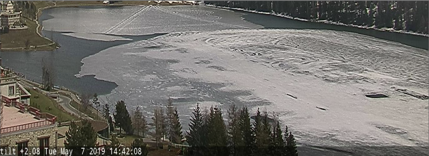
(a) Webcam RGB image

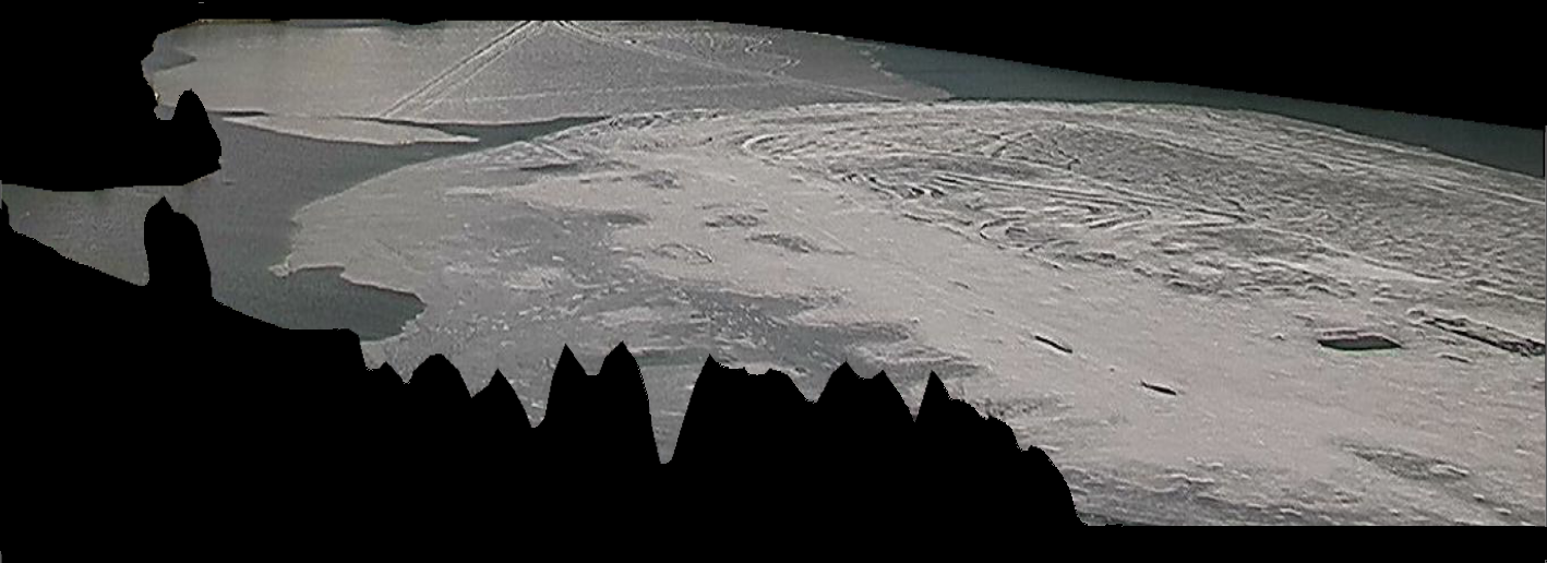
(b) Lake detection

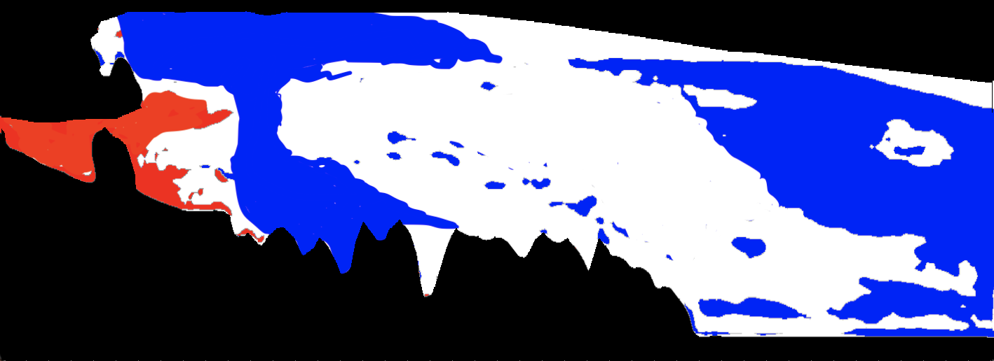
(c) Lake ice segmentation

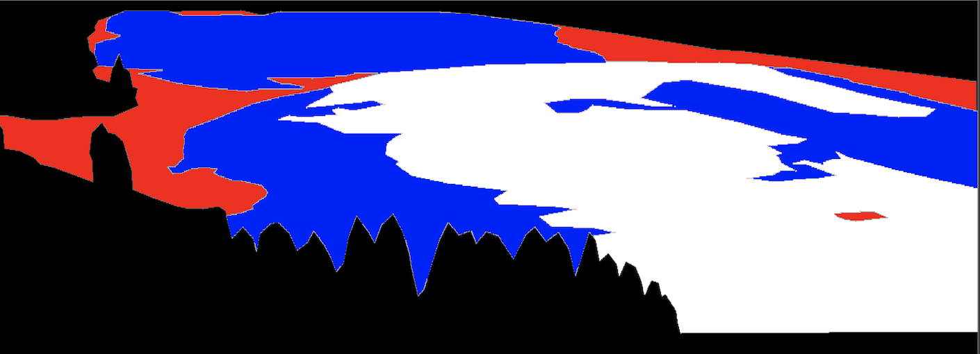
(d) Ground truth

(e) Colour code.

Figure 1: (a) Example webcam image of lake St. Moritz, from the Photi-LakeIce dataset, (b) lake detection result, (c) lake ice segmentation result, (d) corresponding ground truth labels and (e) the colour code used throughout the paper.

To evaluate any model’s ability to generalise, and in particular to work with high-capacity deep learning methods, one requires a large and diverse pool of annotated data, i.e., images with pixel-accurate labels. Webcams on lakes are a challenging outdoor scenario with limited image quality, and prone to unfavorable illumination, haze, etc; making it at times hard to distinguish between ice/snow or water, even for the human eye, see Fig. 2. For our study, we gathered and annotated several webcam streams. These include the data from four lakes and three summers for lake detection, and two lakes and two winters for lake ice segmentation. Entire data is curated and labelled by human annotators.

Contributions.

1. We set a new state of the art for lake ice detection from webcam data.

2. Unlike prior art (Tom et al.,, 2019), our method generalises well across different cameras and lakes, and across different winters.

3. Along the way we also demonstrate automated lake detection; a small extension that, however, may be very useful when scaling to many lakes or moving to non-stationary (pan-tilt-zoom) cameras.

4. We introduce Deep-U-Lab which produces visibly more accurate segment boundaries.

5. We report, for the first time, lake ice detection results for crowd-sourced images from image-sharing websites.

6. We make available a new Photi-LakeIce dataset of webcam images, with ground truth annotations for multiple lakes and winters.

(a) water

(b) water

(c) water + ice

(d) ice

(e) snow + ice

(f) snow

Figure 2: Texture variability of water, ice, and snow in the Photi-LakeIce dataset.

2 RELATED WORK

Lake ice monitoring. To our knowledge, Xiao et al., (2018) proposed lake ice detection with webcams for the first time. The authors used the FC-DenseNet model (Jégou et al.,, 2016) and performed experiments on a single lake (St. Moritz) for the winter $2016$-$17$. Another work was reported on monitoring lake ice and freezing trends from low-resolution optical satellite data (Tom et al.,, 2018). They used support vector machines to detect ice and snow on four Alpine lakes in Switzerland (Sihl, Sils, Silvaplana, and St. Moritz). Building on those works, an integrated monitoring system combining satellite imagery, webcams and in-situ data was proposed in Tom et al., (2019). Note that this work reported results on two winters ($2016$-$17$ and $2017$-$18$) for the webcam at lake St. Moritz. Duguay, Wang, and Wang (2019) provided algorithms to generate a bedfast/floating lake ice product from Synthetic Aperture Radar (SAR), and Wang et al., (2018) investigated the performance of a semi-automated segmentation algorithm for lake ice classification using dual-polarized RADARSAT-2 imagery. Du et al., (2019) summarised the physical principles and methods in remote sensing of selected key variables related to ice, snow, permafrost, water bodies, and vegetation.

The starting point for the present work was the observation that the work of Tom et al., (2019) failed to generalise across different cameras viewing the same lake. Our goal was to make progress towards a system that can be applied not only to different views of the same lake, but also to other lakes and/or data from different winters. As an even more extreme test, we also test on crowd-sourced data.

Amateur images for environmental monitoring. Besides lake ice, there are many more domains where images from webcams or photo-sharing repositories could benefit environmental monitoring. Examples include Li et al., (2017); Thorpe et al., (2011); Hoonhout et al., (2015); Wang et al., (2017); Surdu et al., (2015); Norouzzadeh et al., (2018); Alberton et al., (2017); Bothmann et al., (2017). Perhaps the closest ones to our work are, on the one hand, Salvatori et al., (2011), where the goal was to detect the extent of snow cover in webcam images; and on the other hand, Singh et al., (2019), where different types of floating ice on rivers were detected with the help of UAV images. We note that crowd-sourcing techniques are, in general, becoming more popular for environmental monitoring, e.g., Giuliani et al., (2016).

Deeplab v3+ for semantic segmentation. Due to their unmatched versatility and empirical performance, neural networks have become the preferred tool for many complex image analysis tasks, and remote sensing is no exception. For the task of semantic segmentation, Deeplab v3+ (Chen et al.,, 2018) is one of the most popular architectures, and the top performer on several different datasets; including generic consumer pictures, e.g., PASCAL VOC (Everingham et al.,, 2015), but also more specific ones like the recent ModaNet (Zheng et al.,, 2018), a large collection of street fashion images. Also in medical image analysis, Deeplab v3+ has been used to segment clinical image data, e.g., lesions of the liver in abdominal CT images (Xia et al.,, 2019). Remote sensing examples include detection of oil spills in satellite images (Krestenitis et al.,, 2019) to combat illegal discharges and tank cleaning that pollute the oceans. And, closer to our work, detecting different types of ice in UAV images (Singh et al.,, 2019) as an intermediate step to quantify river ice concentration with relatively small (in deep learning terms) datasets.

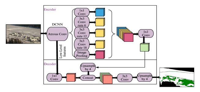
Figure 3: Deeplab v3+ architecture. Best if viewed on screen.

3 Methodology

3.1 Deeplab v3+

Deeplab v3+ (Chen et al.,, 2018) is a CNN architecture for semantic segmentation, designed to learn multi-scale contextual features while controlling signal decimation, see Fig. 3. The basic structure is a classical encoder-decoder architecture. We use Xception65 as the encoder backbone, which is similar to the well-known Inception network (Szegedy et al.,, 2015), except that it uses depth-wise separable convolutions. That is, 2D convolutions are applied on each input channel independently, then combined with 1D convolutions across channels. This saves a lot of unknowns, without any noticeable performance penalty. Moreover, all max-pooling operations are replaced by (depth-wise separable) strided convolutions.

Specific to Deeplab v3+ is the use of Atrous Spatial Pyramid Pooling (ASPP), to mitigate spatial smoothing but still encode multi-scale context. Atrous convolution dilates the kernel by an integer dilation rate $k$, such that only every $k$-th pixel of the input layer is used, thus increasing the receptive field without downsampling the original input. Overall, the encoder has an output stride (spatial downsampling from input to final feature encoding) of $16$. In the decoder module, the encoded features are first upsampled by a factor of $4$, then concatenated with the low-level features from the corresponding encoder layer (after reducing the dimensionality of the latter via $1\times 1$ convolution). These resulting “mid-resolution” features are transformed with a further stage of $3\times 3$ convolutions, then upsampled again by a factor $4$ to recover an output map at the full input resolution.

Deep-U-Lab. To mitigate the model’s tendency towards overly smooth, imprecise segment boundaries, we add three extra skip connections from the entry and middle blocks of the encoder, in the spirit of U-net (Ronneberger et al.,, 2015). We call this new version Deep-U-Lab, see Fig. 4. The corresponding feature maps are directly concatenated together with the final output of the encoder block. We found that they help to better preserve high-frequency detail at segment boundaries. The main task of the encoder is to extract high-level features for various classes, with a tendency to loose low-level information not crucial for that task. Hence, we enforce preservation of low-level features through concatenation, so as to refine the class boundaries.

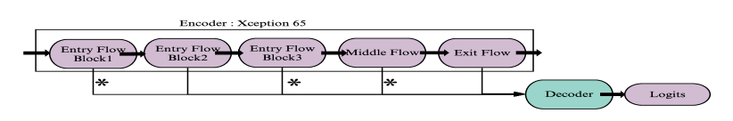
Figure 4: Deep-U-Lab. The newly added skip connections are marked by "*". Best if viewed on screen.

Transfer learning. A remarkable property of deep machine learning models is their ability to learn features that transfer well across datasets. We therefore initialise our training with network weights pre-trained on PASCAL VOC 2012 (Everingham et al.,, 2015), a standardised image dataset for basic objects like animals, people, vehicles, etc.. Even if there seemingly is a considerable domain shift between an existing image collection (in our case PASCAL) and a new dataset (our lake ice images), starting from a network learnt for the older dataset and fine-tuning it quickly adapts it to the new data and task, with much less data. In particular, batch normalization layers for a large network are difficult to train, because it calls for big batch sizes and thus GPU memory. Transfer learning comes to rescue in scenarios like this.

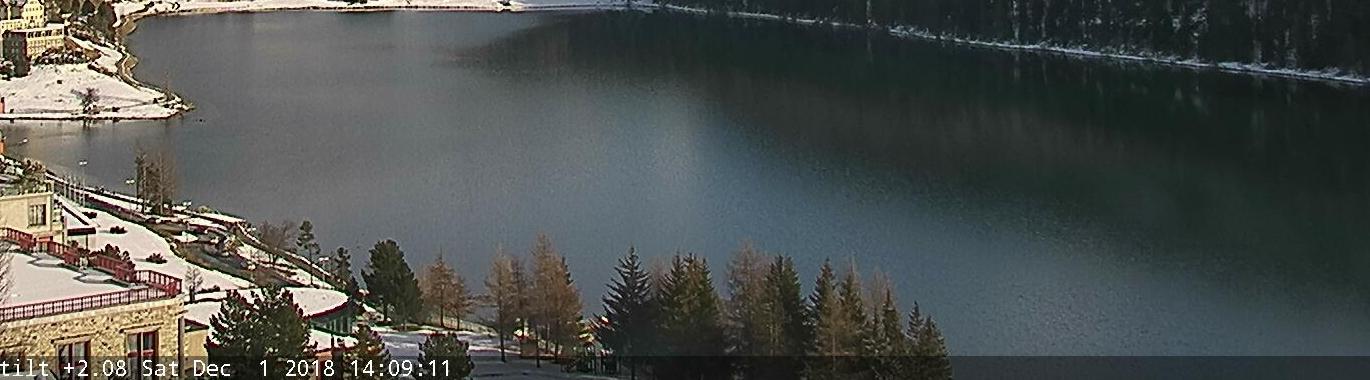
(a) Cam0 St. Moritz

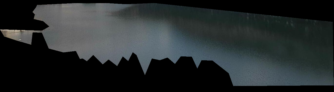
(b) Cam0 St. Moritz FG

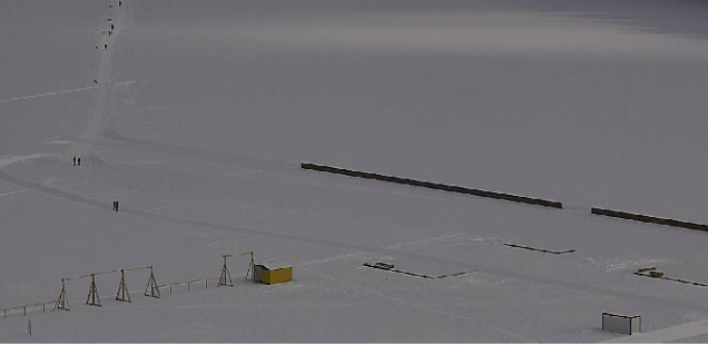
(c) Cam1 St. Moritz

(d) Cam1 St. Moritz FG

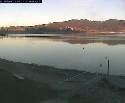
(e) Cam2 Sihl (R1)

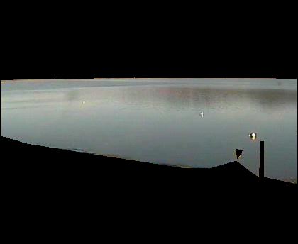
(f) Cam2 Sihl (R1) FG

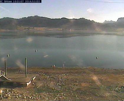
(g) Cam2 Sihl (R2)

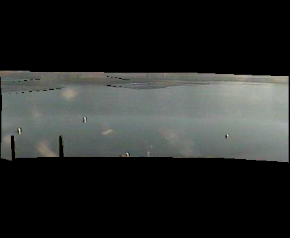
(h) Cam2 Sihl (R2) FG

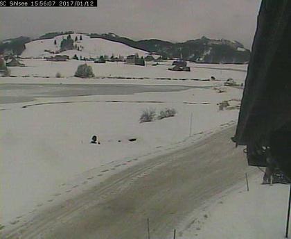
(i) Cam2 Sihl (R3)

(j) Cam2 Sihl (R3) FG

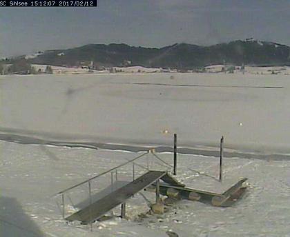
(k) Cam2 Sihl (R4)

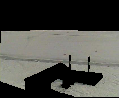
(l) Cam2 Sihl (R4) FG

Figure 5: Example images from the Photi-LakeIce dataset. 1${}^{\text{st}}$ row: fixed cameras monitoring lake St. Moritz. 2${}^{\text{nd}}$ and 3${}^{\text{rd}}$ rows: rotating camera (R1, R2, R3, R4 represents different rotations) monitoring lake Sihl. Even columns show the foreground (FG) lake area for the images shown in the previous column.

3.2 Lake detection

It is obvious that classifying lake ice is a lot easier if restricted to pixels on the lake. Full webcam frames usually include a lot of background (buildings, mountains, sky, etc.), and passing them directly to the lake ice classifier can add unnecessary distractions to the learning and inference stages (e.g., clouds can be difficult to discriminate from snow). Therefore, we prefer to localise the lake in a pre-processing step and run the actual lake ice detection only on lake pixels. For static webcams, it is relatively easy to localise the lake manually, as in earlier works  (Xiao et al.,, 2018; Tom et al.,, 2019). There are, however, situations where an automatic procedure would be preferable, for instance, if the lake level varies greatly over the years. Automatic detection of the lake becomes vital if also crowd-sourced images have to be analysed, since these are typically taken from variable, unknown viewpoints.

In the context of our work, it is natural to also cast the automatic lake detection as a two-class (foreground, background) pixel-wise semantic segmentation problem and train another instance of the segmentation model. For static webcams, we run the lake detector on summer images, to sidestep the situation where both the lake and the surrounding ground is covered with snow.

3.3 Lake ice segmentation

Once the lake mask has been determined, the state of the lake is inferred with a fine-grained classifier. In this step, pixels are labelled as one of four classes (water, ice, snow, clutter). From the per-pixel maps, we also extract two parameters often used to describe the temporal dynamics of the freezing cycle: the ice-on date, defined as the first day on which the large majority of the lake surface is frozen, and which is followed by a second day with also mostly frozen lake  (Franssen, Scherrer, and Scherrer, 2008); and the ice-off date, defined symmetrically as the first day on which a non-negligible part of the lake surface is liquid water, and followed by a second non-frozen day.

4 Data

4.1 Webcam data

All our webcam images are manually annotated with the LabelMe tool (Wada,, 2016) to generate pixel-wise ground truth. Additionally, the dataset is cleaned by discarding excessively noisy images due to bad weather (thick fog, heavy rain, and extreme illumination conditions). The images vary in spatial resolution, magnification, and tilt, depending on camera type (fixed or rotating) and parameters.

Lake detection dataset. For the task of lake detection, we have collected image streams from four different lakes: one camera each for lakes Sihl (rotating), Sils (fixed), and St. Moritz (rotating) and four cameras (all fixed) for lake Silvaplana. Refer to Table 2 for more details.

Winter	Lake	Cam	#images	Res
2016-17	St. Moritz	Cam0	820	324$\times$1209
2016-17	St. Moritz	Cam1	1180	324$\times$1209
2016-17	Sihl	Cam2	500	344$\times$420
2017-18	St. Moritz	Cam0	474	324$\times$1209
2017-18	St. Moritz	Cam1	443	324$\times$1209
2017-18	Sihl	Cam2	600	344$\times$420

Table 1: Key figures of the Photi-LakeIce dataset for different winters, lakes, and cameras.

Photi-LakeIce dataset. We report lake ice segmentation results on the Photi-LakeIce dataset, which we make publicly available to the research community. The dataset comprises of images from two lakes (St. Moritz, Sihl) and two winters (W$2016$-$17$ and W$2017$-$18$). See Table 1 for details. For images in this dataset, we also provide pixel-wise ground truth for foreground-background segmentation as well as for lake ice segmentation. There are two different, fixed webcams (Cam0 and Cam1, see Fig. 5a and c) both observing lake St. Moritz at different zoom levels. The third camera (Cam 2), at lake Sihl, rotates around one axis and observes the lake in four different viewing directions. Example images are shown in Fig. 5. Additionally, Fig. 6 shows the class frequencies for all classes (background + 4 states on the lake), which are fairly imbalanced with ice and clutter always being under-represented. For lake Sihl, there are four different camera angles involved in capturing distinct lake views, causing the difference in background frequencies. The background frequencies of the same camera slightly vary across different winters (such as Cam0 of St. Moritz) mostly due to differences in manual annotations, as these two winters are annotated by two different operators.

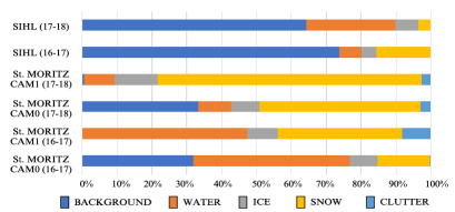
Figure 6: Class imbalance (ground-truth) in the Photi-LakeIce dataset. Best if viewed on-screen.

4.2 Crowd-sourced data

As an even more extreme generalisation task than between different webcam views, we also test the method on individual images sourced from online image-sharing platforms. We note that there is a potential to also include such images as complementary data sources in a monitoring system, as long as they are time-stamped. We employed keywords such as frozen St. Moritz, lake ice St. Moritz, St. Moritz lake in winter etc. to gather lake ice images from online platforms such as Google, Flickr, Pinterest, etc. In total, we collected $150$ images, which are all resized to a spatial resolution of $512\times 512$ for further use. Examples are shown in Figs. 13a and 14a.

5 EXPERIMENTS, RESULTS and DISCUSSION

Network details All networks are implemented in Tensorflow. The lake detection model is trained on image crops of size $500\times 500$, whereas the lake ice segmentation model, is trained with crop of size $321\times 321$. The evaluation of the (fully convolutional) networks is always run at full image resolution without any cropping. The per-class losses are balanced by re-weighting the cross-entropy loss with the inverse (relative) frequencies in the training set. All models are trained for $100$ epochs with batch sizes of $4$ for lake detection and $8$ for lake ice segmentation, respectively. Atrous rates are set to [$6,12,18$] in all experiments. Simple stochastic gradient descent empirically worked better than more sophisticated optimisation techniques. The base learning rate is set to $10^{-5}$ and reduced according to the poly schedule (Liu et al.,, 2015).

5.1 Results on webcam images

Train set		Test set		mIoU
Lakes	#images	Lake	#images
Silv, Moritz, Sihl	7477	Sils	2075	0.93
Silv, Sils, Sihl	8456	Moritz	1096	0.92
Silv, Sils, Moritz	9104	Sihl	448	0.93
Silv(0,1,2), SMS	7652	Silv(3)	1900	0.95
Silv(0,1,3), SMS	7906	Silv(2)	1646	0.95
Silv(0,2,3), SMS	8676	Silv(1)	876	0.90
Silv(1,2,3), SMS	8041	Silv(0)	1511	0.94

Table 2: Mean IoU (mIoU) values of the leave-one-cam-out experiments for lake detection. Silv(0,1,2,3) are the different camera angles for lake Silvaplana. SMS refers to {Sils, St. Moritz, Sihl}.

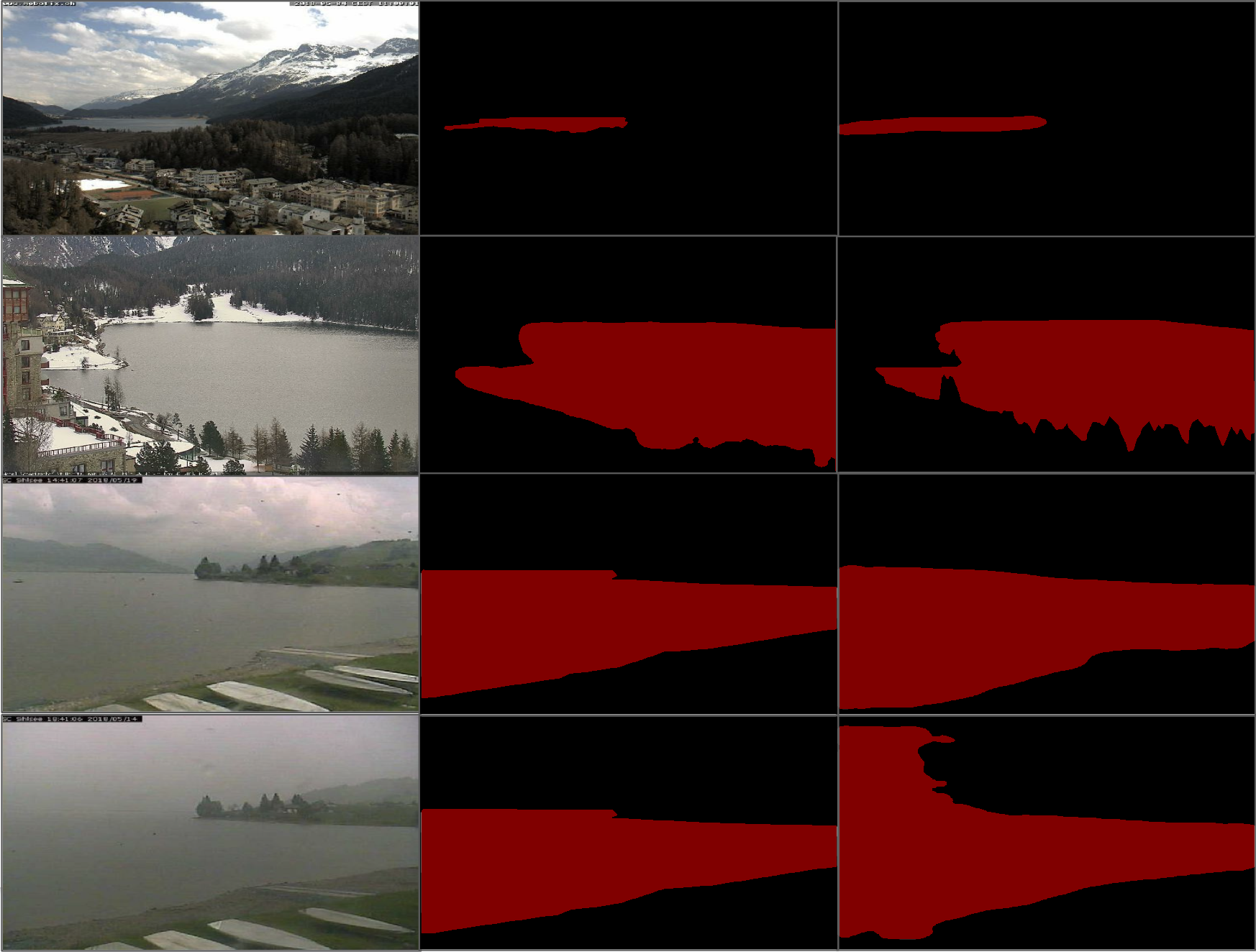
(a) Image

(b) Ground truth

(c) Prediction

Figure 7: Results of lake detection using Deeplab v3+. The first three rows shows successful cases, a failure case is displayed in the last row.

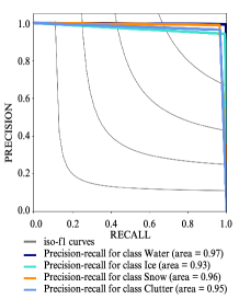
(a) Cam0 (test) results when trained using the data from Cam0 (train).

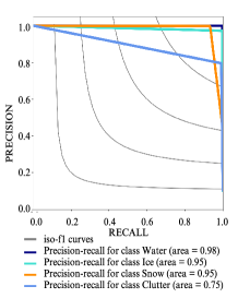
(b) Cam1 (test) results when trained using the data from Cam1 (train).

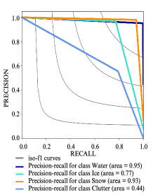
(c) Cam0 results when trained using the data from Cam1.

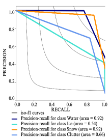
(d) Cam1 results when trained using the data from Cam0.

Figure 8: Precision-recall curves (Lake St. Moritz). Best if viewed on screen.

(a) Webcam image

(b) Ground truth

(c) Deep-U-Lab

(d) Deeplab v3+

Figure 9: Deeplab v3+ vs. Deep-U-lab. Segmentation boundaries are visibly crisper and more accurate with additional skip connections.

Lake	Train set		Test set		Water	Ice	Snow	Clutter	mIoU
	Cam	Winter	Cam	Winter
St. Moritz	Cam0	16-17	Cam0	16-17	0.98 / 0.70	0.95 / 0.87	0.95 / 0.89	0.97 / 0.63	0.96 / 0.77
St. Moritz	Cam1	16-17	Cam1	16-17	0.99 / 0.90	0.96 / 0.92	0.95 / 0.94	0.79 / 0.62	0.92 / 0.85
St. Moritz	Cam0	17-18	Cam0	17-18	0.97	0.88	0.96	0.87	0.93
St. Moritz	Cam1	17-18	Cam1	17-18	0.93	0.84	0.92	0.84	0.89
Sihl	Cam2	16-17	Cam2	16-17	0.79	0.62	0.81	—	0.74
Sihl	Cam2	17-18	Cam2	17-18	0.81	0.69	0.86	—	0.79
St. Moritz	Cam0	16-17	Cam1	16-17	0.76 / 0.36	0.75 / 0.57	0.84 / 0.37	0.61 / 0.27	0.74 / 0.39
St. Moritz	Cam1	16-17	Cam0	16-17	0.94 / 0.32	0.75 / 0.41	0.92 / 0.33	0.48 / 0.43	0.77 / 0.37
St. Moritz	Cam0	17-18	Cam1	17-18	0.62	0.66	0.89	0.42	0.64
St. Moritz	Cam1	17-18	Cam0	17-18	0.59	0.67	0.91	0.51	0.67
St. Moritz	Cam0	16-17	Cam0	17-18	0.64 / 0.45	0.58 / 0.44	0.87 / 0.83	0.59 / 0.40	0.67 / 0.53
St. Moritz	Cam0	17-18	Cam0	16-17	0.98	0.91	0.94	0.58	0.87
St. Moritz	Cam1	16-17	Cam1	17-18	0.86 / 0.80	0.71 / 0.58	0.93 / 0.92	0.57 / 0.33	0.77 / 0.57
St. Moritz	Cam1	17-18	Cam1	16-17	0.93	0.76	0.86	0.65	0.80
Sihl	Cam2	16-17	Cam2	17-18	0.61	0.14	0.35	—	0.51
Sihl	Cam2	17-18	Cam2	16-17	0.41	0.18	0.45	—	0.50

Table 3: Lake ice segmentation results (IoU) on the Photi-LakeIce dataset. For comparison, we also show results of Tom et al., (2019) where available, in grey. We outperform them in all instances.

Lake detection results. Only summer images are used to avoid problems due to snow cover (on both the lake and the surroundings). The model performed well with $\geq$0.9 mean Intersection-over-Union (mIoU) score (weighted according to the class distribution in the train set) in all cases, see Table 2. We are not aware of any previous work on lake detection in webcam images, but note that water bodies are in general segmented rather well in RGB images. Figure 7 shows the qualitative results of the lake detection, including a failure case in the last row. It can be observed that the wrong classification occurs in a rather foggy image that is difficult to judge even for humans. Also, note the fairly good prediction in the first row, a challenging case where the lake covers $<$5% of the image.

Lake ice segmentation results.

Table 3 shows the results for lake ice segmentation on the Photi-LakeIce dataset. Exhaustive experiments were performed to evaluate same camera train-test (rows 1-6), cross-camera train-test (rows 7-10) and cross-winter train-test (rows 11-16).

For the same camera train-test experiments, the model is trained randomly on $75\%$ of the images and tested on the remaining $25\%$. As shown in Table 3 (rows 1 and 2), the mIoU scores of the proposed approach are respectively $19$ and $7$ percent points higher than the ones reported by Tom et al., (2019). For lake St. Moritz, in addition to the results on the winter $2016$-$17$, we report results for the winter $2017$-$18$. Additionally, we present results on a second, more challenging lake (Sihl), for both winters. As can be seen in Fig. 5, the images from lake Sihl (Cam2) are of significantly lower quality, with severe compression artifacts, low spatial resolution, and small lake area in pixels, which amplifies the influence of small, miss-classified regions on the error metrics. Consequently, our method performs worse than for St. Moritz, but still reaches $>$76% correct classification under the rather strict IoU metric. We note that there is no clutter class since no events take place on lake Sihl.

The main drawback of prior studies on lake ice detection is their models’ inability to generalise from one camera view to another (Xiao et al.,, 2018; Tom et al.,, 2019). For the cross-camera experiments (rows 7-10, Table 3), our model is trained on all images from one camera and tested on all images from another camera. As per Table 3, for winter $2016$-$17$, the mIoU results for that experiment surpass the FC-DenseNet (Tom et al.,, 2019) by margin of $35$ to $40$ percent points. This huge improvement clearly shows the superior ability of the deep learning architecture to learn generally applicable “visual concepts” and avoid overfitting to specific sensor characteristics and viewpoints. For completeness, we also report cross camera results for winter $2017$-$18$. They are a bit worse than those for $2016$-$17$, due to more complex appearance and lighting during that season (e.g., black ice) that cause increased confusion between ice and water.

For an operational system, the ultimate goal is to train on the data from a set of lakes from one, or a few, winters and then apply the system in further winters, without the need to annotate further reference data. Hence, we also performed cross-winter experiments to assess the generalisation across winters. i.e., the model is trained on the data from one full winter and tested on the data acquired from the same viewpoint over a second winter. The results (Table 3, rows 11-16) show that the model also generalises quite well across winters. For St. Moritz, a model trained on winter $2016$-$17$ reaches an IoU of $77$% on $2017$-$18$, a gain of 20 percent points over prior art (Tom et al.,, 2019). For Cam0, there is also a substantial gain of $14$ percent points. It can, however, also be seen that there is still room for improvement in less favorable imaging settings such as lake Sihl, where the segmentation of ice and snow in a different winter largely fails.

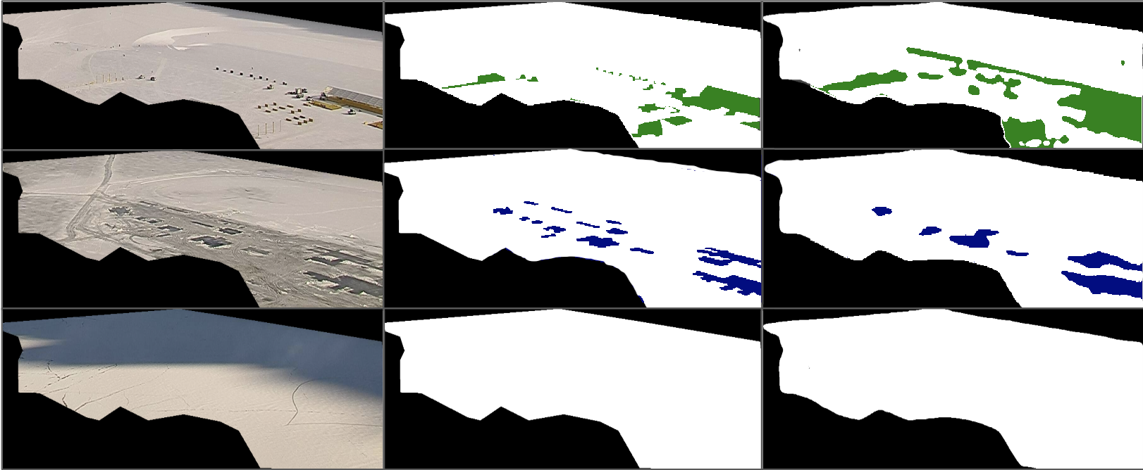
(a) Image

(b) Ground Truth

(c) Prediction

Figure 10: Cam0 results when the model is trained only on Cam1.

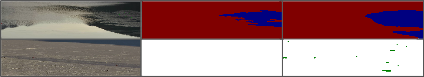
(a) Image

(b) Ground Truth

(c) Prediction

Figure 11: Cam1 results when the model is trained only on Cam0.

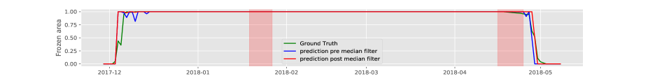
Figure 12: Frozen area time series with- and without post-processing: results of Cam0 when the network is trained using the data from Cam1. Red bars indicate periods of data gaps, where no images are stored due to technical failures.

For a more comprehensive assessment of the per-class results we also generate precision-recall curves, see Fig. 8. It can be seen that the performance for ice and clutter is inferior to the other two classes. A large part of the errors for clutter are actually due to imprecise ground truth rather than prediction errors of the model, as the annotated masks for thin and intricate structures like flagpoles, food stalls and individual people on the lake tend to be “bulk annotations” that greatly inflate the (relative) amount of clutter in the ground truth, leading to large (relative) errors. According to the curves, thresholds of 0.60 precision and 0.80 recall shows good a trade-off between the true-positive and false-positive rates for cross-camera results. However for same-camera results, the thresholds are much better ranging from 0.80 for Cam1 to 0.90 for Cam0.

Qualitative example results are shown in Figs. 10 and 11. Sometimes the images are even confusing for humans to annotate correctly, e.g., Fig. 10, row 2 shows an example of ice with smudged snow on top, for which the “correct” labeling is not well-defined. We note that our segmentation method is robust against cloud/mountain shadows cast on the lake (row 3). In another interesting case (Fig. 11, row 2) the network “corrects” human labeling errors, where humans are present on the frozen lake, but not annotated due to their small size.

Ice-on/off results. Freeze-up and break-up periods are of particular interest for climate monitoring.

Lake	Winter	Ice-on	Ice-off
St. Moritz	16-17	14.12.16	18.03-26.04.17
St. Moritz	17-18	06.12.17	27.04.18
Sihl	16-17	29.12.16,	31.12.17,
		04.01.17,	05.01.17,
		07.01.17,	11.01.17,
		10.02.17	14.02.17
Sihl	17-18	29.12.17,	02.01.18,
		15.02.18,	23.03.18,
		27.03.18,	05.04.18,
		11.04.18	16.04.18

Table 4: Ice-on/off dates predicted by our approach.

To estimate the ice-on/off dates, we produce a daily time series of the (fractional) frozen lake area in a camera’s field of view, for the winter $2017-18$ (Figs. 12). The areas in individual images are aggregated with a daily median, then smoothed with another 3-day median. The latter filters out individual days with difficult conditions and improves the model predictions by almost $3\%$. The estimated ice-on/off dates are shown in Table 4. We determined the ice-on/off dates for lake St. Moritz from Cam0, which covers a larger portion of the lake. For lake Sihl, multiple ice-on and off dates are found, as that lake is in a warmer (lower) region of Switzerland and froze/thawed four times within the same winter. See Table 4.

Water	Ice	Snow	Clutter	mIoU
0.60	0.32	0.71	0.79	0.60

Table 5: Lake ice segmentation results (IoU) on crowd-sourced dataset.

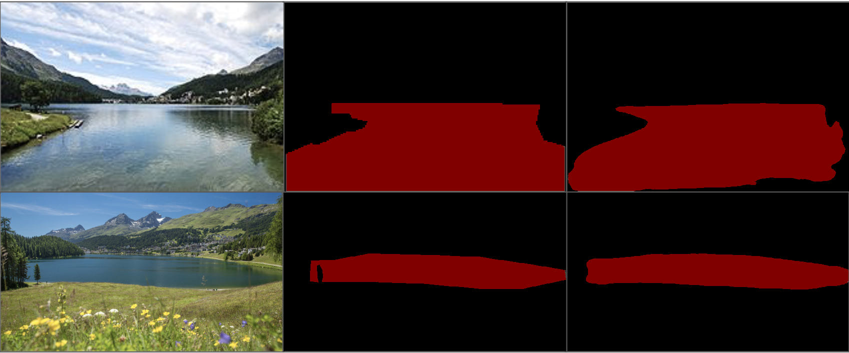
(a) Image

(b) Ground truth

(c) Prediction

Figure 13: Lake detection on crowd-sourced data.

5.2 Results on crowd-sourced images

Crowd-sourced images have a rather different data distribution, among others due to better image sensors and optical components, less aggressive compression, more vivid colours due to on-device electronics and image editing, etc. Thus, they are, arguably, an even more challenging test of model generalisation. With the model trained on webcam images (St. Moritz winter $2016$-$17$), lake detection in crowd-sourced images yields an IoU of 75% for the background and 64% for the lake. Qualitative results are shown in Fig. 13.

For the semantic segmentation task, we apply the model trained on webcam images (St. Moritz winter $2016$-$17$) on the crowd-sourced images. Quantitative results are presented in Table 5. Note that these are still significantly better than the cross-camera generalisation results of Tom et al., (2019). Qualitative examples are shown in Fig. 14.

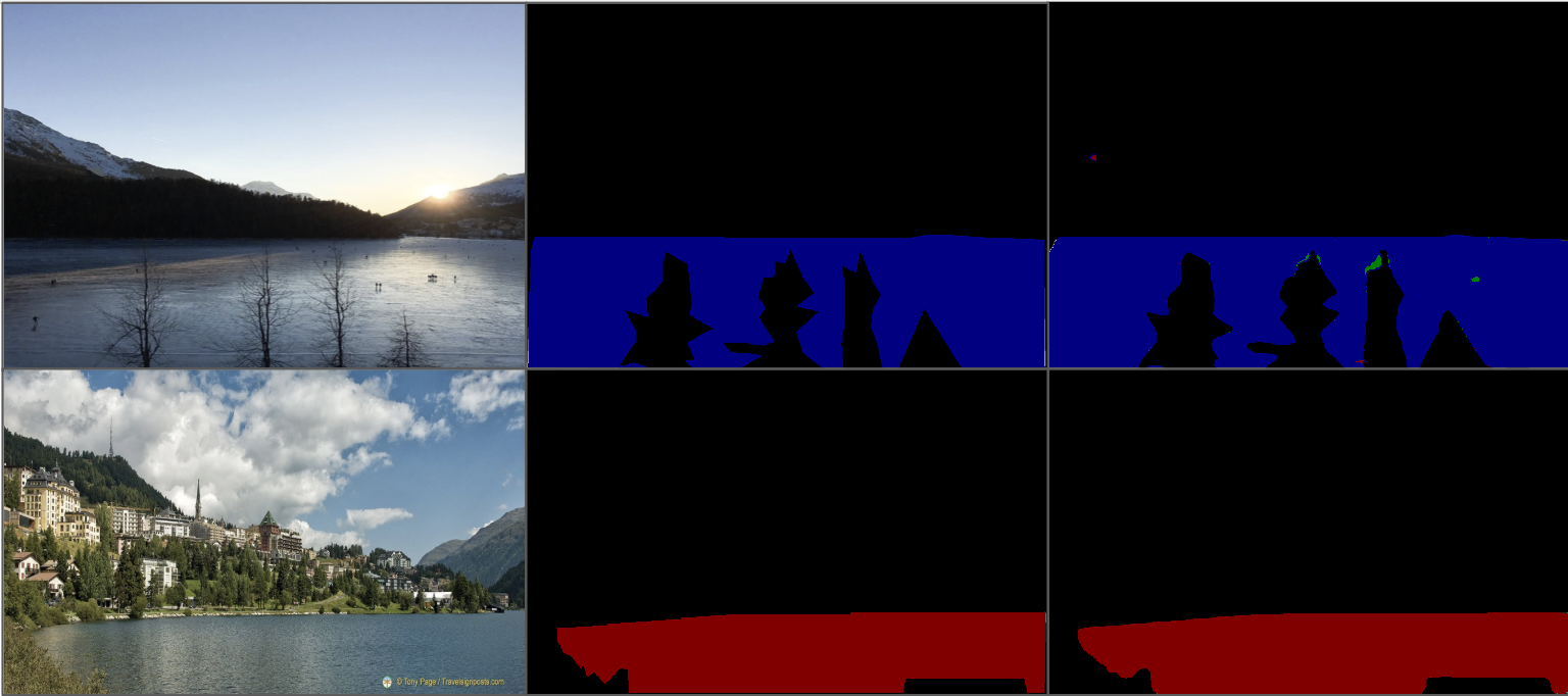
(a) Image

(b) Ground truth

(c) Prediction

Figure 14: Lake ice segmentation on crowd-sourced data.

5.3 Discussion

A natural question that arises is: Why does Deep-U-Lab perform a lot better compared to FC-DenseNet for lake ice detection? While it is difficult to conclusively attribute the empirical performance of deep neural networks to specific architectural choices, we speculate that there are two main reasons why Deep-U-Lab is superior to FC-DenseNet.

First, by following a popular “standard” architecture, we can start from very well pre-trained weights – yet another confirmation that the benefits of pre-training on big datasets often outweigh the perceived domain gap to specific sensor and application settings. Unfortunately, we could not complete the comparison by training Deep-U-Lab from scratch with our data, as this did not converge. Second, our model has a much larger receptive field around every pixel, due to the atrous convolutions. It appears that long-range context and texture, which only our model can exploit, play an important role for lake ice detection.

6 CONCLUSION AND OUTLOOK

One conclusion that we drew from our study is that the previous, pioneering attempts (Xiao et al.,, 2018; Tom et al.,, 2019) underestimated the potential of deep convolutional networks for lake ice detection with webcams. We found that with modern high-performance architectures like Deeplab v3+, in particular our variant Deep-U-lab, segmentation results are near-perfect within the data of one camera over one winter (i.e., in the scenario where a portion of the data is annotated manually, then extrapolation to the remaining frames is automatic). Moreover, also generalisation to different views of the same lake, as well as to different winters with the same camera viewpoint, works fairly well. Especially the latter case is very interesting for an operational scenario: it is quite likely that a system trained on data from two or three winters would reach well above 80% IoU for all classes of interest. Moreover, it appears within reach to even complement dedicated monitoring cameras (or, in touristic places, public webcams) with amateur images opportunistically gleaned from the web.

An open question for future work is how to minimise the initial annotation effort, to simplify the introduction of monitoring systems especially at new locations. A fascinating extension could be to adopt ideas from few-shot learning and/or active learning to quickly adapt the system to new locations.

References

- Alberton et al., (2017) Alberton, B., da S. Torres, R., Cancian, L. F., Borges, B. D., Almeida, J., Mariano, G. C., dos Santos, J., Morellato, L. P. C., 2017. Introducing digital cameras to monitor plant phenology in the Tropics: Applications for conservation. Perspectives in Ecology and Conservation, 15(2).
- Bothmann et al., (2017) Bothmann, L., Menzel, A., Menze, B. H., Schunk, C., Kauermann, G., 2017. Automated processing of webcam images for phenological classification. Plos One, 12(2).
- Chen et al., (2018) Chen, L.-C., Zhu, Y., Papandreou, G., Schroff, F., Adam, H., 2018. Encoder-decoder with atrous separable convolution for semantic image segmentation. European Conference on Computer Vision (ECCV).
- Cordts et al., (2016) Cordts, M., Omran, M., Ramos, S., Rehfeld, T., Enzweiler, M., Benenson, R., Franke, U., Roth, S., Schiele, B., 2016. The Cityscapes dataset for semantic urban scene understanding. Computer Vision and Pattern Recognition (CVPR).
- Du et al., (2019) Du, J., Watts, J. D., Jiang, L., Lu, H., Cheng, X., Duguay, C., Farina, M., Qiu, Y., Kim, Y., Kimball, J. S., Tarolli, P., 2019. Remote sensing of environmental changes in cold regions: methods, achievements and challenges. Remote Sensing, 11(16).
- Duguay, Wang, (2019) Duguay, C., Wang, J., 2019. Advancement in bedfast lake ice mapping from Sentinel-1 SAR data. International Geoscience and Remote Sensing Symposium (IGARSS).
- Everingham et al., (2015) Everingham, M., Eslami, S. M. A., Van Gool, L., Williams, C. K. I., Winn, J., Zisserman, A., 2015. The Pascal visual object classes challenge: A retrospective. International Journal of Computer Vision, 111(1).
- Franssen, Scherrer, (2008) Franssen, H. J. H., Scherrer, S. C., 2008. Freezing of lakes on the Swiss plateau in the period 1901–2006. International Journal of Climatology, 28(4).
- Giuliani et al., (2016) Giuliani, M., Castelletti, A., Fedorov, R., Fraternali, P., 2016. Using crowdsourced web content for informing water systems operations in snow-dominated catchments. Hydrology and Earth System Sciences, 20(12).
- Hoonhout et al., (2015) Hoonhout, B., Radermacher, M., Baart, F., Maaten, L., 2015. An automated method for semantic classification of regions in coastal images. Coastal Engineering, 105.
- Jégou et al., (2016) Jégou, S., Drozdzal, M., Vázquez, D., Romero, A., Bengio, Y., 2016. The one hundred layers Tiramisu: Fully convolutional DenseNets for semantic segmentation. Computer Vision and Pattern Recognition Workshops (CVPRW).
- Krestenitis et al., (2019) Krestenitis, M., Orfanidis, G., Ioannidis, K., Avgerinakis, K., Vrochidis, S., Kompatsiaris, I., 2019. Oil spill identification from satellite images using deep neural networks. Remote Sensing, 11(15).
- Li et al., (2017) Li, S., Fu, H., Lo, W.-L., 2017. Meteorological visibility evaluation on webcam weather image using deep learning features. International Journal of Computer Theory and Engineering, 9(6).
- Liu et al., (2015) Liu, W., Rabinovich, A., Berg, A. C., 2015. ParseNet: Looking wider to see better. arXiv preprint, arXiv:1506.04579.
- Norouzzadeh et al., (2018) Norouzzadeh, M. S., Nguyen, A., Kosmala, M., Swanson, A., Palmer, M. S., Packer, C., Clune, J., 2018. Automatically identifying, counting, and describing wild animals in camera-trap images with deep learning. Proceedings of the National Academy of Sciences, 115(25).
- Ronneberger et al., (2015) Ronneberger, O., Fischer, P., Brox, T., 2015. U-Net: Convolutional networks for biomedical image segmentation. Medical Image Computing and Computer-assisted Intervention (MICCAI).
- Salvatori et al., (2011) Salvatori, R., Plini, P., Giusto, M., Valt, M., Salzano, R., Montagnoli, M., Cagnati, A., Crepaz, G., Sigismondi, D., 2011. Snow cover monitoring with images from digital camera systems. Italian Journal of Remote Sensing, 43(2).
- Singh et al., (2019) Singh, A., Kalke, H., Ray, N., Loewen, M., 2019. River ice segmentation with deep learning. arXiv preprint, arXiv:1901.04412.
- Surdu et al., (2015) Surdu, C. M., Duguay, C. R., Pour, H. K., Brown, L. C., 2015. Ice freeze-up and break-up detection of shallow lakes in Northern Alaska with spaceborne SAR. Remote Sensing, 7(5).
- Szegedy et al., (2015) Szegedy, C., Liu, W., Jia, Y., Sermanet, P., Reed, S. E., Anguelov, D., Erhan, D., Vanhoucke, V., Rabinovich, A., 2015. Going deeper with convolutions. Computer Vision and Pattern Recognition (CVPR).
- Thorpe et al., (2011) Thorpe, A., Roberts, D., Dennison, P., Bradley, E., Funk, C., 2011. Detection of trace gas emissions from point sources using shortwave infrared imaging spectrometry. AGU Fall Meeting Abstracts.
- Tom et al., (2018) Tom, M., Kälin, U., Sütterlin, M., Baltsavias, E., Schindler, K., 2018. Lake ice detection in low-resolution optical satellite images. ISPRS Annals of Photogrammetry, Remote Sensing and Spatial Information Sciences, IV-2.
- Tom et al., (2019) Tom, M., Suetterlin, M., Bouffard, D., Rothermel, M., Wunderle, S., Baltsavias, E., 2019. Integrated monitoring of ice in selected Swiss lakes. Final Project Report.
- Wada, (2016) Wada, K., 2016. LabelMe: Image polygonal annotation with Python. https://github.com/wkentaro/labelme.
- Wang et al., (2018) Wang, J., Duguay, C. R., Clausi, D. A., Pinard, V., Howell, S. E. L., 2018. Semi-automated classification of lake ice cover using dual polarization RADARSAT-2 imagery. Remote Sensing, 10(11).
- Wang et al., (2017) Wang, L., Scott, K. A., Clausi, D. A., 2017. Sea ice concentration estimation during freeze-up from SAR imagery using a convolutional neural network. Remote Sensing, 9(5).
- Xia et al., (2019) Xia, K., Yin, H., Qian, P., Jiang, Y., Wang, S., 2019. Liver semantic segmentation algorithm based on improved deep adversarial networks in combination of weighted loss function on abdominal CT images. IEEE Access, 7.
- Xiao et al., (2018) Xiao, M., Rothermel, M., Tom, M., Galliani, S., Baltsavias, E., Schindler, K., 2018. Lake ice monitoring with webcams. ISPRS Annals of Photogrammetry, Remote Sensing and Spatial Information Sciences, IV-2.
- Zheng et al., (2018) Zheng, S., Yang, F., Kiapour, M. H., Piramuthu, R., 2018. ModaNet: A large-scale street fashion dataset with polygon annotations. ACM Multimedia.