Grid-based minimization at scale: Feldman-Cousins corrections for SBN

Abstract.

We present a computational model for the construction of Feldman-Cousins (FC) (Feldman and Cousins, 1998) corrections frequently used in High Energy Physics (HEP) analysis. The program contains a grid-based minimization and is written in C++. Our algorithms exploit vectorization through Eigen3 (Guennebaud et al., 2010), yielding a single-core speed-up of 350 compared to the original implementation, and achieve MPI data parallelism by using DIY (Morozov and Peterka, 2016). We demonstrate the application to scale very well at High Performance Computing (HPC) sites. We use HDF5 (The HDF Group, NNNN) in conjunction with HighFive (The Blue Brain Project, NNNN) to write results of the calculation to file.

Conventions

In this work, mathematical vectors are denoted as lower-case bold variables. Similarly, we use upper-case bold variables to denote matrices. We are using the Cori machines at the National Energy Research Scientific Computing Center (NERSC) (National Energy Research Scientific Computing Center, [n.d.]), and refer to them and their chips as Cori phase 1 (Haswell) or Cori phase 2 (KNL). (See Table 1 for details.)

Machine	Cori phase 1 (Haswell)	Cori phase 2 (KNL)
CPU	Intel Xeon E5-2698 v3	Intel Xeon Phi 7250
Clockspeed	2.3 GHz	1.4 GHz
Cores per node	32	68

Table 1. Processors used in this work.

1. Introduction

The Short Baseline Neutrino (SBN) experimental program (Antonello et al., 2015), comprising three Liquid Argon Time Projection Chamber (LArTPC) neutrino detectors, is about to begin operations at Fermi National Accelerator Laboratory, in order to study neutrino interactions from a dedicated accelerator-based neutrino beam with unprecedented precision. The experiment will measure and compare neutrino interaction rates recorded by each detector to precisely test theories involving new particle states, and typically involving a large number of theoretical model parameters. Efforts are ongoing to determine the “sensitivity” of the SBN experimental program to theoretical models, and further optimize it in terms of a number of SBN experimental design parameters. Such sensitivity studies can be performed using the Feldman-Cousins prescription (Feldman and Cousins, 1998). This prescription provides a method for producing sensitivity contours in a multi-dimensional parameter space (corrected frequentist confidence intervals) through fits accounting for, generally, non-gaussian systematic uncertainties. The F.C. prescription is computationally expensive and is typically implemented using multi-universe techniques. One study run will typically use O(10M) CPU hours depending on the dimensionality of the problem and the desired resolution. The SBN collaboration employs the F.C. analysis procedure as part of their analysis frameworks, including a framework known as SBNfit (Cianci et al., 2017). This paper provides a summary of the work we have completed in adapting this SBNfit framework to run efficiently on HPC facilities. This effort is particularly crucial for SBN, where some of the theories that SBN aims to definitively test involve models with up to $D=12$ independent fit parameters.

The task at hand is to perform a parameter scan in a $D$-dimensional parameter space to find regions that are compatible with a central data vector $\mathbf{c}$ of length $N$, which represents the experimentally observed data. Each point $\mathbf{p}$ is associated with a vector of length $N$, representing $N$ predicted observations; we refer to this vector as signal or $\mathcal{S}(\mathbf{p})$. The goal of the scan is to build, through repeated fits to “fake experimental data,” a distribution of a statistical measure ($\Delta\chi^{2}$) for each $\mathbf{p}$, which effectively describes the number of degrees of freedom in the fit in the vicinity of that point. The effective number of degrees of freedom subsequently determine associated critical values for the statistical measure used to quantify compatibility of any given $\mathbf{p}$ from a fit performed to “real experimental data”.

The procedure to build the distribution of $\Delta\chi^{2}$ is performed using a multi-universe approach, where, in each universe, the input data is fluctuated around its mean following established techniques. The number of universes to simulate is a program parameter that we will refer to as $N_{\text{univ}}$. An example distribution of $\Delta\chi^{2}$ along with an illustration of critical values can be found in Fig. 1.

At the heart of the computation is the calculation of a quantity called $\chi^{2}$. The inputs are two vectors $\mathbf{a}$ and $\mathbf{b}$ of size $N$ and a symmetric, positive definite matrix, $\mathbf{M}$, of size $N\times N$, representing the inverese of a “covariance matrix.” The covariance matrix encapsulates systematic and statistical uncertainties on the prediction vector. The $\chi^{2}$ measure allows for a statistical interpretation of the numerical similarity of $\mathbf{a}$ and $\mathbf{b}$ taking into account uncertainties and correlations encoded in $\mathbf{M}$:

(1) $$\chi^{2}=(\mathbf{a}-\mathbf{b})^{\top}\cdot\mathbf{M}\cdot(\mathbf{a}-\mathbf{b})$$

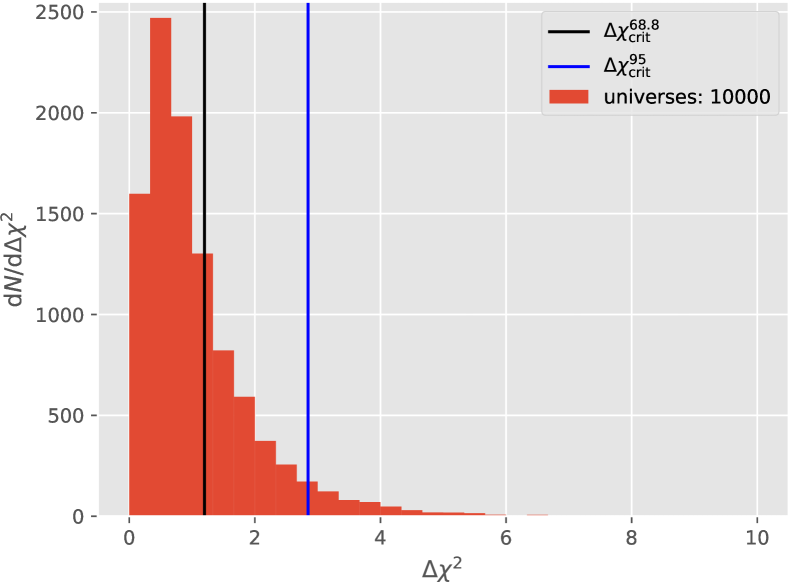
Figure 1. An example $\Delta\chi^{2}$ distribution for a single $\mathbf{p}$ obtained from 10,000 universes. The vertical lines indicate the critical values of $\Delta\chi^{2}$, left of which lie 68.8% and 95% of the distribution, as indicated on the legend.

The paper is organized as follows: in Section 2 we introduce the algorithm used for the computation of the Feldman-Cousins correction. We follow in Section 3 with detailed discussions of challenges and solutions to achieve computational performance and scalability. The achieved performance and eventual limitations are explained in Section 4. We make our concluding remarks in Section 5 and discuss prospects of future development.

2. Algorithm

The computational approach chosen for the parameter scan is to first discretize the parameter space by means of a rigid rectangular grid, which is then linearized to take on the form of a list ($\mathcal{G}$) of the points in the $D$-dimensional grid. We will refer to the length of $\mathcal{G}$ as $N_{\text{gridpoints}}$.

To build the distribution $\Delta\chi^{2}$ for a single point $\mathbf{p}\in\mathcal{G}$, a total of $N_{\text{univ}}$ calculations, comparing a given (fluctuated) prediction at $\mathbf{p}$ with first-principles-predictions at all other $N_{\text{gridpoints}}$ points, are performed. Algorithm 1 shows a pseudo-code representation of the most relevant steps. For a single universe and following the notation in (1), the procedure is as follows:

1. Calculate signal prediction $\mathcal{S}(\mathbf{p})$

2. Fluctuate $\mathcal{S}(\mathbf{p})$, yielding $\mathbf{d}$

3. For each point $\mathbf{q}\in\mathcal{G}$: calculate $\chi^{2}(\mathbf{d},\mathcal{S}(\mathbf{q}),\mathbf{M})$

4. Determine $\mathbf{q}_{\text{min}}$ for which $\chi^{2}$ is minimal

5. Update $\mathbf{M}$ for $\mathbf{q}_{\text{min}}$ and repeat scan over $\mathbf{q}$ until $\chi^{2}_{\text{min}}$ convergence is reached at some new $\mathbf{q}_{\text{min}}$

6. Return $\Delta\chi^{2}=\chi^{2}(\mathbf{d},\mathbf{c},\mathbf{M})-\chi^{2}(\mathbf{d},\mathcal{S}(\mathbf{q}_{\text{min}}),\mathbf{M})$

where $\mathbf{c}$ is the central prediction (experimentally measured data). This means that the computational complexity, and therefore the program run time, can be expected to scale $\propto N_{\text{univ}}\cdot N_{\text{gridpoint}}^{2}$. Measurements of the scaling are given in more detail in Section 4. An example distribution of $\Delta\chi^{2}$ along with an illustration of critical values can be found in Fig. 1. This procedure follows the fit methodology of (Aguilar-Arevalo et al., 2013) as a typical HEP implementation of the F.C. correction.

Algorithm 1 Building the $\Delta\chi^{2}$ distribution for a single $\mathbf{p}\in\mathcal{G}$ and a central prediction vector $\mathbf{c}$. In principle there can be an additional loop around lines 7 to 14 aimed at updating the matrix $\mathbf{M}$. We chose to omit this here for clarity.

1:function buildDeltaChi2($\mathbf{p},\mathbf{c},\mathbf{M},\mathcal{S},N_{\text{univ}}$)

2:     $\mathbf{s}=\mathcal{S(\mathbf{p})}$ $\triangleright$ prediction at $\mathbf{p}$

3:     for $i\in[0,N_{\text{univ}})$ do

4:         $\chi^{2}_{\text{min}}\leftarrow\inf$;

5:         $\mathbf{p}_{\text{min}}=\mathbf{p}$

6:         $\mathbf{a}=$ fluctuation of $\mathbf{s}$

7:         for $\mathbf{q}\in\mathcal{G}$ do $\triangleright$ Iterate over all grid points

8:              $\mathbf{b}=\mathcal{S(\mathbf{q})}$

9:              chi2=calcChi2$(\mathbf{a},\mathbf{b},\mathbf{M})$ $\triangleright$ using Algorithm 2

10:              if chi2 $<\chi^{2}_{\text{min}}$ then

11:                  $\chi^{2}_{\text{min}}\leftarrow$ chi2;

12:                  $\mathbf{p}_{\text{min}}=\mathbf{q}$

13:              end if

14:         end for

15:         deltaChi2 = calcChi2$(\mathbf{a},\mathbf{c},\mathbf{M})$ - $\chi^{2}_{\text{min}}$

16:     end for

17:The deltaChi2 values are aggregated and written to disk.

18:end function

Algorithm 2 $\chi^{2}$ calculation

1:function calcChi2($\mathbf{a},\mathbf{b},\mathbf{M}$)

2:     $\mathbf{d}\leftarrow\mathbf{a}-\mathbf{b}$

3:     $\chi^{2}=\mathbf{d}^{\top}\cdot\mathbf{M}\cdot\mathbf{d}$

4:     return $\chi^{2}$

5:end function

3. Computational challenges and solutions

Listing 1: Implementation of (1) using Eigen3

⬇

double calcChi(VectorXd const & a,

VectorXd const & b,

MatrixXd const & M )

{

auto const & diff = a-b;

return diff.transpose() * M * diff;

}

Listing 2: Original implementation of (1)

⬇

double calcChi(vector<double> a,

vector<double> b,

vector<vector< double> > M,

int N)

{

double chi2 = 0;

for(int i =0; i<N; i++){

for(int j =0; j<N; j++){

chi2 += (a[i]-b[i]) * M[i][j] * (a[j]-b[j] );

}

}

return chi2;

}

The calculation of $\Delta\chi^{2}$ at a single $p\in\mathcal{G}$ requires the knowledge of the signal $\mathcal{S}(\mathbf{p})$ for all $\mathbf{p}\in\mathcal{G}$. In the original implementation the calculation of $\mathcal{S}(\mathbf{p})$ was computationally expensive due to the code not being vectorized, frequent access of the file-system and the coming and going of objects. This is why the original implementation resorted to precomputing and caching $\mathcal{S}(\mathbf{p})$ — ultimately leading to severe limitations on the problem size due to memory exhaustion. The re-implementation, which is heavily based on Eigen3, solves all these issues and completely offsets the performance gain from caching meaning that the limitation on the size of problem that can be solved is solely due to the available compute time.

The computational complexity of the program is dependent on two factors. One being the number of multiverses, $N_{\text{univ}}$, that are simulated. We find the computational cost to be linearly dependent on $N_{\text{univ}}$. The other factor being the number of points, $N_{\text{gridpoints}}$ in the grid, which the run time depends on quadratically.

Algorithm 3 Original implementation of computation of $\mathcal{S}(\mathbf{p})$

1:procedure signal($\mathbf{p}$) $\triangleright$ comment

2:     Determine which files to open for $\mathbf{p}$

3:     Open 2 ROOT files and read TH1D objects into two vector¡TH1D¿

4:     Select physics parameters based on $\mathbf{p}$

5:     Call T1HD::Scale on elements of vector¡TH1D¿ in a nested for-loop

6:     Compute a vector¡double¿ from the vector¡TH1D¿

7:     Add this vector¡double¿ to another vector¡double¿

8:     Return that vector¡double¿

9:end procedure

The major obstacle for an MPI-parallel version of the code that scales well on an HPC system was the frequent access of the file system in the original implementation. The same data was read from file any time objects were created. This put an undue burden on the file system, ultimately leading to poor performance and scaling. The solution was to read any of the input files only once during the program life-time and to use collective MPI operations to copy data to all ranks trough memory. In the original implementation, each calculation of the $\mathcal{S}(\mathbf{p})$ required the opening of two ROOT files and the traversal and manipulation of the objects therein, which is very expensive. Given that the $\mathcal{S}(\mathbf{p})$ need to known for all $\mathbf{p}\in\mathcal{G}$ to compute the desired quantities, a caching of the $\mathcal{S}(\mathbf{p})$ was present in the original implementation. Albeit improving the performance of the program significantly, this approach ultimately lead to a restriction on the problem size that could be tackled as the amount of memory needed grows with $N_{\text{gridpoints}}$, ultimately exhausting the system memory.

Further, the coming and going of ROOT objects, such as TH1D histograms, turned out to be a major performance bottleneck. These ROOT histogram objects have many mathematical operations associated with them. Performance issues were eliminated by substituting these histograms objects with data types and operations from Eigen3. The histogram methods turned out to be a non-optimal choice for necessary mathematical manipulations in this program, as the bulk of the computations are matrix-vector multiplications and array operations. Eigen3’s VectorXd and MatrixXd are simply much better suited for these operations, as they inherently make use of the vectorisation and thus grant a significant performance benefit — so much so that the original gain from caching the computations of the $\mathcal{S}(\mathbf{p})$ in memory could completely be offset. A comparison of signal prediction rates is shown in Table 2. These changes effectively transform the program from one limited by available memory into a one limited only by CPU.

	Frequency of $\mathcal{S}(\mathbf{p})$
Original, Haswell	30 Hz
New, Haswell	10 MHz
New, KNL	2 MHz

Table 2. Comparison of single-core signal prediction rates. The achieved speed-up allows to avoid having to cache $\mathcal{S}(\mathbf{p})$ and thus eliminate the memory-limitation of the problem size.

A further important change was the use of HDF5 as output file format. We are using the MPI-capable file objects for writing to disk which reduces necessary MPI communications to a minimum. This is especially suitable for the problem at hand as the information written do disk is comprised of trivial data types. Further, the amount of data written by every rank as well as their target location within the HDF5 datasets is is completely deterministic and thus known upon start of the program.

The final revised application utilizes DIY(Morozov and Peterka, 2016) for data parallelism across processes and nodes, and Eigen3 for linear algebra and vectorized calculations. The application is now parameterized on number of universes, the number of grid points, and the standard MPI option for number of ranks.

4. Performance and scaling

In this section we measure the overall program execution time as a function of $N_{\text{univ}}$ and $N_{\text{gridpoint}}$ to test our initial hypothesis that the run time should scale $\propto N_{\text{univ}}\cdot N_{\text{gridpoint}}^{2}$. We further demonstrate strong scaling of the application and make an attempt at predicting the maximum size problem that can be solved when running on all of NERSC’s Cori for a full day.

4.1. Scaling with $N_{\text{univ}}$ and $N_{\text{gridpoint}}$

To collect the data, we used a fixed number of Haswell nodes (and therefore ranks) and varied $N_{\text{univ}}$ and $N_{\text{gridpoint}}$ independently. Fig. 2 show the scaling of the program time for a fixed number $N_{\text{gridpoint}}$ as a function of $N_{\text{univ}}$. The data is overlayed with a linear fit and there is no visible deviation from a linear scaling.

Similarly, in Fig. 3 we fix the number of universes and measure the program execution time as function of $N_{\text{gridpoint}}$. The quadratic fit to the data again shows no visible deviation from the expected behavior.

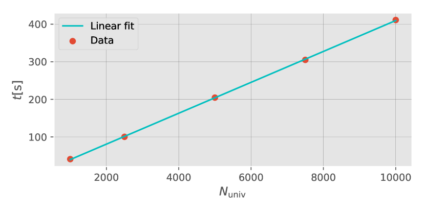
Figure 2. Scaling of the program run time with the number of universes, demonstrating a linear dependence on $N_{\text{univ}}$.

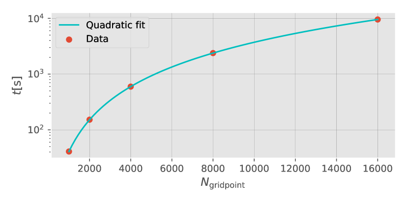
Figure 3. Scaling of the program run time with the number of grid points, demonstrating a quadratic dependence on $N_{\text{gridpoint}}$.

4.2. Single node scaling

We measure the program execution time as a function of the number of ranks in order to see in how far the program benefits from using multiple MPI ranks. Haswell nodes allow to run on up to two ranks per core, leading to a maximum of 64 ranks per node. On the KNL nodes it is possible to utilize up to four hardware threads per processor, resulting in a maximum number of ranks of 272 per node (See also Table 1).

We select a fixed size problem, distribute the work among the ranks as evenly as possible, and record the time spent in the main part of the program for each rank separately. For this application, the work is number of points from the parameter space and number of universes to generate. The data is shown in Fig. 4 for Haswell nodes and in Fig. 5 for KNL. The most relevant quantity in terms of throughput is of course the amount of time the slowest rank spends ($t_{\text{max}}$). For Haswell nodes we find the best performance when using 32 ranks, meaning our program does not benefit from threading. We also find that when using e.g. 33 or 34 ranks, i.e. effectively oversubscribing 1 and 2 cores respectively, the performance in terms of the total run time drops almost by a factor of two. The effect can be seen in Fig. 4. When utilizing 33 ranks, we are in a situation where two ranks are competing for resources on the same core. Similarly, when running with 34 ranks, we observe 4 ranks that are slower than the rest since they are visibly competing with each other. We repeat the measurements on a KNL node and find a similar picture. Again, using non-integer multiples of the number of cores (68) leads to an overall worse performance due to ranks competing for resources in an unbalanced way. In contrast to Haswell, however, we observe a gain in performance in terms of $t_{\text{max}}$ from using 2 and 4 ranks per core of 16% and 24% respectively.

Ranks	68	136	272
$t_{\text{max}}$[s]	87	75	70
Gain w.r.t. 68 ranks		16%	24%

Table 3. Total run time of a fixed problem on a single KNL node demonstrating that there is a mild benefit in using hardware threading.

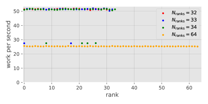
Figure 4. Measurement of the single Haswell node performance for a fixed problem size. The work is distributed among ranks and we measure the utilization of each rank in terms of units of work per second. Non-integer multiples of the number of cores available leads to a significant performance loss. We do not observe a benefit from using 2 ranks per core.

Figure 5. Measurement of the single KNL node performance for a fixed problem size. The work is distributed among ranks and we measure the utilization of each rank in terms of units of work per second. Non-integer multiples of the number of cores available leads to a significant performance loss. We observe a mild benefit from using 2 and 4 ranks per core.

4.3. Multi node scaling

For any distributed computing program it is crucial to know whether using N times as many computing resources yields a program execution time that is N times faster. In order to study this, we define a reasonable large problem of a fixed size and measure the time it takes to complete the main part of the program as a function of the number of Haswell nodes used ($N_{\text{nodes}}$). Following the finding in the previous section, we use 32 ranks per node in this study.

We further define the program execution efficiency as

(2) $$\varepsilon=N_{\text{nodes}}\cdot\frac{t(N_{\text{nodes}})}{t(1)},$$

where $t(1)$ is the run time on a single.

Our measurements are shown in Fig. 6 and demonstrate that the program scales reasonably well. Eventually the amount of work to be done per rank becomes relatively small and the drop to about 80% efficiency at 32 nodes (1024 ranks) indicates that the compute time of individual tasks may not be completely uniform.

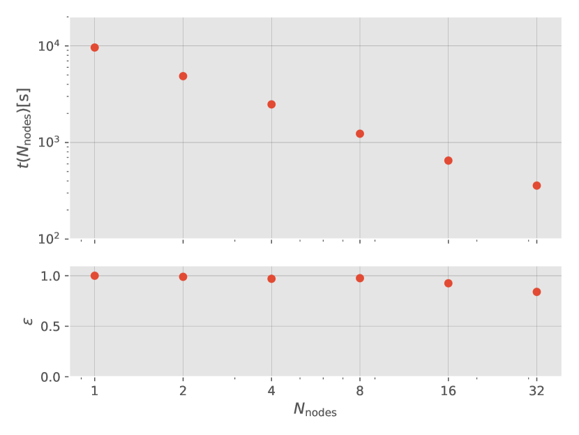
Figure 6. Strong scaling measurements on Haswell nodes. We observe generally good scaling up to the point where the amount of work per rank becomes relatively small.

4.4. Estimation of what is possible

In order to estimate the size of problem that can be tackled with a machine like Cori, we define the computation of $\mathcal{S(\mathbf{q})}$ and successive execution of calcChi (lines 8 and 9 of Algorithm 1) as core computation as it is a quantity that is independent of $N_{\text{gridpoint}}$ and $N_{\text{univ}}$. We then measure the numbers of core computations per second as a function of the number of nodes. We find the scaling to be linear in the number of nodes for our measurements. This allows to estimate an upper limit of of core computations if the whole machine were available. For Cori phase 1 (Haswell) we estimate an upper boundary of $6^{10}~{}s{-1}$ from a linear extrapolation to the entirety of 2388 nodes. Similarly, we find an upper boundary of $1.8^{11}~{}s{-1}$ when using all 9688 nodes of Cori phase 2 (KNL). The data and linear fits are shown in Fig. 7. It should be noted that the linear scaling assumption should be considered optimistic and be interpreted as an upper limit of the performance of the program.

We can use these numbers to estimate the size of, $\mathcal{G}$, that could possibly be solved with our implementation of the Feldman-Cousins method. A commonly occurring measure of statistical accuracy in that method is a significance level expressed in multiples of $\sigma$. For instance, $3\sigma$ and $5\sigma$ correspond to $N_{\text{univ}}=10^{4}$ and $N_{\text{univ}}=10^{8}$, respectively. In Table 4 we provide numbers of maximally possible grid sizes under the assumption of running on the entirety of Cori phase 1/2 for a full day. We find that for the $5\sigma$ significance level, which is typically applied to claim scientific discovery, only comparatively small problem sizes of about 10 thousand grid points can be solved. This translates into two-dimensional problems of fairly good resolution of 100 points per axis. In three dimensions, the resolution drops to about 20 points per axis. For higher dimensions the application of this method becomes computationally intractable.

	$N_{\text{univ}}=10^{4}$ ($3\sigma$)	$N_{\text{univ}}=10^{8}$ ($5\sigma$)
Cori phase 1 (Haswell)	$7.2\times 10^{5}$	$7.2\times 10^{3}$
Cori phase 2 (KNL)	$1.2\times 10^{6}$	$1.2\times 10^{4}$

Table 4. Upper boundaries on grid sizes that can be processed when running a full day on all of Cori phase 1/2.

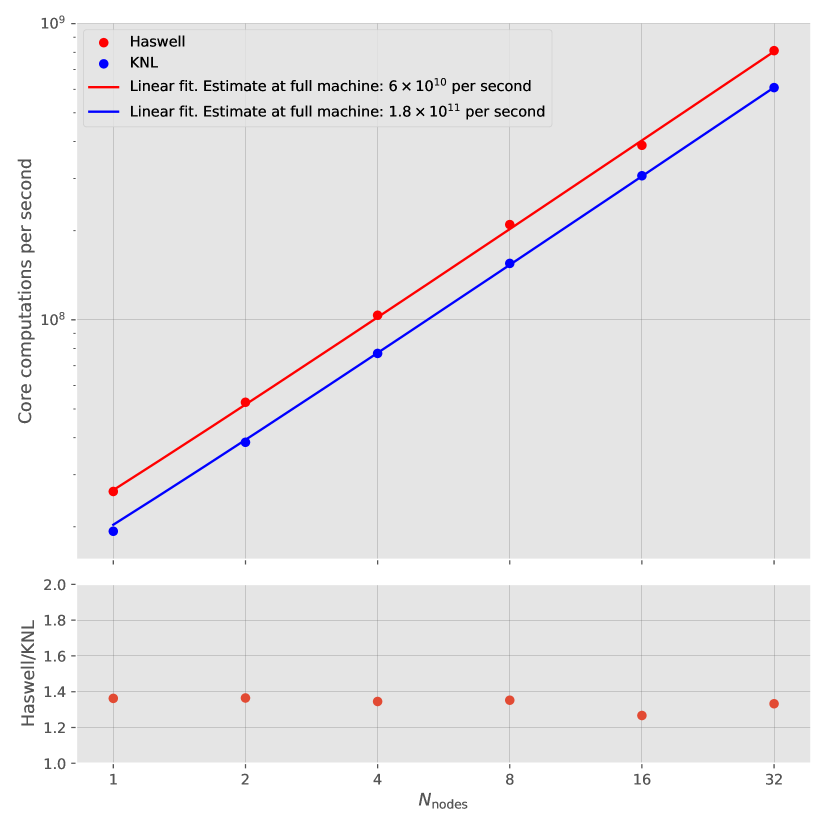
Figure 7. “Velocity” plot showing the “speed” of core computations on different architectures as function of the number of nodes.

5. Conclusions

The goal of this work has been to reconstruct the existing SBN application and algorithms that calculate Feldman-Cousins corrections to run efficiently on current state-of-the-art processor architectures and systems available at HPC facilities. We transformed a High Energy Physics problem common within neutrino physics from a serial-execution program limited by machine memory into an MPI-parallel application that scales up to available compute power of a facility. We obtain node-level and thread-level parallelism through DIY, and obtain significant performance improvements by restructuring algorithms to use Eigen3 for matrix multiplications and array manipulations.

An interesting side-effect of this work is the calculations performed within functions such as calcChi2 better represent the actual mathematical operations being performed on the data. Eigen provides a higher-level abstraction that greatly improves the readability of the code. This will allow for physics-developers to understand what is happening in this code if and when problems arise. It also provides better opportunities for the compiler and library to optimize the executable for specific platforms and architectures. This ought to be of great benefit to the experiment. Since the algorithms and procedures in this analysis application are so similar to experiments other than SBN, we believe the techniques employed here will provide similar benefits in terms of performance and design for the broader neutrino physics program.

5.1. Future work

For this round of improvements, we chose to stay with more traditional large-core libraries and techniques for vectorization within a compute node. Our next phase will explore changes necessary for evaluating the performance of GPU accelerators to further reduce the program execution time. For this future work, we will target Kokkos as a replacement for Eigen3.

We find that in spite of the achieved improvements, the computational complexity of the Feldman-Cousins approach coupled with SBN design choices for the current implementation severely limit the dimensionally of the problem that can be handled. The current “brute-force” method of scanning a regular grid becomes prohibitive after two or perhaps three dimensions. An alternative scanning approach will need to be found to move towards the seven or more dimensions that the experiment would like to probe, along with allowing $N_{\text{univ}}$ to be different for each $\mathbf{p}\in\mathcal{G}$, such that large numbers of universes are applied only in the vicinity of the eventual contour. We will be exploring alternative techniques to this grid scan through our connection with the SciDAC FASTmath Institute (FASTmath Institute, [n.d.]).

Incorporation of the new capabilities enabled by this work into the SBN experiment analysis workflow is underway. The reorganization of this application and efficient use of computational resources opens the door to incorporating more dimensions into the problem space that SBN aims to address. Replacement of the well-established and validated grid-scan procedure will require additional consideration and study within the SBN collaboration. Providing an alternative procedure and comparison study is part of our future work; the physics study and impact within SBN, however, falls outside of our scope. Nevertheless, our work ought to provide the machinery to greatly improve, for example, design parameters such as how much data will be necessary for the experiment to collect in order to achieve any given future physics goals.

- (1)
- Aguilar-Arevalo et al. (2013) A. A. Aguilar-Arevalo et al. 2013. Improved Search for Oscillations in the MiniBooNE Experiment. Phys. Rev. Lett. 110 (2013), 161801. https://doi.org/10.1103/PhysRevLett.110.161801 arXiv:hep-ex/1303.2588
- Antonello et al. (2015) M. Antonello et al. 2015. A Proposal for a Three Detector Short-Baseline Neutrino Oscillation Program in the Fermilab Booster Neutrino Beam. (2015). arXiv:physics.ins-det/1503.01520
- Cianci et al. (2017) Davio Cianci, Andy Furmanski, Georgia Karagiorgi, and Mark Ross-Lonergan. 2017. Prospects of Light Sterile Neutrino Oscillation and CP Violation Searches at the Fermilab Short Baseline Neutrino Facility. Phys. Rev. D96, 5 (2017), 055001. https://doi.org/10.1103/PhysRevD.96.055001 arXiv:hep-ph/1702.01758
- FASTmath Institute ([n.d.]) FASTmath Institute. [n.d.]. FASTmath is a program of the Office of Science within the Department of Energy. https://fastmath-scidac.llnl.gov/.
- Feldman and Cousins (1998) Gary J. Feldman and Robert D. Cousins. 1998. A Unified approach to the classical statistical analysis of small signals. Phys. Rev. D57 (1998), 3873–3889. https://doi.org/10.1103/PhysRevD.57.3873 arXiv:physics.data-an/physics/9711021
- Guennebaud et al. (2010) Gaël Guennebaud, Benoît Jacob, et al. 2010. Eigen v3. http://eigen.tuxfamily.org.
- Morozov and Peterka (2016) Dmitriy Morozov and Tom Peterka. 2016. Block-Parallel Data Analysis with DIY2. (2016). https://github.com/diatomic/diy.
- National Energy Research Scientific Computing Center ([n.d.]) National Energy Research Scientific Computing Center. [n.d.]. The Cori System at the NERSC. https://docs.nersc.gov/systems/cori/.
- The Blue Brain Project (NNNN) The Blue Brain Project. 2016-NNNN. HighFive. https://github.com/BlueBrain/HighFive.
- The HDF Group (NNNN) The HDF Group. 1997-NNNN. Hierarchical Data Format, version 5. http://www.hdfgroup.org/HDF5/.