LOGARITHMIC HÖLDER CONTINUOUS MAPPINGS AND BELTRAMI EQUATION

Abstract

The paper is devoted to the study of mappings satisfying the inverse Poletsky inequality. We study the local behavior of these mappings, moreover, we are most interested in the case when the corresponding majorant is integrable on some set of spheres of positive linear measure. The most important result is a logarithmic Hölder continuity of such mappings at inner points. As a corollary, we obtained the existence of a continuous $ACL$-solution of the Beltrami equation, which is logarithmic Hölder continuous.

2010 Mathematics Subject Classification: Primary 30C65; Secondary 31A15, 31B25

1 Introduction

As is known, mappings with bounded distortion satisfy the inequality

$$M(\Gamma)\leqslant N(f,A)\cdot K\cdot M(f(\Gamma))\,,$$ (1.1)

where $M$ is the modulus of families of paths $\Gamma$ in the domain $D,$

$$N(y,f,A)\,=\,{\rm card}\,\left\{x\in A:f(x)=y\right\}\,,\qquad N(f,A)\,=\,\sup\limits_{y\in{\mathbb{R}}^{n}}\,N(y,f,A)\,,$$

$A$ is a Borel set in $D,$ and $K\geqslant 1$ is some constant defined as

$$K={\rm ess\sup}\,K_{O}(x,f)\,.$$

Here we also used the common notation $K_{O}(x,f)=\|f^{\,\prime}(x)\|^{n}/J(x,f)$ for $J(x,f)\neq 0;$ $K_{O}(x,f)=1$ for $f^{\,\prime}(x)=0,$ and $K_{O}(x,f)=\infty$ for $f^{\,\prime}(x)\neq 0$ and $J(x,f)=0.$ In addition, regarding relation (1.1), we could point to the following papers, see e.g., [MRV₁, Theorem 3.2] or [Ri, Theorem 6.7.II]. Some similar condition applies to mappings whose have unbounded outher dilatations. In particular, the relation

$$M(\Gamma)\leq\int\limits_{f(E)}K_{I}\left(y,f^{\,-1},E\right)\cdot\rho_{*}^{n}(y)\,dm(y)\,,$$ (1.2)

holds for the so-called mappings with finite length distortion, where $E$ is an arbitrary measurable subset of $D,$ $\Gamma$ is a family of paths in $E$ and $\rho_{*}(y)\in{\rm adm\,}f(\Gamma)$ (see, e.g., [MRSY₂, Theorem 8.5]). In this manuscript, the main object of the study are mappings which satisfy some more general inequality than (1.2). More precisely, in relation (1.2), we will assume that there is a more abstract Lebesgue measurable function $Q,$ and all the problems related to Hölder continuity, which are studied in this article, we will try to connect with the behavior of this function. For estimates of Hölder type for many well-known classes of mappings, such as mappings with bounded distortion and quasiconformal mappings, see, e.g., [LV, Theorem 3.2.II], [Re, Theorem 1.1.2], [Va, Theorem 18.2, Remark 18.4], [MRV₁, Theorem 3.2] and [GG, Theorem 1.8]. Regarding the more general Hölder logarithmic continuity, we point out articles and monographs [Suv, Theorems 1.1.V and 2.1.V], [MRSY₂, Theorem 7.4], [MRSY₃, Theorem 3.1] and [RS, Theorem 5.11], cf. [Cr, Theorems 4 and 5]. We emphasize that, under some very special restrictions, such mappings are even Lipschitz, but this fact is very rare for mappings of such a general nature (see, e.g., [RSS₂, Theorem 1.1, Lemma 4.2, Theorem 4.1]).

In what follows, $M$ denotes the $n$-modulus of a family of paths, and the element $dm(x)$ corresponds to a Lebesgue measure in ${\mathbb{R}}^{n},$ $n\geqslant 2,$ see [Va]. For the sets $A,B\subset{\mathbb{R}}^{n}$ we set, as usual,

$${\rm diam}\,A=\sup\limits_{x,y\in A}|x-y|\,,\quad{\rm dist}\,(A,B)=\inf\limits_{x\in A,y\in B}|x-y|\,.$$

Sometimes, instead of ${\rm dist}\,(A,B),$ we also write $d(A,B),$ if a misunderstanding is impossible. Given sets $E$ and $F$ and a given domain $D$ in $\overline{{\mathbb{R}}^{n}}={\mathbb{R}}^{n}\cup\{\infty\},$ we denote by $\Gamma(E,F,D)$ the family of all paths $\gamma:[0,1]\rightarrow\overline{{\mathbb{R}}^{n}}$ joining $E$ and $F$ in $D,$ that is, $\gamma(0)\in E,$ $\gamma(1)\in F$ and $\gamma(t)\in D$ for all $t\in(0,1).$ Everywhere below, unless otherwise stated, the boundary and the closure of a set are understood in the sense of an extended Euclidean space $\overline{{\mathbb{R}}^{n}}.$ Let $x_{0}\in\overline{D},$ $x_{0}\neq\infty,$

$$B(x_{0},r)=\{x\in{\mathbb{R}}^{n}:|x-x_{0}|<r\}\,,\quad{\mathbb{B}}^{n}=B(0,1)\,,$$

$$S(x_{0},r)=\{x\,\in\,{\mathbb{R}}^{n}:|x-x_{0}|=r\}\,,S_{i}=S(x_{0},r_{i})\,,\quad i=1,2\,,$$

$$A=A(x_{0},r_{1},r_{2})=\{x\,\in\,{\mathbb{R}}^{n}:r_{1}<|x-x_{0}|<r_{2}\}\,.$$

Let $f:D\rightarrow{\mathbb{R}}^{n},$ $n\geqslant 2,$ and let $Q:{\mathbb{R}}^{n}\rightarrow[0,\infty]$ be a Lebesgue measurable function such that $Q(x)\equiv 0$ for $x\in{\mathbb{R}}^{n}\setminus f(D).$ Let $A=A(y_{0},r_{1},r_{2}).$ Let $\Gamma_{f}(y_{0},r_{1},r_{2})$ denotes the family of all paths $\gamma:[a,b]\rightarrow D$ such that $f(\gamma)\in\Gamma(S(y_{0},r_{1}),S(y_{0},r_{2}),A(y_{0},r_{1},r_{2})),$ i.e., $f(\gamma(a))\in S(y_{0},r_{1}),$ $f(\gamma(b))\in S(y_{0},r_{2}),$ and $\gamma(t)\in A(y_{0},r_{1},r_{2})$ for any $a<t<b.$ We say that $f$ satisfies the inverse Poletsky inequality at $y_{0}\in f(D)$ if the relation

$$M(\Gamma_{f}(y_{0},r_{1},r_{2}))\leqslant\int\limits_{A}Q(y)\cdot\eta^{n}(|y-y_{0}|)\,dm(y)$$ (1.3)

holds for any Lebesgue measurable function $\eta:(r_{1},r_{2})\rightarrow[0,\infty]$ such that

$$\int\limits_{r_{1}}^{r_{2}}\eta(r)\,dr\geqslant 1\,.$$ (1.4)

Note that the first author established the openness and discreteness of mappings in (1.3) under certain conditions on the function $Q,$ see, e.g., [Sev]. In a more general case, the performance of these properties is not guaranteed. Note also that the equicontinuity of homeomorphisms with condition (1.3) with somewhat less general constraints on the domain and the corresponding mappings is studied in detail in [SevSkv]. In this manuscript, we focus on mappings with branching.

We now formulate the main results of this article. To this end, we recall a few more definitions. A mapping $f:D\rightarrow{\mathbb{R}}^{n}$ is called a discrete if the preimage $\{f^{\,-1}(y)\}$ of each point $y\,\in\,{\mathbb{R}}^{n}$ consist of isolated points, and open if the image of any open set $U\subset D$ is an open set in ${\mathbb{R}}^{n}.$ In the extended Euclidean space $\overline{{{\mathbb{R}}}^{n}}={{\mathbb{R}}}^{n}\cup\{\infty\},$ we use the so-called chordal metric $h$ defined by the equalities

$$h(x,y)=\frac{|x-y|}{\sqrt{1+{|x|}^{2}}\sqrt{1+{|y|}^{2}}}\,,\quad x\neq\infty\neq y\,,\quad\,h(x,\infty)=\frac{1}{\sqrt{1+{|x|}^{2}}}\,.$$ (1.5)

For a given set $E\subset\overline{{\mathbb{R}}^{n}},$ we set

$$h(E):=\sup\limits_{x,y\in E}h(x,y)\,.$$ (1.6)

The quantity $h(E)$ in (1.6) is called the chordal diameter of the set $E.$

For given sets $A,B\subset\overline{{\mathbb{R}}^{n}},$ we put

$$h(A,B)=\inf\limits_{x\in A,y\in B}h(x,y)\,,$$

where $h$ is a chordal metric defined in (1.5).

For domains $D,D^{\,\prime}\subset{\mathbb{R}}^{n},$ $n\geqslant 2,$ and a Lebesgue measurable function $Q:{\mathbb{R}}^{n}\rightarrow[0,\infty]$ equal to zero outside the domain $D^{\,\prime},$ we define by $\mathfrak{R}_{Q}(D,D^{\,\prime})$ the family of all open discrete mappings $f:D\rightarrow D^{\,\prime}$ such that relation (1.3) holds for each point $y_{0}\in D^{\,\prime}.$

Theorem 1.1. Let $D$ and $D^{\,\prime}$ be domains in ${\mathbb{R}}^{n},$ $n\geqslant 2,$ and let $D^{\,\prime}$ be a bounded domain. Suppose that, for each point $y_{0}\in D^{\,\prime}$ and for every $0<r_{1}<r_{2}<r_{0}:=\sup\limits_{y\in D^{\,\prime}}|y-y_{0}|$ there is a set $E\subset[r_{1},r_{2}]$ of a positive linear Lebesgue measure such that the function $Q$ is integrable over the spheres $S(y_{0},r)$ for every $r\in E.$ Then the family of mappings $\mathfrak{R}_{Q}(D,D^{\,\prime})$ is equicontinuous at each point $x_{0}\in D.$

Theorem 1 generalizes the result of [SevSkv, Theorem 1.5] to the case when mappings may have branch points, and the corresponding function $Q$ may turn out to be non-integrable in the considered domain $D.$ In particular, Theorem 1 implies the following obvious

Corollary 1.1. Assume that under the conditions of Theorem 1

$$\int\limits_{S(y_{0},r)}Q(y)\,d\mathcal{H}^{n-1}(y)<~{}\infty$$

for almost all $r\in(0,r_{0})$ and any $y_{0}\in D^{\,\prime}.$ Then the family of mappings $\mathfrak{R}_{Q}(D,D^{\,\prime})$ is equicontinuous at each point $x_{0}\in D.$

For a domain $D\subset{\mathbb{R}}^{n},$ $n\geqslant 2,$ and a Lebesgue measurable function $Q:{\mathbb{R}}^{n}\rightarrow[0,\infty],$ we define by $\mathfrak{F}_{Q}(D)$ the family of all open discrete mappings $f:D\rightarrow{\mathbb{R}}^{n}$ such that relation (1.3) holds for each point $y_{0}\in f(D).$ In the case where the function $Q$ behaves somewhat better, and the domain $D$ is the unit ball, the following result holds. Note that the original (local) version of this result was published by us in [SSD, Theorem 1.1].

Theorem 1.2. Let $n\geqslant 2,$ and let $Q\in L^{1}({\mathbb{R}}^{n}).$ Suppose that $K$ is a compact set in ${\mathbb{B}}^{n}.$ Now, the inequality

$$|f(x)-f(y)|\leqslant\frac{C_{n}\cdot(\|Q\|_{1})^{1/n}}{\log^{1/n}\left(1+\frac{r_{0}}{2|x-y|}\right)}$$ (1.7)

holds for any $x,y\in K$ and $f\in\mathfrak{F}_{Q}({\mathbb{B}}^{n}),$ where $\|Q\|_{1}$ denotes $L^{1}$-norm of $Q$ in ${\mathbb{R}}^{n},$ $C_{n}>0$ is some constant depending only on $n,$ and $r_{0}=d(K,\partial{\mathbb{B}}^{n}).$

Remark 1.1. If the domain $D$ does not have finite boundary points, then we will consider the number $r_{0}$ to be any positive. The said agreement will apply to the entire subsequent text of the manuscript.

A separate case of Theorems 1 and 1, and also the Corollary 1, is a situation when $f$ is a homeomorphism in $D.$ In this case, let us denote $g:=f^{\,-1}$ and remark that

$$g(\Gamma(S(y_{0},r_{1}),S(y_{0},r_{2}),f(D)))=\Gamma_{f}(y_{0},r_{1},r_{2})\,.$$ (1.8)

In fact, if $\gamma\in g(\Gamma(S(y_{0},r_{1}),S(y_{0},r_{2}),f(D))),$ then $\gamma:[a,b]\rightarrow{\mathbb{R}}^{n},$ and $\gamma=g\circ\alpha,$ $\alpha:[a,b]\rightarrow{\mathbb{R}}^{n}$ and $\alpha(a)\in S(y_{0},r_{1}),$ $\alpha(b)\in S(y_{0},r_{2}),$ $\alpha(t)\in f(D)$ for $a\leqslant t\leqslant b.$ Now, $\gamma(t)\in D$ for $a\leqslant t\leqslant b$ and $f(\gamma)=\alpha\in\Gamma(S(y_{0},r_{1}),S(y_{0},r_{2}),f(D)),$ i.e., $\gamma\in\Gamma_{f}(y_{0},r_{1},r_{2}).$ Thus, $g(\Gamma(S(y_{0},r_{1}),S(y_{0},r_{2}),f(D)))\subset\Gamma_{f}(y_{0},r_{1},r_{2}).$ The inverse inclusion is proved similarly.

For domains $D,D^{\,\prime}\subset{\mathbb{R}}^{n},$ $n\geqslant 2,$ and a Lebesgue measurable function $Q:{\mathbb{R}}^{n}\rightarrow[0,\infty]$ equal to zero outside the domain $D,$ we define by $\mathfrak{R}^{*}_{Q}(D,D^{\,\prime})$ the family of all homeomorphisms $g$ of $D^{\,\prime}$ onto $D$ such that relation

$$M(f(\Gamma(S(x_{0},r_{1}),S(x_{0},r_{2}),D)))\leqslant\int\limits_{D}Q(x)\cdot\eta^{n}(|x-x_{0}|)\,dm(x)$$ (1.9)

holds for $f=g^{\,-1},$ each $x_{0}\in D,$ any $0<r_{1}<r_{2}<d_{0}=\sup\limits_{x\in D}|x-x_{0}|$ and any Lebesgue measurable function $\eta:(r_{1},r_{2})\rightarrow[0,\infty]$ with the condition (1.4). Taking into account Theorem 1, Theorem 1 and Corollary 1 and relation (1.8), we obtain the following statement.

Corollary 1.2. Let $D$ and $D^{\,\prime}$ be domains in ${\mathbb{R}}^{n},$ $n\geqslant 2,$ and let $D$ be a bounded domain. Suppose that $Q:{\mathbb{R}}^{n}\rightarrow[0,\infty]$ is a Lebesgue measurable function and, besides that, for each point $x_{0}\in\overline{D}$ and for every $0<r_{1}<r_{2}<r_{0}:=\sup\limits_{x\in D}|x-x_{0}|$ there is a set $E\subset[r_{1},r_{2}]$ of positive linear Lebesgue measure such that the function $Q$ is integrable over the spheres $S(x_{0},r)$ for every $r\in E.$ Then the family of mappings $\mathfrak{R}^{*}_{Q}(D,D^{\,\prime})$ is equicontinuous at each point $y_{0}$ of $D^{\,\prime}.$

Given domains $D,D^{\,\prime}\subset{\mathbb{R}}^{n},$ $n\geqslant 2,$ and a Lebesgue measurable function $Q:{\mathbb{R}}^{n}\rightarrow[0,\infty],$ we define by $\mathfrak{F}^{*}_{Q}(D,D^{\,\prime})$ the family of all homeomorphisms $g$ of $D^{\,\prime}$ onto $D$ such that $f=g^{\,-1}$ satisfies relation (1.9) for each $x_{0}\in D,$ any $0<r_{1}<r_{2}<d_{0}=\sup\limits_{x\in D}|x-x_{0}|$ and any Lebesgue measurable function $\eta:(r_{1},r_{2})\rightarrow[0,\infty]$ with the condition (1.4). The following statement holds.

Corollary 1.3. Let $n\geqslant 2,$ and let $Q\in L^{1}({\mathbb{R}}^{n}).$ Suppose that $K$ is a compact set in ${\mathbb{B}}^{n}.$ Now, the inequality

$$|g(x)-g(y)|\leqslant\frac{C_{n}\cdot(\|Q\|_{1})^{1/n}}{\log^{1/n}\left(1+\frac{r_{0}}{2|x-y|}\right)}$$

holds for every $x,y\in K$ and every $g\in\mathfrak{F}^{*}_{Q}(D,{\mathbb{B}}^{n}),$ where $\|Q\|_{1}$ denotes $L^{1}$-norm of $Q$ in ${\mathbb{R}}^{n},$ $C_{n}>0$ is some constant depending only on $n,$ and $r_{0}=d(K,\partial{\mathbb{B}}^{n}).$

2 The case when a majorant is integrable over some set of spheres

Proof of Theorem 1. We prove the theorem 1 by contradiction. Suppose that the conclusion of this theorem does not hold, that is, the family of maps ${\mathfrak{R}}_{Q}(D,D^{\,\prime})$ is not equicontinuous at some point $x_{0}\in D.$ Then for each $m\in{\mathbb{N}}$ there are $x_{m}\in D$ and a mapping $f_{m}\in{\mathfrak{R}}_{Q}(D,D^{\,\prime}),$ such that $|x_{m}-x_{0}|<1/m,$ however,

$$|f_{m}(x_{m})-f_{m}(x_{0})|\geqslant\varepsilon_{0}\,.$$ (2.1)

Consider a straight line

$$r=r_{m}(t)=f_{m}(x_{0})+(f_{m}(x_{m})-f_{m}(x_{0}))t,\quad-\infty<t<\infty,$$

passing through points $f_{m}(x_{m})$ and $f_{m}(x_{0}),$ see Figure 1.

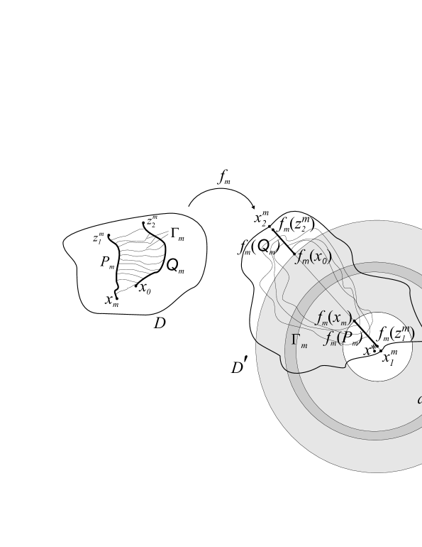
Figure 1: To the proof of Theorem 1

Since the domain $D^{\,\prime}$ is bounded, there are points $x_{1}^{m}$ and $x_{2}^{m}$ of intersection of the line $r_{m}$ with the boundary of the domain $D^{\,\prime},$ see, e.g., [Ku, Theorem 1.I.5.46]. Let $\gamma_{m}^{1}:[1,c_{m})\rightarrow D,$ $1<c_{m}\leqslant\infty,$ be a maximal $f_{m}$-lifting of $r=r(t),$ $t\geqslant 1,$ starting at $x_{m},$ existing by [MRV₂, Lemma 3.12]. By the same lemma

$$h(\gamma_{m}^{1}(t),\partial D)\rightarrow 0$$ (2.2)

as $t\rightarrow c_{m}-0.$ Similarly, let $\gamma_{m}^{2}:(d_{m},0]\rightarrow D,$ $-\infty\leqslant d_{m}<0$ be a maximal $f_{m}$-lifting of $r=r_{m}(t),$ $t\leqslant 0,$ ending at $x_{0},$ which exists by [MRV₂, Lemma 3.12]. As in (2.2), we have that

$$h(\gamma_{m}^{2}(t),\partial D)\rightarrow 0$$ (2.3)

as $t\rightarrow d_{m}+0.$ By (2.2) and (2.3), there exist $1\leqslant t_{m}^{1}<c_{m}$ i $d_{m}\leqslant t_{m}^{2}<0$ such that $h(z_{1}^{m},\partial D)<1/m$ and $h(z_{2}^{m},\partial D)<1/m,$ where $\gamma_{m}^{1}(t_{m}^{1})=z_{1}^{m}$ and $\gamma_{m}^{2}(t_{m}^{2})=z_{2}^{m}.$ Set $P_{m}=\gamma_{m}^{1}|_{[1,t_{m}^{1}]},$ $Q_{m}=\gamma_{m}^{2}|_{[t_{m}^{2},0]}$ and $\Gamma_{m}:=\Gamma(P_{m},Q_{m},D).$ Since the inner points of any domain are weakly flat (see, e.g., [SevSkv, Lemma 2.2]), we obtain that

$$M(\Gamma_{m})=M(\Gamma(P_{m},Q_{m},D))\rightarrow\infty\,,\quad m\rightarrow\infty\,.$$ (2.4)

We show that condition (2.4) leads to a contradiction with the definition of the class of mappings ${\mathfrak{R}}_{Q}(D,D^{\,\prime})$ in (1.3). We denote

$$a_{m}:=|f_{m}(z_{1}^{m})-f_{m}(x_{m})|,\,b_{m}=|f_{m}(z_{1}^{m})-f_{m}(x_{0})|\,.$$

Obviously, by construction

$$f_{m}(P_{m})\subset B(f_{m}(z_{1}^{m}),a_{m})\,,$$

$$f_{m}(Q_{m})\subset{\mathbb{R}}^{n}\setminus B(f_{m}(z_{1}^{m}),b_{m})\,.$$ (2.5)

Since the domain $D^{\,\prime}$ is bounded, we may assume that all three sequences $f_{m}(z_{1}^{m}),$ $f_{m}(x_{0})$ and $f_{m}(x_{m})$ converge to some elements $\widetilde{x},$ $\widetilde{x_{1}}$ and $\widetilde{x_{2}}$ at $m\rightarrow\infty,$ respectively. Now $a_{m}\rightarrow a_{0}$ and $b_{m}\rightarrow b_{0}$ as $m\rightarrow\infty,$ where $a_{0}=|\widetilde{x}-\widetilde{x_{2}}|$ and $b_{0}=|\widetilde{x}-\widetilde{x_{1}}|.$

Fix

$$0<\varepsilon<\varepsilon_{0}/2\,.$$ (2.6)

Let $x^{\,*}\in D$ be such that $|x^{\,*}-\widetilde{x}|<\varepsilon/3.$ Besides that, let $m_{0}\in{\mathbb{N}}$ be such that

$$|f_{m}(z_{1}^{m})-\widetilde{x}|<\varepsilon/3\,,\quad a_{0}-\varepsilon/3<a_{m}<a_{0}+\varepsilon/3\quad\forall\,\,m>m_{0}\,.$$ (2.7)

Let $x\in B(f_{m}(z_{1}^{m}),a_{m}).$ Now, by (2.7) and the triangle inequality we obtain that

$$|x-x^{\,*}|\leqslant|x-f_{m}(z_{1}^{m})|+|f_{m}(z_{1}^{m})-\widetilde{x}|+|\widetilde{x}-x^{\,*}|<$$

$$<a_{m}+\varepsilon/3+\varepsilon/3<a_{0}+\varepsilon\,,\quad m>m_{0}\,.$$ (2.8)

It follows from (2.8) that

$$B(f_{m}(z_{1}^{m}),a_{m})\subset B(x^{\,*},a_{0}+\varepsilon)\,,\quad m>m_{0}\,.$$ (2.9)

Let $R_{0}$ be such that

$$a_{0}+\varepsilon<R_{0}<a_{0}+\varepsilon_{0}-\varepsilon\,.$$ (2.10)

Note that the choice of the number $R_{0}$ in the formula (2.10) is possible by the definition of the number $\varepsilon$ in (2.6). Let $y\in B(x^{\,*},R_{0}).$ Again, by the triangle inequality, and by (2.7) and (2.10) we obtain that

$$|y-f_{m}(z_{1}^{m})|\leqslant|y-x^{\,*}|+|x^{\,*}-\widetilde{x}|+|\widetilde{x}-f_{m}(z_{1}^{m})|<$$

$$<R_{0}+2\varepsilon/3<a_{0}+\varepsilon_{0}-\varepsilon+2\varepsilon/3=a_{0}+\varepsilon_{0}-\varepsilon/3<a_{m}+\varepsilon_{0}\leqslant b_{m}\,.$$ (2.11)

It follows from (2.11) that

$$B(x^{\,*},R_{0})\subset B(f_{m}(z_{1}^{m}),b_{m})\,,\quad m>m_{0}\,.$$ (2.12)

Taking into account relations (2.5), (2.9) and (2.12), as well as [Ku, Theorem 1.I.5.46], we obtain that

$$\Gamma_{m}>\Gamma_{f_{m}}(x^{\,*},a_{0}+\varepsilon,R_{0})\,,\quad m>m_{0}\,.$$ (2.13)

In turn, from relation (2.13), as well as from the definition of the class $\mathfrak{R}_{Q}(D,D^{\,\prime}),$ it follows that

$$M(\Gamma_{m})\leqslant M(\Gamma_{f_{m}}(x^{\,*},a_{0}+\varepsilon,R_{0}))\leqslant\int\limits_{A}Q(y)\cdot\eta^{n}(|y-x^{\,*}|)\,dm(y)\,,\quad m>m_{0}\,,$$ (2.14)

where $A=A(x^{\,*},a_{0}+\varepsilon,R_{0}),$ and $\eta$ is an arbitrary non-negative Lebesgue measurable function satisfying condition (1.4) for $r_{1}=a_{0}+\varepsilon$ and $r_{2}=R_{0}.$ Below we use the standard conventions $a/\infty=0$ for $a\neq\infty$ and $a/0=\infty$ if $a>0$ and $0\cdot\infty=0$ (see e.g. [Sa, 3.I]). Put now

$$I=\int\limits_{a_{0}+\varepsilon}^{R_{0}}\frac{dt}{tq_{x^{\,*}}^{1/(n-1)}(t)}\,,$$ (2.15)

where

$$q_{y_{0}}(r)=\frac{1}{\omega_{n-1}r^{n-1}}\int\limits_{S(y_{0},r)}Q(y)\,d\mathcal{H}^{n-1}(y)\,,$$ (2.16)

$\omega_{n-1}$ is the area of the unit sphere ${\mathbb{S}}^{n-1}$ in ${\mathbb{R}}^{n},$ and $q_{x^{\,*}}(t)$ is defined in (2.16) for $y_{0}:=x^{\,*}.$ By the hypothesis of the theorem, there is a set $E\subset[a_{0}+\varepsilon,R_{0}]$ of positive linear measure such that the function $q_{x^{\,*}}(t)$ is finite for $t\in E.$ Thus, $I\neq 0$ in (2.15). In this case, the function $\eta_{0}(t)=\frac{1}{Itq_{x^{\,*}}^{1/(n-1)}(t)}$ satisfies (1.4) for $r_{1}=a_{0}+\varepsilon$ and $r_{2}=R_{0}.$ Substituting this function on the right side of the inequality (2.14) and applying Fubini’s theorem, we obtain

$$M(\Gamma_{m})\leqslant\frac{\omega_{n-1}}{I^{n-1}}<\infty\,,\quad m>m_{0}\,,$$ (2.17)

where $\omega_{n-1}$ is the area of the unit sphere ${\mathbb{S}}^{n-1}$ in ${\mathbb{R}}^{n}.$ However, relation (2.17) contradicts (2.4). The obtained contradiction refutes the assumption made in (2.1). $\Box$

To illustrate Theorem 1, we consider the following examples.

Example 1. This example is devoted to the study of the case when the result of Theorem 1 (Corollary 1) can be applied to some family of mappings, although the corresponding function $Q$ is not integrable in the domain under consideration. In this case, however, the so-called Lehto type integral diverges for the function $Q$ (see e.g. [MRSY₂, (7.50)]). We consider the following function $\varphi:(0,1]\rightarrow{\mathbb{R}},$ defined as follows:

$$\varphi(t)=\left\{\begin{array}[]{rr}1,&t\in\left(\frac{1}{2k+1},\frac{1}{2k}\right),\,k=1,2,\ldots\,,\\ \frac{1}{t^{n}},&t\in\left[\frac{1}{2k},\,\frac{1}{2k-1}\right],\,k=1,2,\ldots\,,\end{array}\right.$$

$$Q(x)=\varphi(|x|)\,,\quad Q:\overline{{\mathbb{B}}^{n}}\setminus\{0\}\rightarrow[0,\infty)\,.$$ (2.18)

As usual, put

$$q_{0}(t)=\frac{1}{\omega_{n-1}t^{n-1}}\int\limits_{S(0,t)}Q(x)\,d\mathcal{H}^{n-1}(x)\,.$$

Using the Fubini theorem, as well as the countable additivity of the Lebesgue integral, we will have:

$$\int\limits_{{\mathbb{B}}^{n}}Q(x)\,dm(x)=\int\limits_{0}^{1}\int\limits_{S(0,r)}Q(x)\,d\mathcal{H}^{n-1}dr=$$

$$=\omega_{n-1}\int\limits_{0}^{1}r^{n-1}\varphi(r)\,dr\geqslant\omega_{n-1}\sum\limits_{k=1}^{\infty}\int\limits_{1/(2k)}^{1/(2k-1)}\frac{dr}{r}=\omega_{n-1}\sum\limits_{k=1}^{\infty}\ln\left(\frac{2k}{2k-1}\right)\,.$$ (2.19)

Note that the series on the right-hand side of (2.19) diverges. Indeed, by virtue of the Lagrange’s mean value theorem $\ln\left(\frac{2k}{2k-1}\right)=\ln(2k)-\ln(2k-1)=\frac{1}{\theta(k)}\geqslant\frac{1}{2k},$ where $\theta(k)\in[2k-1,2k].$ Since $\sum\limits_{k=1}^{\infty}\frac{1}{2k}=\infty,$ we obtain that $\sum\limits_{k=1}^{\infty}\ln\left(\frac{2k}{2k-1}\right)=\infty$ and, consequently,

$$\int\limits_{{\mathbb{B}}^{n}}Q(x)\,dm(x)=\infty\,.$$

On the other hand,

$$\int\limits_{0}^{1}\frac{dt}{tq^{1/(n-1)}_{0}(t)}\geqslant\sum\limits_{k=1}^{\infty}\int\limits_{1/(2k+1)}^{1/(2k)}\frac{dr}{r}=\sum\limits_{k=1}^{\infty}\ln\frac{2k+1}{2k}=\infty\,.$$ (2.20)

Define a sequence of mappings $f_{m}:{\mathbb{B}}^{n}\rightarrow{\mathbb{R}}^{n}$ by

$$f_{m}(x)=\frac{x}{|x|}\,\rho_{m}(|x|)\,,\qquad f_{m}(0):=0\,,$$

where

$$\rho_{m}(r)=\exp\left\{-\int\limits_{r}^{1}\frac{dt}{tq_{0,m}^{1/(n-1)}(t)}\right\}\,,\qquad q_{0,m}(r):=\frac{1}{\omega_{n-1}r^{n-1}}\int\limits_{|x|=r}Q_{m}(x)\,dS\,,$$

$$Q_{m}(x)\quad=\quad\left\{\begin{array}[]{rr}Q(x),&\ |x|>1/m\ ,\\ 1\ ,&|x|\leq 1/m\,.\end{array}\right.$$

Note that each of the mappings $f_{m}$ is a homeomorphism of the unit ball ${\mathbb{B}}^{n}$ onto itself. Now we show that every $f_{m},$ $m=1,2,\ldots,$ satisfies the relation (1.9) where the function $Q$ defined by (2.18). First of all, we note that each mapping $f_{m}$ belongs to the class $ACL$; moreover, their norm and Jacobian are calculated by the relations

$$\|f_{m}^{\,\prime}(x)\|=\frac{\exp\left\{-\int\limits_{|x|}^{1}\frac{dt}{tq_{0,m}^{1/(n-1)}(t)}\right\}}{|x|},\quad|J(x,f_{m})|=\frac{\exp\left\{-n\int\limits_{|x|}^{1}\frac{dt}{tq_{0,m}^{1/(n-1)}(t)}\right\}}{|x|^{n}q_{0,m}^{1/(n-1)}(|x|)}\,,$$

see [IS, Proof of Theorem 5.2]. Thus, $f_{m}\in W_{\rm loc}^{1,n}({\mathbb{B}}^{n}\setminus 0).$ Moreover, the so-called inner dilatation $K_{I}(x,f_{m})$ of $f_{m}$ at the point $x$ is calculated as $K_{I}(x,f_{m})=q_{0,m}(|x|)\leqslant q_{0}(|x|),$ where $q_{0,m}(r)=\frac{1}{\omega_{n-1}r^{n-1}}\int\limits_{S(0,r)}Q_{m}(x)\,d\mathcal{H}^{n-1}(x)$ (see ibid.). In this case, $f_{m}$ satisfy relation (1.9) with $Q=K_{I}(x,f)=q_{0}(|x|)$ (see, for example, [MRSY₂, Corollary 8.5 and Theorem 8.6].

Note that the function $Q,$ extended by zero outside the unit ball, is integrable over almost all spheres centered at each point $x_{0}\in{\mathbb{B}}^{n},$ since this function is locally bounded in ${\mathbb{B}}^{n}\setminus\{0\}.$ Thus, the maps $g_{m}=f_{m}^{\,-1},$ $m=1,2,\ldots$ satisfy all the conditions of Corollary 1 (more generally, Theorem 1), and by this Corollary the family of mappings $\{g_{m}\}_{m=1}^{\infty}$ is equicontinuous in the unit ball. Moreover, the function $Q$ is not integrable in the unit ball due to relation (2.19), however, the family $\{f_{m}\}_{m=1}^{\infty}$ is equicontinuous in ${\mathbb{B}}^{n}$ due to condition (2.20) and [MRSY₂, Theorem 7.6]. However, the equicontinuity of the family $\{f_{m}\}_{m=1}^{\infty}$ can be verified directly; moreover, the equicontinuity of the inverse family $\{g_{m}\}_{m=1}^{\infty}$ may be obtained from the fact that $f_{m}$ converges to some homeomorphism $f$ as $m\rightarrow\infty$ locally uniformly. In this case, $g_{m}$ also converges locally uniformly to some homeomorphism $g=f^{\,-1}$ (see [RSS₁, Lemma 3.1]).

Example 2. Now consider the sequence of functions

$$Q_{m}(x)\quad=\quad\left\{\begin{array}[]{rr}\frac{1}{|x|^{n}},&\ |x|>1/m\ ,\\ 1\ ,&|x|\leqslant 1/m\,.\end{array}\right.$$

In the same way as above, we put

$$f_{m}(x)=\frac{x}{|x|}\,\rho_{m}(|x|)\,,\qquad f_{m}(0):=0\,,$$

where

$$\rho_{m}(r)=\exp\left\{-\int\limits_{r}^{1}\frac{dt}{tq_{0,m}^{1/(n-1)}(t)}\right\}\,,\qquad q_{0,m}(r):=\frac{1}{\omega_{n-1}r^{n-1}}\int\limits_{|x|=r}Q_{m}(x)\,dS\,,$$

Note that the mappings $f_{m},$ as well as inverse mappings $g_{m}:=f^{\,-1}_{m}$ can be written in explicit form, namely,

$$f_{m}(x)\quad=\quad\left\{\begin{array}[]{rr}mx\cdot\exp\{\frac{n-1}{n}\cdot((1/m)^{n/(n-1)}-1\},&\ |x|\leqslant 1/m\ ,\\ \frac{x}{|x|}\exp\{\frac{n-1}{n}\cdot(|x|^{n/(n-1)}-1)\}\ ,&|x|>1/m\,,\end{array}\right.$$

$$g_{m}(y)=\left\{\begin{array}[]{rr}\frac{y}{m}\cdot\exp\{\frac{1-n}{n}((1/m)^{n/(n-1)}-1\},&\ |y|\leqslant\exp\{\frac{n-1}{n}\cdot((1/m)^{n/(n-1)}-1)\}\ ,\\ \frac{y}{|y|}\cdot\frac{(n\ln|y|+(n-1))^{(n-1)/n}}{(n-1)^{(n-1)/n}}\ ,&|y|>\exp\{\frac{n-1}{n}\cdot((1/m)^{n/(n-1)}-1)\}\,.\end{array}\right.$$

Reasoning as in Example 2, it can be shown that the maps $f_{m}$ satisfy relation (1.9) for $D={\mathbb{B}}^{n}$ and $Q(x)=\frac{1}{|x|^{n}}.$ Note that $\int\limits_{{\mathbb{B}}^{n}}Q(x)\,dm(x)=\infty,$ although in this case we have $\int\limits_{0}^{1}\frac{dt}{tq_{0}^{1/(n-1)}(t)}<\infty.$ Note that, in contrast to the mappings from Example 2, we have a locally uniform convergence of $g_{m}$ to $g$ as $m\rightarrow\infty,$ where $g$ is some continuous mapping. Moreover, the ’’direct’’ sequence of mappings of $f_{m},$ $m=1,2,\ldots,$ is neither convergent, nor equicontinuous, in ${\mathbb{B}}^{n}.$ This fact about the equicontinuity of the maps $g_{m}$ is also the result of Corollary 1 (Theorem 1), since the function $Q$ has finite mean values over almost all spheres.

3 Logarithmic Hölder continuity of mappings of the unit ball

Proof of Theorem 1. We fix $x,y\in K\subset{\mathbb{B}}^{n}$ and $f\in\mathfrak{F}_{Q}({\mathbb{B}}^{n}).$ Put

$$|f(x)-f(y)|:=\varepsilon_{0}\,.$$ (3.1)

If $\varepsilon_{0}=0,$ there is nothing to prove. Let $\varepsilon_{0}>0.$ Draw through the points $f(x)$ and $f(y)$ a straight line $r=r(t)=f(x)+(f(x)-f(y))t,$ $-\infty<t<\infty$ (see Figure 2).

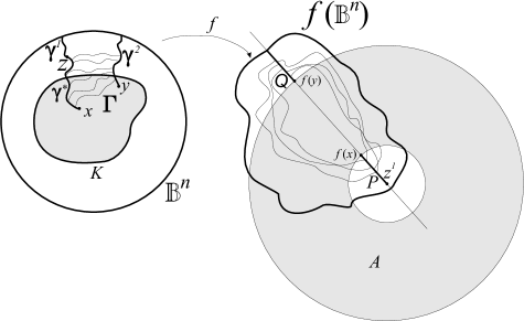
Figure 2: To proof of Theorem 1

Let $\gamma^{1}:[1,c)\rightarrow{\mathbb{B}}^{n},$ $1<c\leqslant\infty$ be a maximal $f$-lifting of the ray $r=r(t),$ $t\geqslant 1,$ starting at $x,$ which exists by [MRV₂, Lemma 3.12]. By the same lemma

$$h(\gamma^{1}(t),\partial{\mathbb{B}}^{n})\rightarrow 0$$ (3.2)

as $t\rightarrow c-0.$ Similarly, let $\gamma^{2}:(d,0]\rightarrow{\mathbb{B}}^{n},$ $-\infty\leqslant d<0$ be a maximal $f$-lifting of the ray $r=r(t),$ $t\leqslant 0,$ with end at a point $y,$ which exists by [MRV₂, Lemma 3.12]. Just like in (3.2) we have that

$$h(\gamma^{2}(t),\partial{\mathbb{B}}^{n})\rightarrow 0$$

as $t\rightarrow d+0.$ Let $z=\gamma_{1}(t_{1})$ be some point on the path $\gamma_{1}$ located at the distance $r_{0}/2$ from the boundary of the unit ball, where $r_{0}:=d(K,\partial{\mathbb{B}}^{n}).$ Put $\gamma^{*}(t):=\gamma_{1}|_{[1,t_{1}]}.$ Now, by the triangle inequality, ${\rm diam}\,(|\gamma^{*}(t)|)\geqslant r_{0}/2.$ By [Vu₂, Lemma 4.3]

$$M(\Gamma)\geqslant(1/2)\cdot M(\Gamma(|\gamma^{*}|,|\gamma^{2}|,{\mathbb{R}}^{n}))\,,$$ (3.3)

and on the other hand, by [Vu₁, Lemma 7.38]

$$M(\Gamma(|\gamma^{*}|,|\gamma^{2}|,{\mathbb{R}}^{n}))\geqslant c_{n}\cdot\log\left(1+\frac{1}{m}\right)\,,$$ (3.4)

where $c_{n}>0$ is some constant depending only on $n,$

$$m=\frac{{\rm dist}(|\gamma^{*}|,|\gamma^{2}|)}{\min\{{\rm diam\,}(|\gamma^{*}|),{\rm diam\,}(|\gamma^{2}|)\}}\,.$$

Note that ${\rm diam}\,(|\gamma^{i}|)=\sup\limits_{x,y\in|\gamma^{i}|}|x-y|\geqslant r_{0}/2,$ $i=1,2.$ Then combining (3.3) and (3.4), and taking into account that ${\rm dist}\,(|\gamma^{*}|,|\gamma^{2}|)\leqslant|x-x_{0}|,$ we obtain that

$$M(\Gamma)\geqslant\widetilde{c_{n}}\cdot\log\left(1+\frac{r_{0}}{2{\rm dist}(|\gamma^{*}|,|\gamma^{2}|)}\right)\geqslant\widetilde{c_{n}}\cdot\log\left(1+\frac{r_{0}}{2|x-x_{0}|}\right)\,,$$ (3.5)

where $\widetilde{c_{n}}>0$ is some constant depending only on $n.$

Now let us prove the upper bound for $M(\Gamma).$ Let $z_{1}:=f(z),$ $P=|f(\gamma^{*})|$ and $Q=|f(\gamma^{2})|.$ Put

$$A:=A(z^{1},\varepsilon^{1},\varepsilon^{2})=\{x\in{\mathbb{R}}^{n}:\varepsilon^{1}<|x-z^{1}|<\varepsilon^{2}\}\,,$$

where $\varepsilon^{1}:=|f(x)-z^{1}|,$ $\varepsilon^{2}:=|f(y)-z^{1}|.$ We show that

$$f(\Gamma)>\Gamma(S(z^{1},\varepsilon^{1}),S(z^{1},\varepsilon^{2}),A)\,.$$ (3.6)

Indeed, let $\gamma\in\Gamma.$ Then $f(\gamma)\in f(\Gamma),$ $f(\gamma)=f(\gamma(s)):[0,1]\rightarrow{\mathbb{R}}^{n},$ $f(\gamma(0))\in P,$ $f(\gamma(1))\in Q$ and $f(\gamma(s))\in f({\mathbb{B}}^{n})$ for $0<s<1.$ Let $q>1$ be a number such that

$$z^{1}=f(y)+(f(x)-f(y))\,q.$$

Since $f(\gamma(0))\in P,$ there is $1\leqslant t\leqslant q$ such that $f(\gamma(0))=f(y)+(f(x)-f(y))t.$ So,

$$|f(\gamma(0))-z^{1}|=|(f(x)-f(y))(q-t)|\leqslant$$

$$\leqslant|(f(x)-f(y))(q-1)|=|(f(x)-f(y))q+f(y)-f(x))|=$$ (3.7)

$$=|f(x)-z^{1}|=\varepsilon^{1}\,.$$

On the other hand, since $f(\gamma(1))\in Q,$ there is $p\leqslant 0$ such that

$$f(\gamma(1))=f(y)+(f(x)-f(y))p\,.$$

In this case, we obtain that

$$|f(\gamma(1))-z^{1}|=|(f(x)-f(y))(q-p)|\geqslant$$

$$\geqslant|(f(x)-f(y))q|=|(f(x)-f(y))q+f(y)-f(y)|=$$ (3.8)

$$=|f(y)-z^{1}|=\varepsilon^{2}\,.$$

Observe that

$$|f(y)-f(x)|+\varepsilon^{1}=$$

$$=|f(y)-f(x)|+|f(x)-z^{1}|=|z^{1}-f(y)|=\varepsilon^{2}\,,$$ (3.9)

and, thus, $\varepsilon^{1}<\varepsilon^{2}.$ Now, by (3.8) we obtain that

$$|f(\gamma(1))-z^{1}|>\varepsilon^{1}\,.$$ (3.10)

It follows from (3.7) and (3.10) that $|f(\gamma)|\cap\overline{B(z^{1},\varepsilon^{1})}\neq\varnothing\neq(f({\mathbb{B}}^{n})\setminus\overline{B(z^{1},\varepsilon^{1})})\cap|f(\gamma)|.$ In this case, by [Ku, Theorem 1.I.5.46] there is $t_{1}\in(0,1)$ such that $f(\gamma(t_{1}))\in S(z^{1},\varepsilon^{1}).$ We may assume that $f(\gamma(t))\not\in B(z^{1},\varepsilon^{1})$ for $t\in(t_{1},1).$ Put $\alpha^{1}:=f(\gamma)|_{[t_{1},1]}.$

On the other hand, since $\varepsilon^{1}<\varepsilon^{2}$ and $f(\gamma(t_{1}))\in S(z^{1},\varepsilon^{1}),$ we obtain that $|\alpha^{1}|\cap B(z^{1},\varepsilon^{2})\neq\varnothing.$ By (3.8) we obtain that $(f({\mathbb{B}}^{n})\setminus B(z^{1},\varepsilon^{2}))\cap|\alpha^{1}|\neq\varnothing.$ Thus, by [Ku, Theorem 1.I.5.46] there is $t_{2}\in(t_{1},1)$ such that $\alpha^{1}(t_{2})\in S(z^{1},\varepsilon^{2}).$ We may assume that $f(\gamma(t))\in B(z^{1},\varepsilon^{2})$ for $t\in(t_{1},t_{2}).$ Set $\alpha^{2}:=\alpha^{1}|_{[t_{1},t_{2}]}.$ Now, $f(\gamma)>\alpha^{2}$ and $\alpha^{2}\in\Gamma(S(z^{1},\varepsilon^{1}),S(z^{1},\varepsilon^{2}),A).$ Thus, (3.6) is proved.

It follows from (3.6) that $\Gamma>\Gamma_{f}(z^{1},\varepsilon^{1},\varepsilon^{2}).$ Now, we set

$$\eta(t)=\left\{\begin{array}[]{rr}\frac{1}{\varepsilon_{0}},&t\in[\varepsilon^{1},\varepsilon^{2}],\\ 0,&t\not\in[\varepsilon^{1},\varepsilon^{2}]\,.\end{array}\right.$$

Note that $\eta$ satisfies the relation (1.4) for $r_{1}=\varepsilon^{1}$ and $r_{2}=\varepsilon^{2}.$ Indeed, it follows from (3.1) and (3.9) that

$$r_{1}-r_{2}=\varepsilon^{2}-\varepsilon^{1}=|f(y)-z^{1}|-|f(x)-z^{1}|=$$

$$=|f(x)-f(y)|=\varepsilon_{0}\,.$$

Then $\int\limits_{\varepsilon^{1}}^{\varepsilon^{2}}\eta(t)\,dt=(1/\varepsilon_{0})\cdot(\varepsilon^{2}-\varepsilon^{1})\geqslant 1.$ By the inequality (3.6), and the relation (1.3), applied at the point $z^{1},$ we obtain that

$$M(\Gamma)\leqslant M(\Gamma_{f}(z^{1},\varepsilon^{1},\varepsilon^{2}))\leqslant$$

$$\leqslant\frac{1}{\varepsilon_{0}^{n}}\int\limits_{{\mathbb{R}}^{n}}Q(z)\,dm(z)=\frac{\|Q\|_{1}}{{|f(x)-f(y)|}^{n}}\,.$$ (3.11)

By (3.5) and (3.11), we obtain that

$$\widetilde{c_{n}}\cdot\log\left(1+\frac{r_{0}}{2|x-y|}\right)\leqslant\frac{\|Q\|_{1}}{{|f(x)-f(y)|}^{n}}\,.$$

From the latter ratio, the desired inequality (1.7) follows, while $C_{n}:={\widetilde{c_{n}}}^{-1/n}.$ $\Box$

4 On logarithmic Hölder type maps in arbitrary domains

As we indicated above, the problem of Hölder continuity for mappings of arbitrary domains has not yet been resolved. Nevertheless, under certain not too rough conditions, a result of this kind can be obtained from the main theorem of the previous section. In order to formulate and prove it, we carry out the following notation.

For domains $D,D^{\,\prime}\subset{\mathbb{R}}^{n},$ $n\geqslant 2,$ and a Lebesgue measurable function $Q:{\mathbb{R}}^{n}\rightarrow[0,\infty],$ $Q(x)\equiv 0$ for $x\not\in D,$ we define by $\mathfrak{A}_{Q}(D,D^{\,\prime})$ the family of all open discrete mappings $f:D\rightarrow D^{\,\prime}$ such that relation (1.3) holds at each point $y_{0}\in D^{\,\prime}.$ The following result holds.

Theorem 4.1. Let $n\geqslant 2,$ and let $Q\in L^{1}({\mathbb{R}}^{n}).$ Suppose that $K$ is a compact set in $D,$ and beside that, $D^{\,\prime}$ is bounded. Now, the inequality

$$|f(x)-f(y)|\leqslant\frac{C\cdot(\|Q\|_{1})^{1/n}}{\log^{1/n}\left(1+\frac{r_{0}}{2|x-y|}\right)}$$

holds for any $x,y\in K$ and any $f\in\mathfrak{A}_{Q}(D,D^{\,\prime}),$ where $\|Q\|_{1}$ denotes $L^{1}$-norm of $Q$ in ${\mathbb{R}}^{n},$ $C=C(n,K)>0$ is some constant depending only on $n$ and $K,$ and $r_{0}=d(K,\partial D).$

Proof.   First of all, we observe that the equality $\|Q\|_{1}=0$ cannot hold under the conditions of Theorem 4. Indeed, let $B(x_{0},r),$ $r>0,$ be an arbitrary ball lying strictly inside the domain $D.$ Let also $\varphi$ be the conformal mapping of the unit ball ${\mathbb{B}}^{n}$ onto the ball $B(x_{0},r).$ Applying the restriction of the mapping $\widetilde{f}:=f|_{B(x_{0},r)}$ and considering the auxiliary map $F:=\widetilde{f}\circ\varphi$, $F:{\mathbb{B}}^{n}\rightarrow D^{\,\prime},$ we conclude that it also satisfies condition (1.3) with the same $Q.$ Thus, by Theorem 1, $F$ satisfies estimate (1.7) for any compact set $K^{\,\prime}\subset{\mathbb{B}}^{n}.$ Now, since $F$ is open and discrete, $\|Q\|_{1}\neq 0,$ as required.

In view of what has been said, it suffices to establish that the expression

$$|f(x)-f(y)|\cdot\log^{1/n}\left(1+\frac{r_{0}}{2|x-y|}\right)$$

is upper bounded for all $x,y\in K.$

Suppose the contrary. Then there are $x_{m},y_{m}\in K$ and $f_{m}\in\mathfrak{A}_{Q}(D,D^{\,\prime})$ such that

$$|f_{m}(x_{m})-f_{m}(y_{m})|\cdot\log^{1/n}\left(1+\frac{r_{0}}{2|x_{m}-y_{m}|}\right)\geqslant m\,,\quad m=1,2,\ldots.$$ (4.1)

Since $K$ is compact set, we may assume that both sequences $x_{m},y_{m}$ are convergent to some points $x_{0},y_{0}\in K$ as $m\rightarrow\infty.$

Further, two cases are possible: $x_{0}=y_{0}$ and $x_{0}\neq y_{0}.$ First let $x_{0}\neq y_{0}.$ Then by the triangle inequality

$$|f_{m}(x_{m})-f_{m}(y_{m})|\leqslant|f_{m}(x_{m})|+|f_{m}(y_{m})|\leqslant C$$ (4.2)

for some $C>0$ and any $m\in{\mathbb{N}},$ because $D^{\,\prime}$ is bounded by the assumption. It follows from (4.2) that

$$|f_{m}(x_{m})-f_{m}(y_{m})|\cdot\log^{1/n}\left(1+\frac{r_{0}}{2|x_{m}-y_{m}|}\right)\leqslant$$

$$\leqslant C\cdot\log^{1/n}\left(1+\frac{r_{0}}{2|x_{m}-y_{m}|}\right)\rightarrow C\cdot\log^{1/n}\left(1+\frac{r_{0}}{2|x_{0}-y_{0}|}\right)<\infty\,,\quad m\rightarrow\infty\,.$$ (4.3)

Relation (4.3) contradicts assumption (4.1), so the case $x_{0}\neq y_{0}$ is impossible.

We now consider another case, namely, when $x_{0}=y_{0}.$ Note that in this case both sequences $x_{m}$ and $y_{m}$ belong to $B(x_{0},r_{0})$ for any $m>m_{0}$ and some $m_{0}\in{\mathbb{N}},$ while $\overline{B(x_{0},r_{0}/2)}\subset B(x_{0},r_{0})\subset D.$ Let $\psi$ be the conformal mapping of the unit ball ${\mathbb{B}}^{n}$ onto the ball $B(x_{0},r_{0}),$ namely, $\psi(x)=xr_{0}+x_{0},$ $x\in{\mathbb{B}}^{n}.$ In particular, $\psi^{\,-1}(B(x_{0},r_{0}/2))=B(0,1/2).$ Applying the restriction of the mapping $\widetilde{f}_{m}:=(f_{m})|_{B(x_{0},r_{0})}$ and considering the auxiliary maps $F_{m}:=\widetilde{f}_{m}\circ\psi,$ $F_{m}:{\mathbb{B}}^{n}\rightarrow D^{\,\prime},$ we conclude that it also satisfies condition (1.3) with the same $Q.$ Now, by Theorem 1

$$|F_{m}(\psi^{\,-1}(x_{m}))-F_{m}(\psi^{\,-1}(y_{m}))|\leqslant\frac{C\cdot(\|Q\|_{1})^{1/n}}{\log^{1/n}\left(1+\frac{1}{4|\psi^{\,-1}(x_{m})-\psi^{\,-1}(y_{m})|}\right)}\,,\quad m>m_{0}\,.$$ (4.4)

Since $F_{m}(\psi^{\,-1}(x_{m}))=f_{m}(x_{m})$ and $F_{m}(\psi^{\,-1}(y_{m}))=f_{m}(y_{m}),$ we may rewrite (4.4) as

$$|f_{m}(x_{m})-f_{m}(y_{m})|\leqslant\frac{C\cdot(\|Q\|_{1})^{1/n}}{\log^{1/n}\left(1+\frac{1}{4|\psi^{\,-1}(x_{m})-\psi^{\,-1}(y_{m})|}\right)}\,,\quad m>m_{0}\,.$$ (4.5)

Note that the maps $\psi^{\,-1}(y)$ are Lipschitz with the Lipschitz constant $\frac{1}{r_{0}}.$ In this case, we obtain from relation (4.5) that

$$|f_{m}(x_{m})-f_{m}(y_{m})|\leqslant\frac{C\cdot(\|Q\|_{1})^{1/n}}{\log^{1/n}\left(1+\frac{r_{0}}{4|x_{m}-y_{m}|}\right)}\,,\quad m>m_{0}\,.$$ (4.6)

Finally, we note that $\log^{1/n}\left(1+\frac{1}{nt}\right)\sim\log^{1/n}\left(1+\frac{1}{kt}\right)$ as $t\rightarrow+0$ for various fixed $k,n>0,$ which may be verified using the L’Hôpital rule. It follows that

$$\frac{C\cdot(\|Q\|_{1})^{1/n}}{\log^{1/n}\left(1+\frac{r_{0}}{4|x_{m}-y_{m}|}\right)}\leqslant\frac{C_{1}\cdot(\|Q\|_{1})^{1/n}}{\log^{1/n}\left(1+\frac{r_{0}}{2|x_{m}-y_{m}|}\right)}$$

for some constant $C_{1}>0,$ some $m_{1}\in{\mathbb{N}}$ and any $m>m_{1}>m_{0}.$ In this case, it follows from (4.6) that

$$|f_{m}(x_{m})-f_{m}(y_{m})|\leqslant\frac{C_{1}\cdot(\|Q\|_{1})^{1/n}}{\log^{1/n}\left(1+\frac{r_{0}}{2|x_{m}-y_{m}|}\right)}\,,\quad m>m_{1}\,.$$ (4.7)

However, relation (4.7) contradicts (4.1). The obtained contradiction proves the theorem. $\Box$

5 Applications to the Beltrami equation

Recently, the topic related to the existence of solutions of degenerate Beltrami differential equations has been actively developed (see, e.g., [RSY₁], [RSY₂], [GRY], and [GRSY]). The main results on this topic are compiled in a relatively recent monograph [GRSY], with links to publications by these and other authors. One of the problems posed in the study of Beltrami equations is to find the conditions for a complex coefficient that ensure that their solutions exist. Finding solutions is usually is carried out in the class of $ACL$-homeomorphisms, although it is quite correct to consider just continuous $ACL$-solutions. In this section, we obtain another result on the existence of solutions of degenerate Beltrami equation, which is based on the transition to inverse mappings. Compared to [RSY₁], [RSY₂] and [GRY] , we are somewhat weakening the conditions on a complex coefficient. The obtained solution of the equation may not be homeomorphic, but relative to the previous results, the degree of its smoothness is $W_{\rm loc}^{1,p},$ $p>1,$ and therefore somewhat higher.

We turn now to the definitions. Let $D$ be a domain in ${\mathbb{C}}.$ In what follows, a mapping $f:D\rightarrow{\mathbb{C}}$ is assumed to be sense-preserving, moreover, we assume that $f$ has partial derivatives almost everywhere. Put $f_{\overline{z}}=\left(f_{x}+if_{y}\right)/2$ and $f_{z}=\left(f_{x}-if_{y}\right)/2.$ The complex dilatation of $f$ at $z\in D$ is defined as follows: $\mu(z)=\mu_{f}(z)=f_{\overline{z}}/f_{z}$ for $f_{z}\neq 0$ and $\mu(z)=0$ otherwise. The maximal dilatation of $f$ at $z$ is the following function:

$$K_{\mu}(z)=K_{\mu_{f}}(z)=\quad\frac{1+|\mu(z)|}{1-|\mu\,(z)|}\,.$$ (5.1)

Note that the Jacobian of $f$ at $z\in D$ may be calculated according to the relation

$$J(z,f)=|f_{z}|^{2}-|f_{\overline{z}}|^{2}\,.$$

Since we assume that the map $f$ is sense preserving, the Jacobian of this map is positive at all points of its differentiability. Let ${\mathbb{D}}=\{z\in{\mathbb{C}}:|z|<1\},$ and let $\mu:D\rightarrow{\mathbb{D}}$ be a Lebesgue measurable function. Without reference to some mapping $f,$ we define the maximal dilatation corresponding to its complex dilatation $\mu$ by (5.1). It is easy to see that

$$K_{\mu_{f}}(z)=\frac{|f_{z}|+|f_{\overline{z}}|}{|f_{z}|-|f_{\overline{z}}|}$$

whenever partial derivatives of $f$ exist at $z\in D$ and, in addition, $J(z,f)\neq 0.$ We also define the inner dilatation of the order $p\geqslant 1$ of the map $f$ by the relation

$$K_{I,p}(z,f)=\frac{{|f_{z}|}^{2}-{|f_{\overline{z}}|}^{2}}{{(|f_{z}|-|f_{\overline{z}}|)}^{p}}$$ (5.2)

whenever $J(z,f)\neq 0,$ in addition, we set $K_{I,p}(z)=1$ provided that $|f_{z}|+|f_{\overline{z}}|=0,$ and $K_{I,p}(z)=\infty$ when $J(z,f)=0,$ but $|f_{z}|+|f_{\overline{z}}|\neq 0.$ Observe that $K_{I,2}(z)=K_{\mu}(z).$ Set $\|f^{\,\prime}(z)\|=|f_{z}|+|f_{\overline{z}}|.$ Recall that a homeomorphism $f:D\rightarrow{\mathbb{C}}$ is said to be quasiconformal if $f\in W_{\rm loc}^{1,2}(D)$ and, in addition, $\|f^{\,\prime}(z)\|^{2}\leqslant K\cdot|J(z,f)|$ for some constant $K\geqslant 1.$

We will call the Beltrami equation the differential equation of the form

$$f_{\overline{z}}=\mu(z)\cdot f_{z}\,,$$ (5.3)

where $\mu=\mu(z)$ is a given function with $|\mu(z)|<1$ a.a. Given $k\geqslant 1$ we set

$$\mu_{k}(z)=\left\{\begin{array}[]{rr}\mu(z),&K_{\mu}(z)\leqslant k,\\ 0\ ,&K_{\mu}(z)>k\,.\end{array}\right.$$ (5.4)

Let $f_{k}$ be a homeomorphic $ACL$-solution of the equation $f_{\overline{z}}=\mu_{k}(z)\cdot f_{z},$ which maps the unit disk onto itself and satisfies the normalization conditions $f_{k}(0)=0,$ $f_{k}(1)=1.$ This a solution exists by [A, Theorem 3.B.V] or [Bo, Theorem 8.2]. Note that the inverse mapping $g_{k}=f^{\,-1}_{k}$ is quasiconformal; in particular, it is differentiable almost everywhere (see, for example, [BI, Theorems 5.3 and 9.1]). Let $g_{k}$ be a inverse mapping to $f_{k},$ then its complex dilation $\mu_{g_{k}}$ is calculated according to the relation $\mu_{g_{k}}(w)=-\mu_{k}(g_{k}(w))=-\mu_{k}(f^{\,-1}_{k}(w)),$ see e.g., [A, (4).C.I]. In this case, the maximal dilation of $g_{k}$ is calculated by the relation

$$K_{\mu_{g_{k}}}(w)=\quad\frac{1+|\mu_{k}(f^{\,-1}_{k}(w))|}{1-|\mu_{k}(f^{\,-1}_{k}(w))|}\,.$$ (5.5)

Accordingly, the inner dilatation of the order $p$ of the map $g_{k}$ can be calculated according to relation (5.2), namely,

$$K_{I,p}(w,g_{k})=\frac{{|(g_{k})_{w}|}^{2}-{|(g_{k})_{\overline{w}}|}^{2}}{{(|(g_{k})_{w}|-|(g_{k})_{\overline{w}}|)}^{p}}\,.$$ (5.6)

Let $\Omega_{n}$ be a volume of the unit ball ${\mathbb{B}}^{n}$ in ${\mathbb{R}}^{n}.$ Suppose that a function ${\varphi}:D\rightarrow{\mathbb{R}}$ is locally integrable in some neighborhood of a point $x_{0}\in D.$ We say that ${\varphi}$ has a finite mean oscillation at $x_{0}\in D,$ write $\varphi\in FMO(x_{0}),$ if the relation

$${\limsup\limits_{\varepsilon\rightarrow 0}}\,\frac{1}{\Omega_{n}\varepsilon^{n}}\int\limits_{B(x_{0},\,\varepsilon)}|{\varphi}(x)-\overline{{\varphi}}_{\varepsilon}|\ dm(x)\,<\,\infty$$

holds, where $\overline{{\varphi}}_{\varepsilon}=\frac{1}{\Omega_{n}\varepsilon^{n}}\int\limits_{B(x_{0},\,\varepsilon)}{\varphi}(x)\ dm(x)$ (see, e.g., [RSY₂, section 2]). We say that a function $\varphi$ has a finite mean oscillation in $D,$ write $\varphi\in FMO(D),$ if $\varphi\in FMO(x_{0})$ for any $x_{0}\in D.$ The following statement holds.

Theorem 5.1.  Let $g_{k}=f_{k}^{\,-1}$ and $f_{k}$ be a homeomorphic $ACL$-solution of the equation $f_{\overline{z}}=\mu_{k}(z)\cdot f_{z},$ that maps the unit disk onto itself and satisfies the normalization conditions $f_{k}(0)=0,$ $f_{k}(1)=1$; moreover, let $\mu_{k}(z)$ be given by the relation (5.4). Suppose that the functions $Q:{\mathbb{D}}\rightarrow[1,\infty]$ and $\mu:{\mathbb{D}}\rightarrow{\mathbb{D}}$ are Lebesgue measurable, in addition, assume that the following conditions hold:

1) for each $0<r_{1}<r_{2}<1$ and $y_{0}\in{\mathbb{D}}$ there is a set $E\subset[r_{1},r_{2}]$ of positive linear Lebesgue measure such that the function $Q$ is integrable over the circles $S(y_{0},r)$ for any $r\in E;$

2) there exist a number $1<p\leqslant 2$ and a constant $M>0$ such that

$$\int\limits_{{\mathbb{D}}}K_{I,p}(w,g_{k})\,dm(w)\leqslant M$$ (5.7)

for almost all $w\in{\mathbb{D}}$ and all $k=1,2,\ldots.$ where $K_{I,p}(z,g_{k})$ is defined in (5.6);

3) the inequality

$$K_{\mu_{g_{k}}}(w)\leqslant Q(w)$$ (5.8)

holds for a.e. $w\in{\mathbb{D}},$ where $K_{\mu_{g_{k}}}$ is defined in (5.5).

Then the equation (5.3) has a continuous $W_{\rm loc}^{1,p}({\mathbb{D}})$-solution $f$ in ${\mathbb{D}}.$

Corollary 5.1.   In particular, the conclusion of Theorem 5 holds if, in this theorem, the conditions on the function $Q$ are replaced by the condition $Q\in L^{1}({\mathbb{D}}).$ In this case, the solution $f$ of equation (5.3) can be chosen such that

$$|f(x)-f(y)|\leqslant\frac{C\cdot(\|Q\|_{1})^{1/n}}{\log^{1/n}\left(1+\frac{r_{0}}{2|x-y|}\right)}$$ (5.9)

for any compact set $K\subset{\mathbb{D}}$ and $x\in x,y\in K,$ where $\|Q\|_{1}$ denotes $L^{1}$-norm of $Q$ in ${\mathbb{D}},$ $C>0$ is some constant, and $r_{0}=d(K,\partial{\mathbb{D}}).$

Corollary 5.2. If, under the conditions of Corollary 5, we require in addition that either $Q(z)\in FMO({\mathbb{D}}),$ or

$$\int\limits_{0}^{\delta(w_{0})}\frac{dt}{tq_{w_{0}}(t)}=\infty$$ (5.10)

for any $w_{0}\in{\mathbb{D}}$ and some $\delta(w_{0})>0,$ $q_{w_{0}}(r)=\frac{1}{2\pi}\int\limits_{0}^{2\pi}Q(w_{0}+re^{\,i\theta})\,d\theta,$ then $f$ can be chosen as a homeomorphism in ${\mathbb{D}}.$

The proof of Theorem 5, as well as Corollaries 5 and 5, will be given later in the text. Before this, we formulate and prove the following most important convergence lemma. On this occasion, see also similar statements related to the study of equations and mappings with some another conditions, see, for example, [GRSY, Ch. 2] and [RSY₃].

Lemma 5.1.   Let $\mu:D\rightarrow{\mathbb{D}}$ be a Lebesgue measurable function. Suppose that $f_{k},$ $k=1,2,\ldots$ is a sequence of sense-preserving $W_{\rm loc}^{1,2}(D)$-homeomorphisms of $D$ onto itself with complex coefficients $\mu_{k}(z).$ Suppose that $f_{k}$ converges locally uniformly in $D$ to some mapping $f:D\rightarrow{\mathbb{C}}$ as $k\rightarrow\infty,$ and the sequence $\mu_{k}(z)$ converges to $\mu$ as $k\rightarrow\infty$ for almost all $z\in{\mathbb{D}}.$ Suppose also that the inverse mappings $g_{k}:=f_{k}^{\,-1}$ belong to the class $W_{\rm loc}^{1,2}(D)$ and, in addition,

$$\int\limits_{D}K_{I,p}(w,g_{k})\,dm(w)\leqslant M$$

for some $M>0,$ each $k=1,2,\ldots,$ and almost all $w\in D.$ Now $f\in W_{\rm loc}^{1,p}(D)$ and, in addition, $\mu$ is a complex characteristic of the map $f,$ in other words, $f_{\overline{z}}=\mu(z)\cdot f_{z}$ for almost all $z\in D.$

Proof.   In general, we will follow the scheme described in the proof of [RSY₃, Theorem 3.1], cf. [GRSY, Theorem 2.1] and [Re, Lemma III.3.5]. We denote $\partial f=f_{z}$ and $\overline{\partial}f=f_{\overline{z}}.$ Let $C$ be an arbitrary compact set in $D.$ Since, by assumption, the maps $g_{k}=f_{k}^{\,-1}$ belong to $W_{\rm loc}^{1,2},$ then $g_{k}$ possess the Luzin $N$-property (see, for example, [MM, Corollary B]). Now, the Jacobian $J(z,f)$ is almost everywhere nonzero, see, for example, [Pon, Theorem 1]. Since $f_{k}\in W_{\rm loc}^{1,2},$ a change of variables in the integral is true (see e.g. [Fe, Theorem 3.2.5]). In this case, we have that

$$\int\limits_{C}{\|f^{\,\prime}_{k}(z)\|}^{p}\,dm(z)=\int\limits_{C}\frac{{\|f^{\,\prime}_{k}(z)\|}^{p}}{J(z,f_{k})}\cdot J(z,f_{k})=$$

$$=\int\limits_{f_{k}(C)}K_{I,p}(w,g_{k})\,dm(w)\leqslant M<\infty\,.$$ (5.11)

It follows from (5.11) that $f\in W_{\rm loc}^{1,p},$ $\partial f_{k}$ and $\overline{\partial}f_{k}$ weakly converge in $L_{\rm loc}^{1}(D)$ to $\partial f$ and $\overline{\partial}f,$ respectively (see [RSY₃, Lemma 2.1] and [Re, Lemma III.3.5]).

It remains to show that the map $f$ is a solution of the Beltrami equation $f_{\overline{z}}=\mu(z)\cdot f_{z}.$ Put $\zeta(z)=\overline{\partial}f(z)-\mu(z)\partial f(z)$ and show that $\zeta(z)=0$ almost everywhere. Let $B$ be an arbitrary disk lying with its closure in $D.$ By the triangle inequality

$$\left|\int\limits_{B}\zeta(z)\,dm(z)\right|\leqslant I_{1}(k)+I_{2}(k)\,,$$ (5.12)

where

$$I_{1}(k)=\left|\int\limits_{B}(\overline{\partial}f(z)-\overline{\partial}f_{k}(z))\,dm(z)\right|$$ (5.13)

and

$$I_{2}(k)=\left|\int\limits_{B}(\mu(z)\partial f(z)-\mu_{k}(z)\partial f_{k}(z))\,dm(z)\right|\,.$$ (5.14)

By proved above, $I_{1}(k)\rightarrow 0$ as $k\rightarrow\infty.$ It remains to deal with the expression $I_{2}(k).$ To do this, note that $I_{2}(k)\leqslant I^{\,\prime}_{2}(k)+I^{\,\prime\prime}_{2}(k),$ where

$$I^{\,\prime}_{2}(k)=\left|\int\limits_{B}\mu(z)(\partial f(z)-\partial f_{k}(z))\,dm(z)\right|$$

and

$$I^{\,\prime\prime}_{2}(k)=\left|\int\limits_{B}(\mu(z)-\mu_{k}(z))\partial f_{k}(z)\,dm(z)\right|\,.$$

Due to the weak convergence of $\partial f_{k}\rightarrow\partial f$ in $L^{1}_{\rm loc}(D)$ as $k\rightarrow\infty,$ we obtain that $I^{\,\prime}_{2}(k)\rightarrow 0$ for $k\rightarrow\infty,$ since $\mu\in L^{\infty}(D).$ Moreover, for a given $\varepsilon>0$ there is $\delta=\delta(\varepsilon)>0$ such that

$$\int\limits_{E}|\partial f_{k}(z)|\,dm(z)\leqslant\int\limits_{E}|\partial f_{k}(z)-\partial f(z)|\,dm(z)+\int\limits_{E}|\partial f(z)|\,dm(z)<\varepsilon\,,$$ (5.15)

whenever $m(E)<\delta,$ $E\subset B,$ and $k$ is sufficiently large.

Finally, by Egorov’s theorem (see [Sa, Theorem III.6.12]) for each $\delta>0$ there exists a set $S\subset B$ such that $m(B\setminus S)<\delta$ and $\mu_{k}(z)\rightarrow\mu(z)$ uniformly on $S.$ Then $|\mu_{k}(z)-\mu(z)|<\varepsilon$ for all $k\geqslant k_{0},$ some $k_{0}=k_{0}(\varepsilon)\in{\mathbb{N}}$ and all $z\in S.$ Now, by (5.15) and (5.11), as well as Hölder’s inequality,

$$I^{\,\prime\prime}_{2}(k)\leqslant\varepsilon\int\limits_{S}|\partial f_{k}(z)|\,dm(z)+2\int\limits_{B\setminus S}|\partial f_{k}(z)|\,dm(z)<$$

$$<\varepsilon\cdot\left\{\left(\int\limits_{D}K_{I,p}(w,g_{k})\,dm(w)\right)^{1/p}\cdot(m(B))^{(p-1)/p}+2\right\}\leqslant$$ (5.16)

$$\leqslant\varepsilon\cdot\left(M^{1/p}\cdot(m(B))^{(p-1)/p}+2\right)\,.$$

for $k\geqslant k_{0}.$ From (5.12), (5.13), (5.14) and (5.16) it follows that $\int\limits_{B}\zeta(z)\,dm(z)=0$ for all disks $B,$ compactly embedded in $D.$ Based on the Lebesgue theorem on differentiation of an indefinite integral (see [Sa, IV(6.3)]), it follows that $\zeta(z)=0$ almost everywhere in $D.$ The lemma is proved. $\Box$

Proof of Theorem 5. Consider a sequence of complex-valued functions

$$\mu_{k}(z)=\left\{\begin{array}[]{rr}\mu(z),&K_{\mu}(z)\leqslant k,\\ 0\ ,&K_{\mu}(z)>k,\end{array}\right.$$ (5.17)

where $K_{\mu}(z)$ is defined by (5.1). Note that $\mu_{k}(z)\leqslant\frac{k-1}{k+1}<1,$ therefore, the equation (5.3), in which instead of $\mu$ on the right side we take $\mu:=\mu_{k},$ and $\mu_{k}$ is defined by the relation (5.17), has a homeomorphic $W_{\rm loc}^{1,2}({\mathbb{D}})$-solution $f_{k}:{\mathbb{D}}\rightarrow{\mathbb{D}}$ with normalizations $f_{k}(0)=0,$ $f_{k}(1)=1,$ which is $k$-quasiconformal in ${\mathbb{D}}$ (see [A, Theorem 3.B.V] or [Bo, Theorem 8.2]). By the same theorem, $f_{k}$ maps the unit disk onto itself; moreover, $g_{k}=f^{\,-1}_{k}$ are also quasiconformal, in particular, they belong to the class $W_{\rm loc}^{1,2}({\mathbb{D}}).$ By [MRSY₁, Theorem 6.10] and by (5.8)

$$M(g_{k}(\Gamma))\leqslant\int\limits_{\mathbb{D}}K_{\mu_{g_{k}}}(w)\cdot\rho_{*}^{2}(w)\,dm(w)\leqslant\int\limits_{\mathbb{D}}Q(w)\cdot\rho_{*}^{2}(w)\,dm(w)$$

for any $k\in{\mathbb{N}}$ and any path family $\Gamma$ in ${\mathbb{D}},$ and each function $\rho_{*}\in{\rm adm}\,\Gamma.$ By Theorem 1 the family $\{f_{k}\}_{k=1}^{\infty}$ is equicontinuous in ${\mathbb{D}}.$ Thus, by the Arzela-Ascoli theorem $f_{k}$ is a normal family of mappings (see e.g. [Va, Theorem 20.4]), in other words, there is a subsequence $f_{k_{l}}$ of $f_{k},$ converging locally uniformly in ${\mathbb{D}}$ to some map $f:{\mathbb{D}}\rightarrow\overline{{\mathbb{D}}}.$ Note also that $\mu_{k}(z)\rightarrow\mu(z)$ as $k\rightarrow\infty$ for almost all $z\in{\mathbb{D}},$ because $|\mu(z)|<1$ a.e. and, therefore, $K_{\mu}(z)$ in (5.1) is finite for almost all $z\in{\mathbb{D}}.$ Then by (5.7) and Lemma 5 the map $f$ belongs to the class $W_{\rm loc}^{1,p}({\mathbb{D}})$ and, in addition, $f$ is a solution of (5.3). $\Box$

Proof of Corollary 5 easy follows from Theorem 5. Indeed, by the Fubini theorem the condition $Q\in L^{1}({\mathbb{D}})$ implies that the integrals $\int\limits_{S(x_{0},r)\cap D}\,Q(x)\,d\mathcal{H}^{1}(x)$ are measurable functions by $r$ and finite for a.e. $0<r<\infty$ (see e.g. [Sa, Theorem 8.1.III]). In this case, conditions (5.7) and (5.8) are simultaneously satisfied, where $p=2.$ Thus, the existence of a solution of the equation (5.3) and its belonging to the class $W_{\rm loc}^{1,p}({\mathbb{D}})$ follow directly from Theorem 5.

In addition to the above, by Theorem 1

$$|f_{k}(x)-f_{k}(y)|\leqslant\frac{C\cdot(\|Q\|_{1})^{1/2}}{\log^{1/2}\left(1+\frac{r_{0}}{2|x-y|}\right)}\quad\forall\,\,x,y\in K$$

where $\|Q\|_{1}$ is $L^{1}$-norm of $Q$ in ${\mathbb{D}},$ $C$ is some constant and $r_{0}:={\rm dist}\,(K,\partial{\mathbb{D}}).$ Passing here to the limit as $k\rightarrow\infty,$ we obtain the relation (5.9). Corollary 5 is proved. $\Box$

Proof of Corollary 5. Suppose that $Q\in FMO({\mathbb{D}}),$ or that the relation (5.10) holds. Then the sequence $g_{k}$ forms an equicontinuous family of mappings (see [RS, Theorems 6.1 and 6.5]). Therefore, by the Arzela-Ascoli theorem $g_{k}$ is a normal family (see e.g. [Va, Theorem 20.4]), in other words, there is a subsequence $g_{k_{l}}$ of $g_{k}$ converging locally uniformly in ${\mathbb{D}}$ to some map $g:{\mathbb{D}}\rightarrow\overline{{\mathbb{D}}}.$ By the normalization conditions, $g_{k_{l}}(0)=0$ and $g_{k_{l}}(1)=1$ for all $l=1,2,\ldots.$ Then, by virtue of [RSS₁, Theorem 4.1] the mapping $g$ is a homeomorphism in ${\mathbb{D}},$ in addition, by [RSS₁, Lemma   3.1] we also have that $f_{k_{l}}\rightarrow f=g^{\,-1}$ as $l\rightarrow\infty$ locally uniformly in ${\mathbb{D}}.$ Next, we apply reasoning similar to those used in the case of an integrable function $Q.$ Since $\mu_{k}(z)\rightarrow\mu(z)$ as $k\rightarrow\infty$ and for almost all $z\in{\mathbb{D}},$ by Lemma 5 the map $f$ belongs to the class $W_{\rm loc}^{1,2}({\mathbb{D}})$ and, in addition, $f$ is a solution of (5.3). Inequality (5.9) follows from Corollary 5. $\Box$

Example 3. Let $p=2,$ let $q\geqslant 1$ be an arbitrary number and let $0<\alpha<2/q.$ As usual, we use the notation $z=re^{i\theta},$ $r\geqslant 0,$ and $\theta\in[0,2\pi).$ Put

$$\mu(z)=\left\{\begin{array}[]{rr}e^{2i\theta}\frac{2r-\alpha(2r-1)}{2r+\alpha(2r-1)},&1/2<|z|<1,\\ 0\ ,&|z|\leqslant 1/2\,.\end{array}\right.$$ (5.18)

Using the ratio

$$\mu_{f}(z)=\frac{\overline{\partial}f}{\partial f}=e^{2i\theta}\frac{rf_{r}+if_{\theta}}{rf_{r}-if_{\theta}}\,,$$

see (11.129) in [MRSY₂], we obtain that the mapping

$$f(z)=\left\{\begin{array}[]{rr}\frac{z}{|z|}(2|z|-1)^{1/\alpha},&1/2<|z|<1,\\ 0\ ,&|z|\leqslant 1/2\end{array}\right.$$ (5.19)

is a solution of the equation $f_{\overline{z}}=\mu(z)\cdot f_{z},$ where $\mu$ is defined by (5.18). Note that the existence of a solution of this equation is ensured by Corollary 5 (for this, we verify that all conditions of this Corollary are satisfied). Note that for $\mu$ in (5.18), the corresponding maximal dilatation $K_{\mu}$ is the function

$$K_{\mu}(z)=\left\{\begin{array}[]{rr}\frac{2|z|}{\alpha(2|z|-1)},&1/2<|z|<1,\\ 1\ ,&|z|\leqslant 1/2\end{array}\right.\,.$$ (5.20)

Let $k>1/\alpha.$ Observe that $K_{\mu}(z)\leqslant k$ for $|z|\geqslant\frac{1}{2}\cdot\frac{k\alpha}{k\alpha-1}$ and $K_{\mu}(z)>k$ otherwise. As above, we set

$$\mu_{k}(z)=\left\{\begin{array}[]{rr}\mu(z),&K_{\mu}(z)\leqslant k,\\ 0\ ,&K_{\mu}(z)>k\,.\end{array}\right.$$

Observe that mappings

$$f_{k}(z)=\left\{\begin{array}[]{rr}\frac{z}{|z|}(2|z|-1)^{1/\alpha},&\frac{1}{2}\cdot\frac{k\alpha}{k\alpha-1}<|z|<1,\\ \frac{z}{\frac{1}{2}\left(\frac{k\alpha}{k\alpha-1}\right)}\cdot{\left(\frac{1}{k\alpha-1}\right)}^{1/\alpha}\ ,&|z|\leqslant\frac{k\alpha}{k\alpha-1}\end{array}\right.\,,$$

are solutions of the equation $f_{\overline{z}}=\mu_{k}(z)\cdot f_{z},$ beside that, the inverse mappings $g_{k}(y)=f_{k}^{\,-1}(y)$ are calculated by the relations

$$g_{k}(y)=\left\{\begin{array}[]{rr}\frac{y(|y|^{\alpha}+1)}{2|y|},&\left(\frac{k\alpha}{k\alpha-1}-1\right)^{1/\alpha}<|y|<1,\\ \frac{y\cdot\frac{k\alpha}{2(k\alpha-1)}}{\left(\frac{k\alpha}{k\alpha-1}-1\right)^{1/\alpha}},&|y|\leqslant\left(\frac{k\alpha}{k\alpha-1}-1\right)^{1/\alpha}\end{array}\right.\,.$$ (5.21)

It follows from (5.20) that

$$K_{\mu_{k}}(z)=\left\{\begin{array}[]{rr}\frac{4|z|}{2\alpha(2|z|-1)},&\frac{1}{2}\cdot\frac{k\alpha}{k\alpha-1}<|z|<1,\\ 1\ ,&|z|\leqslant\frac{1}{2}\cdot\frac{k\alpha}{k\alpha-1}\end{array}\right.\,.$$ (5.22)

We should check that relation (5.7) holds for some function $Q$ that is integrable in ${\mathbb{D}}.$ For this purpose, we substitute the maps $g_{k}$ from (5.21) into the maximal dilatation $K_{\mu_{k}}$ defined by the equality (5.22). Then

$$K_{\mu_{g_{k}}}(y)=\left\{\begin{array}[]{rr}\frac{|y|^{\alpha}+1}{\alpha|y|^{\alpha}},&\left(\frac{k\alpha}{k\alpha-1}-1\right)^{1/\alpha}<|y|<1\,,\\ 1\ ,&|y|\leqslant\left(\frac{k\alpha}{k\alpha-1}-1\right)^{1/\alpha}\end{array}\right.\,.$$

Note that $K_{\mu_{g_{k}}}(y)\leqslant Q(y):=\frac{|y|^{\alpha}+1}{\alpha|y|^{\alpha}}$ for all $y\in{\mathbb{D}}.$ Moreover, the function $Q$ is integrable in ${\mathbb{D}}$ even in the degree $q,$ and not only in the degree 1 (see the arguments used in considering [MRSY₂, Proposition 6.3]). By the construction $f_{k}(0)=0$ and $f_{k}(1)=1.$ Therefore, all the conditions of Corollary 5 are satisfied with $p=2$, and the map $f=f(z)$ in (5.19) may be considered as the desired solution of the equation $f_{\overline{z}}=\mu(z)\cdot f_{z}.$ Moreover, it follows from the proof of this Corollary that the map $f$ is exactly the solution of the equation indicated there, since it is a locally uniform limit of the sequence $f_{k}.$ Note that the map $f$ is not a homeomorphic solution, it is also not open and discrete.

We show that for a function $\mu$ in (5.18) there is no homeomorphic $W_{\rm loc}^{1,2}({\mathbb{D}})$-solution of the Beltrami equation (5.3). Indeed, let $g:{\mathbb{D}}\rightarrow{\mathbb{D}}$ be such a solution. Due to the Riemann mapping theorem, we may assume that $g$ maps the unit disk onto itself. Note that $f$ and $g$ are locally quasiconformal in $\{1/2<|z|<1\},$ therefore, due to the uniqueness theorem (see [GRSY, Proposition 5.5]), $g=\varphi\circ f,$ where $\varphi$ is some conformal mapping. Observe that $\varphi$ is defined in the punctured ball ${\mathbb{D}}\setminus\{0\},$ because $f(\{1/2<|z|<1\})={\mathbb{D}}\setminus\{0\}.$ Thus, $g\circ f^{\,-1}=\varphi$ and, since $\varphi$ is conformal in ${\mathbb{D}}\setminus\{0\},$ $\varphi$ has a continuous extension to the origin. The last condition cannot be fulfilled, since $f^{\,-1}(y)=\frac{y(|y|^{\alpha}+1)}{2|y|},$ and $g$ is some automorphism of the unit disk. This contradiction disproves the assumption that there exists a homeomorphic $W_{\rm loc}^{1,2}({\mathbb{D}})$-solution $g$ of (5.3).

Example 4. In conclusion, we also give an example of the Beltrami equation, the existence of an $W_{\rm loc}^{1,p}({\mathbb{D}})$-solution of which is ensured by Theorem 5 for some $1<p<2,$ although, at the same time, Corollaries 5 and 5 are not applicable. For this purpose, we use the already existing construction of family of mappings from Example 2.

As usual, we use the notation $z=re^{i\theta},$ $r\geqslant 0,$ and $\theta\in[0,2\pi).$ Put

$$\mu(z)=\left\{\begin{array}[]{rr}-e^{2i\theta}\frac{\ln r}{1+\ln r},&e^{-1/2}<|z|<1,\\ 0\ ,&|z|\leqslant e^{-1/2}\,.\end{array}\right.$$ (5.23)

Using the ratio

$$\mu_{f}(z)=\frac{\overline{\partial}f}{\partial f}=e^{2i\theta}\frac{rf_{r}+if_{\theta}}{rf_{r}-if_{\theta}}\,,$$

see (11.129) in [MRSY₂], we obtain that the mapping

$$f(z)=\left\{\begin{array}[]{rr}\frac{z}{|z|}(2\ln|z|+1)^{1/2},&e^{-1/2}<|z|<1,\\ 0\ ,&|z|\leqslant e^{-1/2}\end{array}\right.$$ (5.24)

is a solution of the equation $f_{\overline{z}}=\mu(z)\cdot f_{z},$ where $\mu$ is defined by (5.23). Note that the existence of a solution of this equation is ensured by Theorem 5 (for this, we verify that all conditions of this Theorem are satisfied). Note that for $\mu$ in (5.23), the corresponding maximal dilatation $K_{\mu}$ is the function

$$K_{\mu}(z)=\left\{\begin{array}[]{rr}\frac{1}{1+2\ln r},&e^{-1/2}<|z|<1,\\ 1\ ,&|z|\leqslant e^{-1/2}\end{array}\right.\,.$$

Observe that $K_{\mu}(z)\leqslant k$ for $|z|\geqslant e^{\frac{1-k}{2k}}$ and $K_{\mu}(z)>k$ otherwise. As above, we set

$$\mu_{k}(z)=\left\{\begin{array}[]{rr}\mu(z),&K_{\mu}(z)\leqslant k,\\ 0\ ,&K_{\mu}(z)>k\,.\end{array}\right.$$

Observe that mappings

$$f_{k}(z)=\left\{\begin{array}[]{rr}\frac{z}{|z|}(2\ln|z|+1)^{1/2},&e^{\frac{1-k}{2k}}<|z|<1,\\ ze^{\frac{k-1}{2k}}\cdot k^{-1/2},&|z|\leqslant e^{\frac{1-k}{2k}}\end{array}\right.\,,$$

are solutions of the equation $f_{\overline{z}}=\mu_{k}(z)\cdot f_{z},$ besides that, the inverse mappings $g_{k}(y)=f_{k}^{\,-1}(y)$ are calculated by the relations

$$g_{k}(y)=\left\{\begin{array}[]{rr}\frac{y}{|y|}\cdot e^{\frac{|y|^{2}-1}{2}},&k^{-1/2}<|y|<1,\\ ye^{\frac{1-k}{2k}}\cdot k^{1/2},&|y|\leqslant k^{-1/2}\end{array}\right.\,.$$ (5.25)

It follows from (5.24) that

$$K_{\mu_{k}}(z)=\left\{\begin{array}[]{rr}\frac{1}{1+2\ln|z|},&e^{\frac{1-k}{2k}}<|z|<1,\\ 1\ ,&|z|\leqslant e^{\frac{1-k}{2k}}\end{array}\right.\,.$$ (5.26)

Now, we substitute the maps $g_{k}$ from (5.25) into the maximal dilatation $K_{\mu_{k}}$ defined by the equality (5.26). We obtain that

$$K_{\mu_{g_{k}}}(y)=\left\{\begin{array}[]{rr}\frac{1}{|y|^{2}},&k^{-1/2}<|y|<1,\\ 1\ ,&|y|\leqslant k^{-1/2}\end{array}\right.\,.$$

We observe that $K_{\mu_{g_{k}}}(y)$ converges pointwise to $Q(y)=\frac{1}{|y|^{2}},$ moreover, by direct calculation we may verify that the function $Q$ is not integrable in the unit disk ${\mathbb{D}}.$ It also follows from this that there is no other function $\varphi$ integrable in the unit disk and such that $K_{\mu_{g_{k}}}(y)\leqslant\varphi(y)$ a.e. Indeed, if such a function existed, then passing here to the limit as $k\rightarrow\infty$ we obtain that $Q(y)\leqslant\varphi(y),$ which contradicts the condition of non-integrability of $Q(y)=\frac{1}{|y|^{2}}$ in ${\mathbb{D}}.$ On the other hand, the function $Q$ (extended by zero outside the unit ball) is integrable over almost all circles $S(x_{0},r)$ for any $x_{0}\in{\mathbb{D}},$ namely, those that do not pass through the origin.

To complete the consideration of the example, we still need to calculate $K_{I,p}$ in (5.6). For this purpose, we may use the approach taken when considering [MRSY₂, Proposition 6.3]. In the notation of this Proposition, we obtain that for the mapping $g_{k},$

$$\delta_{\tau}=\frac{e^{\frac{|y|^{2}-1}{2}}}{|y|}\,,\quad\delta_{r}=|y|\cdot{e^{\frac{|y|^{2}-1}{2}}}\,,\quad k^{-1/2}<|y|<1\,.$$

Thus, $\delta_{\tau}\geqslant\delta_{r}$ and, consequently,

$$K_{I,p}(y,g_{k})=\frac{e^{\left(\frac{|y|^{2}-1}{2}\right)(2-p)}}{|y|^{p}}\,,\quad k^{-1/2}<|y|<1\,.$$ (5.27)

Similarly,

$$K_{I,p}(y,g_{k})=\left(e^{\frac{1-k}{2k}}k^{\frac{1}{2}}\right)^{2-p}\,,\quad|y|\leqslant k^{-1/2}\,.$$ (5.28)

It follows from (5.27) and (5.28) that

$$\int\limits_{\mathbb{D}}K_{I,p}(y,g_{k})\,dm(y)=\int\limits_{|y|\leqslant k^{-1/2}}K_{I,p}(y,g_{k})\,dm(y)+\int\limits_{k^{-1/2}<|y|<1}K_{I,p}(y,g_{k})\,dm(y)=$$

$$=\pi\cdot k^{\,-1}\cdot\left(e^{\frac{1-k}{2k}}k^{\frac{1}{2}}\right)^{2-p}+\int\limits_{k^{-1/2}<|y|<1}\frac{e^{\left(\frac{|y|^{2}-1}{2}\right)(2-p)}}{|y|^{p}}\,dm(y)\leqslant$$

$$\leqslant\pi\cdot k^{\,-1+\frac{2-p}{2}}+\int\limits_{0<|y|<1}\frac{dm(y)}{|y|^{p}}=\pi k^{\frac{-p}{2}}+2\pi\int\limits_{0}^{1}r^{1-p}\,dr\leqslant\pi+2\pi(2-p)^{\,-1}<\infty\,.$$

Thus, (5.7) is fulfilled with $M=\pi+2\pi(2-p)^{\,-1}.$

Evgeny Sevost’yanov
1. Zhytomyr Ivan Franko State University,
40 Bol’shaya Berdichevskaya Str., 10 008 Zhytomyr, UKRAINE
2. Institute of Applied Mathematics and Mechanics
of NAS of Ukraine,
1 Dobrovol’skogo Str., 84 100 Slavyansk, UKRAINE
esevostyanov2009@gmail.com

Sergei Skvortsov
Zhytomyr Ivan Franko State University,
40 Bol’shaya Berdichevskaya Str., 10 008 Zhytomyr, UKRAINE
serezha.skv@gmail.com