Power meets Precision to explore the Symmetric Higgs Portal

Abstract

We perform a comprehensive study of collider aspects of a Higgs portal scenario that is protected by an unbroken ${\mathbb{Z}}_{2}$ symmetry. If the mass of the Higgs portal scalar is larger than half the Higgs mass, this scenario becomes very difficult to detect. We provide a detailed investigation of the model’s parameter space based on analyses of the direct collider sensitivity at the LHC as well as at future lepton and hadron collider concepts and analyse the importance of these searches for this scenario in the context of expected precision Higgs and electroweak measurements. In particular we also consider the associated electroweak oblique corrections that we obtain in a first dedicated two-loop calculation for comparisons with the potential of, e.g., GigaZ. The currently available collider projections corroborate an FCC-hh 100 TeV as a very sensitive tool to search for such a weakly-coupled Higgs sector extension, driven by small statistical uncertainties over a large range of energy coverage. Crucially, however, this requires good theoretical control. Alternatively, Higgs signal-strength measurements at an optimal FCC-ee sensitivity level could yield comparable constraints.

I Introduction

The lack of evidence for new physics beyond the Standard Model (SM) so far observed at the Large Hadron Collider (LHC) combined with the requirement of new interactions to reconcile shortcomings of the SM has motivated a range of new collider concepts that are currently discussed in the community. With LHC measurements progressing, active discussions are underway to push the energy frontier with a new hadron machine. This could reach up to 100 TeV centre-of-mass energy in the case of a Future Circular Collider (FCC) as discussed in case studies Abada et al. (2019a, b, c). The direct discovery potential of such a machine, given its large energy coverage, is apparent when compared to collider proposals working at smaller energy such as the Compact Linear Collider (CLIC) or FCC-ee proposals. However, the latter designs typically offer a much more controlled environment that can be exploited in finding beyond the SM physics through a systematic deviation in precision data when compared with the SM-expectation. A concept that takes this to the extreme is the so-called GigaZ option Erler et al. (2000); Erler and Heinemeyer (2001); Baer et al. (2013) that aims to revisit $Z$ boson precision physics to push our understanding beyond the constraints obtained with the Large Electron Positron (LEP).

An interesting scenario in this context is the ${\mathbb{Z}}_{2}$-symmetric Higgs portal Binoth and van der Bij (1997); Schabinger and Wells (2005); Patt and Wilczek (2006); Ahlers et al. (2008); Batell et al. (2009); Englert et al. (2011) that is parametrised by the lagrangian

$${\mathcal{L}}={\cal{L}}_{\text{SM}}+\frac{1}{2}(\partial_{\mu}S)^{2}-\frac{m^{2}_{S}}{2}S^{2}-\lambda S^{2}(\Phi^{\dagger}\Phi-v^{2}/2)\,,$$ (1)

where $\lambda$ specifies the Higgs portal coupling with the SM Higgs doublet $\Phi$. The latter acquires a vacuum expectation value (vev) $|\left\langle\Phi\right\rangle|=v/\sqrt{2}$ around which we expand as follows,

$$\Phi={1\over\sqrt{2}}\left(\begin{matrix}\sqrt{2}G^{+}\\ {v+H+iG^{0}}\end{matrix}\right)\,,$$ (2)

with the physical Higgs boson $H$ and the would be Goldstones $G$.

The Higgs portal at and above the electroweak scale presents a particularly interesting and relevant challenge for both high precision and high power approaches. For new particle masses $\sim{\rm few}\times 100\,{\rm GeV}$ other “portals” to a dark sector, such as the kinetic mixing and the neutrino portal, sensitivity to a level corresponding to a loop-effect, characterised by dimensionless couplings in the range $\sim 10^{-3}-10^{-2}$ is in sight, either with already existing or at least with proposed machines (cf. Ellis et al. (2019) for a useful summary). In the case of the Higgs portal we are still far away from this level of sensitivity.

The case of the symmetric Higgs portal symmetry is particularly interesting as the resulting scalar is stable and therefore a potential dark matter candidate Silveira and Zee (1985); McDonald (2002); Davoudiasl et al. (2005a); Barger et al. (2008); Batell et al. (2011); Khoze et al. (2014); Feng et al. (2015); Athron et al. (2018); Arcadi et al. (2019); Hardy (2018); Bernal et al. (2019); Alonso-Álvarez et al. (2019). However, because the new scalar can only be pair produced it also provides for additional challenges. In this work we therefore focus on the case of an unbroken ${\mathbb{Z}}_{2}$ symmetry.

Searching for a new particle that is weakly coupled, quite heavy and that can only be produced in pairs seems to require both power and precision. To seek the optimal combination we therefore perform a detailed sensitivity study of the scenario of Eq. (1) at the aforementioned different collider concepts. In particular we contrast the direct sensitivity that can be expected at future lepton and hadron machines with the indirect reach of precise $Z$-pole and electroweak measurements, extending previous work Noble and Perelstein (2008); Craig et al. (2013); Kribs et al. (2017); Curtin et al. (2014); Craig et al. (2016); Ruhdorfer et al. (2019); He and Zhu (2017); Voigt and Westhoff (2017); Englert and Jaeckel (2019). We demonstrate how the different collider concepts can gain sensitivity to the interactions of Eq. (1).

This work is organised as follows. In Sec. II.1, we discuss collider processes that show direct sensitivity to this scenario at lepton and hadron colliders and outline selection criteria to isolate the new physics signal from contributing backgrounds. Sec. II.2 is dedicated to indirect new physics effects, including a discussion of two-loop oblique corrections in Sec. II.2.4. Our results are presented and discussed in Sec. III before we summarise and conclude in Sec. IV.

II High-energy and Precision implications

For $m_{S}>m_{H}/2$ the only known access paths to a scalar coupled via the symmetric Higgs portal are through either off-shell production of scalar pairs via intermediate Higgs states or footprints of virtual $S$ contributions modifying SM correlations. In this section we will detail both effects.

Before setting out on the calculation, let us first define our input parameters. The vacuum expectation value is related to the electroweak measurements via

$$v={2m_{W}s_{W}\over e},$$ (3)

where $m_{W},s_{W},e$ are the $W$ boson mass, the sine of the Weinberg angle, and the QED coupling constant $e=\sqrt{4\pi\alpha}$. The fine structure constant $\alpha$ given by

$$\alpha={\sqrt{2}\over\pi}G_{F}m_{W}^{2}s_{W}^{2}={\sqrt{2}\over\pi}G_{F}m_{W}^{2}\left(1-{m_{W}^{2}\over m_{Z}^{2}}\right)$$ (4)

with $m_{Z}$ and $G_{F}$ denoting the $Z$ boson mass and Fermi constant, respectively.

II.1 Direct Sensitivity: $S$ Pair Production via Off-Shell Higgs Bosons

This channel shares phenomenological properties with invisible Higgs decays except for the additional Higgs virtuality suppression if $m_{S}>m_{H}/2$. As such the rates quickly decrease as a function of $m_{S}>m_{H}/2$ (see, e.g.,  Arcadi et al. (2019)). Yet sensitivity is still attainable at large luminosities and higher energies where (improved) signal vs. background suppression is traded off against larger statistics. Here we include weak boson fusion (see also Eboli and Zeppenfeld (2000); Craig et al. (2016); Ruhdorfer et al. (2019), Higgs boson-associated gauge boson production Godbole et al. (2003); Davoudiasl et al. (2005b) as well as mono-jet Feng et al. (2006); Englert et al. (2012); Craig et al. (2016); Ruhdorfer et al. (2019) signatures taking into account the full $m_{t}$ dependence. Events are generated using the FeynRules Christensen and Duhr (2009); Alloul et al. (2014), NloCt Degrande (2015), MadEvent Alwall et al. (2011); de Aquino et al. (2012); Alwall et al. (2014) toolchain. Events showered with Pythia8 Sjöstrand et al. (2015) in the HepMC format Dobbs and Hansen (2001) are passed to Rivet Buckley et al. (2013) for analyses.

Where possible, we compare our results with existing analyses, in particular Refs. Craig et al. (2016); Ruhdorfer et al. (2019), and find very good agreement.

Our analysis strategy for hadron colliders follows existing ATLAS and CMS searches, relaxing the missing energy selections in light of the suppressed off-shell signal rate. Search strategies at lepton colliders typically follow similar selections with modifications that we detail below.

Hadron Colliders

As already mentioned, production of a pair of scalars typically occurs via an off-shell Higgs. Therefore, we consider the channels analogous to those of Higgs production. At hadron colliders we consider three channels involving the pair production of the new scalar: associate production, weak boson fusion and a mono-jet channel resulting mostly from gluon fusion. The resulting cross sections for $S$ pair production as a function of the centre of mass energy in proton-proton collisions are shown in Fig. 1. See also Ruhdorfer et al. (2019); Craig et al. (2016) for previous analyses of weak boson fusion and mono-jet signatures.

Associate production: We find that $S$ pair production through the associate Higgs production modes is highly suppressed at hadron colliders. For instance, for 100 TeV proton-proton collisions, and using $\lambda=1$ and a relatively light $m_{S}\simeq 100$ GeV we obtain a signal cross section of ${\cal{O}}(10^{-2})$ fb before any cuts. This is a too small cross section to be phenomenologically relevant in the light of expected backgrounds and uncertainties. It is therefore reasonable to not include associated production $pp\to Z(H\to SS)$ in our comparison.

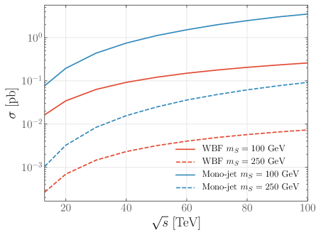
Figure 1: Total cross section values for WBF production of an $S$ pair and two jets through an off-shell Higgs boson at different hadron collider energies (red). We also show the mono-jet signature (blue), mostly originating from gluon fusion. The associated $(H\to SS)Z$ production is suppressed by 3 orders of magnitude compared to WBF production and therefore not included.

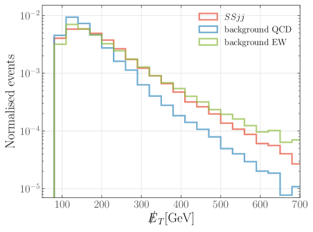
Figure 2: Normalised signal and background distributions of $\not{E}_{T}$ for $m_{S}=100$ GeV and $\lambda=1$ at $100$ TeV FCC. The distributions are obtained with the baseline cuts given in the caption of Tab. 1.

Cuts	$SSjj\;\text{[pb]}\quad$	$Zjj\;\text{[pb]}\quad$	$W^{+}jj\;\text{[pb]}\quad$	$W^{-}jj\;\text{[pb]}\quad$	$Zjj\;\text{EW [pb]}\quad$	$W^{+}jj\;\text{EW [pb]}\quad$	$W^{-}jj\;\text{EW [pb]}\quad$
Baseline	0.0238	10.103	6.6287	3.0501	0.9386	0.5897	0.3833
$\Delta\eta>4.2$	0.0217	6.6052	4.4727	1.9775	0.8325	0.5232	0.3384
$\not{E}_{T}>200$ GeV	0.0080	1.5842	0.7633	0.2666	0.3952	0.1668	0.0940
$m_{jj}>2300$ GeV	0.0041	0.3637	0.2409	0.0637	0.2256	0.1071	0.0594

Table 1: $S$ pair production and background cross sections for WBF at $100$ TeV FCC. The $S$ parameters are set to $m_{S}=100$ GeV and $\lambda=1$, while baseline cuts denote the cuts described in section II.1, but with the relaxed restrictions $\Delta\eta_{jj}>4.0$, $\not{E}_{T}>100$ GeV and $m_{jj}>800$ GeV. QCD corrections will not change these estimates as shown in Ref. Mangano et al. (2017).

Weak boson fusion: Events with $S$ particles generated through weak boson fusion (WBF) are contaminated by $(Z\to{\nu\bar{\nu}})+\text{jets}$ and $(W\to{\ell\nu})+\text{jets}$ processes, with jets originating from either strong or weak interactions. The WBF signal is characterised by a large pseudorapidity $\eta$ separation of high invariant-mass (back-to-back) tagging jets Barger et al. (1991); Rainwater and Zeppenfeld (1999). We cluster jets with the anti-kT algorithm Cacciari et al. (2008) with size $0.4$ following Ref. Sirunyan et al. (2019) and select events with two jets satisfying $p_{T}(j)\geq 50~{}\text{GeV}$ in the region of the hadronic calorimeter parametrised by pseudorapidities $|\eta(j)|<4.7$. Enforcing the WBF signal topology, we require a large pseudorapidity separation of the tagging jets $\lvert\Delta\eta({jj})\rvert>4.0$ at small azimuthal angle $\lvert\Delta\phi_{jj}\rvert<1.5$ while the jets are required to lie in opposite detector hemispheres $\eta(j_{1})\eta(j_{2})<0$. We impose a central jet veto Barger et al. (1995) to suppress QCD-induced signal and background processes by requiring no jets above $p_{T}\geq 30$ GeV between the tagging jets. Given these requirements, top pair production as well as QCD multi-jet production do not constitute dominant backgrounds (see, e.g., Eboli and Zeppenfeld (2000)).

The $(W\to{\ell\nu})+\text{jets}$ contamination is further reduced by vetoing events with isolated leptons. To minimise the impact of jet energy scale uncertainties we further require the azimuthal angle difference between the missing transverse momentum vector $\not{{\bf{p}}}_{T}$ and the transverse momentum of each jet ${\bf{p}}_{T}$ must be greater than $0.5$ rad. This criterion is only applied on jets with $p_{T}>30~{}\text{GeV}$ and is considered sufficient to remove multi-jet production. We will refer to the aforementioned cuts as baseline cuts.

With these cuts the missing energy distribution of signal and background is plotted in Fig. 2. From this we define our search region at sizeable missing energy $\not{E}_{T}=\lvert{\bf{p}}_{T}\rvert>200$ GeV and require the invariant mass of the leading jets, $m_{jj}>2.3$ TeV. For an example with $m_{S}=100~{}\text{GeV}$ the effects of the cuts on signal and background are given explicitly in Tab. 1.

Mono-jet production: An $S$ pair can also be produced with an additional jet, through next-to-leading order (NLO) processes that lead to a single Higgs boson recoiling against QCD radiation. Selection of events is done by requiring a leading jet of $p_{T}>30$ GeV and $\lvert\eta\rvert<2.4$. Radiation of a sub-leading jet with $p_{T}$ above $30$ GeV is allowed, as long as the azimuthal separation between the two jets satisfies $\lvert\Delta\phi(j_{1},j_{2})\rvert<2.5$, to suppress the dijet events. Contamination in such events occurs from processes that yield a $(Z\to{\nu\bar{\nu}})+\text{jet}$ or $(W\to{\ell\nu})+\text{jet}$ final state and is reduced by vetoing any events with isolated electrons or muons. Top and QCD production are subdominant backgrounds (e.g. Aad et al. (2011)). Considering the above as the baseline cuts of our analysis, the missing transverse energy is subsequently restricted to $\not{E}_{T}>150$ GeV and the leading jet transverse momentum to $p_{T}>100$ GeV.

Also for this case we compare signal and background as a function of the missing energy in Fig. 3. The effects of the cuts are demonstrated for the same example as above in Tab. 2.

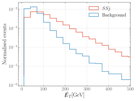
Figure 3: Mono-jet and $S$ pair $\not{E}_{T}$ distribution for $m_{S}=100$ GeV and $\lambda=1$ at $100$ TeV FCC along with combined background using the baseline cuts specified in the caption of Tab. 2.

Cuts	$SSj\;\text{[pb]}\;\;$	$Zj\;\text{[pb]}\;\;$	$W^{-}j\;\text{[pb]}\;\;$	$W^{+}j\;\text{[pb]}$
Baseline	0.9322	15283	17495	19799
$p_{T}(j_{1})>100$ GeV	0.2858	820.54	553.20	670.02
$\not{E}_{T}>150$ GeV	0.1810	298.28	87.381	138.12

Table 2: Cross sections for the production of an $S$ pair and a monojet event at $100$ TeV FCC, with $m_{S}=100$ GeV and $\lambda=1$. Background events are also displayed and for the baseline cuts, no $\not{E}_{T}$ restriction is enforced and a relaxed $p_{T}(j_{1})>30$ GeV is required. $W$ background events are generated with with a minimum lepton cut of $\eta>2.5$ to enhance statistics. Contamination from $t\bar{t}j$ was significantly smaller than the rest of the background processes and is therefore not included. We take into account approximate QCD corrections to the backgrounds via the global $K\simeq 1.6$ factors reported in Mangano et al. (2017).

Lepton Colliders

In analogy to what we have done for the case of hadron colliders we consider for lepton colliders the two main channels for scalar pair production via an off-shell Higgs: associate production and weak boson fusion (see in particular Ruhdorfer et al. (2019) for a recent analysis). For illustration we show an example of the cross section as a function of the centre of mass energy in Fig. 4. The events for the cross sections, as well as the rest of the analysis, are generated with the requirements $p_{T}^{\ell}>10$ GeV, $\lvert\eta(\ell)\rvert<5$ and $\Delta R_{\ell\ell}>0.4$ applied on light leptons $\ell$.

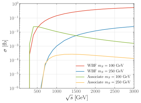
Figure 4: Total cross section values for WBF and associate production of $S$ pair and two leptons at different energies.

Associate production: In contrast to hadron colliders, associate Higgs production at lepton colliders is relevant and comparable to the WBF modes. The signal process $e^{-}e^{+}\rightarrow Z(H\rightarrow SS)$, where the on-shell $Z$ boson decays to a lepton pair, is contaminated by $e^{-}e^{+}\rightarrow\ell^{-}\ell^{+}\nu_{\ell}\bar{\nu}_{\ell}$, where the neutrinos appear as missing energy. The signal is characterised by a smaller pseudorapidity separation between the lepton pair ($\Delta\eta_{\ell\ell}$) and thus the search region is restricted to $\Delta\eta_{\ell\ell}<1.3$. Further distinction from the background is achieved with a cut on the missing energy, $\not{E}_{T}>150$ GeV, and on the missing invariant mass

$$\text{MIM}=\sqrt{\not{p}_{\mu}\not{p}^{\mu}}\geq 200~{}\text{GeV}\,,$$ (5)

where $\not{p}=(\sqrt{s},{\bf{0}})-p_{\ell^{-}}-p_{\ell^{+}}$.

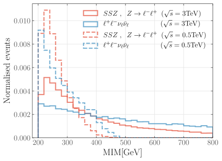
Figure 5: Distributions of MIM for signal and background events with $m_{S}=100$ GeV and $\lambda=1$ at $500$ GeV ILC, where the associate production will be more relevant, as well as $3$ TeV CLIC.

An example of the MIM distribution of signal and backgrounds is shown in Fig. 5. The effects of the cuts are demonstrated in Tab. 3.

Cuts	$SSZ,Z\rightarrow\ell^{+}\ell^{-}\;\text{[fb]}\quad$	$\ell^{+}\ell^{-}\nu_{\ell}\bar{\nu}_{\ell\;}\text{[fb]}$
Generation	0.0236	669.68
$\Delta\eta_{\ell\ell}<1.3$	0.0194	139.64
$\not{E}_{T}>150$ GeV	0.0113	13.786
$\text{MIM}>200$ GeV	0.0113	2.8209
$M_{\ell\ell}<120$ GeV	0.0113	2.3947

Table 3: Cross sections for the associate production of an $S$ pair at lepton colliders with $\sqrt{s}=500$ GeV. Parameters were set to $m_{S}=100$ GeV and $\lambda=1$.

Weak boson fusion: WBF remains the dominant process at centre of mass energies larger than $500$ GeV and it is essential to distinguish it from the associate production. This can be achieved with a cut on the invariant mass of the electron-positron pair. For CLIC at $3$ TeV we use $M_{ee}>2200$ GeV to isolate the signal from contributing backgrounds. The background is further reduced with cuts on the same quantities as in the associate production case. $\Delta\eta_{ee}>6$ is imposed, since WBF results in leptons with large pseudorapidity separation. The search region is restricted to $\not{E}_{T}>80$ GeV and MIM $>200$ GeV. For ILC at $500$ GeV the relaxed restrictions $M_{ee}>120$ GeV and $\Delta\eta_{ee}>2.0$ were used and the rest of the cuts were kept the same. The former cut also removes any signal event produced via associated modes. Examples of the MIM distribution and the cutflow are given in Fig. 6 and Tab. 4.

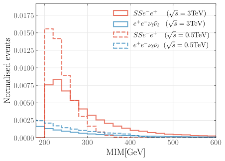
Figure 6: Normalised signal and background distributions of MIM for $m_{S}=100$ GeV and $\lambda=1$ at 500 GeV and 3 TeV lepton colliders produced through WBF. Generation level cuts as in Tab. 4 were used.

Cuts	$SSe^{-}e^{+}\;\;\text{[fb]}\quad$	$e^{+}e^{-}\nu_{\ell}\bar{\nu}_{\ell}\;\text{[fb]}$
Generation	0.5364	43.86
$\text{MIM}>200$ GeV	0.5364	9.257
$\Delta\eta_{ee}>6$	0.4144	1.687
$\not{E}_{T}>80$ GeV	0.2811	1.446
$M_{ee}>2200$ GeV	0.2346	0.468

Table 4: Cross sections for the $S$ pair and background production for WBF at $3$ TeV CLIC, with $m_{S}=100$ GeV and $\lambda=1$. Cuts are enforced at generation level to improve statistics and include a cut on the sum of neutrino’s momenta $\not{E}_{T}^{\nu}>70$ GeV as well as requiring an invariant electron mass of $M_{ee}>1500$ GeV. The latter also removes any event arising from associate production.

Finally, in a WBF topology, where $W$ bosons fuse to produce the Higgs (and neutrinos from the electron and positron), one could use initial state radiation emitted from the colliding electrons or mediating $W$ bosons to trigger the event. In this case, the final state would consist of only a photon and missing energy ($S$ pair and neutrinos) and background contamination would arise from $e^{+}e^{-}\rightarrow\gamma\nu_{e}\bar{\nu}_{e}$. After generating relevant events, we found a significance $N_{S}/\sqrt{N_{B}}=0.0082$, where $N_{S}$ and $N_{B}$ are signal and background events respectively. Hence, this is not an avenue to significantly gain sensitivity to the hidden scalars.

II.2 Indirect Sensitivity: Virtual $S$ imprints

Let us now turn to the indirect measurements, where $S$ is only present in loops (see Noble and Perelstein (2008); Craig et al. (2013); Curtin et al. (2014); Craig et al. (2016); He and Zhu (2017); Kribs et al. (2017); Voigt and Westhoff (2017); Englert and Jaeckel (2019) for previous studies using such observables). Here, we will consider precision observables that are measured at both hadron and lepton colliders. The discussion therefore applies to both types of colliders.

The interactions of Eq. (1) will create corrections to the Higgs and Goldstone boson two-point function. The Higgs potential contained in ${\cal{L}}_{\text{SM}}$ is

$$V(\Phi)=\mu^{2}|\Phi|^{2}+\lambda_{H}|\Phi|^{4}\supset v(\mu^{2}+v^{2}\lambda_{H})H=tH\,.$$ (6)

At leading order this is minimised through conveniently choosing

$$t=v(\mu^{2}+v^{2}\lambda_{H})=0\,.$$ (7)

This choice leads to tadpole diagrams that parametrise the shift of the classical Higgs field value away from the minimum of the Higgs potential as determined by the theory’s free parameters beyond leading order. In general, Higgs boson tadpoles can be removed from higher order corrections by choosing $t=0$ for bare quantities. This introduces a counterterm $\delta t=-\Gamma^{H}(p^{2}=0)$ that corresponds to a renormalisation of the 1-PI Higgs vertex function $\Gamma^{H}(p^{2})$ involving all tadpole diagrams and a correlated Goldstone mass renormalisation (see Denner (1993); Denner and Dittmaier (2019))

$$\delta m_{G}^{2}=-{\delta t\over v}=-{e\over 2m_{W}s_{W}}\delta t$$ (8)

The Goldstone renormalisation will be relevant for the discussion of oblique electroweak corrections in Sec. II.2.4. Note that at one-loop order we can understand $\delta t$ also as

$$\delta v=-{\delta t\over m_{H}^{2}}$$ (9)

which shows that working with the “correct” vacuum expectation value in spontaneously broken gauge theories involves tadpole contributions for vertices that result from setting the Higgs to its vev connected by a zero-momentum propagator. As the trilinear Higgs boson interaction vertex follows from the four-point vertex with one leg set to the Higgs’ vacuum expectation, the tadpole renormalisation together with the Higgs mass and wavefunction renormalisation constants are also relevant for the corrections to Higgs pair production in Sec. II.2.3, see He and Zhu (2017); Kribs et al. (2017); Voigt and Westhoff (2017); Englert and Jaeckel (2019).

II.2.1 Higgs coupling modifications

Measurements of Higgs boson rates are typically reported using the narrow width approximation owing to the narrowness of the Higgs boson $\Gamma_{H}/m_{H}\simeq{\cal{O}}({10^{-5}})$. Signal strengths $\mu$ are then obtained by comparing observations against the SM expectation

$$\mu={\sigma(H)\times{\text{BR}}\over[\sigma(H)\times{\text{BR}}]_{\text{SM}}}$$ (10)

where $\sigma(H)$, BR represent particular Higgs boson production and decay branching modes. For the model given in Eq. (1) when $m_{S}>m_{H}/2$ no non-SM Higgs decay channel are present. In this case, all modifications away from the SM will be due to virtual $S$ effects (see Ref. Craig et al. (2013, 2016); Englert and Jaeckel (2019) for earlier analyses).

The Higgs wave function and mass squared renormalisation constants in the on-shell scheme are given by

$$\delta Z_{H}=-{\lambda^{2}\over 8\pi^{2}}{2m_{W}s_{W}\over e}\hbox{Re}{\partial B_{0}(q^{2},m_{S}^{2},m_{S}^{2})\over\partial q^{2}}\bigg{|}_{q^{2}=m_{H}^{2}}\,,$$ (11)

and

$$\delta m_{H}^{2}={\lambda^{2}\over 8\pi^{2}}{4m_{W}^{2}s_{W}^{2}\over e^{2}}\hbox{Re}B_{0}(m_{H}^{2},m_{S}^{2},m_{S}^{2})\\ +{\lambda\over 16\pi^{2}}\hbox{Re}A_{0}(m_{S}^{2})$$ (12)

with Passarino-Veltman Passarino and Veltman (1979) functions $A_{0},B_{0}$ which are given in $D$-dimensional regularisation in e.g. Ref. Denner (1993) (see also Scharf and Tausk (1994); Martin and Robertson (2006)). The $D\to 4$ divergent pieces of the $B_{0}$ are momentum-independent. This renders $\delta Z_{H}$ finite for the scenario in this paper and at the given order in perturbation theory. Any single Higgs production process or partial decay width $\Gamma_{i}$ will then obtain an $S$-correction

$${\sigma(H)\over[\sigma(H)]_{\text{SM}}}={\Gamma_{i}\over[\Gamma_{i}]_{\text{SM}}}=1+\delta Z_{H}$$ (13)

which leads to (see also Englert and McCullough (2013); Craig et al. (2013, 2015))

$$\mu={\sigma(H)\times{\text{BR}}\over[\sigma(H)\times{\text{BR}}]_{\text{SM}}}=1+\delta Z_{H}\,.$$ (14)

Constraints on the Higgs signal strength Englert et al. (2017) can therefore be treated analogously to Higgs portal models with a dark vacuum expectation value leading to Higgs coupling modifications proportional to a characteristic Higgs mixing angle, which can be identified with $\delta Z_{H}$.

Note that given that the Higgs coupling modifications are uniform, all relevant information in the comparison against the SM is contained in the total cross section and, consequently, in the signal strength constraint.

II.2.2 Off-Shell Higgs boson probes

A channel that received considerable interest recently in the context of Higgs coupling studies at hadron colliders is the so-called off-shell measurement of $p(g)p(g)\to H\to ZZ\to 4~{}\text{leptons}$. Due to unitarity cancellations in the absorptive parts of the amplitude linked to $t\bar{t}\to ZZ$ scattering, the Higgs contributions are non-decoupling for energies above the Higgs resonance Kauer and Passarino (2012). Correlating Higgs off-shell with on-shell $H\to ZZ$ measurements (Eq. (10)) can then be interpreted as an indirect measurement of the Higgs width Caola and Melnikov (2013); Englert and Spannowsky (2014) under assumptions of how these different kinematic regions are connected Englert et al. (2015).

In the scenario of Eq. (1) at ${\cal{O}}(\lambda^{2})$, the $gg\to ZZ$ continuum is unchanged while the Higgs contributions receive corrections from the scalar $S$. The modification of the $s$-channel Higgs exchange amplitude ${\cal{M}}$ is given by

$${{\cal{M}}\over{\cal{M}}_{\text{SM}}}-1=-{\lambda^{2}m_{W}^{2}s_{W}^{2}\over 8\pi^{3}\alpha(s-m_{H}^{2})}\\ \times\left(B_{0}(s,m_{S}^{2},m_{S}^{2})-\hbox{Re}B_{0}(m_{H}^{2},m_{S}^{2},m_{S}^{2})\right)\,.$$ (15)

Note that the right hand side vanishes when we take the limit $s\to m_{H}^{2}$ as expected from the cancellation of vertex and propagator renormalisations when we do not include the finite lifetime of the Higgs boson with an ad-hoc Breit-Wigner distribution. Including the modification of the total Higgs decay width according to Eq. (13) results again in Eq. (14) upon expansion.

This channel only shows limited sensitivity as can be seen from Fig. 7. As can be expected from the discussion of Ref. Englert et al. (2019), the corrections of Eq. (15) are small even before interfering with the SM $gg\to ZZ$ continuum amplitude. Even for extrapolations to 30/ab at a 100 TeV FCC-hh that are typically discussed as design targets for such a machine Abada et al. (2019a, b, c, d), we do not obtain constraints in this channel that are robust in the sense of perturbative unitarity (see below).

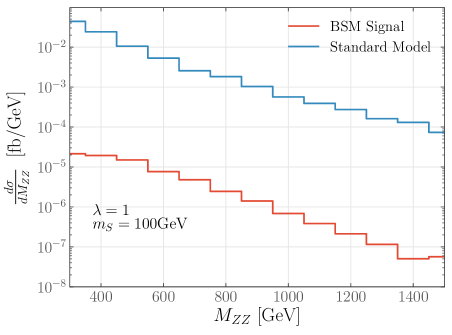
Figure 7: Differential cross sections for $gg\rightarrow ZZ$ at $100$ TeV FCC, indicating that corrections originating from $S$ to the Higgs contribution of $pp\rightarrow 4\ell$ are negligible.

II.2.3 Higgs Pair Production

Virtual $S$-loops also modify Higgs pair production Noble and Perelstein (2008); Curtin et al. (2014); He and Zhu (2017); Voigt and Westhoff (2017); Englert and Jaeckel (2019). As the trilinear Higgs boson interaction vertex follows from the four-point vertex with one leg set to the Higgs’ vacuum expectation value, the 3-point Higgs function is still a function of the tadpole renormalisation constant $\delta t$ even when we remove tadpoles throughout the calculation by choosing a tadpole renormalisation

$$\delta t=-{\lambda\over 8\pi^{2}}{2m_{W}s_{W}\over e}\hbox{Re}A_{0}(m_{S}^{2})\,.$$ (16)

The amplitude for the relevant $HH$ production (i.e. weak boson fusion $e^{+}e^{-}\to HH\nu_{e}\bar{\nu}_{e}$ at high-energy lepton colliders and $gg\to HH$ at hadron colliders) is then obtained from expanding the transition probability

$$|{\cal{M}}|^{2}=|{\cal{M}}_{\text{SM}}|^{2}+2\text{Re}\left({\cal{M}}_{\text{SM}}{\cal{M}}^{\ast}_{{\lambda}}\right)\,,$$ (17)

where SM/$\lambda$ refer to the leading order and next-to-leading order contributions $\sim\lambda$, respectively. We will consider the next-to-leading correction in the following, see Englert and Jaeckel (2019).

II.2.4 Oblique Corrections

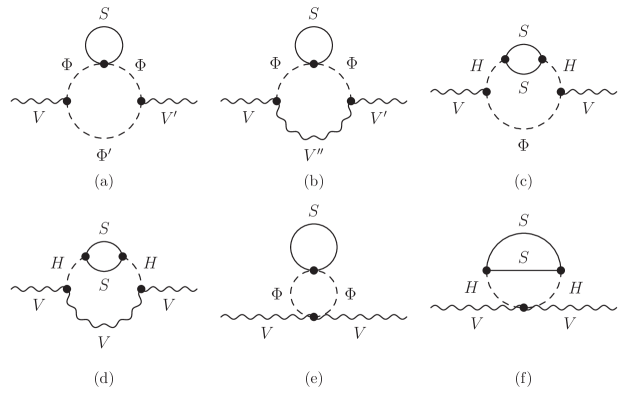
Figure 8: Representative two-loop Feynman diagram topologies of the electroweak boson polarisation functions for boson $V$ that give rise to the electroweak oblique corrections $S,T,U\sim\lambda,\lambda^{2}$. $\Phi,\Phi^{\prime}$ denote all possible Higgs and Goldstone boson insertions. $V,V^{\prime},V^{\prime\prime}=W,Z,A$ label all allowed SM vector boson insertions.

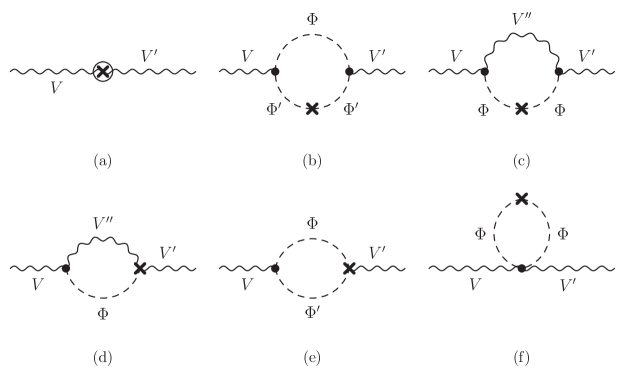
Figure 9: Representative two-loop Feynman diagram counter term topologies of the electroweak boson polarisation functions similar to Fig. 8. The first diagram represents two-loop renormalisation constants that are not obtained from one-loop inserted one-loop renormalisation constants. Note that $\Phi\Phi^{\prime}V^{\prime\prime}$ vertex counterterms are suppressed.

The Peskin-Takeuchi $S,T,U$ parameters Peskin and Takeuchi (1990) follow from an investigation of polarisation functions $\Pi_{VV^{\prime}}$

$$\parbox{99.58464pt}{\vspace{0.15cm}\includegraphics[width=99.58464pt]{twopoint.pdf}}\sim\Pi_{VV^{\prime}}^{\mu\nu}(p^{2})\\ =(p^{2}-m_{V}^{2})\delta_{VV^{\prime}}+\Pi_{VV^{\prime}}(p^{2})\left(g^{\mu\nu}-{p^{\mu}p^{\nu}\over p^{2}}\right)\\ +B_{VV^{\prime}}(p^{2}){p^{\mu}p^{\nu}\over p^{2}}\,,$$ (18)

and their transverse parts in particular. The so-called oblique corrections are then given by (see also Golden and Randall (1991); Holdom and Terning (1990); Altarelli and Barbieri (1991); Grinstein and Wise (1991); Peskin and Takeuchi (1992); Altarelli et al. (1992); Burgess et al. (1994); Barbieri et al. (2004))

$$\begin{split}S&={4s_{W}^{2}c_{W}^{2}\over\alpha}\left(\frac{\Pi_{ZZ}(m_{Z}^{2})-\Pi_{ZZ}(0)}{m_{Z}^{2}}-{c_{W}^{2}-s_{W}^{2}\over c_{W}s_{W}}{\Pi_{AZ}(m_{Z}^{2})-\Pi_{AZ}(0)\over m_{Z}^{2}}-{\Pi_{AA}(m_{Z}^{2})\over m_{Z}^{2}}\right)\,,\\ T&={1\over\alpha}\left({\Pi_{WW}(0)\over m_{W}^{2}}-{\Pi_{ZZ}(0)\over m_{Z}^{2}}-{2s_{W}\over c_{W}}{\Pi_{AZ}(0)\over m_{Z}^{2}}\right)\,,\\ U&={4s_{W}^{2}\over\alpha}\left({\Pi_{WW}(m_{W}^{2})-\Pi_{WW}(0)\over m_{W}^{2}}-c_{W}^{2}{\Pi_{ZZ}(m_{Z}^{2})-\Pi_{ZZ}(0)\over m_{Z}^{2}}\right.-2s_{W}c_{W}{\Pi_{AZ}(m_{Z}^{2})-\Pi_{AZ}(0)\over m_{Z}^{2}}-\left.s_{W}^{2}{\Pi_{AA}(m_{Z}^{2})\over m_{Z}^{2}}\right)\,,\end{split}$$ (19)

where $c_{W},s_{W}$ are the cosine and sine of the Weinberg angle, respectively. $S,T,U$ parametrise the leading modifications of gauge boson interactions due to presence of new physics affecting their propagation, i.e. they capture correlated modifications away from the SM expectation of electroweak four-fermion scattering processes. As the new scalar only couples to the Higgs boson and is protected by the unbroken ${\mathbb{Z}}_{2}$-symmetry, contributions to $S,T,U$ do only arise at two-loop order. The relevant diagrams and counterterms are given in Fig. 8 and 9, respectively.

In the definition of Eq. (19) we have already exploited the Ward identity $\Pi_{AA}(0)=0$ which means that we will work with on-shell renormalised quantities in the following. For instance, for our scalar $S$ insertions we obtain before renormalisation in $D$-dimensional regularisation and using Feynman gauge, Fig. 8 (a),(b),(e),

$$\Pi^{0}_{AA}(0)=-{\alpha(D-4)(D-2)\over 256\pi^{3}m_{W}^{2}}\lambda A_{0}(m_{S}^{2})A_{0}(m_{W}^{2})$$ (20)

where $A_{0}$ is the standard function one-loop function (expanding $D=4-\epsilon<4$)

$$A_{0}(x)=x\bigg{[}{2\over\epsilon}-\gamma_{E}-\log{x\over 4\pi\mu^{2}}+1+\\ {\epsilon\over 4}\big{(}(-\gamma_{E}-\log{x\over\mu^{2}}+1)^{2}+1+{\pi^{2}\over 6}\bigg{)}\bigg{]}\,.$$ (21)

This yields

$$\Pi^{0}_{AA}(0)={\alpha\lambda m_{S}^{2}\over 32\pi^{3}}\bigg{(}{1\over\epsilon}-\gamma_{E}+\log\left({m_{S}m_{W}\over 4\pi\mu^{2}}\right)-{1\over 2}\bigg{)}\\ +{\cal{O}}(\epsilon)\,.$$ (22)

This cancels identically against the renormalised Goldstone contribution

$$\delta\Pi_{AA}(0)=-{\alpha(D-4)(D-2)\over 32\pi^{2}m_{W}^{2}}{e\,\delta t\over m_{W}s_{W}}A_{0}(m_{W}^{2})$$ (23)

with the one-loop tadpole renormalisation $\delta t$ given in Eq. (16).

We compute the oblique corrections using a combination of FeynCalc Mertig et al. (1991); Shtabovenko et al. (2016), FeynArts Hahn (2001), LoopTools Hahn and Perez-Victoria (1999); Hahn (2000), Tarcer Mertig and Scharf (1998) and we perform analytical checks to ensure UV finiteness. Full numerical results are then obtained by employing Tsil Martin and Robertson (2006), which is based on Ref. Tarasov (1997) (see also Weiglein et al. (1994)). In Fig. 10 the results are shown as a function of the scalar mass.

For the oblique parameters, we note that the $U$ parameter is suppressed by an order of magnitude compared to $S,T$. This can be seen in Fig. 10. This is consistent with the fact that $U$ is not sourced by dimension 6 effective operators. We therefore employ the $U=0$ projections of Ref. Baak et al. (2014) for the GFitter LHC 300/fb and ILC/GigaZ options.

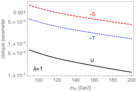
Figure 10: Oblique parameter values for different scalar masses and $\lambda=1$.

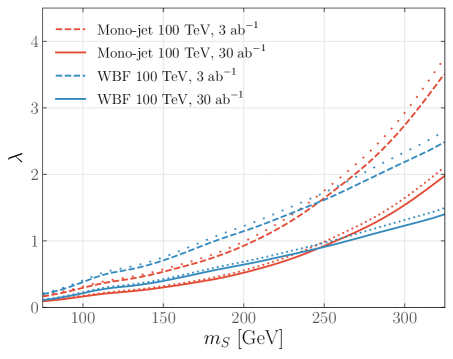
Figure 11: (a) 68% exclusion regions for FCC at $3\;\text{ab}^{-1}$ and $30\;\text{ab}^{-1}$ integrated luminosities, as identified with $N_{S}/\sqrt{N_{S}+N_{B}}=1$. Dotted and loosely dotted lines correspond to a $30\%$ increment of the background for the $3\;\text{ab}^{-1}$ and $30\;\text{ab}^{-1}$ cases respectively. (b) 68% exclusion regions for ILC at $2\;\text{ab}^{-1}$ luminosity and 3 TeV CLIC at $3\;\text{ab}^{-1}$.

III Power meets Precision: Expected Collider Sensitivity

Before we turn to the discussion of the expected sensitivity to the parameters $\lambda,m_{S}$ it is instructive to consider the perturbative unitarity constraints on $\lambda$. Forward $SH\to SH$ scattering in the high energy limit $s=(p_{S}+p_{H})^{2}\gg m_{H},m_{S}$ and the perturbative constraint on the zeroth partial wave (see e.g. Dawson et al. (2019))

$$\text{Re}\,a_{0}(SH\to SH)\leq{1\over 2}$$ (24)

yields straightforwardly $\lambda\lesssim 4\pi$. We find that this limit is quickly approached at around $\sqrt{s}\simeq 3.5~{}\text{TeV}$ for the mass range $m_{Z}<m_{S}\lesssim 300~{}\text{GeV}$ that we consider in this work. It is worthwhile to note that this perturbativity constraint is weaker than the electroweak stability bounds, see Curtin et al. (2014), which limit $|\lambda|\lesssim 1$.

The direct cross section measurements are summarised in Fig. 11. After all cuts have been applied, the 68% exclusion regions are obtained by requiring $N_{S}/\sqrt{N_{S}+N_{B}}=1$, where $N_{S}$ and $N_{B}$ are signal and background events, respectively. The analysis was employed for $100$ TeV FCC for integrated luminosities of $3~{}\text{ab}^{-1}$ and $30~{}\text{ab}^{-1}$, with WBF being more sensitive at masses larger than $m_{S}=250$ GeV compared to mono-jet production. Exclusion regions are studied for $500$ GeV ILC at $2~{}\text{ab}^{-1}$, which will be reached at later stages of the experiment according to Ref. Aihara et al. (2019) and associate production is the most sensitive process in this case. In contrast, WBF is the only significant process at the higher energies of $3$ TeV at $3~{}\text{ab}^{-1}$ that can be reached by CLIC.

We now turn to the expected precision of Higgs signal strength measurements at different colliders.

Projections of single Higgs measurements in the context of singlet extensions have been provided in, e.g., Ref. Klute et al. (2013). We find that the projected global constraints on universal Higgs mixing for 240 GeV lepton colliders are in good agreement with constraints that we obtain from a projection of $e^{+}e^{-}\to HZ$ alone. Based on this we focus on this single measurement to constrain universal Higgs coupling modifications for all types of colliders.

The fit of Ref. Klute et al. (2013) gives

$$\text{LHC}: \quad\mu=[0.96,1.03]$$ (25a)

for LHC projections. A dedicated recent analysis of Higgs coupling measurements at lepton colliders de Blas et al. (2019) finds fractional signal strength uncertainty of

$$\text{ILC-250}: \quad{\delta\mu\over\mu}=0.29\%\,,$$ (25b)

$$\text{CLIC-380}: \quad{\delta\mu\over\mu}=0.44\%\,,$$ (25c)

$$\text{FCC-ee(240)}: \quad{\delta\mu\over\mu}=0.2\%\,.$$ (25d)

At a future FCC-hh option we can expect Abada et al. (2019b)

$$\text{FCC-hh}: \quad{\delta\mu\over\mu}=1.22-1.88\%\,,$$ (25e)

depending on the Higgs decay channel. The results for the different experiments are shown in Fig. 12.

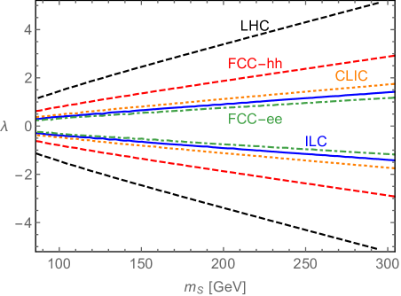
Figure 12: Higgs signal strength measurements at different colliders interpreted in the singlet off-shell model. The limits are based on the uncertainties stated in Eqs. (25a)-(25e).

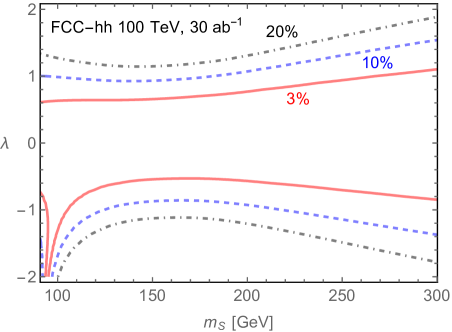
Figure 13: Sensitivity of di-Higgs production at the FCC-hh (30/ab) to the symmetric off-shell Higgs portal based on an inclusive $\kappa_{\lambda}$ measurement. The different lines refer to the expected accuracy of $\kappa_{\lambda}$, where 3% is the 68% confidence level reported in Ref. Contino et al. (2017). The di-Higgs results for CLIC are qualitatively identical and given in Fig. 15(b).

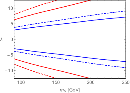
Figure 14: (a) LHC 300/fb (red) and ILC/GigaZ (blue) Baer et al. (2013) $S,T$ constraints at 68% (solid) and 95% confidence level (dashed) as provided by GFitter Baak et al. (2014) for $U=0$ when considered in the parameter space of the portal model at two-loop level.

For measurements of the Higgs self-coupling, a recent CMS projection gives 68% and 95% confidence level projections $\kappa^{\text{68\%}}_{\lambda_{\text{SM}}}={\lambda^{\text{68\%}}_{\text{SM}}/\lambda_{\text{SM}}}=[0.35,1.9]$, and $\kappa^{\text{95\%}}_{\lambda_{\text{SM}}}={\lambda^{\text{95\%}}_{\text{SM}}/\lambda_{\text{SM}}}=[-0.18,3.6]$ (see Ref.  Sirunyan et al. (2018)), where $\lambda_{\text{SM}}$ is the SM Higgs self-coupling. Note that these limits are not much further than a factor of order two away from the perturbative limits of forward $HH$ scattering. While these constraints are perturbatively meaningful they do not suggest large sensitivity to weakly coupled, non-resonant Higgs sector extensions. This is owed to the fact of a relatively small inclusive di-Higgs cross section of about 32 fb at the LHC Dawson et al. (1998); Frederix et al. (2014); de Florian and Mazzitelli (2015); de Florian et al. (2016); Borowka et al. (2016a, b); Heinrich et al. (2017); Grazzini et al. (2018); De Florian and Mazzitelli (2018); Baglio et al. (2019). Enhancing sensitivity to Higgs pair production is a key motivation for pushing the energy frontier beyond the LHC.

Turning to a future hadron collider with 100 TeV centre-of-mass energy, the measurement of the Higgs self-coupling is expected to reach up to $3-6\%$ precision with regard to the machine’s and the estimated detector capability Contino et al. (2017); Banerjee et al. (2018, 2019). Following Englert and Jaeckel (2019) and interpreting inclusive Higgs self-coupling measurements (i.e. the associated cross section difference) of $\kappa_{\lambda}$ along the lines of $S$-induced corrections, we obtain the results of Fig. 13. We note that 3% sensitivity is below the currently understood theoretical limitations of $\sim 10\%$ Alison et al. (2019), which will saturate the uncertainty of the self-coupling measurement extraction unless theoretical improvements become available. For comparison we therefore include re-interpretations of $\delta\kappa_{\lambda_{\text{{SM}}}}/\kappa_{\lambda_{\text{{SM}}}}=10\%,20\%$ in Fig. 13. The behaviour of self-coupling measurements in the WBF channel at lepton colliders is qualitatively identical and we will discuss them in the next section.

Let us now turn to the oblique parameters. For $S$ and $T$ the correlation matrices, central values and uncertainties for the LHC and GigaZ are given by Baak et al. (2014)

$$\text{LHC}: ~{}\rho=\left(\begin{matrix}1&0.96\\ 0.96&1\end{matrix}\right) (\Delta S,\Delta T)=(0.086,0.064)\,,$$ (26)

$$\text{GigaZ}: ~{}\rho=\left(\begin{matrix}1&0.91\\ 0.91&1\end{matrix}\right) (\Delta S,\Delta T)=(0.018,0.023)\,.$$ (27)

From these we can obtain a $\chi^{2}$ through the inverse error-multiplied correlation matrix, which is translated to our Higgs portal parameters in Fig. 14. As can be seen, the constraints that can be expected at the LHC in the near future are not competitive with the indirect constraints from on-shell Higgs measurements. GigaZ improves this dramatically, however, the sensitivity is still too low for the two-loop contributions to compete with Higgs measurements at Higgs factories such as ILC, CLIC and FCC-ee. An improvement in the electroweak measurement by $\sim 30$ would be necessary to become competitive. While this suggests that electroweak precision measurements are unlikely to play a fundamental role in constraining the parameter space of the outlined off-shell Higgs portal, the fact that the required improvement is much smaller than the naive loop factor suppression $\sim 16\pi^{2}$ highlights the generic relevance of electroweak precision constraints for general future BSM investigations.

(a)

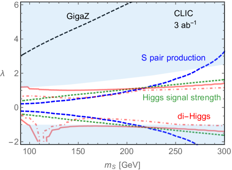
(b)

Figure 15: Comparison of the (a) FCC-hh and (b) CLIC at 3 TeV best case sensitivities. The dashed blue line refers to WBF to the sensitivity of $S$ pair production, while the dotted green line reflects the expected Higgs signal strength constraints. For comparison we include the GigaZ extrapolation of the sensitivity via oblique corrections as a black dashed line. The projected self-coupling extraction are shown in red. For the 3 TeV CLIC the $5\%$- and $10\%$-level are included as dash-dotted and solid lines, respectively. For the Higgs signal strength here we use the 3 TeV value $\delta\mu/\mu=0.39\%$ according to Ref. de Blas et al. (2019). The shaded region is excluded from stability considerations Curtin et al. (2014) and assumes no additional BSM matter content beyond the singlet scalar.

IV Discussion and Conclusions

We can now turn to a comparison of the expected sensitivity to this difficult to access new physics scenario. An overview for the examples of FCC-hh and CLIC is shown in Fig. 15.

Amongst the indirect, loop-induced production processes di-Higgs production provides the best sensitivity, owing to the fact the $gg\to hh$ is largely driven by top-related threshold effects that are particularly sensitive to modifications of the trilinear Higgs coupling as predicted in the model at the expected self-coupling extraction precision. While for FCC-hh measurements of the Higgs signal strength cannot compete, the situation is different for lepton colliders such as CLIC, Fig. 15. For CLIC the Higgs self-coupling and the signal-strength measurements are comparable over a wide mass range. Off-shell $gg\to H\to ZZ$ production is essentially blind to this scenario due to gauge-related cancellations in the reasonable $\lambda$ range (cf. Fig. 7).

The electroweak precision constraint that we present here for the first time originate from the a priori most precise observables that can be obtained at the discussed colliders (see also the related Ref. Chen and Freitas (2020) for recent theoretical developments). Unfortunately, due to the fact that the contributions from the new scalar only arise at two-loops, they will only start to become sensitive to $S$-induced modification if the expected sensitivity is improved by an order of magnitude .

At masses $\lesssim(200-250)\,{\rm GeV}$ the best sensitivity arises in $H\to SS$ off-shell missing energy searches. Together with Higgs-self-coupling measurements and, in the case of CLIC, the Higgs signal-strength measurements they are therefore the most promising avenues to discover or constrain the presence of weakly coupled scalars as expressed in Eq. (1). If even more precise Higgs signal-strength measurements, as indicated by the FCC-ee projections, are achieved this could allow us to reach a similar sensitivity as the combined direct production and indirect di-Higgs probes at FCC-hh, as can be seen from Fig. 12.

However, the importance of the different analyses (and the different collider concepts as a consequence), does crucially rest on the expected precision and control of the different final states measurements. For example, a 3% accuracy of the Higgs self-coupling at a FCC-hh as detailed in Ref. Contino et al. (2017) provides favourable constraints at larger masses in the light of expected direct sensitivity. While this precision seems attainable from an experimental perspective (b-tagging, fake rates, etc.), it relies on an improvement of the theoretical uncertainty budget. Relaxing the self-coupling extraction to $\sim 10\%$, direct off-shell $H\to SS$ limits start to dominate the sensitivity. As noted before, these do also suffer from small signal-over-background ratios and crucially depend on the understanding of the backgrounds. In both instances, data-driven techniques as considered in Aad et al. (2016); Aaboud et al. (2018, 2020) could help to control uncertainties when perturbative improvements are out of reach. However, the combination of both channels capture the induced modifications over a wide range of masses. At future lepton colliders, we find a similar picture. The extrapolations of Charles et al. (2018); de Blas et al. (2018) suggest that the Higgs self-coupling can be determined at 3 TeV in the WBF at the 5-10% level. Recast to the singlet scenario, we see that the di-Higgs production provides a slightly enhanced sensitivity at larger masses compared to direct and signal strength measurements. We note that this sensitivity crucially relies on the expected self-coupling precision. For instance, the slightly more conservative estimate of 22% reported in Ref. Abramowicz et al. (2017) is already too low to be competitive with the expected Higgs signal strength constraints.

While the scenario that we consider in this work is, by construction, difficult to observe, our results do suggest that the discovery potential of the FCC-hh concept can be similar or larger than that of lepton colliders in case systematics are under control. While this is not a surprise for heavy strongly-coupled physics such as SUSY, the combination of energy coverage and statistics, makes a naively sensitivity-limited hadron-hadron machine also an excellent tool to constrain weakly coupled electroweak extensions. In this sense, when power is applied in a controlled way to the symmetric Higgs portal, it will likely beat precision.

Acknowledgements — We thank Federica Fabbri and Jay Howarth for helpful discussions. C.E. is supported by the UK Science and Technology Facilities Council (STFC) under grant ST/P000746/1 and by the IPPP Associateship Scheme. J.J. would like to thank the IPPP for hospitality and gratefully acknowledges support under the DIVA fellowship program of the IPPP. This work was completed while J.J. was at the Munich Institute for Astro- and Particle Physics (MIAPP) which is funded by the Deutsche Forschungsgemeinschaft (DFG, German Research Foundation) under Germany’s Excellence Strategy – EXC-2094 – 390783311. M.S. is supported by the STFC under grant ST/P001246/1. P.S. is supported by an STFC studentship under grant ST/T506102/1.

References

- Abada et al. (2019a) A. Abada et al. (FCC), Eur. Phys. J. ST 228, 261 (2019a).
- Abada et al. (2019b) A. Abada et al. (FCC), Eur. Phys. J. ST 228, 755 (2019b).
- Abada et al. (2019c) A. Abada et al. (FCC), Eur. Phys. J. C79, 474 (2019c).
- Erler et al. (2000) J. Erler, S. Heinemeyer, W. Hollik, G. Weiglein, and P. M. Zerwas, Phys. Lett. B486, 125 (2000), [,1389(2000)], eprint hep-ph/0005024.
- Erler and Heinemeyer (2001) J. Erler and S. Heinemeyer, in Proceedings, 5th International Symposium on Radiative Corrections - RADCOR 2000 (2001), eprint hep-ph/0102083, URL http://www.slac.stanford.edu/econf/C000911/.
- Baer et al. (2013) H. Baer, T. Barklow, K. Fujii, Y. Gao, A. Hoang, S. Kanemura, J. List, H. E. Logan, A. Nomerotski, M. Perelstein, et al. (2013), eprint 1306.6352.
- Binoth and van der Bij (1997) T. Binoth and J. J. van der Bij, Z. Phys. C75, 17 (1997), eprint hep-ph/9608245.
- Schabinger and Wells (2005) R. M. Schabinger and J. D. Wells, Phys. Rev. D72, 093007 (2005), eprint hep-ph/0509209.
- Patt and Wilczek (2006) B. Patt and F. Wilczek (2006), eprint hep-ph/0605188.
- Ahlers et al. (2008) M. Ahlers, J. Jaeckel, J. Redondo, and A. Ringwald, Phys. Rev. D78, 075005 (2008), eprint 0807.4143.
- Batell et al. (2009) B. Batell, M. Pospelov, and A. Ritz, Phys. Rev. D79, 115008 (2009), eprint 0903.0363.
- Englert et al. (2011) C. Englert, T. Plehn, D. Zerwas, and P. M. Zerwas, Phys. Lett. B703, 298 (2011), eprint 1106.3097.
- Ellis et al. (2019) R. K. Ellis et al. (2019), eprint 1910.11775.
- Silveira and Zee (1985) V. Silveira and A. Zee, Phys. Lett. 161B, 136 (1985).
- McDonald (2002) J. McDonald, Phys. Rev. Lett. 88, 091304 (2002), eprint hep-ph/0106249.
- Davoudiasl et al. (2005a) H. Davoudiasl, R. Kitano, T. Li, and H. Murayama, Phys. Lett. B609, 117 (2005a), eprint hep-ph/0405097.
- Barger et al. (2008) V. Barger, P. Langacker, M. McCaskey, M. J. Ramsey-Musolf, and G. Shaughnessy, Phys. Rev. D77, 035005 (2008), eprint 0706.4311.
- Batell et al. (2011) B. Batell, J. Pradler, and M. Spannowsky, JHEP 08, 038 (2011), eprint 1105.1781.
- Khoze et al. (2014) V. V. Khoze, C. McCabe, and G. Ro, JHEP 08, 026 (2014), eprint 1403.4953.
- Feng et al. (2015) L. Feng, S. Profumo, and L. Ubaldi, JHEP 03, 045 (2015), eprint 1412.1105.
- Athron et al. (2018) P. Athron, J. M. Cornell, F. Kahlhoefer, J. Mckay, P. Scott, and S. Wild, Eur. Phys. J. C78, 830 (2018), eprint 1806.11281.
- Arcadi et al. (2019) G. Arcadi, A. Djouadi, and M. Raidal (2019), eprint 1903.03616.
- Hardy (2018) E. Hardy, JHEP 06, 043 (2018), eprint 1804.06783.
- Bernal et al. (2019) N. Bernal, C. Cosme, T. Tenkanen, and V. Vaskonen, Eur. Phys. J. C79, 30 (2019), eprint 1806.11122.
- Alonso-Álvarez et al. (2019) G. Alonso-Álvarez, J. Gehrlein, J. Jaeckel, and S. Schenk (2019), eprint 1906.00969.
- Noble and Perelstein (2008) A. Noble and M. Perelstein, Phys. Rev. D78, 063518 (2008), eprint 0711.3018.
- Craig et al. (2013) N. Craig, C. Englert, and M. McCullough, Phys. Rev. Lett. 111, 121803 (2013), eprint 1305.5251.
- Kribs et al. (2017) G. D. Kribs, A. Maier, H. Rzehak, M. Spannowsky, and P. Waite, Phys. Rev. D95, 093004 (2017), eprint 1702.07678.
- Curtin et al. (2014) D. Curtin, P. Meade, and C.-T. Yu, JHEP 11, 127 (2014), eprint 1409.0005.
- Craig et al. (2016) N. Craig, H. K. Lou, M. McCullough, and A. Thalapillil, JHEP 02, 127 (2016), eprint 1412.0258.
- Ruhdorfer et al. (2019) M. Ruhdorfer, E. Salvioni, and A. Weiler (2019), eprint 1910.04170.
- He and Zhu (2017) S.-P. He and S.-h. Zhu, Phys. Lett. B764, 31 (2017), eprint 1607.04497.
- Voigt and Westhoff (2017) A. Voigt and S. Westhoff, JHEP 11, 009 (2017), eprint 1708.01614.
- Englert and Jaeckel (2019) C. Englert and J. Jaeckel, Phys. Rev. D100, 095017 (2019), eprint 1908.10615.
- Eboli and Zeppenfeld (2000) O. J. P. Eboli and D. Zeppenfeld, Phys. Lett. B495, 147 (2000), eprint hep-ph/0009158.
- Godbole et al. (2003) R. M. Godbole, M. Guchait, K. Mazumdar, S. Moretti, and D. P. Roy, Phys. Lett. B571, 184 (2003), eprint hep-ph/0304137.
- Davoudiasl et al. (2005b) H. Davoudiasl, T. Han, and H. E. Logan, Phys. Rev. D71, 115007 (2005b), eprint hep-ph/0412269.
- Feng et al. (2006) J. L. Feng, S. Su, and F. Takayama, Phys. Rev. Lett. 96, 151802 (2006), eprint hep-ph/0503117.
- Englert et al. (2012) C. Englert, J. Jaeckel, E. Re, and M. Spannowsky, Phys. Rev. D85, 035008 (2012), eprint 1111.1719.
- Christensen and Duhr (2009) N. D. Christensen and C. Duhr, Comput. Phys. Commun. 180, 1614 (2009), eprint 0806.4194.
- Alloul et al. (2014) A. Alloul, N. D. Christensen, C. Degrande, C. Duhr, and B. Fuks, Comput. Phys. Commun. 185, 2250 (2014), eprint 1310.1921.
- Degrande (2015) C. Degrande, Comput. Phys. Commun. 197, 239 (2015), eprint 1406.3030.
- Alwall et al. (2011) J. Alwall, M. Herquet, F. Maltoni, O. Mattelaer, and T. Stelzer, JHEP 06, 128 (2011), eprint 1106.0522.
- de Aquino et al. (2012) P. de Aquino, W. Link, F. Maltoni, O. Mattelaer, and T. Stelzer, Comput. Phys. Commun. 183, 2254 (2012), eprint 1108.2041.
- Alwall et al. (2014) J. Alwall, R. Frederix, S. Frixione, V. Hirschi, F. Maltoni, O. Mattelaer, H. S. Shao, T. Stelzer, P. Torrielli, and M. Zaro, JHEP 07, 079 (2014), eprint 1405.0301.
- Sjöstrand et al. (2015) T. Sjöstrand, S. Ask, J. R. Christiansen, R. Corke, N. Desai, P. Ilten, S. Mrenna, S. Prestel, C. O. Rasmussen, and P. Z. Skands, Comput. Phys. Commun. 191, 159 (2015), eprint 1410.3012.
- Dobbs and Hansen (2001) M. Dobbs and J. B. Hansen, Comput. Phys. Commun. 134, 41 (2001).
- Buckley et al. (2013) A. Buckley, J. Butterworth, L. Lonnblad, D. Grellscheid, H. Hoeth, J. Monk, H. Schulz, and F. Siegert, Comput. Phys. Commun. 184, 2803 (2013), eprint 1003.0694.
- Mangano et al. (2017) M. L. Mangano et al., CERN Yellow Rep. pp. 1–254 (2017), eprint 1607.01831.
- Barger et al. (1991) V. D. Barger, K.-m. Cheung, T. Han, J. Ohnemus, and D. Zeppenfeld, Phys. Rev. D44, 1426 (1991).
- Rainwater and Zeppenfeld (1999) D. L. Rainwater and D. Zeppenfeld, Phys. Rev. D60, 113004 (1999), [Erratum: Phys. Rev.D61,099901(2000)], eprint hep-ph/9906218.
- Cacciari et al. (2008) M. Cacciari, G. P. Salam, and G. Soyez, JHEP 04, 063 (2008), eprint 0802.1189.
- Sirunyan et al. (2019) A. M. Sirunyan et al. (CMS), Phys. Lett. B793, 520 (2019), eprint 1809.05937.
- Barger et al. (1995) V. D. Barger, R. J. N. Phillips, and D. Zeppenfeld, Phys. Lett. B346, 106 (1995), eprint hep-ph/9412276.
- Aad et al. (2011) G. Aad et al. (ATLAS), Phys. Lett. B705, 294 (2011), eprint 1106.5327.
- Denner (1993) A. Denner, Fortsch. Phys. 41, 307 (1993), eprint 0709.1075.
- Denner and Dittmaier (2019) A. Denner and S. Dittmaier (2019), eprint 1912.06823.
- Passarino and Veltman (1979) G. Passarino and M. J. G. Veltman, Nucl. Phys. B160, 151 (1979).
- Scharf and Tausk (1994) R. Scharf and J. B. Tausk, Nucl. Phys. B412, 523 (1994).
- Martin and Robertson (2006) S. P. Martin and D. G. Robertson, Comput. Phys. Commun. 174, 133 (2006), eprint hep-ph/0501132.
- Englert and McCullough (2013) C. Englert and M. McCullough, JHEP 07, 168 (2013), eprint 1303.1526.
- Craig et al. (2015) N. Craig, M. Farina, M. McCullough, and M. Perelstein, JHEP 03, 146 (2015), eprint 1411.0676.
- Englert et al. (2017) C. Englert, R. Kogler, H. Schulz, and M. Spannowsky, Eur. Phys. J. C77, 789 (2017), eprint 1708.06355.
- Kauer and Passarino (2012) N. Kauer and G. Passarino, JHEP 08, 116 (2012), eprint 1206.4803.
- Caola and Melnikov (2013) F. Caola and K. Melnikov, Phys. Rev. D88, 054024 (2013), eprint 1307.4935.
- Englert and Spannowsky (2014) C. Englert and M. Spannowsky, Phys. Rev. D90, 053003 (2014), eprint 1405.0285.
- Englert et al. (2015) C. Englert, Y. Soreq, and M. Spannowsky, JHEP 05, 145 (2015), eprint 1410.5440.
- Englert et al. (2019) C. Englert, G. F. Giudice, A. Greljo, and M. McCullough, JHEP 09, 041 (2019), eprint 1903.07725.
- Abada et al. (2019d) A. Abada et al. (FCC), Eur. Phys. J. ST 228, 1109 (2019d).
- Peskin and Takeuchi (1990) M. E. Peskin and T. Takeuchi, Phys. Rev. Lett. 65, 964 (1990).
- Golden and Randall (1991) M. Golden and L. Randall, Nucl. Phys. B361, 3 (1991).
- Holdom and Terning (1990) B. Holdom and J. Terning, Phys. Lett. B247, 88 (1990).
- Altarelli and Barbieri (1991) G. Altarelli and R. Barbieri, Phys. Lett. B253, 161 (1991).
- Grinstein and Wise (1991) B. Grinstein and M. B. Wise, Phys. Lett. B265, 326 (1991).
- Peskin and Takeuchi (1992) M. E. Peskin and T. Takeuchi, Phys. Rev. D46, 381 (1992).
- Altarelli et al. (1992) G. Altarelli, R. Barbieri, and S. Jadach, Nucl. Phys. B369, 3 (1992), [Erratum: Nucl. Phys.B376,444(1992)].
- Burgess et al. (1994) C. P. Burgess, S. Godfrey, H. Konig, D. London, and I. Maksymyk, Phys. Lett. B326, 276 (1994), eprint hep-ph/9307337.
- Barbieri et al. (2004) R. Barbieri, A. Pomarol, R. Rattazzi, and A. Strumia, Nucl. Phys. B703, 127 (2004), eprint hep-ph/0405040.
- Mertig et al. (1991) R. Mertig, M. Bohm, and A. Denner, Comput. Phys. Commun. 64, 345 (1991).
- Shtabovenko et al. (2016) V. Shtabovenko, R. Mertig, and F. Orellana, Comput. Phys. Commun. 207, 432 (2016), eprint 1601.01167.
- Hahn (2001) T. Hahn, Comput. Phys. Commun. 140, 418 (2001), eprint hep-ph/0012260.
- Hahn and Perez-Victoria (1999) T. Hahn and M. Perez-Victoria, Comput. Phys. Commun. 118, 153 (1999), eprint hep-ph/9807565.
- Hahn (2000) T. Hahn, Nucl. Phys. Proc. Suppl. 89, 231 (2000), eprint hep-ph/0005029.
- Mertig and Scharf (1998) R. Mertig and R. Scharf, Comput. Phys. Commun. 111, 265 (1998), eprint hep-ph/9801383.
- Tarasov (1997) O. V. Tarasov, Nucl. Phys. B502, 455 (1997), eprint hep-ph/9703319.
- Weiglein et al. (1994) G. Weiglein, R. Scharf, and M. Bohm, Nucl. Phys. B416, 606 (1994), eprint hep-ph/9310358.
- Baak et al. (2014) M. Baak, J. Cúth, J. Haller, A. Hoecker, R. Kogler, K. Mönig, M. Schott, and J. Stelzer (Gfitter Group), Eur. Phys. J. C74, 3046 (2014), eprint 1407.3792.
- Dawson et al. (2019) S. Dawson, C. Englert, and T. Plehn, Phys. Rept. 816, 1 (2019), eprint 1808.01324.
- Aihara et al. (2019) H. Aihara et al. (ILC) (2019), eprint 1901.09829.
- Klute et al. (2013) M. Klute, R. Lafaye, T. Plehn, M. Rauch, and D. Zerwas, EPL 101, 51001 (2013), eprint 1301.1322.
- de Blas et al. (2019) J. de Blas et al. (2019), eprint 1905.03764.
- Contino et al. (2017) R. Contino et al., CERN Yellow Rep. pp. 255–440 (2017), eprint 1606.09408.
- Sirunyan et al. (2018) A. M. Sirunyan et al. (CMS) (2018), eprint CMS-PAS-FTR-18-019.
- Dawson et al. (1998) S. Dawson, S. Dittmaier, and M. Spira, Phys. Rev. D58, 115012 (1998), eprint hep-ph/9805244.
- Frederix et al. (2014) R. Frederix, S. Frixione, V. Hirschi, F. Maltoni, O. Mattelaer, P. Torrielli, E. Vryonidou, and M. Zaro, Phys. Lett. B732, 142 (2014), eprint 1401.7340.
- de Florian and Mazzitelli (2015) D. de Florian and J. Mazzitelli, JHEP 09, 053 (2015), eprint 1505.07122.
- de Florian et al. (2016) D. de Florian, M. Grazzini, C. Hanga, S. Kallweit, J. M. Lindert, P. Maierhöfer, J. Mazzitelli, and D. Rathlev, JHEP 09, 151 (2016), eprint 1606.09519.
- Borowka et al. (2016a) S. Borowka, N. Greiner, G. Heinrich, S. P. Jones, M. Kerner, J. Schlenk, U. Schubert, and T. Zirke, Phys. Rev. Lett. 117, 012001 (2016a), [Erratum: Phys. Rev. Lett.117,no.7,079901(2016)], eprint 1604.06447.
- Borowka et al. (2016b) S. Borowka, N. Greiner, G. Heinrich, S. P. Jones, M. Kerner, J. Schlenk, and T. Zirke, JHEP 10, 107 (2016b), eprint 1608.04798.
- Heinrich et al. (2017) G. Heinrich, S. P. Jones, M. Kerner, G. Luisoni, and E. Vryonidou, JHEP 08, 088 (2017), eprint 1703.09252.
- Grazzini et al. (2018) M. Grazzini, G. Heinrich, S. Jones, S. Kallweit, M. Kerner, J. M. Lindert, and J. Mazzitelli, JHEP 05, 059 (2018), eprint 1803.02463.
- De Florian and Mazzitelli (2018) D. De Florian and J. Mazzitelli, JHEP 08, 156 (2018), eprint 1807.03704.
- Baglio et al. (2019) J. Baglio, F. Campanario, S. Glaus, M. Mühlleitner, M. Spira, and J. Streicher, Eur. Phys. J. C79, 459 (2019), eprint 1811.05692.
- Banerjee et al. (2018) S. Banerjee, C. Englert, M. L. Mangano, M. Selvaggi, and M. Spannowsky, Eur. Phys. J. C78, 322 (2018), eprint 1802.01607.
- Banerjee et al. (2019) S. Banerjee, F. Krauss, and M. Spannowsky (2019), eprint 1904.07886.
- Alison et al. (2019) J. Alison et al., in Double Higgs Production at Colliders Batavia, IL, USA, September 4, 2018-9, 2019, edited by B. Di Micco, M. Gouzevitch, J. Mazzitelli, and C. Vernieri (2019), eprint 1910.00012, URL https://lss.fnal.gov/archive/2019/conf/fermilab-conf-19-468-e-t.pdf.
- Chen and Freitas (2020) L. Chen and A. Freitas (2020), eprint 2002.05845.
- Aad et al. (2016) G. Aad et al. (ATLAS), JHEP 05, 160 (2016), eprint 1604.03812.
- Aaboud et al. (2018) M. Aaboud et al. (ATLAS), Phys. Rev. D98, 012003 (2018), eprint 1801.02052.
- Aaboud et al. (2020) M. Aaboud et al. (ATLAS) (2020), eprint ATLAS-CONF-2020-001.
- Charles et al. (2018) T. K. Charles et al. (CLICdp, CLIC), CERN Yellow Rep. Monogr. 1802, 1 (2018), eprint 1812.06018.
- de Blas et al. (2018) J. de Blas et al. (2018), eprint 1812.02093.
- Abramowicz et al. (2017) H. Abramowicz et al., Eur. Phys. J. C77, 475 (2017), eprint 1608.07538.