Estimating the travel time and the most likely path from Lagrangian drifters

Abstract

We provide a novel methodology for computing the most likely path taken by drifters between arbitrary fixed locations in the ocean. We also provide an estimate of the travel time associated with this path. Lagrangian pathways and travel times are of practical value not just in understanding surface velocities, but also in modelling the transport of ocean-borne species such as planktonic organisms, and floating debris such as plastics. In particular, the estimated travel time can be used to compute an estimated Lagrangian distance, which is often more informative than Euclidean distance in understanding connectivity between locations. Our methodology is purely data-driven, and requires no simulations of drifter trajectories, in contrast to existing approaches. Our method scales globally and can simultaneously handle multiple locations in the ocean. Furthermore, we provide estimates of the error and uncertainty associated with both the most likely path and the associated travel time.

1 Introduction

The Lagrangian study of transport and mixing in the ocean is of fundamental interest to ocean modellers (van Sebille et al., 2018, 2009; LaCasce, 2008). In particular, the analysis of data obtained from Lagrangian drifting objects greatly contribute to our knowledge of ocean circulation, e.g. through analysing the accuracy of numerical and stochastic models (Huntley et al., 2011; Sykulski et al., 2016), or the use of drifter data to better understand various pathways and where to search for marine debris (Miron et al., 2019; van Sebille et al., 2012; McAdam and van Sebille, 2018).

Meehl (1982) used shipdrift data to create a surface velocity data set on a $5^{\circ}\times 5^{\circ}$ grid. These velocities were used to simulate the Lagrangian drift of floating objects in Wakata and Sugimori (1990). More recent works focus on using drifting buoys to derive Lagrangian models to discover areas where floating debris tends to end up (van Sebille, 2014; van Sebille et al., 2012; Maximenko et al., 2012). Advances in technology have resulted in much better data quality, which now permits the use of more detailed methodology. The newer models provide densities of where debris ends up on grid scales as small as $0.5^{\circ}\times 0.5^{\circ}$.

In this paper, we propose a novel computationally fast method for estimating a so called “most likely pathway” between two points in the ocean, alongside an estimated travel time for this pathway. The method is purely data-driven. We demonstrate our methodology on data from the Global Drifter Program (GDP), but the method is designed to work with any Lagrangian tracking data set. Additionally, we develop and test related methodology for providing uncertainty on both the pathways and the travel times. Our method is automated with little expert knowledge needed from the practitioner. We provide a set of default parameters which allow the method to run as intended. The method simply takes in a set of locations within the ocean, and outputs a data structure containing most likely paths and corresponding travel time estimates between all pairs of locations. We focus on a global scale: we aim to provide a measure of Lagrangian connectivity for locations which are thousands of kilometres apart. An individual drifter trajectory is unlikely to connect two arbitrary locations far apart, hence the need for our methodology which fuses information across many drifters.

A tool which predicts travel times is of practical use in many fields. For example in ecological studies of marine species, genetic measurements are taken at various locations in the ocean (Watson, 2018). Euclidean distance is often used as a measure of separability and isolation-by-distance (Becking et al., 2006; Ellingsen and Gray, 2002) to find correlations with diversity metrics or genetic differentiation between communities or populations of organisms. Due to various currents and land barriers, we expect Euclidean distance to often be a poor measure of how ‘distant’ or dissimilar communities or populations sampled in two locations are. The method proposed in this work would use the estimated travel times to supply a matrix containing a Lagrangian distance measure between all pairs of locations. This matrix can then be contrasted with a pairwise genetic distance matrix between these locations and will yield new insights. In many instances the Lagrangian distance matrix will be more correlated with genetic relatedness than a Euclidean distance matrix. This observation was already made in the Mediterranean Sea when studying plankton (Berline et al., 2014), and off the coast of California for a species of sea snail (White et al., 2010). Both of the works by Berline et al. (2014) and White et al. (2010) rely on simulating trajectories from detailed ocean current data sets to estimate the Lagrangian distance. Such approaches do not scale globally and rely on simulated trajectories from currents rather than real observations.

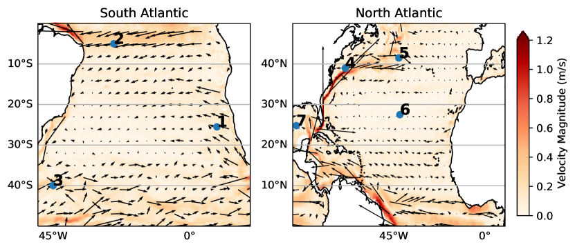
In Figure 1, we show seven locations plotted on a map with ocean currents. We use these locations as a proof-of-concept example throughout this paper. The exact coordinates are given in Table 1. The aim is to introduce and motivate a method which provides an estimate as to how long it would take to drift between any two of these locations. For example, the travel time from location 2 to location 3 in the South Atlantic Ocean should be smaller than the return journey due to the Brazil current. We choose to include locations in both the North and South Atlantic as we wish to demonstrate that the method successfully finds pathways linking points which are extremely far apart.

Figure 1: Locations of interest from Table 1. Annual mean values of the near-surface currents derived from drifter velocities (Laurindo et al., 2017) are plotted. Arrows drawn on a $3^{\circ}\times 3^{\circ}$ grid to show current direction.

1.1 Comparison with Related Works

In this section we give a brief overview of techniques that have used the Global Drifter Program to achieve a similar or related task. The work by Rypina et al. (2017) proposes a statistical approach for obtaining travel times. A source area is defined such that at least 100 drifters pass through the source area. The method focuses on obtaining a spatial probability map and a mean travel time for every $1^{\circ}\times 1^{\circ}$ bin outside of the source area. This method successfully combines many trajectories, however for multiple locations one would have to decide on a varying grid box for each location of interest. Such a grid box must be manually chosen by the practitioner meaning that the method does not scale well with multiple locations. Rypina et al. (2017) also focus on estimating a mean travel time, where our method provides a travel time associated with the most likely path, and is hence more akin to estimating a mode or median travel time.

The method by van Sebille et al. (2011), which proposes the use of Monte Carlo Super Trajectories (MCST), could naturally be used to estimate travel times. This method simulates new trajectories as sequences of unique grid indices along with corresponding travel time estimates for each part of that journey. The method is purely data driven i.e. they only use real trajectories to fit the model. The travel time and pathway we supply here should be similar to the most likely MCST to occur between the two points. The advantage of our methodology is that we do not base the analysis on a simulation, such that the results from the method described in Section 3 are not subject to any randomness due to simulation.

Various other works have made attempts to compute Lagrangian based distances. For example, Berline et al. (2014) used numerically simulated trajectories to estimate Mean Connection Times within the Mediterranean Sea. Smith et al. (2018) used MCST to estimate various statistics of how seagrass fragments could drift from the South East coast of Australia to Chile. Specifically, Smith et al. (2018) simulated 10 million MCST starting from the SE coast of Australia and only 264 (0.00264%) of the simulated trajectories were found to travel roughly to the Chilean coast.

The approach by Jönsson and Watson (2016) uses simulated drifter data to construct connectivity matrices between locations in the ocean. As the matrix is sparse, Dijkstra’s algorithm is used to connect arbitrarily distant locations in the ocean to measure Lagrangian distance. Although this method may at first glance bare similarities with our method (specifically in the use of Dijkstra’s algorithm), there are in fact many differences. First of all, the method uses simulated trajectories whereas we use real drifter trajectories. Secondly, Dijkstra’s algorithm is performed by Jönsson and Watson (2016) on the connectivity matrix (which finds minimum connection times between locations), whereas our approach uses Dijkstra’s algorithm on the transition matrix which describes a probabilistic framework for drifter movement. We found the latter approach to perform much better with real data. Finally, we cannot directly implement the approach described in Jönsson and Watson (2016) as only connectivity values higher than one year are used by the algorithm. For real data such a step would result in a very sparse connectivity matrix making the method infeasible. An initial analysis we conducted using similar methodology achieved poor results.

There are a variety of works which use Markov transition matrices for different aims to this work. Ser-Giacomi et al. (2015b) and Miron et al. (2019) look at probable paths, where both of these works find a path going between two points in a certain number of days using a dynamic program. Froyland et al. (2014) and Miron et al. (2017) study ocean dynamics by analysing eigenvalues of the transition matrix. Other methods in the literature include characterizing dispersion and mixing (Ser-Giacomi et al., 2015a), identification coherent regions (Froyland et al., 2007; Ser-Giacomi et al., 2015a), forward integration of tracers (van Sebille et al., 2012; Maximenko et al., 2012), and guiding drifter deployments (Lumpkin et al., 2016). We differ from these works as we ultimately aim to find travel times, as well as pathways, between multiple fixed locations.

Our proposed algorithm for computing travel times and pathways will also use the aforementioned Markov transition matrix approach. Our key novelty is that we build on this conceptual approach by implementing and demonstrating the benefits of using the (H3) spatial indexing system for discretization, and by supplying uncertainty quantification guidelines by applying grid rotations and data bootstrapping. The steps outlined in Algorithm 1 are individually known across disparate literature, however, this is the first paper to our knowledge that effectively combines these steps to solve the problem of interest. We provide numerous examples to show how our methodology robustly outperforms state-of-the-art alternative approaches. In addition, we supply freely-available software in the form of a Python package, of which all parameters in the model can easily be customized to suit the needs of the practitioner.

In summary, the novel contributions of this work are: a) the combination of the steps in Section 3 to form a computationally-efficient algorithm which applies directly to transition matrices to find most likely paths and travel times simultaneously, b) computation of uncertainty from discretization error and data sampling (Section 4), and c) the demonstration of the method showing it successfully obtains robust measures of connectivity between both very distant and closely located points (Section 5). The key outcome is that we obtain oceanographic travel times and most likely paths requiring no simulated trajectories.

We believe our method is preferable to Rypina et al. (2017) as we do not require custom treatment to different source areas. Jönsson and Watson (2016) requires the simulation of many very long and expensive to compute trajectories which obtain spurious results on real data. Using MCST’s as in Smith et al. (2018) relies on simulation. The estimation of a full pairwise travel time matrix of the locations in Table 1 requires 42 travel time estimations. With MCSTs this would likely require the simulation of millions of trajectories and manual analysis of each location pair. Our method, in contrast, can produce such a travel time matrix in a matter of seconds given that the transition matrix needs to be estimated just once a priori. In a similar manner, global travel time maps can be made in a matter of minutes, such as those that we will be showing in Section 5.

2 Background and Notation

2.1 Global Drifter Program

The Global Drifter Program(GDP) is a database managed by the National Oceanographic and Atmospheric Administraction (NOAA) (Lumpkin and Centurioni, 2019; Lumpkin and Pazos, 2007). This data set contains over 20,000 free-floating buoys temporally spanning from February 15, 1979 through to the current day. These buoys are referred to as drifters. The drifter design comprises of a sub-surface float and a drogue sock. Often this drogue sock detaches. We refer to the drifters which have lost their drogue sock as non-drogued drifters, and drogued for those which still have the drogue attached.

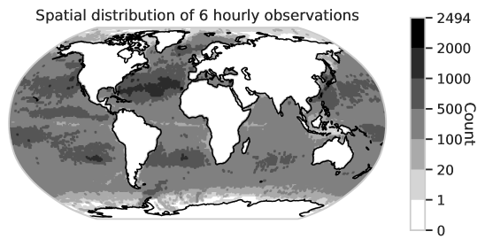
Here we use the drifter data recorded up to July, 2020. We use data which has been recorded from drogued drifters only. This results in a total of 23461 drifters being used, where the spatial distribution of observations is shown in Figure 2. Only using drogued drifters is not a restriction, it would be straightforward to simply use the data from non-drogued drifters if a practitioner was interested in a species or object which experiences a high wind forcing, or a combination of both if it is believed that the species followed a mixture of near surface and wind-forced currents. The data is quality controlled and interpolated to six hourly intervals using the methodology from Hansen and Poulain (1996). These interpolated values do contain some noise due to both satellite error and interpolation, however, the magnitude of this noise is negligible in comparison to the size of grid we use in Section 3. Hence, we ignore this noise and treat the interpolated values as observations. For the same reason we note that the interpolation method used is not important here, instead of the six hourly product we could use the hourly product produced by methodology proposed by Elipot et al. (2016), or drifter data smoothed by splines as proposed by Early and Sykulski (2020).

The value of using the Global Drifter Program is we obtain a true model-free representation of the ocean. All phenomena which act on the drifters are accounted for in the data set. The other common approach is to first obtain an estimate of the underlying velocity field, then simulate thousands of trajectories using the velocity field. While this simulation approach is often satisfactory in some applications, the models generally do not agree completely with the actual observations.

Figure 2: Number of observations from the Global Drifter Program in each $1^{\circ}\times 1^{\circ}$ longitude-latitude box.

2.2 Notation

Here we use $x^{\circ},y^{\circ}$ to be a geographic coordinate corresponding to latitude and longitude respectively. We refer to the longitude-latitude grid system using the notation $x^{\circ}\times y^{\circ}$, which means each grid box goes $x^{\circ}$ along the longitude axis and $y^{\circ}$ along the latitude axis. We use bold font for any data which is in longitude-latitude pairs; i.e $\textbf{r}=r_{lon},r_{lat}$, and non-bold text for either a grid index or a single number. We use $\mathcal{S}$ to denote the set of all possible grid indices. A full table of notation is given in Appendix B.

2.3 Capturing Drifter Motion

We define the drifter’s probability density function as

$$P(\mathbf{r}_{1},t\>|\>\mathbf{r_{0}},t_{0})$$

where the drifter started at $\mathbf{r_{0}}\in\mathbb{R}^{2}$ at time $t_{0}$ and moved to position $\mathbf{r}_{1}\in\mathbb{R}^{2}$ at time $t$, where $\mathbf{r}_{0}$ and $\mathbf{r}_{1}$ are longitude-latitude pairs. In the absence of a model, this probability density cannot be estimated continuously from data alone. Therefore, we follow previous works which spatially discretize the problem (Maximenko et al., 2012; van Sebille et al., 2011; Miron et al., 2019; Rypina et al., 2017; Lumpkin et al., 2016). Instead of considering $\mathbf{r}_{0}\in R^{2}$, we consider $r_{0}\in\mathcal{S}$ where $\mathcal{S}$ is some set of states which correspond to a polygon in space; we will define how these are formed in Section 3.2. Often these states are simply $1^{\circ}\times 1^{\circ}$ degree boxes (e.g. as used in Figure 2). As in Maximenko et al. (2012), we assume that the process driving the drifter’s movement is temporally stationary. That is:

$$P(r_{1},t\>|\>r_{0},t_{0})=P(r_{1}\>|\>r_{0},t-t_{0}),\quad r_{0},r_{1}\in\mathcal{S},$$

i.e. the probability of going from ${r}_{0}$ to ${r}_{1}$ depends only on the time increment. The probability does not depend on the start or finish time.

Furthermore, given that we are using data which is observed at regular and discrete times, we shall only consider discrete values of time. Let $\mathbf{s}=\{s_{0},s_{1},s_{2},\dots,s_{n}\}$ be a sequence of locations equally spaced in time where each entry $s_{i}$ can take the value of anything within $\mathcal{S}$. We define the probability $p(s_{i+1}=q\>|\>s_{i}=k)$ as the probability that the position at time $i+1$ is $q$ given that the state at time $i$ was $k$ where $q,k\in\mathcal{S}$.

A Lagrangian decorrelation time causes the drifter to ‘forget’ its history (LaCasce, 2008). We aim to choose a quantity which is globally higher than the Lagrangian decorrelation time. The reasoning behind using this time is that if we consider a sequence of observations, which are at least the Lagrangian decorrelation time apart then the following Markov property is satisfied:

$$p(s_{i+1}=q_{i+1}|s_{i}=q_{i},s_{i-1}=q_{i-1},\dotsm,s_{0}=q_{0})$$

$$= p(s_{i+1}=q_{i+1}\>|\>s_{i}=q_{i}),$$ (1)

where $q_{i}$ is just some fixed state and $s_{i}$ is the random process. In other words, the Markov property states that probability of transition to state $s_{i+1}$ is independent of all the past states at times $i-1$ and earlier, given the state at time $i$ is known. In this case, the physical time difference associated with $i+1$ and $i$ being larger than the chosen Lagrangian decorrelation time validates the use of the Markov assumption.

For the rest of this paper we assume that the time between discrete time observations is equal to $\mathcal{T}_{L}$. We call this quantity the Lagrangian cut off time. Setting $\mathcal{T}_{L}$ higher than the decorrelation time allows us to use the Markov property from Equation 1 freely. In so doing, alongside the simplification of discretizing locations, this allows the problem to be treated as a discrete time Markov chain. Here we fix $\mathcal{T}_{L}=5$ days as this matches previous similar works (Maximenko et al., 2012; Miron et al., 2019). The estimated decorrelation time for the majority of the surface of the Ocean is likely to be lower than 5 days (e.g. see Zhurbas and Oh (2004) for the Pacific and Lumpkin et al. (2002) for regions in the Atlantic). In Appendix E we conduct a sensitivity analysis to show our results are not overly sensitive to the choice of $\mathcal{T}_{L}$ as long as $\mathcal{T}_{L}>2$ days.

3 Method for Computing the Most Likely Path and Travel Time

Maximenko et al. (2012) and van Sebille et al. (2012) focus on the use of a transition matrix estimated from drifters to discover points where drifters are likely to end up. In this section we build on such an approach by providing a method to take such a matrix and provide an ocean pathway and travel time.

In Section 3.1, we explain in detail how the transition matrix is formed. As a grid system is needed to form the discretization of data we introduce our chosen system in Section 3.2. Then in Section 3.3, we describe how we estimate the most likely path of a drifter to have taken. Finally, in Section 3.4 we explain how we turn the most likely path and transition matrix into an estimate of travel time. We give a summary of how this articulates in the pseudo-code in Algorithm 1.

3.1 Transition Matrix

The location of a drifter at any given time is a continuous vector in $\mathbb{R}^{2}$, the longitude and latitude of the point. We define an injective map which maps this continuous process onto a discrete set of states which are indexed by integers in $\mathcal{S}$. We define the map as follows:

$$f:\mathbb{R}^{2}\rightarrow\mathcal{S}.$$ (2)

We aim to make a Markov transition matrix $T$ of size $n_{states}$ rows and columns, where $T_{s,q}$ denotes, the probability of moving from $s$ to $q$ in one time step. Similarly to the approach of Maximenko et al. (2012), we form our transition matrix using a gap method. In each drifter trajectory we only consider observations as a pair of points $\mathcal{T}_{L}$ days apart. When using this method for other applications we advise using $\mathcal{T}_{L}$ to be higher than the decorrelation time of velocity to justify the Markov assumption.

Consider a trajectory as a sequence of positions $\mathbf{y}_{j}=\{\mathbf{y}_{i,j}\}_{i=1}^{n_{j}}$ where $j$ is the $j^{th}$ out of $N$ trajectories, $n_{j}$ is the number of location observations in the trajectory, and $\mathbf{y}_{i,j}\in\mathbb{R}^{2}$ are the longitude-latitude positions. First, we map each trajectory into observed discrete states. We will denote these states as follows,

$$g_{i,j}=f(\mathbf{y}_{i,j}).$$ (3)

For each $s,p\in\mathcal{S}$ we estimate the relevant entry of our transition matrix $T$ through using the following empirical estimate:

$$T_{s,p}=\dfrac{\sum_{j=1}^{N}\sum_{i=1}^{n_{j}-4\mathcal{T}_{L}}\mathbb{I}[g_{i+4\mathcal{T}_{L},j}=p]\mathbb{I}(g_{i,j}=s)}{\sum_{j=1}^{N}\sum_{i=1}^{n_{j}-4\mathcal{T}_{L}}\mathbb{I}[g_{i,j}=s]},$$ (4)

Where $\mathbb{I}$ is the indicator function, such that it takes the value 1 if the statement inside it is true, and zero otherwise. Note that we take gaps of $4\mathcal{T}_{L}$ as observations are every 6 hours in the GDP application and $\mathcal{T}_{L}$ is in days. The estimation of the transition matrix, using the discretization of trajectories in Equation 3, in combination with Equation 4, is commonly referred to as Ulam’s approach (Ulam, 1960). We expect that states in $\mathcal{S}$ which are not spatially close will have non-zero entries such that the matrix $T$ will be very sparse, but this is not a problem for the methodology to work over large distances as we shall see.

3.2 Spatial Indexing

Clearly the resulting transition matrix described in Section 3.1 strongly depends on the choice of grid function in Equation 2. Most previous works (van Sebille et al., 2012; Maximenko et al., 2012; Rypina et al., 2017; McAdam and van Sebille, 2018; Miron et al., 2019) use longitude-latitude based square grids where all grid boxes typically vary between $0.5^{\circ}\times 0.5^{\circ}$ and $1^{\circ}\times 1^{\circ}$. A $1^{\circ}\times 1^{\circ}$ grid cell around the equatorial region will be approximately equal area to a $111.2\text{km}\times 111.2\text{km}$ square box. However, if we take such a grid above $60^{\circ}$ latitude, e.g. the Norwegian sea, the grid cell will be approximately equal area to a $55.6\text{km}\times 111.2\text{km}$ square box.

There are a few other choices which we argue are more suitable for tracking moving data on the surface of the Earth. Typically three types of grids exist for tessellating the globe: triangles, squares, or a mixture of hexagons and pentagons. Here we choose to use hexagons and pentagons as they have the desirable property that every neighbouring shape shares precisely two vertices and an edge. This is different to say a square grid where only side-by-side neighbours share two vertices and an edge, whereas diagonal neighbours share only a vertex. This equivalence of neighbors property for hexagons and pentagons is clearly desirable for the tracking of objects as this will result in a smoother transition matrix.

Figure 3: A small area around the Strait of Gibraltar which is tessellated using the H3 spatial index. We show resolutions 1, 2 and 3 in red, blue and black respectively. Black is the resolution used in this work.

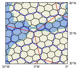
We specifically use the grid system called H3 by UBER (UBER, 2019). This system divides the globe such that any longitude and latitude coordinate is mapped to a unique hexagon or pentagon. This shape will have a unique geohash which we can use to keep track of grid index. The benefit of using such a spatial indexing system is that attention is paid to ensuring that each hexagon is approximately equal area. We use the resolution 3 index where each hexagon has an average area of $12,392\text{km}^{2}$. A square box of size $111.32\text{km}\times 111.32\text{km}$ has roughly the same area as this which is very similar to the size of a $1^{\circ}\times 1^{\circ}$ grid cell near the equator. An example of an area tessellated by H3 is shown in Figure 3. Other potential systems which could be used include S2 by Google which is a square system, or simply using a longitude-latitude system as various other works do. We show some example pathways using different grid systems and resolutions in the Supplementary Information Figure S1. The longitude-latitude system results in pathways that unrealistically follow long block-wise vertical or horizontal straight line motions, in contrast to the more realistic and meandering pathways produced by the hexagonal-pentagonal H3 grid system.

3.3 Most Likely Path

For our analysis, the first step is to define a most likely path. A path is simply a sequence of states such that the first element is the origin and the last element is the destination. We also require that two neighboring states are not equal to each other.

Definition 1 (Path).

We define the space of possible paths $\mathcal{P}_{o,d}$, between the origin $o\in\mathcal{S}$ and destination $d\in\mathcal{S}$, as the following:

$$\mathcal{P}_{o,d} =\{\mathbf{p}=(p_{0},p_{1},p_{2},\dots,p_{n}):p_{i}\in\mathcal{S}$$

$$\forall i\in\{1,\dots,{n-1}\},\ p_{0}=o,\ p_{n}=d,p_{i-1}\neq p_{i}\}.$$

With a cardinality operator $|\mathbf{p}|=n$ which denotes the length of the path.

Given the transition matrix $T$ we define the probability of such a path:

$$P(\mathbf{p})=\prod_{i=0}^{n-1}P(s_{i+1}=p_{i+1}\>|\>s_{i}=p_{i})=\prod_{i=0}^{n-1}T_{p_{i},p_{i+1}}.$$ (5)

Definition 2 (Most likely path).

Consider any path $\mathbf{p}\in\mathcal{P}_{o,d}=\{p_{0},p_{1},p_{2},\dots,p_{n}\}$. By the most likely path $\hat{\mathbf{p}}$ we mean the path which maximises the probability of observing that path.

$$\hat{\mathbf{p}}=\operatorname*{arg\,max}_{\mathbf{p}\in\mathcal{P}_{o,d}}\left\{P(\mathbf{p})\right\}=\operatorname*{arg\,max}_{\mathbf{p}\in\mathcal{P}_{o,d}}\left\{\prod_{i=0}^{n-1}T_{p_{i},p_{i+1}}\right\}.$$ (6)

Optimising Equation 6 appears intractable at first glance. However, this can easily be solved with shortest path algorithms such as Dijkstra’s algorithm (Dijkstra, 1959). We give precise details on how to find this pathway in Appendix C.

3.4 Obtaining a travel time estimate

The most likely path is often a quantity of interest in itself, however we can also obtain a travel time estimate of this path. The method should be fast and efficient as it should be able to run for large sets of locations quickly. We achieve this by giving a formula to estimate the travel time based directly on the transition matrix.

Consider the path, $\mathbf{p}=\{p_{1},\dots,p_{n}\}$, from which we aim to estimate the expected travel time. The key consideration this section addresses is: the path is a sequence of unique states, whereas when simulating from a discrete time Markov chain, the chain has a probability of remaining within the same state for multiple time steps. We therefore aim to obtain an estimate of how long the Markov chain takes, on average, to jump between $p_{i}$ and $p_{i+1}$, and then aggregate this over the path to form a travel time estimate.

We assume that the only possibility is that the drifter follows the path we are interested in. So $p_{i}$ must be followed by $p_{i+1}$. Now we use $t$ to index the time of the Markov chain and suppose $s_{t}=p_{i}$. We are then interested in the random variable $k$ where $t+k$ is the first time that the process transitions from $p_{i}$ to $p_{i+1}$. Note that the only possibility for states $\{s_{t+l}\}_{l=1}^{k-1}$ is that they are all $p_{i}$, otherwise the object would not be following the path of interest. Therefore, we obtain the distribution of $k$ as follows (proof in Appendix D.1):

$$P(s_{t+k}=p_{i+1},\{s_{t+l}=p_{i}\}_{l=1}^{k-1}\>|\>s_{t}=p_{i},\mathbf{p}\})$$

$$=\dfrac{T_{p_{i},p_{i+1}}T_{p_{i},p_{i}}^{k-1}}{(T_{p_{i},p_{i}}+T_{p_{i},p_{i+1}})^{k}}.$$ (7)

Note that if we set $a=\dfrac{T_{p_{i},p_{i}}}{T_{p_{i},p_{i}}+T_{p_{i},p_{i+1}}}$ in Equation 7 we get:

$$P(s_{t+k}=p_{i+1}\>|\>s_{t}=p_{i},\mathbf{p})=a^{k-1}(1-a),$$ (8)

which is the probability distribution function of a negative binomial distribution with success probability $a$ and number of failures being one. We denote the random variable for the travel time between $p_{i}$ and $p_{i+1}$ as $k_{i}$. As the negative binomial distribution corresponds to the time until a failure, we are interested in taking one time increment longer than this as we require $k_{i}$ to be the time that we move from $p_{i}$ to $p_{i+1}$ i.e. the time of the failure. Therefore the distribution of $k_{i}$ exactly follows $k_{i}-1\sim\text{NB}(1,a)$. Also, note that $k_{i}$ is in units of the chosen Lagrangian cutoff time $\mathcal{T}_{L}$.

To get the expectation of the total Lagrangian travel time we consider the sum of all the individual parts of the travel times $\mathbf{k}=\sum_{i=0}^{n-1}k_{i}$, such that we obtain:

$$\operatorname{\mathbb{E}}[\mathbf{k}]=\sum_{i=0}^{n-1}\operatorname{\mathbb{E}}[k_{i}]=\sum_{i=0}^{n-1}\left(\dfrac{T_{p_{i},p_{i}}}{T_{p_{i},p_{i+1}}}+1\right),$$ (9)

where we have used that the expectation of the negative binomial is $\operatorname{\mathbb{E}}[x\sim\text{NB}(1,a)]=\frac{a}{1-a}$.

We could attempt to obtain a simple variance estimate for the estimate $\operatorname{\mathbb{E}}[\mathbf{k}]$ with classical statistics. However, we would only be able to account for variability within the estimates of the entries $T$, as we would have to assume $\mathbf{p}$ is known. In our case we are interested in the time of $\hat{\mathbf{p}}$, which is itself an estimate as it depends on $T$. Obtaining any analytical uncertainty in the estimation of the most likely path would be intractable due to the complexity of the shortest path algorithm. Therefore, we propose to address the issue of uncertainty in $\operatorname{\mathbb{E}}[\mathbf{k}]$ and $\mathbf{p}$ due to data randomness in Section 4.2 using the non-parametric bootstrap. To finish this section, we provide the pseudo-code for our approach in Algorithm 1.

Input: Drifter data set $\mathbf{y}$, a set of locations $\mathbf{x}$, Lagrangian cutoff time $\mathcal{T}_{L}$

Map all the drifter locations $\mathbf{y}$ to their grids $g_{j,i}=f(\mathbf{y}_{j,i})$ using the map from Equation 2.

Map all the locations of interest to their grids $g^{x_{i}}=f(x_{i})$.

Form transition matrix $T$ using Equation 4.

for each unique pair $o$ and $d$ in $\{g^{x_{i}}\}_{x_{i}\in\mathbf{x}}$ do

       Find and store the most likely path $\hat{\mathbf{p}}_{o,d}$ by optimizing Equation (6).

       Using this path, find and store the expected travel time $\operatorname{\mathbb{E}}[\hat{\mathbf{k}}_{o,d}]$ using Equation 9.

      

end for

Result: Travel times $\operatorname{\mathbb{E}}[\hat{\mathbf{k}}_{o,d}]$ for every pair of locations in $\mathbf{x}$ and a corresponding path $\hat{\mathbf{p}}_{o,d}$ given as a sequence of grid indices in $\mathcal{S}$.

Algorithm 1 Pseudo-code which summarises how Section 3 is used to turn drifter data and a spatial index function into most likely paths and travel time estimates.

4 Stability and Uncertainty

4.1 Random Rotation

A key consideration is that the final results of the algorithmic approach may strongly rely on the precise grid system $f$ chosen in Equation 2. To address the uncertainty due to the discretization we propose to randomly sample a new grid system then run the algorithm for the new grid system. In a simple 2d square grid one could simply sample a new grid system by sampling two numbers between 0 and the length of a side of the square, then shifting the square by these sampled amounts in the $x$ and $y$ direction. In global complicated grid systems such as the one we consider here proposing uniform random shifting is not trivial.

Rather than trying to reconfigure the grid system, instead we suggest a more universal alternative. We suggest randomly rotating the longitude-latitude locations of all the relevant data using random rotations. Such a strategy will work for any spatial grid system as it just involves a prepossessing step of transforming all longitude-latitude coordinates. Note that for each rotation we are required to re-assign the points to the grid and re-estimate the transition matrix. These are the two most computationally expensive procedures of the method. To generate the random rotations we use the method suggested by Shoemake (1992). In summary, it amounts to generating 4 random numbers on a unit 4 dimensional hypersphere as the quaternion representation of the 3 dimensional rotation, which can equivalently be represented as a rotation matrix $M$. Then we apply this rotation to the Cartesian representation of longitude and latitude.

To obtain travel times which remove bias effects from discretization, we sample $n_{rot}$ rotation matrices $M^{(i)}$. We then run Algorithm 1, however as a prepossessing step we rotate all locations of the drifter trajectories and locations of interest. For each rotation matrix this will result in a set of travel times $\hat{d}^{(i)}$. The sample mean of these rotations will be more stable than the vanilla method. The sample standard deviation will inform us about uncertainty in travel times due to discretization.

4.2 Bootstrap

If we required a rough estimate of uncertainty we could consider that $\hat{\mathbf{p}}$, the most likely path, is fixed and then estimate $\operatorname{\text{Var}}[\hat{\mathbf{k}}]$. However, this would be a poor estimate because such an estimate would assume that: (1) the transition matrix entries follow a certain distribution, and (2) the path $\hat{\mathbf{p}}$ is the true most likely path. In reality neither of these are true, they will both just be estimates. The transition matrix elements are estimated from limited data and the shortest path strongly depends on the estimated transition matrix, e.g. a small change in the transition matrix could result in a significantly different path. Therefore, we obtain estimates of uncertainty by bootstrapping (Efron, 1993).

Bootstrapping is a method to automate various inferential calculations by resampling. Here the main goal is to estimate uncertainty around $\hat{\theta}=\operatorname{\mathbb{E}}[\hat{\mathbf{k}}]$. The bootstrap involves first resampling from the original drifters to obtain a new data set. We call $\mathbf{y}^{*}=\{\mathbf{y}_{j}^{*}\}_{j=1,\dots N}$ a bootstrap sample, where $\mathbf{y}_{j}^{*}$ is a drifter trajectory which has been sampled with replacement from the original $N$ drifters. Then we use $\mathbf{y}^{*}$ as the input dataset to Algorithm 1.

We do this resampling $B$ times to obtain $B$ estimates of $\hat{\theta}=\operatorname{\mathbb{E}}[\mathbf{\hat{k}}]$, we denote these bootstrap estimates as $\{\hat{\theta}^{(b)}\}_{b=1}^{B}$. We then estimate our final bootstrapped mean and standard deviation estimates as the following:

$$sd_{boot}^{2} =\left[\dfrac{\sum_{b=1}^{B}\left(\hat{\theta}^{(b)}-\hat{\theta}^{(.)}\right)^{2}}{B-1}\right],$$

$$\text{where}\quad\hat{\theta}^{(.)} =\sum_{b=1}^{B}\hat{\theta}^{(b)}/B.$$ (10)

In addition to the uncertainty measure in travel time that both the bootstrap and rotation methodology provide, these methods also supply a collection of sample most likely paths. These paths can be used to investigate various phenomena, such as why the uncertainty is high. We can plot the paths for a fixed origin-destination pair and may see for example that many paths follow one current where another collection of paths follow a different current. We give numerous examples of this in Sections 5.2 and 5.3.

5 Application

	Longitude	Latitude
1	9.0	-25.5
2	-25.0	-5.0
3	-45.0	-40.0
4	-69.0	39.0
5	-42.5	41.5
6	-42.0	27.5
7	-93.2	24.8

Table 1: Table of station locations

We use the locations given in Table 1 for the demonstration of the method described in this paper. These locations were chosen for multiple reasons; (1) they were placed on or near ocean currents, such as the South Atlantic current, the Equatorial current and the Gulf Stream; the magnitudes of which can be seen in Figure 1, and (2) stations were placed in both the North and South Atlantic to show how the method can find pathways which are not trivially connected. First we go over an application of the vanilla method from Section 3, then we provide brief results using the adaptations using bootstrap and rotations from Section 4 in Section 5.2 and Section 5.3 respectively. We supply a link to a Python package and code used to create these results in the Appendix.

Figure 4: Example pathways found from the method. Sequences of blue hexagons are going from the lower number to the higher number. Sequences of red hexagons are going from the higher number to the lower number. Numbered locations are as in Table 1. The expected travel time of the most likely path is given in the title of each plot. Similar plots can be provided for every location pair using the online code, however these are not presented here owing to page length considerations.

Prior to our analysis we take a practical step to improve the reliability of the method. we find the states corresponding to $-79.7^{\circ},9.07^{\circ}$, $-80.73^{\circ},8.66^{\circ}$ (two points on the Panama land mass), $-5.6^{\circ},36^{\circ}$ and $-5.61^{\circ},35.88^{\circ}$ (two points on the Strait of Gibraltar), then remove the corresponding rows and columns from $T$. If this step is not taken the method often uses pathways crossing the Panama land mass, resulting in impossibly short connections to the Pacific Ocean. The reasoning for removing the points on the Strait of Gibraltar is data-driven, further details are in the supplementary information, particularly how one can adapt the method to specify travel times into and out of the Mediterranean sea.

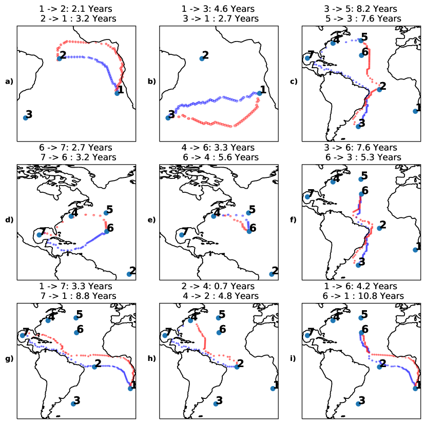
Figure 4 shows the pathways between a representative sample of the stations. First we note what features are observed in the most likely path. The Gulf Stream is used on almost every path trying to access locations 4, 5 or 6 in Figure 4. Observe in Figure 4 $c)$ when going from location 3 to 5 that the method chooses to enter the Gulf of Mexico and then uses the Gulf Stream to access location 5, even though the actual geodesic distance of this path is long. Other examples which use the Gulf Stream include $d)$ and $h)$. Generally, any of the paths leaving location 1 and attempting to travel northwest use the Benguela Current, for example Figure 4 $a)$, $i)$ and $g)$.

The travel times obtained between the sample stations in Figure 4 show interesting results regarding the lack of symmetry when reversing the direction of the path between two stations. When going from location 2 to location 4 we estimate a long most likely path in terms of physical distance. However, the resulting travel time of this path (0.7 years) is smaller than the travel time of the more direct path from location 4 to location 2 (4.8 years) - which is much shorter in distance. This is because the path going from location 2 to location 4 follows strong currents such as the North Equatorial current and the Gulf Stream. Another interesting result is that going from 3 to 5 and vice versa are relatively close in terms of travel time even though 3 to 5 uses the Gulf Stream but the return does not. In the most likely path from 3 to 5, up until around $-16^{\circ}$ latitude the travel time is 5.2 years, which we expect as the pathway seems to be going against the Brazil current. After this point the rest of the path takes the remaining 3 years despite the remainder being over half the actual physical distance of the pathway. We expect this short time is due to the method finding a pathway along the North Brazil current, followed by the Caribbean current, followed by the Gulf Stream.

Figure 5: Travel times of the most likely path originating from the red stars and going to or from (indicated by the title) the centroid of a $2.5^{\circ}\times 2.5^{\circ}$ square grid system. Figure setup and locations taken to match Figure 2 of Jönsson and Watson (2016).

5.1 Global Travel Times

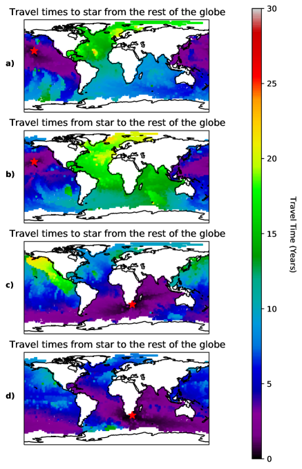
Figure 5 shows the travel time distribution to and from two fixed locations, taken to match the studied locations of Jönsson and Watson (2016), to the entire globe. We note that the travel time map is less smooth than the one shown in Jönsson and Watson (2016). The black and purple areas however (up to 5 years travel time) are similar to those found in Jönsson and Watson (2016), showing agreement over short spatial scales. When it comes to larger distances we generally find the maps are markedly different. For example the yellow patch in the north east pacific in Figure 5c is not seen in Jönsson and Watson (2016). Such discrepancies can be attributed to many reasons such as: (1) they reflect the difference in methods, where we use a transition matrix approach, and Jönsson and Watson (2016) use a connectivity matrix; (2) Jönsson and Watson (2016) aim to find the shortest path in time, whereas we aim to find the expected time of the most likely path; and (3) the results shown here are derived from real data, whereas Jönsson and Watson (2016) use simulated trajectories.

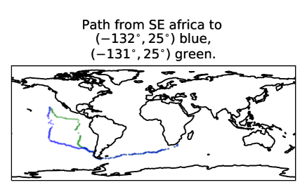
We show an example in Figure 6 which explains the lack of spatial smoothness in Figure 5, where we show two pathways both originating from a fixed point and ending at two distinct points only $1^{\circ}$ latitude apart. The points are on either side of the discontinuity in the north-east Pacific seen in Figure 5c. The pathways become visibly different after they have both reached the south Pacific. Such a phenomenon results in the lack of spatial smoothness of travel time distributions. This demonstrates that the travel times do not necessarily obey the triangle inequality. If smoothness is desired we show an alternative approach in the supplementary information, where instead a minimum travel time is the objective, which is then more analogous to the Jönsson and Watson (2016) approach. We argue however that the expected travel time of the most likely path, rather than the minimum travel time, is a more relevant metric for estimating connectivity and Lagrangian distance in applications measuring spatial dependence between points in the ocean.

Figure 6: The most likely path from two points in the North Pacific to the south-east coast of Africa. The green and blue pathways are almost identical as they cross the south Atlantic. The pathways differ greatly however as they cross the Pacific, even though the two starting points in the north Pacific are only 1 degree apart. The path going from $-131^{\circ},25^{\circ}$ has an expected travel time of 21.2 years, the path going from $-132^{\circ},25^{\circ}$ has an expected travel time of 11.4 years.

5.2 Bootstrap

To show the value of the bootstrap we show the results for one particular pair of stations, the pathway going from location 1 to location 3 and back. The pathways which result from the bootstrap are shown in the bottom panel of Figure 7. The darker lines on the figure imply that that this transition is used more often. We see that for most of the journey the darker lines closely follow the original path. The bootstrap discovers some slightly different paths, for example around $-20^{\circ}$ Longitude the path going from 3 to 1 occasionally seems to find that going further south is a more likely path. Also, around the beginning of the path going from 1 to 3, we see that the most likely path taken most frequently by the bootstrap samples often does not follow the most likely path from the full data.

Figure 7: Two bootstrap distributions of travel times are shown in the top row resulting from 200 bootstrap samples. The vertical line is the travel time if the full data is used to estimate the path and time. The corresponding bootstrapped paths are shown in the bottom figure. Blue lines and hexagons are for going from $1$ to $3$, red lines and hexagons are for going from $3$ to $1$. The lines connect the centroids of the spatial index of the bootstrapped paths. Darker lines mean that path is taken more often. The light hexagons are the pathway taken if the full data is used with no resampling i.e. the pathway shown in Figure 4.

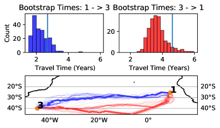
The main goal of the bootstrap is that we obtain an estimate of the standard errors. In this case we get standard error estimates using Equation 10 of 0.5 years for going from 3 to 1 and 0.6 years for going from 1 to 3. In general, we found that the standard error was lower when the path follows the direction of flow. The top row of plots in Figure 7 appears to show that there is a slight bias between the bootstrap mean and the vanilla method travel time. We believe this is due to the variance within the paths. The mean estimated from the bootstrap samples are close to the estimates from the rotation method we will shortly present in Figure 9. The rotation mean estimates are within 0.4 years of the bootstrap means in both cases shown here.

5.3 Rotation

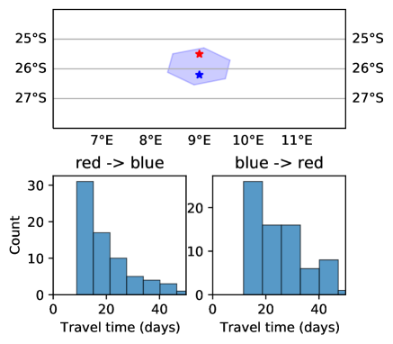
If we consider two points in the same H3 Index, for example location 1 ($9^{\circ},-25.5^{\circ}$) and a new point $9^{\circ},-26.2^{\circ}$ (as shown in Figure 8), then using the original grid system the method will simply produce a travel time of 0. To solve this problem, we consider using 100 rotations as explained in Section 4.1. For each rotation we estimate the travel time both back and forth. In 22 of the rotations the two points ended up in the same hexagon, hence resulting in a zero travel time. We plot the distribution of the other 78 travel times in the bottom row of Figure 8. The mean of all the entries including the zeros is 20.5 days for going from the new point to location 1, and 22.2 days for going from location 1 to the new point.

Figure 8: Plot of location 1 from Table 1 and the point $9^{\circ},-26.2^{\circ}$, which is $0.7^{\circ}$ south of location 1. The relevant H3 hexagon is plotted over the points. In the bottom row we plot the histogram and density estimate of the travel times in each direction from applying 100 rotations. The 22 zeros for when the two locations are in the same hexagon are not included in the histogram.

Figure 9: This figure layout is the same as in Figure 4, except here we plot paths resulting from 100 random rotations. Each line connects the centroid of each hexagon within the path. Note that the hexagons now come from rotated grid systems, so the centroids could be at any location hence the smooth continuous looking lines. The lines are plotted with transparency, when multiple lines overlap these lines will look darker. Standard deviations of the travel times of the 100 paths are reported in the title of each figure.

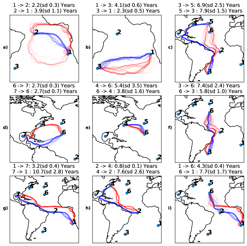
The second benefit of performing rotations is to make estimates less dependent on the grid system. We use the same 100 rotations as with the previous example, and compute the most likely path and the mean travel times. In Figure 9 we plot the pathways with the mean and standard deviation of the travel times resulting from these 100 rotations. The travel times and paths shown in this figure are comparable to those given in Figure 4. In most of the pathways we see that the darkest, most popular paths match up with the pathways in Figure 4.

One of the more interesting results from this analysis is the path going from $2$ to $1$ in Figure 9 a). Most of the paths go up closer to the Equator, then use the Equatorial Counter current, followed by the Guinea and Gulf of Guinea currents as in the original vanilla application of the methodology. A small number of the rotations result in pathways that end up crossing the South Atlantic, to the south of location 2, then follows the South Atlantic current over to location 1.

In general, the travel times from the rotation and original method can be significantly different, which supports the need for this rotation methodology. If we compare Figure 4 and Figure 9, most of the distances stay close to what they were in the original results using no rotations. We see that going from 6 to 4 drops from 5.6 years in Figure 4e) to 3.8 years in Figure 9e) and 4 to 6 increases from 3.3 years to 5.4 years. This causes the ordering of the distances to change as 6 to 4 is now the shorter travel time. We believe the case in e) is mainly due to 4 being located just north west of the stronger currents of the Gulf Stream, which makes it sensitive to the grid system. However, the high standard errors in Figure 9 suggest we are uncertain about this travel time.

6 Discussion and Conclusion

In contrast to van Sebille (2014), our methodology as presented does not take into account seasonality. We have a few ideas for how seasonality could be incorporated in future work. An obvious adaptation, if the aim was to obtain a short travel time which is expected to lie in a small 3 month window, is to just estimate $T$ using drifter observations which are in that time window. Alternatively, we could use $\mathcal{T}_{L}$ to be a certain jump such as a gap of two months, then we estimate 6 transition matrices say $T^{(k)}$, where the entries $T^{(k)}_{i,j}$ are probabilities of going from the previous time period at state $i$ to state $j$ at the current time. Such a set up could still be solved using our shortest path algorithm. We justify our approach in the same way as Maximenko et al. (2012): we aim to provide a global view and a simple general concept explaining the pattern of potential pathways and travel times. The base method can then be adapted by practitioners to account for local spatial or temporal considerations.

More results demonstrating the robustness of our method, and motivation of parameter choices, can be found in the supplementary information. A key finding we discuss here, is that we found the size of the grid system affects the estimated travel times significantly, regardless of whether the lat-lon or the H3 grid system is used. Therefore we do not recommend comparing travel times obtained from two different grid sizes. Generally the results are correlated in an order comparison sense, however, their magnitudes change. Typically a smaller grid system results in shorter travel times. Due to this we would only advise the results to be used in relative comparison to each other, for example by saying that the travel time from $a$ to $b$ is twice that than from $b$ to $c$, where both times are obtained with the same grid system. The choice to show resolution 3 in this paper was found to perform robustly (balancing the error from discretisation and data sparsity), and follows grid sizes that approximately match previous works where $1^{\circ}\times 1^{\circ}$ grids are used, but this can be changed easily in the online package.

The use of the bootstrap and rotations are relatively easy methods to implement, each of which provides effective estimates of uncertainty from data uncertainty and discretisation respectively. However, combining these procedures into one requires careful consideration. If we wanted to run $n_{rot}$ rotations and $B$ bootstraps for each rotation, we still require a method to combine these estimates of travel times. We could treat every rotation equivalently, so say that our bootstrap sample in Equation 10 is all $n_{rot}\times B$ samples to obtain an estimate of uncertainty in travel time due to the combination of grid discretization and data randomness. Additionally, we could decompose the uncertainty and provide a standard error for just the data randomness by estimating a standard error for each rotation using just the $B$ samples in each rotation, and then taking the average of all $n_{rot}$ standard error estimates.

Our choice of the Lagrangian decorrelation time of 5 days may be too low in some instances. Previous works have found correlations in the velocity data lasting longer than $5$ days in certain regions (Lumpkin et al., 2002; Zhurbas and Oh, 2004; Elipot et al., 2010). This may suggest that using a larger value for $\mathcal{T}_{L}$ may be needed to justify the Markov assumption. The tradeoff however is resolution, where shorter timescales allow pathways and distances to be computed with more detail. Our methodology is designed flexibly such that the practitioner can pick the most appropriate timescale for the spatial region and application of interest.

In general some unexpected features of the method do occur such as the discontinuity discussed in Section 5.1. We expect there would be less of a discontinuity if these times were computed with the rotation methodology, however we argue that the discontinuities with travel times of most likely pathways should always exist. If smoothness of travel times was a major requirement, then one could consider the shortest path in travel time rather than the most likely path. We briefly show this adaptation in the supplementary information. We expect the results would require more careful checking in such an approach, as the shortest path would be more likely to use any glitches in the grid system such as if there was a connection over Panama.

To summarize, in this paper we have created a novel method to estimate Lagrangian pathways and travel times between oceanic locations, thus offering a new, fast and intuitive tool to improve our knowledge of the dynamics of marine organisms and oceanic transport and global circulation.

Acknowledgments

The work of M. O’Malley was funded by the Engineering and Physical Sciences Research Council (Grant EP/L015692/1). The work of A. M. Sykulski was funded by the Engineering and Physical Sciences Research Council (Grant EP/R01860X/1).

Data Availability Statement

The drifter data were provided by the Global Drifter Program (Lumpkin and Centurioni, 2019). The currents used for visualisation purposes in Figure 1 are V3.05 of the dataset supplied on the Global Drifter Program website (Laurindo et al., 2017).

Appendix A Package

Code to reproduce all figures related to the method is available at https://github.com/MikeOMa/MLTravelTimesFigures which depends on the python package implementing all of the above methods in this paper at https://github.com/MikeOMa/DriftMLP. The package takes roughly 3 minutes total to go from raw data to a pairwise travel time matrix for the locations shown in Table 1 using Algorithm 1.

Appendix B Table of Notation

We include a table of mathematical notation for reader reference in Table 2.

$P(x\>|\>y)$	denotes the probabilities of event(s) $x$ given that $y$ occurs.
$\operatorname{\mathbb{E}}[x]$	The expectation of $x$.
$f(s)$	The discretization function i.e. H3.
$\mathbb{I}(x)$	Indicator function giving 1 if $x$ is true and 0 otherwise.
$\operatorname*{arg\,max}_{x\in S}$	An operator which gives the input value, which maximises the function $q$, restricted to the set $S$.
$T$, $T_{i,j}$	$T$ denotes transition matrix, with entries $T_{i,j}$. $i,~{}j\in\mathcal{S}$, denoting the probability of moving from state $i$ to $j$ in $\mathcal{T}_{L}$ days.
$x^{\circ}\times y^{\circ}$	refers to a longitude-latitude grid system, $x$ degrees in the longitudinal direction, $y$ degrees in the latitudinal direction.
$\mathcal{T}_{L}$	Lagrangian cut off time.
$\mathcal{S}$	The set of all possible spatial indices.
$\mathcal{P}_{o,d}$	The set of all possible paths going from $o$ to $d$.
$\mathbf{p}=\{p_{i}\}_{i=1}^{n}$	A pathway of length $n$. Indicates a sequence $p_{1},~{}p_{2},\dots,p_{n}$. All $p_{i}\in\mathcal{S}$.
$\mathbf{k}$	The expected travel time of a path $\mathbf{p}$.
$\hat{\mathbf{p}}$, $\hat{\mathbf{k}}$	Hat notation implies we are considering the most likely path and travel time of that path respectively.
$s_{t}$	used to index the state of the Markov chain after $t$ steps.

Table 2: Table of mathematical notation.

Appendix C Finding the shortest path

To solve the optimization of Equation 6, we can equivalently consider the $log$ of $P(\mathbf{p})$:

$$\log P(\mathbf{p}) =\sum_{i=0}^{n-1}\log T_{p_{i},p_{i+1}}.$$

Then we use the fact that:

$$\hat{\mathbf{p}} =\operatorname*{arg\,max}_{\mathbf{p}\in\mathcal{P}_{o,d}}\left\{\log P(\mathbf{p})\right\}=\operatorname*{arg\,min}_{\mathbf{p}\in\mathcal{P}_{o,d}}\left\{-\log P(\mathbf{p}\right\})$$

$$=\operatorname*{arg\,min}_{\mathbf{p}\in\mathcal{P}_{o,d}}\left\{-\sum_{i=0}^{n-1}\log T_{p_{i},p_{i+1}}\right\}.$$ (11)

Now in this form this can be solved using the vast literature on shortest path algorithms.

Appendix D Shortest Path Algorithms

Shortest path algorithms (Gallo and Pallottino, 1988; Dijkstra, 1959), such as Dijksta’s algorithm, are popular algorithms which find the so called shortest path within a graph. In our case the graph is formed such that the vertices or nodes uniquely correspond to a grid system index, i.e. a row/column in the transition matrix $T$. If there is a non-zero probability in $T_{i,j}$ we add an edge denoted $e_{i,j}$, where the weight on this edge is denoted $w(e_{i,j})=-\log(T_{i,j})$ between the vertex $i$ and going to the vertex $j$. Note that $T_{i,j}$ is not necessarily the same as $T_{j,i}$, hence we have a directed graph. Given a start vertex $o$ and an end vertex $d$, shortest path algorithms will find the path $P=\{v_{1}\dots,v_{n}\}$ such that $P$ minimises the following

$$\sum_{i=1}^{n-1}w(e_{v_{i},v_{i+1}}),$$

hence it solves the problem in Equation 11. The algorithm used is exact, hence if no path is found then no path exists given the current network.

D.1 Derivation of Equation 7

The derivation uses the Markov property, the conditional probability definition, and the fact that $P(x\in\{a,b\})=P(x=a)+P(x=b)$.

$$P(s_{t+k}=p_{i+1},\{s_{t+l}=p_{i}\}_{l=1}^{k-1}\>|\>s_{t}=p_{i},\mathbf{p}\})$$

$$=P(s_{t+k}=p_{i+1}\>|\>s_{t+k-1}=p_{i},s_{t+k}\in\{p_{i},p_{i+1}\})$$

$$\quad\times\prod_{l=1}^{k-1}P(s_{t+l}=p_{i}\>|\>s_{t+l-1}=p_{i},s_{t+l}\in\{p_{i},p_{i+1}\})$$

$$=\dfrac{P(s_{t+k}=p_{i+1}\>|\>s_{t+k-1}=p_{i})}{P(s_{t+k}\in\{p_{i},p_{i+1}\}\>|\>s_{t+k-1}=p_{i})}$$

$$\quad\times\prod_{l=1}^{k-1}\dfrac{P(s_{t+l}=p_{i}\>|\>s_{t+l-1}=p_{i})}{P(s_{t+l}\in\{p_{i},p_{i+1}\}\>|\>s_{t+l-1}=p_{i})}$$

$$=\dfrac{P(s_{t+k}=p_{i+1}\>|\>s_{t+k-1}=p_{i})}{P(s_{t+1}\in\{p_{i},p_{i+1}\}\>|\>s_{t}=p_{i})^{k}}$$

$$\quad\times\prod_{l=1}^{k-1}P(s_{t+l}=p_{i}\>|\>s_{t+l-1}=p_{i})$$

$$=\dfrac{T_{p_{i},p_{i+1}}T_{p_{i},p_{i}}^{k-1}}{(T_{p_{i},p_{i}}+T_{p_{i},p_{i+1}})^{k}}$$

where the first equality follows from the explanation given in Section 3.4.

Appendix E Brief Sensitivity Analysis to cut off time

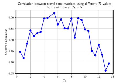
The main tuning parameter which we have fixed in this paper is the Lagrangian cut off time used when estimating the transition matrix $T$. The method is not especially sensitive to this choice as we shall now demonstrate. To show the sensitivity we ran an experiment where for a grid of values for $\mathcal{T}_{L}$ we estimated a pairwise travel time matrix for the locations in Table 1, then we estimated the Spearman correlation coefficient between the non-diagonal entries of each matrix to the corresponding entry of the travel time matrix generated from $\mathcal{T}_{L}=5$. Results are shown in Figure 10. The experiment shows that the distances change but overall the matrices are very strongly correlated, particularly for $\mathcal{T}_{L}>2$. For comparison the average correlation value between the the pairwise travel time matrix $\mathcal{T}_{L}$ and the travel time matrices generated from the 100 rotations used in Section 5.3 is 0.8. A similar analysis, considering sensitivity to grid sizes is given in the online supplementary information.

Figure 10: Spearman Correlation coefficient between the non-diagonal elements of the travel time matrix generated by $\mathcal{T}_{L}=5$ and the matrices generated by the values of $\mathcal{T}_{L}$ on the $x$-axis.

References

- Becking et al. (2006) Becking, L. E., D. F. Cleary, N. J. de Voogd, W. Renema, M. de Beer, R. W. van Soest, and B. W. Hoeksema, 2006: Beta diversity of tropical marine benthic assemblages in the Spermonde Archipelago, Indonesia. Marine Ecology, 27 (1), 76–88.
- Berline et al. (2014) Berline, L. O., A. M. Rammou, A. Doglioli, A. Molcard, and A. Petrenko, 2014: A Connectivity-Based Eco-Regionalization Method of the Mediterranean Sea. PLoS ONE, 9 (11), 1–9, doi:https://doi.org/10.1371/journal.pone.0111978.
- Dijkstra (1959) Dijkstra, E. W., 1959: A note on two problems in connexion with graphs. Numerische Mathematik, 1 (1), 269–271, doi:https://doi.org/10.1007/BF01386390.
- Early and Sykulski (2020) Early, J. J., and A. M. Sykulski, 2020: Smoothing and interpolating noisy GPS data with smoothing splines. Journal of Atmospheric and Oceanic Technology, 37 (3), 449–465.
- Efron (1993) Efron, B., 1993: An introduction to the bootstrap. Monographs on statistics and applied probability ; 57, Chapman & Hall, New York.
- Elipot et al. (2016) Elipot, S., R. Lumpkin, R. C. Perez, J. M. Lilly, J. J. Early, and A. M. Sykulski, 2016: A global surface drifter data set at hourly resolution. Journal of Geophysical Research: Oceans, 121 (5), 2937–2966, doi:http://doi.org/10.1002/2016JC011716.
- Elipot et al. (2010) Elipot, S., R. Lumpkin, and G. Prieto, 2010: Modification of inertial oscillations by the mesoscale eddy field. Journal of Geophysical Research: Oceans, 115 (9), 1–20, doi:https://doi.org/10.1029/2009JC005679.
- Ellingsen and Gray (2002) Ellingsen, K., and J. Gray, 2002: Spatial patterns of benthic diversity: Is there a latitudinal gradient along the Norwegian continental shelf? Journal of Animal Ecology, 71, 373 – 389, doi:https://doi.org/10.1046/j.1365-2656.2002.00606.x.
- Froyland et al. (2007) Froyland, G., K. Padberg, M. H. England, and A. M. Treguier, 2007: Detection of coherent oceanic structures via transfer operators. Physical review letters, 98 (22), 224 503.
- Froyland et al. (2014) Froyland, G., R. M. Stuart, and E. van Sebille, 2014: How well-connected is the surface of the global ocean? Chaos: An Interdisciplinary Journal of Nonlinear Science, 24 (3), 033 126.
- Gallo and Pallottino (1988) Gallo, G., and S. Pallottino, 1988: Shortest path algorithms. Annals of Operations Research, 13 (1), 1–79, doi:https://doi.org/10.1007/BF02288320.
- Hansen and Poulain (1996) Hansen, D. V., and P.-M. Poulain, 1996: Quality control and interpolations of WOCE-TOGA drifter data. Journal of Atmospheric and Oceanic Technology, 13 (4), 900–909.
- Huntley et al. (2011) Huntley, H. S., B. Lipphardt Jr, and A. Kirwan Jr, 2011: Lagrangian predictability assessed in the East China Sea. Ocean Modelling, 36 (1-2), 163–178.
- Jönsson and Watson (2016) Jönsson, B. F., and J. R. Watson, 2016: The timescales of global surface-ocean connectivity. Nature communications, 7 (1), 1–6.
- LaCasce (2008) LaCasce, J. H., 2008: Statistics from Lagrangian observations. Progress in Oceanography, 77 (1), 1–29.
- Laurindo et al. (2017) Laurindo, L. C., A. J. Mariano, and R. Lumpkin, 2017: An improved near-surface velocity climatology for the global ocean from drifter observations. Deep Sea Research Part I: Oceanographic Research Papers, 124, 73–92.
- Lumpkin and Centurioni (2019) Lumpkin, R., and L. Centurioni, 2019: Global Drifter Program quality-controlled 6-hour interpolated data from ocean surface drifting buoys. NOAA National Centers for Environmental Information. Accessed [2020-01-20], doi:https://doi.org/10.25921/7ntx-z961.
- Lumpkin et al. (2016) Lumpkin, R., L. Centurioni, and R. C. Perez, 2016: Fulfilling observing system implementation requirements with the global drifter array. Journal of Atmospheric and Oceanic Technology, 33 (4), 685–695.
- Lumpkin and Pazos (2007) Lumpkin, R., and M. Pazos, 2007: Measuring surface currents with surface velocity program drifters: The instrument, its data, and some recent results. Lagrangian analysis and prediction of coastal and ocean dynamics, 2, 39–67.
- Lumpkin et al. (2002) Lumpkin, R., A.-M. Treguier, and K. Speer, 2002: Lagrangian eddy scales in the Northern Atlantic Ocean. Journal of Physical Oceanography, 32 (9), 2425–2440, doi:https://doi.org/10.1175/1520-0485-32.9.2425.
- Maximenko et al. (2012) Maximenko, N., J. Hafner, and P. Niiler, 2012: Pathways of marine debris derived from trajectories of Lagrangian drifters. Marine Pollution Bulletin, 65 (1-3), 51–62, doi:https://doi.org/10.1016/j.marpolbul.2011.04.016.
- McAdam and van Sebille (2018) McAdam, R., and E. van Sebille, 2018: Surface connectivity and interocean exchanges from drifter-based transition matrices. Journal of Geophysical Research: Oceans, 123 (1), 514–532, doi:https://doi.org/10.1002/2017JC013363.
- Meehl (1982) Meehl, G. A., 1982: Characteristics of surface current flow inferred from a global ocean current data set. Journal of Physical Oceanography, 12 (6), 538–555.
- Miron et al. (2019) Miron, P., F. J. Beron-Vera, M. J. Olascoaga, and P. Koltai, 2019: Markov-chain-inspired search for MH370. Chaos: An Interdisciplinary Journal of Nonlinear Science, 29 (4), doi:https://doi.org/10.1063/1.5092132.
- Miron et al. (2017) Miron, P., F. J. Beron-Vera, M. J. Olascoaga, J. Sheinbaum, P. Pérez-Brunius, and G. Froyland, 2017: Lagrangian dynamical geography of the gulf of mexico. Scientific reports, 7 (1), 1–12.
- Rypina et al. (2017) Rypina, I. I., D. Fertitta, A. Macdonald, S. Yoshida, and S. Jayne, 2017: Multi-iteration approach to studying tracer spreading using drifter data. Journal of Physical Oceanography, 47 (2), 339–351, doi:https://doi.org/10.1175/JPO-D-16-0165.1.
- Ser-Giacomi et al. (2015a) Ser-Giacomi, E., V. Rossi, C. López, and E. Hernández-García, 2015a: Flow networks: A characterization of geophysical fluid transport. Chaos: An Interdisciplinary Journal of Nonlinear Science, 25 (3), 036 404.
- Ser-Giacomi et al. (2015b) Ser-Giacomi, E., R. Vasile, E. Hernández-García, and C. López, 2015b: Most probable paths in temporal weighted networks: An application to ocean transport. Physical review E, 92 (1), 012 818.
- Shoemake (1992) Shoemake, K., 1992: Uniform random rotations. Graphics Gems III (IBM Version), Elsevier, 124–132.
- Smith et al. (2018) Smith, T. M., and Coauthors, 2018: Rare long-distance dispersal of a marine angiosperm across the Pacific Ocean. Global Ecology and Biogeography, 27 (4), 487–496, doi:https://doi.org/10.1111/geb.12713.
- Sykulski et al. (2016) Sykulski, A. M., S. C. Olhede, J. M. Lilly, and E. Danioux, 2016: Lagrangian time series models for ocean surface drifter trajectories. Journal of the Royal Statistical Society. Series C: Applied Statistics, 65 (1), 29–50, doi:https://doi.org/10.1111/rssc.12112.
- UBER (2019) UBER, 2019: H3 spatial index. Accessed: 2020-01-08, https://eng.uber.com/h3/.
- Ulam (1960) Ulam, S. M., 1960: A collection of mathematical problems. Interscience tracts in pure and applied mathematics ; no. 8, Interscience Publishers, New York.
- van Sebille (2014) van Sebille, E., 2014: Adrift.org.au - A free, quick and easy tool to quantitatively study planktonic surface drift in the global ocean. Journal of Experimental Marine Biology and Ecology, 461, 317–322, doi:https://doi.org/10.1016/j.jembe.2014.09.002.
- van Sebille et al. (2011) van Sebille, E., L. M. Beal, and W. E. Johns, 2011: Advective time scales of Agulhas leakage to the North Atlantic in surface drifter observations and the 3D OFES model. Journal of Physical Oceanography, 41 (5), 1026–1034, doi:https://doi.org/10.1175/2011JPO4602.1.
- van Sebille et al. (2012) van Sebille, E., M. H. England, and G. Froyland, 2012: Origin, dynamics and evolution of ocean garbage patches from observed surface drifters. Environmental Research Letters, 7 (4), doi:10.1088/1748-9326/7/4/044040.
- van Sebille et al. (2009) van Sebille, E., P. van Leeuwen, A. Biastoch, C. Barron, and W. de Ruijter, 2009: Lagrangian validation of numerical drifter trajectories using drifting buoys: Application to the Agulhas system. Ocean Modelling, 29 (4), 269–276, doi:10.1016/J.OCEMOD.2009.05.005.
- van Sebille et al. (2018) van Sebille, E., and Coauthors, 2018: Lagrangian ocean analysis: Fundamentals and practices. Ocean Modelling, 121, 49–75, doi:https://doi.org/10.1016/j.ocemod.2017.11.008.
- Wakata and Sugimori (1990) Wakata, Y., and Y. Sugimori, 1990: Lagrangian motions and global density distributions of floating matter in the ocean simulated using shipdrift data. Journal of Physical oceanography, 20, 125–138.
- Watson (2018) Watson, J. R., 2018: The geography of the world’s oceans explains patterns of planktonic diversity. 2018 Ocean Sciences Meeting, AGU.
- White et al. (2010) White, C., K. A. Selkoe, J. Watson, D. A. Siegel, D. C. Zacherl, and R. J. Toonen, 2010: Ocean currents help explain population genetic structure. Proceedings of the Royal Society B: Biological Sciences, 277 (1688), 1685–1694.
- Zhurbas and Oh (2004) Zhurbas, V., and I. S. Oh, 2004: Drifter-derived maps of lateral diffusivity in the Pacific and Atlantic oceans in relation to surface circulation patterns. Journal of Geophysical Research: Oceans, 109 (C5).