Hierarchical Correlation Clustering and Tree Preserving Embedding
Abstract
We propose a hierarchical correlation clustering method that extends the well-known correlation clustering to produce hierarchical clusters applicable to both positive and negative pairwise dissimilarities. Then, in the following, we study unsupervised representation learning with such hierarchical correlation clustering. For this purpose, we first investigate embedding the respective hierarchy to be used for tree preserving embedding and feature extraction. Thereafter, we study the extension of minimax distance measures to correlation clustering, as another representation learning paradigm. Finally, we demonstrate the performance of our methods on several datasets.
1 Introduction
Data clustering plays an essential role in unsupervised learning and exploratory data analysis. It is used in a variety of applications including web mining, network analysis, user understanding, image segmentation, knowledge management, and bioinformatics. Its goal is to partition the data into groups in a way that the objects in the same cluster are more similar according to some criterion, compared to the objects in different clusters.
Some clustering methods partition the data into flat clusters for example via minimizing a cost function, e.g., -means [51], spectral clustering [64, 58] and correlation clustering [9]. In many applications, however, the clusters are desired to be presented at different levels, such that both high-level and detailed information are preserved. Therefore, hierarchical clustering is useful to produce such structures, usually encoded by a dendrogram. A dendrogram is a tree data structure wherein every node represents a cluster and the leaf nodes (i.e., the nodes linked to just one other node) include only one object. A cluster at a higher level consists of the union of the lower-level clusters, and the inter-cluster dissimilarity between them.
Hierarchical clustering can be performed either in an agglomerative (i.e., bottom-up) or in a divisive (i.e., top-down) manner [52]. Agglomerative methods are often computationally more efficient, making them more popular in practice [60]. In both approaches, the clusters are combined or divided according to different criteria, e.g., single, complete, average, centroid and Ward. Several methods aim to improve these methods. The work in [3] studies the locality and outer consistency of agglomerative algorithms in an axiomatic way. The works in [45, 48] focus on the statistical significance of hierarchical clustering. [21, 22, 61] investigate optimization methods for hierarchical clustering and propose approximate solutions. K-Linkage in [76] takes into account multiple dissimilarities for a pair of clusters. [7] employs global information to determine the inter-cluster similarities in order to eliminate the influence of noisy similarities, and [16] suggests using agglomerative methods on small dense subsets of the data, instead of the original data objects. The methods in [29, 34] investigate combining agglomerative methods with probabilistic models which then yields an extra computational complexity. Finally, [56, 20] develop efficient but approximate implementations of agglomerative methods.
On the other hand, most clustering methods, either flat or hierarchical, assume non-negative pairwise (dis)similarities. However, in several practical applications, pairwise relations are provided in the form of both positive and negative similarities. For example, it might be more convenient for a user/oracle to specify if two objects are similar (i.e., a positive relation) or dissimilar (i.e., a negative relation) instead of giving only a positive (non-negative) pairwise similarity even if the two objects are dissimilar. In addition, the former provides more accurate information, as in the latter case, the dissimilarity between two objects (i.e., zero similarity) might be confused with the lack of information. Assuming the pairwise similarities are provided by an oracle, then uncertainty can be handled better by this kind of data, where the oracle can explicitly distinguish between noise, uncertainty, and lack of similarity. Some relevant applications for this setting include image segmentation with higher order correlation information [43, 44], community detection over graphs [63], web people search via analysis of connections [39], working with attraction/rejection data [23], automated label generation from clicks [4], webpage segmentation [12], social media mining [69], and entity resolution [8, 30].
Thereby, a specific form of clustering model, called correlation clustering, has been developed to deal with such data. This model was first introduced on the graphs with only or pairwise similarities [9, 8], and then was generalized to the graphs with arbitrary positive or negative edge weights [23, 6, 13]. The original model obtains the number of clusters automatically. The variant in [17] limits the number of clusters to fixed clusters. Semidefinite programming (SDP) relaxation provides tight approximation bounds in particular for maximizing the agreements [13, 54], although it is computationally inefficient in practice [70]. Then, the methods in [15, 70] provide efficient greedy algorithms based on local search and Frank-Wolfe optimization with a fast convergence rate.
However, all of these methods produce flat correlation clusters. In this paper, we first propose a Hierarchical Correlation Clustering (HCC) method that handles both positive and negative pairwise (dis)similarities and produces clusters at different levels (Section 3). To the best of our knowledge, this work is the first generalization of the well-studied correlation clustering to hierarchical clustering.111We note the so-called hierarchical correlation clustering methods proposed in [2, 32, 49] are irrelevant to the well-studied correlation clustering problem [9, 8]; they study for example the correlation coefficients for high-dimensional data.
We note that unlike flat clustering, hierarchical clustering yields an ordering among the objects, i.e., objects that join earlier in the hierarchy are closer to each other than those that join at later steps. This implies that hierarchical clustering induces a new (dis)similarity measure between the objects, connected to the way the objects join each other to form clusters at different levels. Thereby, in the following, we consider two representation learning methods related to hierarchical clustering and study their adaptation to hierarchical correlation clustering. This enables us to not only use HCC for producing hierarchical clusters, but also to employ it for computing a suitable similarity/distance measure as an intermediate data processing step.
One way to perform representation learning from hierarchical clustering is to compute an embedding that corresponds to the respective hierarchy. Tree preserving embedding [65, 66] is a method that achieves this for the special case of single linkage method. Later, [18] develops tree preserving embedding for various standard agglomerative clustering methods. We then adapt these works to develop a tree preserving embedding for HCC dendrograms (Section 4) where the embedded features can be used as a set of new features for an arbitrary downstream task. In this way, we can investigate HCC for the purpose of computing relevant features for a probabilistic method such as Gaussian Mixture Model (GMM), instead of solely using HCC for the purpose of hierarchical clustering. This enables us to apply a method like GMM for clustering the pairwise similarities that can be positive or negative numbers, a task that was not possible before.
Another representation learning paradigm that we study is called minimax dissimilarity, a graph-based method that is tightly connected to hierarchical clustering. It provides a sophisticated way to infer transitive relations and extract manifolds and elongated clusters in an unsupervised way [42, 14, 50]. Thereby, for the first time, we study minimax dissimilarities on the graphs with positive and negative (dis)similarities, i.e., with correlation clustering (Section 5). We show that using minimax dissimilarities with correlation clustering not only helps for extracting elongated patterns, but also yields a significant reduction in the computational complexity, i.e., from NP-hardness to a polynomial runtime.
We finally perform several experiments on various datasets to demonstrate the effectiveness of our methods in different settings (Section 6).
2 Notations and Definitions
A dataset is specified by a set of objects with indices and a pairwise similarity or dissimilarity matrix. An matrix represents the pairwise similarities between the objects, whereas, the pairwise dissimilarities are shown by matrix . Both of similarities and dissimilarities can be positive or negative. This property allows us to convert the pairwise similarities to dissimilarities by a simple transformation such as . 222Such a nonparametric transformation resolves the issues related to obtaining a proper similarity measure from pairwise dissimilarities. For example, with kernels, e.g., RBF kernels, finding the optimal parameter(s) is often crucial and nontrivial, and the optimal parameters occur inside a very narrow range [57, 74]. Moreover, the methods we develop in this paper are unaffected by the choice of the transformation ; for example in Algorithm 1, we only use the pairwise similarities . The objects and the pairwise (dis)similarities are represented by graph or .
A cluster is represented by a set, e.g., , which includes the objects belong to that. The function denotes the inter-cluster dissimilarity between clusters and that can be defined according to different criteria. A hierarchical clustering solution can be represented by a dendrogram defined as a rooted ordered tree such that, i) each node in includes a non-empty subset of the objects corresponding to a cluster, i.e., , with the leaf nodes including distinct single objects, and ii) the overlapping clusters are ordered, i.e., . The latter condition implies that between every two overlapping nodes an ancestor-descendant relation holds, i.e., indicates is an ancestor of , and is a descendant of .
The clusters at the lowest level, called leaf clusters/node, are the individual distinct objects, i.e., is a leaf cluster if and only if . A cluster at a higher level contains the union of the objects of its children. The root of a dendrogram is defined as the cluster at the highest level which has the maximum size, i.e., all other clusters are its descendants. returns the dissimilarity between the children of based on the criterion used to compute the dendrogram (i.e., where and indicate the two child clusters of ). For simplicity of explanation, w.l.g., we sometimes assume every non-leaf cluster has two children. The level of cluster , i.e., , is determined by
| (1) |
For the leaf clusters, and return . Every connected subtree of whose leaf clusters contain only individual objects from constitutes a dendrogram on this subset of objects. We require that every common node present in both and the subtree must have the same child nodes or clusters. We use to refer to the set of all (sub)dendrograms obtained in this way from .
3 Hierarchical Correlation Clustering
Agglomerative methods begin with each object in a separate cluster, and then at each round, combine the two clusters that have a minimal dissimilarity according to a criterion (defined by the function) until only one cluster remains. For example, the single linkage (SL) criterion [67] defines the dissimilarity between two clusters as the dissimilarity between their nearest members (), whereas, complete linkage (CL) [46] uses the dissimilarity between their farthest members (). On the other hand, the average linkage (AL) criterion [68] considers the average of the inter-cluster dissimilarities as the dissimilarity between the two clusters (). These methods can be shown to be shift-invariant, as mentioned in Proposition 1 [33].
Proposition 1
Single linkage, complete linkage and average linkage methods are invariant w.r.t. the shift of the pairwise dissimilarities by constant .
Thus, we can still use these methods even with possibly negative pairwise dissimilarities as shifting the pairwise dissimilarities (by a sufficiently large constant) to make them non-negative does not change the solution. However, clustering the data consisting of positive and negative dissimilarities is usually conducted by correlation clustering. Thus, despite the applicability of single linkage, average linkage and complete linkage methods, we propose a novel hierarchical clustering consistent with the standard correlation clustering, called Hierarchical Correlation Clustering (HCC). This method is thus adapted to positive/negative pairwise (dis)similarities, and as our experiments confirm, it outperforms the other methods (i.e., SL, CL, and AL) when applied to such data.
The cost function for flat (standard) correlation clustering accounts for disagreements (i.e., negative similarities inside clusters and positive similarities between clusters) and is written by [17]
| (2) |
where is the number of clusters and ’s indicate the different clusters.
The cost function can be rewritten as
| (3) |
We then have
| (4) |
Therefore, correlation clustering aims to minimize the inter-cluster similarities, and in other words, it maximizes the inter-cluster dissimilarities. This formulation in Eq. 4 inspires us for a consistent way of defining a new inter-cluster dissimilarity function for hierarchical (agglomerative) correlation clustering of positive and negative (dis)similarities. At each step, we merge the two clusters that have a minimal dissimilarity (or a maximal similarity), where we define the dissimilarity between the two clusters and as
| (5) |
We emphasize that HCC is consistent with the generic agglomerative clustering framework applied with, for example, single linkage, average linkage, complete linkage and other criteria. The only difference is the definition of the inter-cluster dissimilarity function where with HCC we use defined in Eq. 5 (inspired from the cost function of flat correlation clustering). Other than this, the algorithmic procedure is consistent.
Algorithm 1 describes hierarchical correlation clustering (HCC) in detail. The algorithm at the beginning assumes singleton clusters, one for each object. For each cluster, it obtains the nearest cluster and the respective similarity. The algorithm then iteratively performs the following steps. i) Finds the two nearest clusters according to the inter-cluster (dis)similarity function defined in Eq. 5. ii) Merges the respective clusters to build a new cluster at a higher level. iii) Updates the inter-cluster similarity matrix , the nearest neighbor vector and the respective similarities . 333In our implementation, we use a data structure similar to the linkage matrix used by scipy package in Python to encode the dendrogram and store the intermediate clusters.
4 Feature Extraction from HCC
As mentioned, HCC represents the relations between objects according to the way they join to form the hierarchy. In this section, we use this intuition and develop a data representation consistent with HCC. In particular, we adapt the methods in [65, 66, 18] to our setting. For this purpose, we first introduce distance functions over a dendrogram, and then, investigate the embedding of such a distance function. This procedure leads to obtaining a set of features from HCC for each object which then can be used in the downstream task.
4.1 Distance functions over a HCC dendrogram
Given dendrogram , each cluster represents the root of a dendrogram . takes the properties of its root cluster, i.e., and , since the root cluster has the maximum linkage and level among the clusters in . Hence, in this way, we define functions such as and for the dendrograms as well.
The function seems to be a natural choice for defining a distance function over a dendrogram. Specifically, one can define the dendrogram-based distance function over dendrogram between as
| (6) |
This choice corresponds to the linkage of the smallest cluster that includes both and . This in particular makes sense for the single linkage dendrogram, and it would be consistent with the tree-preserving embedding in [65, 66]. If the original dissimilarity matrix contains negative values, then using Proposition 1, one can sufficiently shift the pairwise dissimilarities to make all of them non-negative, without changing the structure of the dendrogram and the order of the clusters. Therefore, the conditions for a valid distance function (i.e., non-negativity) are still fulfilled.
However, for the HCC dendrogram, the linkage function might not satisfy the conditions for a distance function. For example, consider a set of objects where all the pairwise similarities are , i.e., the dissimilarities are thus . Then, the linkage function will always return negative values which would violate the non-negativity condition of a valid distance function. On the other hand, the HCC linkage is not shift-invariant (similar to the standard flat correlation clustering [33]) and we cannot use the shift trick in Proposition 1. Let shows the shifted pairwise dissimilarities, i.e., . Then, between two clusters and based on is given by
| (7) | |||||
With , this shift would induce a bias for the HCC linkage to choose imbalanced clusters. In other words, is not shift invariant and we cannot shift the pairwise dissimilarities in to make them nonnegative.
Therefore, we consider another choice, i.e., the function used in [18]. It is nonnegative and satisfies the desired conditions. Then, is now computed by
| (8) |
Intuitively, Eq. 8 selects the level of the smallest cluster/dendrogram that contains both and . The lower the level at which the two objects join, the greater the similarity or proximity between them, indicating a closer relationship in the hierarchical clustering structure. In other words, a higher level in the dendrogram signifies a later fusion of the two objects, suggesting that they share fewer common characteristics compared to objects fused at lower levels.
4.2 Embedding the HCC-based distances
The distance function specified in Eq. 8 yields an matrix representing pairwise dendrogram-based distances among objects. However, numerous machine learning algorithms operate on vector-based object representations rather than pairwise distances. Models like Gaussian Mixture Models (GMMs), which involve mixture density estimation, fall into this category.
Vectors offer a fundamental data representation, establishing a one-to-one mapping between objects and measurements. This property enables the application of a wide range of machine learning methods. Additionally, working with vector-based data simplifies feature selection. Hence, it is desired to compute an embedding of the objects into a new space, so that their pairwise squared Euclidean distances in the new space match their pairwise distances obtained from the dendrogram.
We note that the matrix of pairwise distances obtained via Eq. 8 induces an ultrametric [47]. The primary distinction between a metric and an ultrametric is that the addition operation in the triangle inequality for a metric is replaced by a maximum operation, i.e., with ultrametric we have
| (9) |
The connection between ultrametric and trees is well-established in mathematics [38, 53]. Here we instantiate it to our setting via making the argument in [18] more accurate.
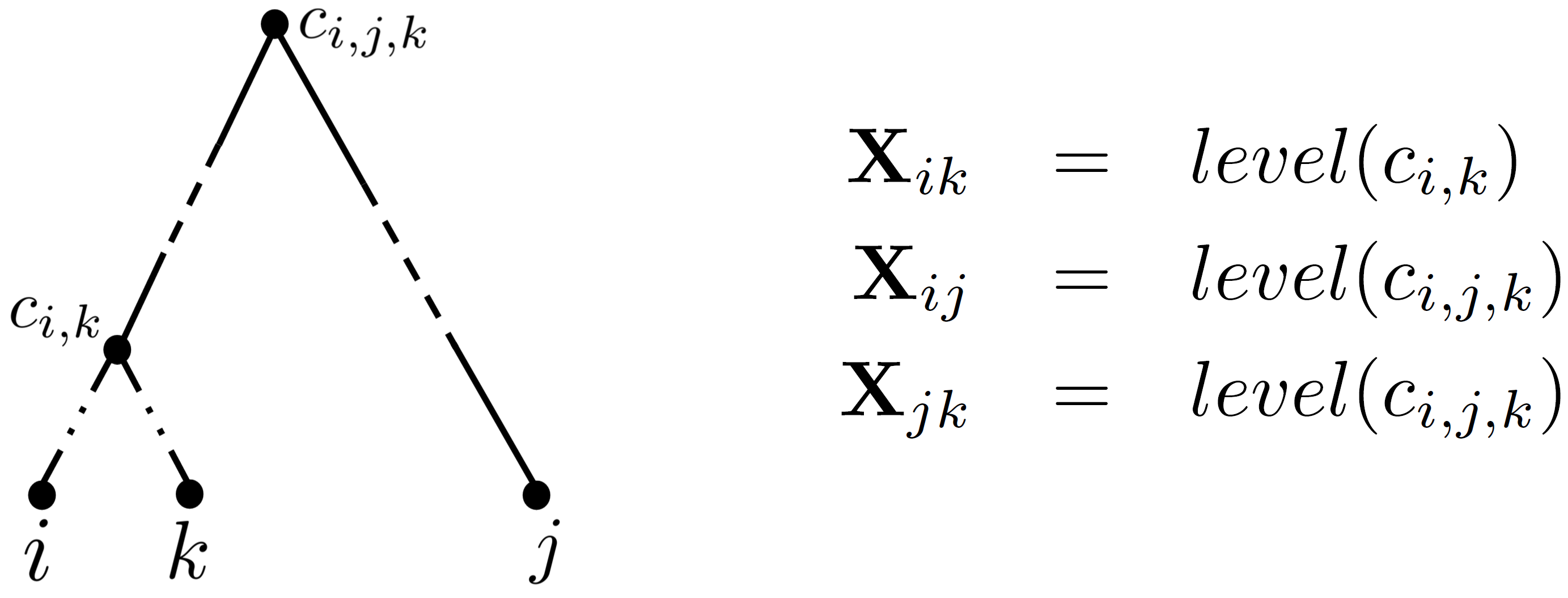
It is evident that when , the inequality in Eq. 9 is satisfied. Conversely, if , it implies that objects and are included in the same cluster (shown by ) before and join (to form cluster ). The bottom-up hierarchical clustering process then continues until is formed, encompassing all three objects . Notice that and join simultaneously via . In this case, according to Eqs. 8 and 9, and the relationships illustrated in Figure 1, we conclude
| (10) |
Ultrametric matrices, in turn, exhibit positive definiteness [28, 72], and such positive definite matrices result in inducing an Euclidean embedding [62]. Thereby, after ensuring the existence of such an embedding, we can employ a proper method to compute it. Specifically, we use the method proposed in [77] known as multidimensional scaling [55]. This method proposes first centering to obtain a Mercer kernel and then performing an eigenvalue decomposition. It works as follows.
-
1.
We center by
(11) where is an dimensional constant vector of ’s and is an identity matrix of size . With this centering, the sum of both the rows and columns in matrix becomes zero.
-
2.
With applying the transformation in step 1, becomes a positive semidefinite matrix, i.e., all the eigenvalues are nonnegative. Thus, we decompose into its eigenbasis:
(12) where represents the eigenvectors and is a diagonal matrix of eigenvalues .
-
3.
We calculate the matrix as the matrix of new data features:
(13) with and , where specifies the dimensionality of the new vectors.
In the embedded space, the new dimensions are arranged based on their corresponding eigenvalues. One can opt to select only the most significant ones, rather than utilizing all of them. Therefore, computing such an embedding also offers the benefit of feature selection. We also note that many clustering methods can be written in matrix factorization form via for example spectral -means [25]. This induces an embedding and hence a set of relevant features. However, for general positive/negative similarity matrices no exact embedding is feasible due to violating positive semidefiniteness. The method that we described here provides a solution to this challenge, i.e., enables us to extract features when the base pairwise similarities are positive and negative.
5 Correlation Clustering and Minimax Dissimilarities
Finally, we study minimax dissimilarities for correlation clustering, a graph-based method that corresponds to constructing a hierarchical clustering. Given graph , the minimax (MM) dissimilarity between and is defined as
| (14) |
where is the set of all paths between and over . Each path is specified by a sequence of object indices, i.e., indicates the object on the path.
Minimax dissimilarities enable a clustering algorithm to capture the underlying patterns and manifolds in an unsupervised and nonparametric way via extracting the transitive relations [42, 14]. For example, if object is similar to object , is similar to , and is similar to , then the minimax dissimilarity between and will be small, even though their direct dissimilarity might be large. The reason is that minimax dissimilarity finds the connectivity path and connects and via this path. This property is helpful in finding elongated clusters and manifolds of arbitrary shapes in an unsupervised way.
Minimax dissimilarities have been so far solely used with nonnegative pairwise dissimilarities. In the case of possible negative dissimilarities, we may use a trick similar to Proposition 1. As shown in Lemma 1, minimax paths are invariant w.r.t. the shift of the pairwise dissimilarities.
Lemma 1
Consider graphs and , where the pairwise dissimilarities (edge weights) in are shifted by constant , i.e., . Then, the minimax paths between every pair of objects and are identical on graphs and .
All the proofs are in Appendix A. Hence, given a dissimilarity matrix , one can subtract from all the elements to obtain . Then, the minimax dissimilarities can be computed from . After computing the minimax dissimilarities from , we may add to all the pairwise minimax dissimilarities. We can obtain the minimax similarities via , if needed.
We demonstrate that for correlation clustering there exists a simpler method to calculate the minimax dissimilarities intended for use in correlation clustering. According to Theorem 1, performing correlation clustering on minimax dissimilarities can be achieved in polynomial time via computing the connected components of the unweighted graph , where the similarity matrix is obtained by if , and otherwise.
Theorem 1
The optimal clusters of the correlation clustering on graph are equal to the connected components of graph .
As mentioned, correlation clustering on arbitrary similarity matrix is NP-hard [9, 23] and even is APX-hard [23]. Therefore, using minimax (dis)similarities with correlation clustering not only helps for extracting elongated complex patterns, but also yields a significant reduction in the computational complexity, i.e., from NP-hardness to a polynomial runtime.
Among the approximate algorithms proposed for correlation clustering on complete graphs with discrete weights, the method in [6] provides a 3-factor approximation. with a randomly selected unclustered object in the graph, this method greedily finds the object’s positive neighbors (those with similarity ) to form a new cluster. Then, it repeats this procedure for the remaining objects. One can conclude that in the optimal solution of correlation clustering on graph , exactly only the positive neighbors of an object will be in the same cluster as the object is, i.e., interestingly the 3-factor approximation algorithm in [6] becomes exact when applied to (Theorem 2).
Theorem 2
Assume the edge weights of graph are either or . Then, the approximate algorithm in [6] is exact when applied to the minimax similarities, i.e., to graph .
6 Experiments
In this section, we describe our experimental results on various datasets. We compare our methods with single linkage (SL), complete linkage (CL) and average linkage (AL).444 Some criteria, e.g. centroid, median and Ward compute a representative for each cluster and then compute the inter-cluster dissimilarities by the distances between the representatives. Computing such representatives might not be feasible for possibly negative pairwise dissimilarities. Thus, we do not consider them. As mentioned, there are several improvements over these basic methods. However, such contributions are orthogonal to our contribution. Moreover, it is unclear how such improvements can be extended to the dissimilarities that can be both positive and negative. Thus, we limit our baselines to these methods which as mentioned in Proposition 1, are applicable to such data.
In our studies, we have access to the true labels. Therefore, consistent with several previous studies on hierarchical clustering, e.g. [10, 5, 26], we evaluate the results according to the following criteria: i) Normalized Mutual Information (MI) [73] that measures the mutual information between the true and the estimated clustering solutions, and ii) Normalized Rand score (Rand) [37] that obtains the similarity between the two solutions. We do not use the labels to infer the clustering solution, they are only used for evaluation. Therefore, we are still in the unsupervised setting where the ground-truth labels play the role of an external evaluator.

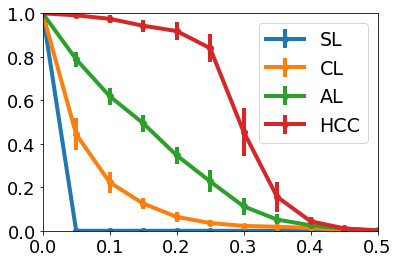
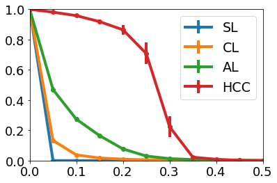
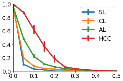
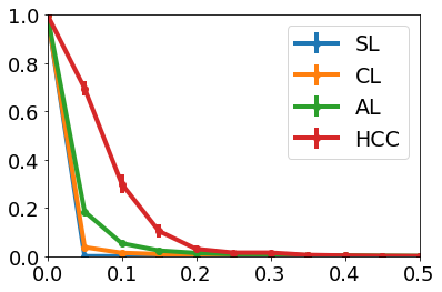
| Breast Tissue | Cardiotocography | Image Segm. | ISOLET | Leaf | One-Hun. Plant | |||||||
|---|---|---|---|---|---|---|---|---|---|---|---|---|
| method | MI | Rand | MI | Rand | MI | Rand | MI | Rand | MI | Rand | MI | Rand |
| SL | 0.006 | 0.008 | 0.007 | 0.007 | 0.008 | 0.001 | 0.009 | 0.016 | 0.008 | 0.003 | 0.015 | 0.020 |
| SL+GMM | 0.093 | 0.077 | 0.120 | 0.135 | 0.239 | 0.250 | 0.192 | 0.174 | 0.155 | 0.161 | 0.083 | 0.077 |
| CL | 0.227 | 0.166 | 0.077 | 0.056 | 0.187 | 0.125 | 0.057 | 0.017 | 0.081 | 0.038 | 0.029 | 0.008 |
| CL+GMM | 0.251 | 0.171 | 0.081 | 0.060 | 0.201 | 0.154 | 0.061 | 0.043 | 0.140 | 0.129 | 0.054 | 0.049 |
| AL | 0.542 | 0.519 | 0.391 | 0.479 | 0.518 | 0.495 | 0.257 | 0.165 | 0.181 | 0.106 | 0.066 | 0.023 |
| AL+GMM | 0.550 | 0.513 | 0.422 | 0. 463 | 0.522 | 0.501 | 0.240 | 0.179 | 0.152 | 0.143 | 0.081 | 0.065 |
| HCC | 0.903 | 0.900 | 0.987 | 0.994 | 0.945 | 0.943 | 0.938 | 0.918 | 0.429 | 0.373 | 0.159 | 0.104 |
| HCC+GMM | 0.914 | 0.911 | 0.979 | 0.974 | 0.960 | 0.966 | 0.941 | 0.917 | 0.462 | 0.401 | 0.183 | 0.217 |
6.1 HCC on UCI data
We first investigate the hierarchical correlation clustering on the following six UCI datasets chosen mainly from the image/shape domain [41].
-
1.
Breast Tissue: includes electrical impedance measurements of freshly excised tissue samples from the breast. The number of clusters is .
-
2.
Cardiotocography: contains measurements of fetal heart rate and uterine contraction features on cardiotocograms in clusters.
-
3.
Image Segmentation: contains samples from images of outdoor clusters.
-
4.
ISOLET: samples consisting of spoken attributes of different letters ( clusters).
-
5.
Leaf: images of leaf specimens originating from different plant species (clusters) each described by attributes.
-
6.
One-Hundred Plant: samples of leafs each described by features, from in total types (clusters).
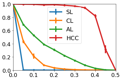
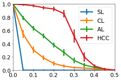
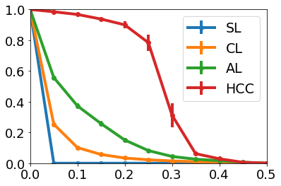
The ground-truth labels are shown by . We assume an oracle reveals the pairwise similarities according to the (flip) noise parameter . If then with probability and with probability . If then with probability and with probability . The function returns a uniform random number within the specified range. For each we repeat the experiments times and report the average results. This setup provides a systematic approach to study the robustness of various methods to noise.
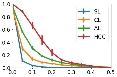
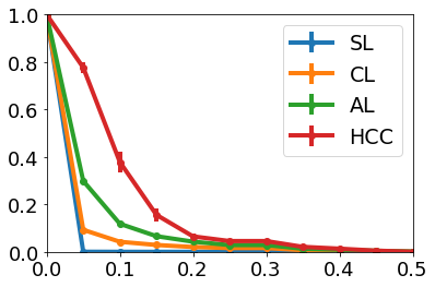
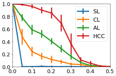
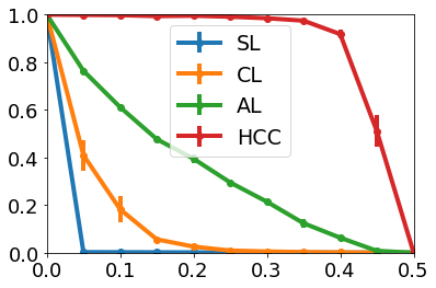
Figure 2 shows the results for different datasets as a function of the noise level w.r.t. MI. Rand scores shown in Figure 3 exhibits a consistent behavior. We observe that among different methods, HCC performs significantly better and produces more robust clustering w.r.t. the noise parameter . The results on Leaf and One-Hundred Plant are worse with all the methods. The reason is that these datasets are complex, having many clusters (respectively, and clusters) and fairly a small number of objects per cluster.
6.2 Tree preserving embedding of UCI data
In the following, we investigate tree preserving embedding and feature extraction. After computing the embeddings from different hierarchical clustering methods, we apply Gaussian Mixture Model (GMM) to the extracted features and evaluate the final clustering solution. This kind of embedding enables us to apply methods such as GMM to positive and negative similarities, a task that was not possible before. Since the extracted features appear in the form of vectors, thus, the final clustering method is not limited to GMM, and in principle, any numerical clustering is applicable.
Table 1 shows the results for different UCI datasets. We observe that the embeddings obtained by HCC (i.e., ‘HCC+GMM’) yield significantly better results compared to the embeddings from other methods (i.e., ‘SL+GMM’, ‘CL+GMM’ and ‘AL+GMM’). It’s worth noting that the results of embeddings (e.g., ‘HCC+GMM’) typically surpass the results obtained from the hierarchical clustering alone (e.g., ‘HCC’). This observation supports the idea that employing HCC to compute an embedding (for extracting new features) for a clustering method such as GMM may be advantageous, yielding superior results compared to using HCC exclusively for clustering purposes. This verifies why tree preserving embedding can be effective in general.
6.3 Experiments on Fashion-MNIST
Next, we investigate HCC and tree-preserving embedding on two randomly selected subsets of Fashion-MNIST dataset [75]. Fashion MNIST consists of images of Zalando’s articles. Each subset consists of samples/objects, where we compute the pairwise cosine similarities between them and then apply different methods. Table 2 shows the performance of different methods on these datasets. We observe that, consistent with the previous experiments, both ‘HCC’ and ‘HCC+GMM’ yield improving the results compared to the baselines. Furthermore, employing HCC to compute intermediate features for GMM (i.e., ‘HCC+GMM’) achieves higher scores compared to using ‘HCC’ alone for generating final clusters.
| Fashion MNIST 1 | Fashion MNIST 2 | |||
| method | MI | Rand | MI | Rand |
| SL | 0.322 | 0.206 | 0.241 | 0.196 |
| SL+GMM | 0.411 | 0.335 | 0.384 | 0.340 |
| CL | 0.403 | 0.293 | 0.546 | 0.379 |
| CL+GMM | 0.478 | 0.426 | 0.574 | 0.362 |
| AL | 0.464 | 0.468 | 0.602 | 0.534 |
| AL+GMM | 0.608 | 0.551 | 0.647 | 0.553 |
| HCC | 0.499 | 0.475 | 0.666 | 0.557 |
| HCC+GMM | 0.581 | 0.586 | 0.693 | 0.548 |
| news1 | news2 | news3 | news4 | |||||
|---|---|---|---|---|---|---|---|---|
| method | MI | Rand | MI | Rand | MI | Rand | MI | Rand |
| SL | 0.034 | 0.017 | 0.043 | 0.039 | 0.021 | 0.044 | 0.020 | 0.038 |
| CL | 0.266 | 0.277 | 0.255 | 0.230 | 0.501 | 0.594 | 0.121 | 0.116 |
| AL | 0.287 | 0.228 | 0.342 | 0.344 | 0.685 | 0.750 | 0.498 | 0.548 |
| HCC | 0.331 | 0.287 | 0.370 | 0.368 | 0.794 | 0.854 | 0.541 | 0.499 |
| news1 | news2 | news3 | news4 | |||||
|---|---|---|---|---|---|---|---|---|
| method | MI | Rand | MI | Rand | MI | Rand | MI | Rand |
| SL | 0.034 | 0.017 | 0.043 | 0.039 | 0.021 | 0.044 | 0.020 | 0.038 |
| SL+GMM | 0.191 | 0.158 | 0.108 | 0.097 | 0.166 | 0.210 | 0.134 | 0.120 |
| CL | 0.266 | 0.277 | 0.255 | 0.230 | 0.501 | 0.594 | 0.121 | 0.116 |
| CL+GMM | 0.271 | 0.275 | 0.272 | 0.239 | 0.522 | 0.587 | 0.118 | 0.119 |
| AL | 0.287 | 0.228 | 0.342 | 0.344 | 0.685 | 0.750 | 0.498 | 0.548 |
| AL+GMM | 0.309 | 0.279 | 0.358 | 0.350 | 0.701 | 0.773 | 0.503 | 0.525 |
| HCC | 0.331 | 0.287 | 0.370 | 0.368 | 0.794 | 0.854 | 0.541 | 0.499 |
| HCC+GMM | 0.344 | 0.297 | 0.439 | 0.443 | 0.831 | 0.892 | 0.560 | 0.519 |
| method | MI | Rand |
|---|---|---|
| SL | 0.218 | 0.192 |
| SL+GMM | 0.254 | 0.211 |
| CL | 0.386 | 0.417 |
| CL+GMM | 0.392 | 0.405 |
| AL | 0.459 | 0.488 |
| AL+GMM | 0.472 | 0.491 |
| HCC | 0.583 | 0.575 |
| HCC+GMM | 0.622 | 0.630 |
6.4 HCC on 20 newsgroup data
In the following, we study the performance of different methods on several subsets of 20 newsgroup data collection chosen randomly from different categories.
-
1.
news1: all the documents of the categories ’misc.forsale’, ’rec.motorcycles’, ’talk.politics.mideast’, ’sci.med’ ( dimensions).
-
2.
news2: all the documents of the categories ’alt.atheism’, ’comp.sys.mac.hardware’, ’sci.electronics’, ’soc.religion.christian’ ( dimensions).
-
3.
news3: all the documents of the categories ’sci.space’, ’soc.religion.christian’ ( dimensions).
-
4.
news4: all the documents of the categories ’comp.graphics’, ’rec.sport.baseball’, ’talk.politics.guns’ ( dimensions).
For each dataset, we compute the TF-IDF vectors of the documents and apply PCA with principal components.555The results are consistent with different number of components. We obtain the similarity between every two documents via the cosine similarity between their respective PCA vectors, which is a number in . We then investigate the different hierarchical clustering methods. Table 3 shows the results w.r.t. different evaluation criteria. Among the different methods, HCC usually yields the best results, and AL is the second best choice.
In the following, we investigate tree-preserving embedding on these datasets. Table 4 presents the results of tree-preserving embedding compared to hierarchical clustering. Specifically, we investigate the benefits of using hierarchical clustering for feature extraction. We observe, i) employing hierarchical clustering to extract features for a method such as GMM usually yields improving results, and ii) HCC, whether used directly for clustering or for feature extraction, often yields superior results compared to alternatives.
6.5 Experiments with web data
Finally, we investigate HCC for both hierarchical clustering and feature extraction on a web dataset. The dataset consists of webpages collected about topics such as politics, finance, sport, art, entertainment, health, technology, environment, cars and films. Similar to 20 newsgroup datasets, we compute the TF-IDF vectors, apply PCA and then obtain the pairwise cosine similarities between the web pages. Table 5 demonstrates the performance of different methods on this dataset. We observe that, consistent with the previous experiments, both HCC and HCC+GMM yield improving the results compared to the baselines. In addition, using HCC to compute intermediate features for GMM (i.e., HCC+GMM) provides slightly better scores than using HCC to produce the final clusters.
6.6 Correlation clustering with minimax dissimilarities
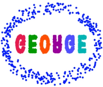
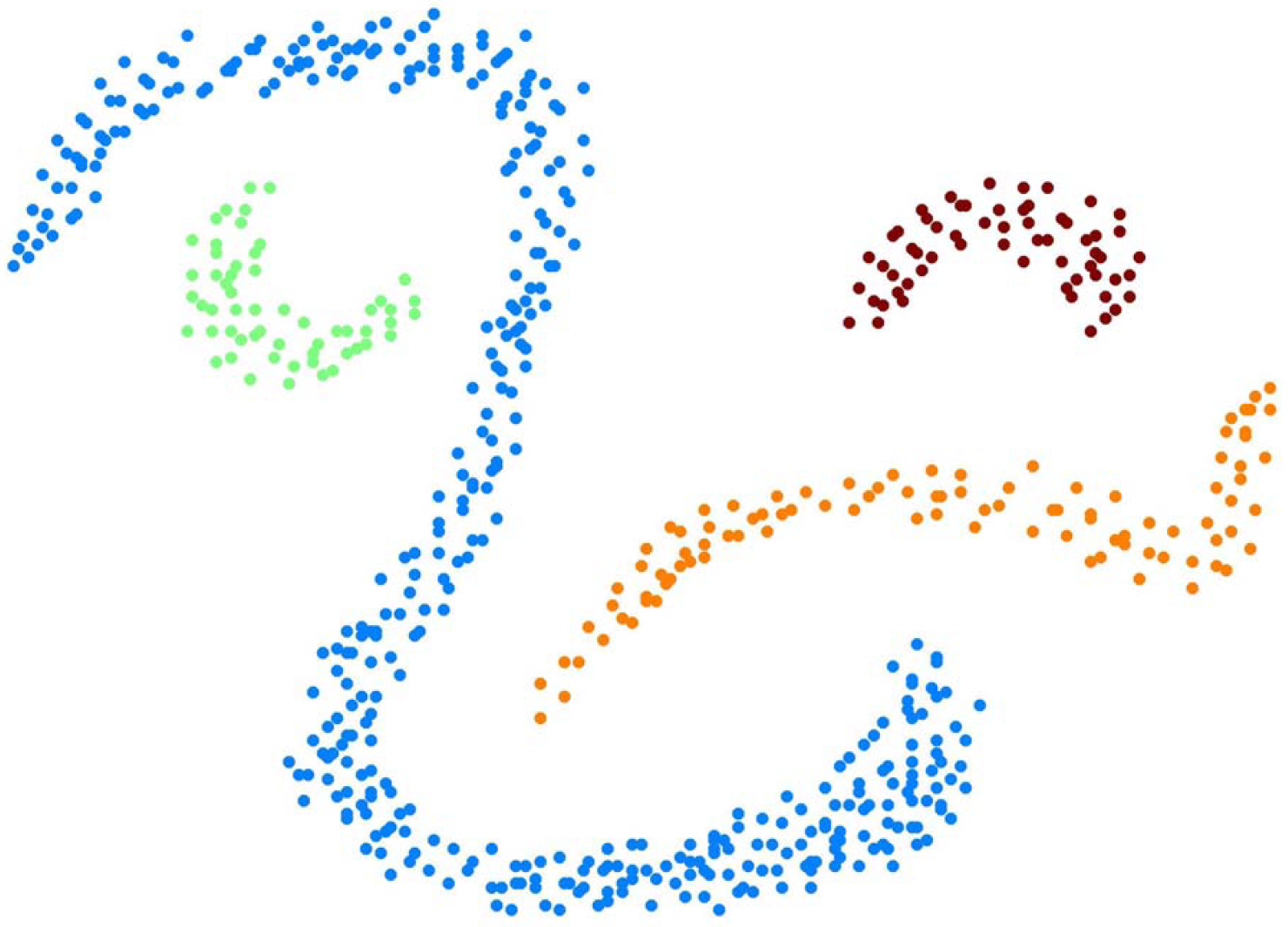
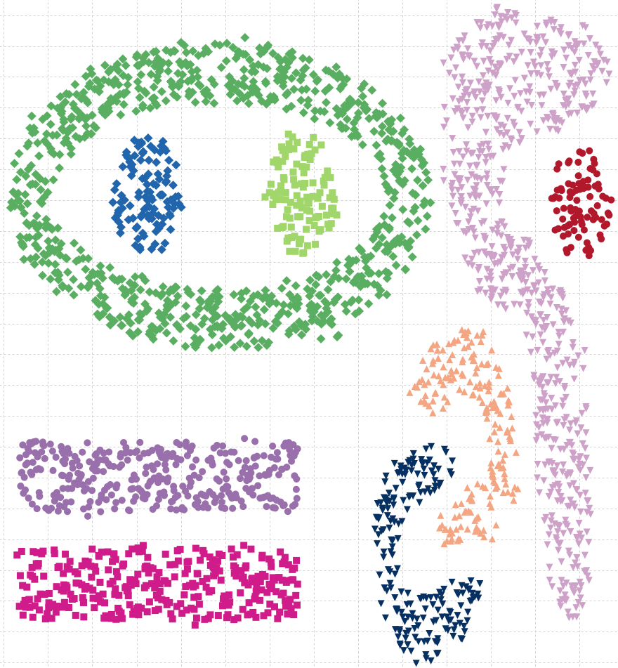
Finally, we investigate the use of minimax dissimilarities with correlation clustering. As mentioned, minimax dissimilarities are in particular useful for extracting elongated and complex patterns in an unsupervised way. Thereby, we apply ‘minimax + correlation clustering’ to a number of datasets with visually elongated and arbitrarily shaped clusters, and compare the results with ‘correlation clustering’ alone. The datasets are shown in Figure 4. For each dataset, we simply construct the K-nearest neighbor graph (using the ordinary Euclidean distance with a typical K such as 3). The edges in the nearest neighborhood receive a positive weight (e.g., +1) and a negative weight (e.g., -1) otherwise. We then apply either ‘minimax + correlation clustering’ or ‘correlation clustering’ to the resultant graph. We observe that for all the datasets, ‘minimax + correlation clustering’ yields the perfect clustering, i.e., MI and Rand are equal to 1. Whereas with ‘correlation clustering’ alone these scores are low, less than 0.2. We acknowledge the existence of other methods, such as DBSCAN [27], capable of achieving perfect clustering on these datasets. However, these methods often involve crucial hyperparameters, the tuning of which can be challenging in unsupervised learning. To our knowledge, in addition to computational and theoretical benefits, ‘minimax + correlation clustering’ stands out as the sole method capable of achieving perfect results on datasets with elongated clusters of arbitrary shapes, and fulfills the following two promises: i) it eliminates the need to fix hyperparameters, a task often intricate in unsupervised learning, and ii) it automatically determines the correct number of clusters without requiring prior fixing.
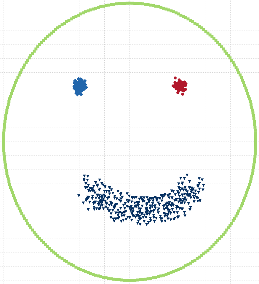
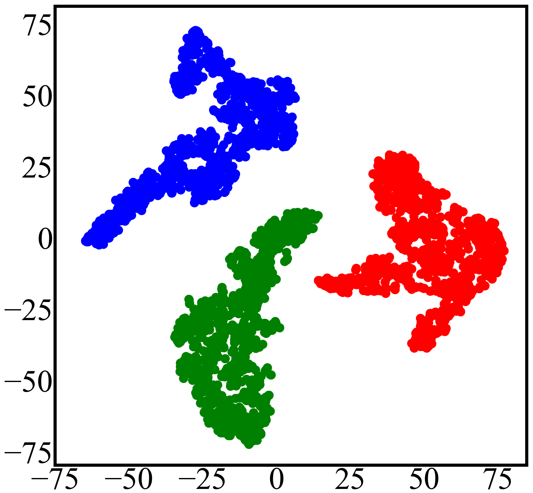
In the following, we consider the interesting application of clustering vehicle motion trajectories for ensuring safety in self-driving [35]. In this application, trajectories consisting of drive-by left, drive-by right and cut-in types are prepared, where some of them are collected in real-world and some others are generated using Recurrent Auto-Encoder GAN [24]. Next, dynamic time wrapping [11] and t-SNE [71] are employed to map the temporal data onto a two-dimensional space, as illustrated in Figure 5 [35, 24]. We then apply ‘minimax + correlation clustering’ to this data and compare it with ‘correlation clustering’. Similar to the datasets in Figure 4, ‘minimax + correlation clustering’ achieves perfect clustering with MI = Rand = 1 and accurately determines the correct number of clusters.
7 Conclusion
We proposed a new hierarchical clustering method, called HCC, suitable when the (dis)similarities can be positive or negative. This method is consistent with the general algorithmic procedure for agglomerative clustering and only differs in the way the inter-cluster dissimilarity function is defined. We then developed a framework for embedding the HCC dendrograms. Such an embedding provides extracting useful features to apply for example a GMM for clustering positive and negative similarities. In the following, we studied the use of minimax dissimilarities with correlation clustering and showed that it yields reduction in the computational complexity, in addition to a possibility for extracting elongated manifolds. Finally, we demonstrated the effectiveness of our methods on several datasets in different settings.
Acknowledgement
The work of Morteza Haghir Chehreghani was partially supported by the Wallenberg AI, Autonomous Systems and Software Program (WASP) funded by the Knut and Alice Wallenberg Foundation.
References
- [1] Clustering datasets. https://github.com/milaan9/Clustering-Datasets/.
- [2] Elke Achtert, Christian Böhm, Peer Kröger, and Arthur Zimek. Mining hierarchies of correlation clusters. In 18th International Conference on Scientific and Statistical Database Management, SSDBM, pages 119–128, 2006.
- [3] Margareta Ackerman and Shai Ben-David. A characterization of linkage-based hierarchical clustering. J. Mach. Learn. Res., 17:1–17, 2016.
- [4] Rakesh Agrawal, Alan Halverson, Krishnaram Kenthapadi, Nina Mishra, and Panayiotis Tsaparas. Generating labels from clicks. In International Conference on Web Search and Web Data Mining, WSDM, pages 172–181, 2009.
- [5] Julien Ah-Pine. An efficient and effective generic agglomerative hierarchical clustering approach. J. Mach. Learn. Res., 19:42:1–42:43, 2018.
- [6] Nir Ailon, Moses Charikar, and Alantha Newman. Aggregating inconsistent information: Ranking and clustering. J. ACM, 55(5):23:1–23:27, 2008.
- [7] Maria-Florina Balcan, Yingyu Liang, and Pramod Gupta. Robust hierarchical clustering. J. Mach. Learn. Res., 15(1):3831–3871, 2014.
- [8] Nikhil Bansal, Avrim Blum, and Shuchi Chawla. Correlation clustering. In 43rd Symposium on Foundations of Computer Science FOCS, 2002.
- [9] Nikhil Bansal, Avrim Blum, and Shuchi Chawla. Correlation clustering. Machine Learning, 56(1-3):89–113, 2004.
- [10] MohammadHossein Bateni, Soheil Behnezhad, Mahsa Derakhshan, MohammadTaghi Hajiaghayi, Raimondas Kiveris, Silvio Lattanzi, and Vahab S. Mirrokni. Affinity clustering: Hierarchical clustering at scale. In Advances in Neural Information Processing Systems (NIPS), pages 6864–6874, 2017.
- [11] R. Bellman and R. Kalaba. On adaptive control processes. Automatic Control, IRE Transactions on, 4(2):1–9, 1959.
- [12] Deepayan Chakrabarti, Ravi Kumar, and Kunal Punera. A graph-theoretic approach to webpage segmentation. In International Conference on World Wide Web, WWW, pages 377–386, 2008.
- [13] Moses Charikar, Venkatesan Guruswami, and Anthony Wirth. Clustering with qualitative information. In 44th Symposium on Foundations of Computer Science (FOCS), pages 524–533, 2003.
- [14] Morteza Haghir Chehreghani. Classification with minimax distance measures. In Proceedings of the Thirty-First AAAI Conference on Artificial Intelligence, pages 1784–1790, 2017.
- [15] Morteza Haghir Chehreghani. Clustering by shift. In IEEE International Conference on Data Mining (ICDM), pages 793–798, 2017.
- [16] Morteza Haghir Chehreghani, Hassan Abolhassani, and Mostafa Haghir Chehreghani. Improving density-based methods for hierarchical clustering of web pages. Data Knowl. Eng., 67(1):30–50, 2008.
- [17] Morteza Haghir Chehreghani, Alberto Giovanni Busetto, and Joachim M. Buhmann. Information theoretic model validation for spectral clustering. In International Conference on Artificial Intelligence and Statistics (AISTATS), 2012.
- [18] Morteza Haghir Chehreghani and Mostafa Haghir Chehreghani. Learning representations from dendrograms. Mach. Learn., 109(9-10):1779–1802, 2020.
- [19] Dongdong Cheng, Qingsheng Zhu, Jinlong Huang, Quanwang Wu, and Lijun Yang. A novel cluster validity index based on local cores. IEEE Trans. Neural Networks Learn. Syst., 30(4):985–999, 2019.
- [20] Michael Cochez and Hao Mou. Twister tries: Approximate hierarchical agglomerative clustering for average distance in linear time. In International Conference on Management of Data (ACM SIGMOD), pages 505–517, 2015.
- [21] Vincent Cohen-Addad, Varun Kanada, Frederik Mallmann-Trenn, and Claire Mathieu. Hierarchical clustering: Objective functions and algorithms. In SODA, pages 378–397, 2018.
- [22] Vincent Cohen-Addad, Varun Kanade, and Frederik Mallmann-Trenn. Hierarchical clustering beyond the worst-case. In Advances in Neural Information Processing Systems (NIPS), pages 6201–6209. 2017.
- [23] Erik D. Demaine, Dotan Emanuel, Amos Fiat, and Nicole Immorlica. Correlation clustering in general weighted graphs. Theor. Comput. Sci., 361(2-3):172–187, 2006.
- [24] Andreas Demetriou, Henrik Alfsvåg, Sadegh Rahrovani, and Morteza Haghir Chehreghani. A deep learning framework for generation and analysis of driving scenario trajectories. SN Comput. Sci., 4(3):251, 2023.
- [25] Inderjit S. Dhillon, Yuqiang Guan, and Brian Kulis. Kernel k-means: spectral clustering and normalized cuts. In Tenth ACM International Conference on Knowledge Discovery and Data Mining, SIGKDD, pages 551–556, 2004.
- [26] Laxman Dhulipala, David Eisenstat, Jakub Lacki, Vahab S. Mirrokni, and Jessica Shi. Hierarchical agglomerative graph clustering in nearly-linear time. In International Conference on Machine Learning (ICML), 2021.
- [27] Martin Ester, Hans-Peter Kriegel, Jörg Sander, and Xiaowei Xu. A density-based algorithm for discovering clusters in large spatial databases with noise. In Proceedings of the Second International Conference on Knowledge Discovery and Data Mining (KDD-96), pages 226–231, 1996.
- [28] Miroslav Fiedler. Ultrametric sets in euclidean point spaces. ELA. The Electronic Journal of Linear Algebra, 3:23–30, 1998.
- [29] Chris Fraley and Adrian E Raftery. Model-based clustering, discriminant analysis, and density estimation. Journal of the American Statistical Association, 97:611–631, 2002.
- [30] Lise Getoor and Ashwin Machanavajjhala. Entity resolution: Theory, practice & open challenges. Proc. VLDB Endow., 5(12), 2012.
- [31] C. Gower and G. J. S. Ross. Minimum spanning trees and single linkage cluster analysis. Journal of the Royal Statistical Society. Series C, 18(1), 1969.
- [32] Yi Gu and Chaoli Wang. A study of hierarchical correlation clustering for scientific volume data. In ISVC, pages 437–446, 2010.
- [33] Morteza Haghir Chehreghani. Shift of pairwise similarities for data clustering. Machine Learning, 2022.
- [34] Nicholas A. Heard. Iterative reclassification in agglomerative clustering. Journal of Computational and Graphical Statistics, 20(4):920–936, 2012.
- [35] Fazeleh Sadat Hoseini, Sadegh Rahrovani, and Morteza Haghir Chehreghani. Vehicle motion trajectories clustering via embedding transitive relations. In 24th IEEE International Intelligent Transportation Systems Conference, ITSC, pages 1314–1321. IEEE, 2021.
- [36] T.C. Hu. The maximum capacity route problem. Operations Research, 9:898–900, 1961.
- [37] L. Hubert and P. Arabie. Comparing partitions. Journal of classification, 2(1):193–218, 1985.
- [38] Bruce Hughes. Trees and ultrametric spaces: a categorical equivalence. Advances in Mathematics, 189(1):148–191, 2004.
- [39] Dmitri V. Kalashnikov, Zhaoqi Chen, Sharad Mehrotra, and Rabia Nuray-Turan. Web people search via connection analysis. IEEE Trans. Knowl. Data Eng., 20(11):1550–1565, 2008.
- [40] George Karypis. Cluto - a clustering toolkit, 2002. Retrieved from the University of Minnesota Digital Conservancy.
- [41] Markelle Kelly, Rachel Longjohn, and Kolby Nottingham. The UCI machine learning repository. http://archive.ics.uci.edu/datasets.
- [42] Kye-Hyeon Kim and Seungjin Choi. Neighbor search with global geometry: a minimax message passing algorithm. In Twenty-Fourth International Conference on Machine Learning, ICML, pages 401–408, 2007.
- [43] Sungwoong Kim, Sebastian Nowozin, Pushmeet Kohli, and Chang Dong Yoo. Higher-order correlation clustering for image segmentation. In Advances in Neural Information Processing Systems 24 (NIPS), pages 1530–1538, 2011.
- [44] Sungwoong Kim, Chang Dong Yoo, Sebastian Nowozin, and Pushmeet Kohli. Image segmentation using higher-order correlation clustering. IEEE Trans. Pattern Anal. Mach. Intell., 36(9):1761–1774, 2014.
- [45] Patrick K. Kimes, Yufeng Liu, David Neil Hayes, and James Stephen Marron. Statistical significance for hierarchical clustering. Biometrics, 73(3):811–821, 2017.
- [46] G. N. Lance and W. T. Williams. A general theory of classificatory sorting strategies. The Computer Journal, 9(4):373–380, 1967.
- [47] Bruno Leclerc. Description combinatoire des ultramétriques. Mathématiques et Sciences Humaines, 73:5–37, 1981.
- [48] Mark A. Levenstien, Yaning Yang, and Jurg Ott. Statistical significance for hierarchical clustering in genetic association and microarray expression studies. BMC Bioinformatics, 4(1), 2003.
- [49] Tom Liebmann, Gunther H. Weber, and Gerik Scheuermann. Hierarchical correlation clustering in multiple 2d scalar fields. Comput. Graph. Forum, 37(3):1–12, 2018.
- [50] Anna V. Little, Mauro Maggioni, and James M. Murphy. Path-based spectral clustering: Guarantees, robustness to outliers, and fast algorithms. J. Mach. Learn. Res., 21:6:1–6:66, 2020.
- [51] J. MacQueen. Some methods for classification and analysis of multivariate observations. In 5th Berkeley Symposium on Mathematical Statistics and Probability, pages 281–297, 1967.
- [52] Oded Maimon and Lior Rokach. Data Mining and Knowledge Discovery Handbook. 2005.
- [53] Álvaro Martínez-Pérez and Manuel A. Morón. Uniformly continuous maps between ends of $$\mathbbr$$ -trees. Mathematische Zeitschrift, 263(3):583–606, 2008.
- [54] Claire Mathieu and Warren Schudy. Correlation clustering with noisy input. In SODA ’10, pages 712–728, 2010.
- [55] A. Mead. Review of the development of multidimensional scaling methods. Journal of the Royal Statistical Society: Series D, 41(1):27–39, 1992.
- [56] Daniel Mullner. Modern hierarchical, agglomerative clustering algorithms. CoRR, abs/1109.2378, 2011.
- [57] Boaz Nadler and Meirav Galun. Fundamental limitations of spectral clustering. In Advances in Neural Information Processing Systems (NIPS), pages 1017–1024, 2007.
- [58] Andrew Y. Ng, Michael I. Jordan, and Yair Weiss. On spectral clustering: Analysis and an algorithm. In Advances in Neural Information Processing Systems (NIPS), pages 849–856, 2001.
- [59] Dehua Peng, Zhipeng Gui, Dehe Wang, Yuncheng Ma, Zichen Huang, Yu Zhou, and Huayi Wu. Clustering by measuring local direction centrality for data with heterogeneous density and weak connectivity. Nature Communications, 13(1), 2022.
- [60] J. Podani. Introduction to the exploration of multivariate biological data. Backhuys Publishers, 2000.
- [61] Aurko Roy and Sebastian Pokutta. Hierarchical clustering via spreading metrics. J. Mach. Learn. Res., 18(1):3077–3111, 2017.
- [62] I. J. Schoenberg. On certain metric spaces arising from euclidean spaces by a change of metric and their imbedding in hilbert space. Annals of Mathematics, 38(4):787–793, 1937.
- [63] Jessica Shi, Laxman Dhulipala, David Eisenstat, Jakub Lacki, and Vahab S. Mirrokni. Scalable community detection via parallel correlation clustering. Proc. VLDB Endow., 14(11):2305–2313, 2021.
- [64] Jianbo Shi and Jitendra Malik. Normalized cuts and image segmentation. IEEE Trans. Pattern Anal. Mach. Intell., 22(8):888–905, 2000.
- [65] A. Shieh, T. B. Hashimoto, and E. M. Airoldi. Tree preserving embedding. In International Conference on Machine Learning (ICML), pages 753–760, 2011.
- [66] A. D. Shieh, T. B. Hashimoto, and E. M. Airoldi. Tree preserving embedding. Proceedings of the National Academy of Sciences, 108(41):16916–16921, 2011.
- [67] Peter Henry Andrews Sneath. The application of computers to taxonomy. Journal of General Microbiology, 17:201–226, 1957.
- [68] R. R. Sokal and C. D. Michener. A statistical method for evaluating systematic relationships. Uni. of Kansas Science Bulletin, 38:1409–1438, 1958.
- [69] Jiliang Tang, Yi Chang, Charu C. Aggarwal, and Huan Liu. A survey of signed network mining in social media. ACM Comput. Surv., 49(3):42:1–42:37, 2016.
- [70] Erik Thiel, Morteza Haghir Chehreghani, and Devdatt P. Dubhashi. A non-convex optimization approach to correlation clustering. In The Thirty-Third AAAI Conference on Artificial Intelligence (AAAI), pages 5159–5166, 2019.
- [71] Laurens van der Maaten and Geoffrey Hinton. Visualizing data using t-sne. Journal of Machine Learning Research, 9(86):2579–2605, 2008.
- [72] Richard S. Varga and Reinhard Nabben. On symmetric ultrametric matrices. In Numerical Linear Algebra, 1993.
- [73] Nguyen Xuan Vinh, Julien Epps, and James Bailey. Information theoretic measures for clusterings comparison: Variants, properties, normalization and correction for chance. J. Mach. Learn. Res., 11:2837–2854, 2010.
- [74] Ulrike von Luxburg. A tutorial on spectral clustering. Statistics and Computing, 17(4):395–416, 2007.
- [75] Han Xiao, Kashif Rasul, and Roland Vollgraf. Fashion-mnist: a novel image dataset for benchmarking machine learning algorithms. CoRR, abs/1708.07747, 2017.
- [76] Pelin Yildirim and Derya Birant. K-linkage: A new agglomerative approach for hierarchical clustering. 17:77–88, 2017.
- [77] Gale Young and A. Householder. Discussion of a set of points in terms of their mutual distances. Psychometrika, 3(1):19–22, 1938.
Appendix A Proofs
A.1 Proof of Lemma 1
One can show that the pairwise minimax dissimilarities on any arbitrary graph are equivalent to the pairwise minimax dissimilarities on any minimum spanning tree derived from the same graph. The proof is similar to the maximum capacity problem [36]. Thereby, the minimax dissimilarities are obtained by
| (15) | |||||
where indicates the (only) path between and on the minimum spanning tree. To obtain the minimax dissimilarities , we select the maximal edge weight on the only path between and on the minimum spanning tree.
On the other hand, single linkage method and the Kruskal’s minimum spanning tree algorithm are equivalent [31]. Thus, the dendrogram obtained via single linkage sufficiently contains the pairwise minimax dissimilarities. Now, we need to show that the minimax dissimilarities in Eq. 15 equal the dissimilarities defined in Eq. 6, i.e., is the largest edge weight on the path between and in the hierarchy.
Given , let
| (16) |
Then, represents a minimum spanning subtree, which includes a path between and (because the root cluster of contains both and ) and it is consistent with a complete minimum spanning on all the objects. On the other hand, we know that for each pair of clusters which have direct or indirect parent-child relation, we have, iff . This implies the linkage of the root cluster of represents the maximal edge weight on the path between and represented by the dendrogram . Thus, represents
Thereby, minimax dissimilarities correspond to building a single linkage dendrogram and using the linkage as the pairwise dissimilarity between the objects in the two respective clusters. We know that according to Proposition 1 single linkage dendrogram is shift-invariant. Therefore, by shifting the pairwise dissimilarities by a sufficient , there will be no change in the paths between the clusters of single linkage dendrogram, nor in the paths representing the minimax dissimilarities.
A.2 Proof of Theorem 2
Over a graph, we define a path between and to be positive if all the edge weights on the path are positive. Then, we have the following observations.
-
1.
On a general graph , one can see that in the optimal solution of correlation clustering, if the two objects and are in the same cluster, then there is at least one positive path between them (the proof can be done by contradiction; if there is no such a path, then the two objects should be in separate clusters in order to avoid the increase in the cost function).
-
2.
Whenever there is a positive path between and , then their minimax similarity will be necessarily positive. Therefore, when we apply correlation clustering to graph , all the intra-cluster similarities of the optimal clusters will be positive. This corresponds to having a positive path between every two objects that are in the same optimal cluster, i.e., they are in the same connected component of where is defined as
(17) -
3.
We can also conclude that when we apply correlation clustering to graph , then for any optimal cluster , there is no object such that has a positive path to an object in . Otherwise, and all the other objects outside with positive paths to would have positive paths to all the objects in such that all of them should be clustered together.
Now we study the connection of connected components of graph to the optimal correlation clustering on .
-
•
There is a positive path between every two objects in a connected component of . Thus, they are in the same optimal cluster of .
-
•
If two nodes and are at two different connected components, then there is no positive path between them either on or on . Thus, they cannot be at the same cluster if we apply correlation clustering on .
Thus, we conclude that the connected components of correspond to the optimal correlation clustering on graph .
A.3 Proof of Theorem 3
The approximate algorithm in [6] iteratively picks an unclustered object and its positive neighbors as a new cluster. According to Theorem 1, the optimal solution of correlation clustering applied to corresponds to extracting the connected components of graph , where is defined in Eq. 17.
Thus it is sufficient to show the two followings.
- 1.
-
2.
If and are in different clusters according to algorithm [6] applied to , then . This indicates that there is no positive path between and on and also on , i.e., and are in different connected component of .
